Abstract
Mechanistic models are invaluable in ecological risk assessment (ERA) because they facilitate extrapolation of organism-level effects to population-level effects while accounting for species life history, ecology, and vulnerability. In this work, we developed a model framework to compare the potential effects of the fungicide chlorothalonil across four listed species of cyprinid fish and explore species-specific traits of importance at the population level. The model is an agent-based model based on the dynamic energy budget theory. Toxicokinetic-toxicodynamic sub-models were used for representing direct effects, whereas indirect effects were described by decreasing food availability. Exposure profiles were constructed based on hydroxychlorothalonil, given the relatively short half-life of parent chlorothalonil. Different exposure magnification factors were required to achieve a comparable population decrease across species. In particular, those species producing fewer eggs and with shorter lifespans appeared to be more vulnerable. Moreover, sequentially adding effect sub-models resulted in different outcomes depending on the interplay of life-history traits and density-dependent compensation effects. We conclude by stressing the importance of using models in ERA to account for species-specific characteristics and ecology, especially when dealing with listed species and in accordance with the necessity of reducing animal testing.
1. Introduction
In the United States, pesticide active ingredients are registered in accordance with the Federal Insecticide Fungicide and Rodenticide Act (FIFRA), as administered by the Environmental Protection Agency (USEPA), and must also be in compliance with the Endangered species Act (ESA), as administered by the Fish and Wildlife Service and National Oceanic and Atmospheric Administration Fisheries (collectively the “Services”). One of the requirements established by ESA is to ensure that any Federal action (i.e., registration of a pesticide active ingredient) does not jeopardize the existence of threatened and endangered (“listed”) species or contribute to the destruction of associated critical habitats [1,2]. Under FIFRA, the USEPA must ensure that registered pesticides do not cause unreasonable adverse effects on the environment, including listed species and their critical habitats. Although these federal statutes were stipulated decades ago, the establishment of a clear framework to address risks to listed species from the use of pesticides is a difficult task.
In this context, the National Research Council identified population modeling as a priority for listed-species ecological risk assessment (ERA; [3]). It is now established that population models are useful and relevant tools that can integrate potential effects of exposure to pesticides at the individual level with species-specific life-history traits, and to project effects to more relevant spatial and temporal scales [1,4]. Models are particularly valuable when assessing risks to listed species, especially at Step 3 where determinations are made on population viability and persistence. Models can extrapolate data generated from standard test species and consider those characteristics, such as life history, habitat use and requirements, or specific behaviors, that could influence the susceptibility of the exposed populations [1,5,6]. Even if species-specific data for model development is lacking, models can still provide insights on the relative importance of particular factors or processes that determine population persistence [1]. Finally, they can be used to explore the vulnerability of species of interest and help identify the most vulnerable representatives for each major taxonomic or functional group [6].
There have been growing efforts to improve model transparency, replicability, and guidance to facilitate and promote their use in ERA [4,7,8]. These include detailed guidance on model development, description, documentation, evaluation, and testing [9,10,11,12,13,14]. In particular, recent work has merged the decision guide [9] and the modeling framework [13] into a comprehensive approach for the development of population models for ERA. This approach, called Pop-GUIDE (Population modeling Guidance, Use, Interpretation, and Development for Ecological risk assessment), is applicable across regulatory statutes and assessment objectives and greatly facilitates the standardization of modeling development and use in ERA [8].
Here we developed a representative model for listed fish species following Pop-GUIDE. The primary goal was to explore species-specific traits and ecological processes of importance for determining the population dynamics of species exposed to a chemical. To this end, we used the available data at the individual level. The model has been developed to be flexible enough to address different risk-assessment questions. The model is agent-based (ABM), therefore, each individual is characterized by a set of state variables differentiating it from all other individuals. The model is based on Dynamic Energy Budget (DEB) theory, which describes the energy flow within an individual organism [15]. As a case study, we modeled the potential effects from exposure to the fungicide chlorothalonil on four cyprinid fish species, namely the Humpback chub (Gila cypha), Spikedace (Meda fulgida), Topeka shiner (Notropis topeka), and Devils River minnow (Dionda diaboli). These species were selected among a more comprehensive group of listed Cyprinidae for which DEB parameters are available (see the Add-my-pet database, www.bio.vu.nl/thb/deb/deblab/add_my_pet/) (accessed on 10 November 2020). Chlorothalonil was used as a case study given its ecotoxicological profile (e.g., it could adversely modify or destroy critical habitat, but not jeopardize listed species of interest, [16]). Because of the absence of monitoring data on chlorothalonil (which rapidly degradates in aquatic environments), exposure profiles were based on 4-hydroxy-2,5,6-trichloro-1,3-dicyanobenzene (also referred to as hydroxychlorothalonil or SDS-3701), a metabolite of chlorothalonil. We modeled both direct effects by implementing toxicokinetic-toxicodynamic (TKTD) models and indirect effects. We chose to use methods based on DEB theory and TKTD models because they are increasingly used in ecotoxicology and recognized for their relevance in representing ecotoxicity data [17,18,19].
2. Material and Methods
This section provides a summary model description following the overview and design concepts of the ODD (Overview, Design concepts and Details) protocol designed for describing ABMs (agent-based models) [10,20]. The model was developed following the guidance provided by Pop-GUIDE [8] (tables containing species-specific data in Supplementary Materials). A complete model description with a more detailed ODD is included in the TRACE (TRAnsparent and Comprehensive model Evaluation) documentation [21,22] in Supplementary Materials. The model was implemented in NetLogo 6.2 [23]; the model scripts, all relevant input files, including laboratory data used to calibrate effect submodels, as well as modeled exposure profiles are available on GitHub link https://github.com/Waterborne-env/DEB-based-Cyprinidae-Model (accessed on 10 November 2020).
2.1. Purpose
The purpose of the model is to represent and compare the population dynamics of multiple listed fish species exposed to time-variable concentrations under realistic habitat conditions. At the individual level, the metabolic processes are based on DEB (Dynamic Energy Budget) theory and are driven by temperature. Resource availability can also affect population dynamics when fish prey are exposed to the stressor. Each species is characterized by different DEB-parameter sets, mortality rates, density-dependent parameters, and environmental conditions (i.e., temperature and food drivers). Population dynamics emerge from interactions among individuals and between individuals and the environment and are affected by stochastic droughts. Chemical effects are based on laboratory data on the fungicide chlorothalonil and consider relevant effect endpoints, such as fish mortality, hatching success, egg production, and decreased food availability. Exposure profiles were predicated on the major metabolite 4-hydroxy-2,5,6-trichloro-1,3-dicyanobenzene (also referred to as hydroxychlorothalonil or SDS-3701) given the aerobic aquatic half-life of parent chlorothalonil ranges from 0.1 to 3.4 days, whereas hydroxychlorothalonil can persist in aquatic environments for several weeks [24]. Moreover, hydroxychlorothalonil is not relevant in terms of effects on aquatic organisms as parent chlorothalonil is orders of magnitude more toxic to fish and aquatic invertebrates. On an acute basis, chlorothalonil is classified as “very highly toxic” to fish and aquatic invertebrates (fish LC50 values range from 10.5 to 120 µg a.i./L and invertebrate LC50s are as low as 12 µg a.i./L), whereas hydroxychlorothalonil is classified as “slightly to moderately toxic (less toxic than parent) to aquatic organisms (96 hr LC50 = 9.2mg/L, Lepomis macrochirus; 48 h EC50 = 26 mg/L, Daphnia magna)” [24]. Consequently, whilst hydroxychlorothalonil was used as a worst-case surrogate for characterizing parent chlorothalonil exposures for the purpose of the case study, it is in no way predictive of potential environmental effects.
2.2. Species Modeled
The model represents the agents (individuals of four species of fish of the Cyprinidae family) and their environment. The selection was based on the following criteria: (i) data availability; (ii) goodness of DEB parametrization; (iii) ecological similarities; (iv) habitat similarities. We considered only riverine species that do not perform long migrations. The four species differ in habitat requirements and life-history traits such as size, lifespan, and fecundity. For example, the maximum length ranges from 41 cm (Humpback chub) to 5.5 cm (Topeka shiner). Humpback chubs usually live up to 5 years and produce more than 5000 eggs per year, whereas Devils River minnows have an average lifespan of 2 years and fecundity of 100 eggs per year (see the excel tables compiled following the Pop-GUIDE guidance in Supplementary Materials and the Addmypet website for more details). Humpback chub and Spikedace habitats partly overlap, the first species being endemic to the Colorado River Basin and the second to the Gila River system [25,26,27]. Topeka shiners live in pools of low-order prairie streams, oxbows, ponds, and dugouts in the Great Plains in the Midwest of the USA [28]. Finally, Devils River minnows occur in three tributaries to the Rio Grande: Devils River, San Felipe Creek, and Pinto Creek [29].
Cyprinidae are opportunistic feeders that switch diets depending on season and turbidity. Diet is mainly composed of microzooplankton, Chironomidae, Simuliidae, and amorphous detritus for chubs, daces, and shiners [30,31,32,33,34]. Minnows eat mostly filamentous green algae, blue-green algae, and diatoms [35].
Differences in environmental conditions for the four species are represented with different temperature profiles as well as differences in the seasonal availability of diet.
2.3. Process Overview and Scheduling
The conceptual model is summarized in Figure 1. The DEB equations describe the individual metabolic fluxes. DEB theory assumes that the assimilated energy goes into the reserve, which fuels metabolic processes and does not require maintenance. From the reserve, the energy is allocated to growth and structure maintenance or to maturity, maturity maintenance, and reproduction. Three life stages are represented: embryo, juvenile, and adult. Maturity energy thresholds define the switch among these stages. We use a variation of the standard DEB model: the abj model. The abj model is a general model used to represent the life cycle of fish, which takes into account the metabolic acceleration that occurs in early life stages [36]. This acceleration in growth is called “type M”, and takes place during a short period of time, starting at birth and ending before puberty (at a transition called “metamorphosis” in DEB theory). Individual state variables are updated based on a set of differential equations, and the model has been implemented as in [37,38]. The time step is equal to one day for all species but the Devils River minnow, for which we chose an hourly time step to have an energy increment across time small enough to represent the energy-threshold values correctly. Reproduction happens once a year, and the spawning day is chosen randomly within the species-specific reproduction period.
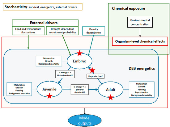
Figure 1.
Conceptual model diagram. The individual-level processes follow DEB rules and are represented in the blue box. External drivers such as drought-dependent mortality, food fluctuations, and chemical exposure are highlighted in green. The yellow box shows where stochasticity is introduced in the model. Density dependence affects embryo survival. The chemical affects organism-level processes including juvenile and adult survival, hatching success, and egg production (shown by the red stars).
Death after birth can occur because of background mortality, density dependence, drought, or chemical exposure. Background mortality is implemented stochastically using a uniform distribution. The stage-specific mortality rates have been adjusted to have the same lifespan as reported in the literature for each species. Density dependence results from cannibalism on eggs and larvae (embryos in DEB theory), a common feature among different species of Cyprinidae [39,40,41]. We implemented it as a Ricker function, assuming that embryo survival decreases with increasing adult biomass, as done by [33]. The modeled species are also particularly affected by habitat degradation and drought [26,42,43]. Drought frequency and extent are simulated based on data found in [44,45]. Drought-dependent mortality is represented by a stochastic reduction in recruitment following the empirical relationship given by [46].
Daily water temperature and daily food quantity are inputs to the model. We use three habitat-specific temperature profiles: Little Colorado River for chubs and daces, Devils River for minnows, and Midwestern habitat for shiners [33,47,48,49]. Similarly, we consider three different diet functions for the three habitats and represent the resource by a generic sine function with one or two peaks, depending on the habitat considered [50]. The assumed food function for chubs and daces has a peak around April-May and decreases in July, with a minimum value at the end of October. The food function for Devils River minnows has a minimum around January–February and a second minimum between July and August. The food function for Topeka shiners peaks in June and in December (see TRACE document in Supplementary Materials, Section 3.1). Food is abundant enough to be unlimited before adding indirect effects.
Finally, as stated previously, hydroxychlorothalonil, the major metabolite of chlorothalonil, was used as a highly conservative surrogate to generate exposure profiles due to the rapid degradation of parent chlorothalonil in aquatic environments.
2.4. Effect Implementation
Data from chlorothalonil toxicity studies conducted with fathead minnow (Pimephales promelas) were used to implement effects for the four modeled species (full life-cycle study: [51], reviewed by [52]; data analysis: [53]). Ref. [51] used nominal exposure concentrations of chlorothalonil between 0.6 and 16 µg/L. The test started with 200 fertilized eggs for each exposure concentration. It was split into distinct stages to accurately measure hatching success, post-hatching survival, total length and weight for the F0 and F1 generations, and reproductive success for the F0 generation. There were two replicate vessels for each test concentration, solvent control, and dilution-water control. The experiment showed effects on all endpoints except for fish growth. At the highest concentration, individual survival decreased up to 7%, and the number of eggs per female decreased by 98%. Furthermore, a slightly higher effect on post-hatching survival was found for the F1 generation with respect to the F0 generation for all tested chlorothalonil concentrations.
In our model, we simulate the effects of exposure to hydroxychlorothalonil (acting as a proxy for chlorothalonil exposure) by implementing four TKTD (toxicokinetic-toxicodynamic) models as toxic effects sub-models, representing four separate mechanisms of direct toxic action. The general unified threshold model of survival (GUTS), a simplified TKTD model of survival, was used to simulate lethal effects [54]:
- E1: toxicant-induced mortality of juveniles and adults (lethal effects, reduced GUTS-IT model);
- E2: decrease in egg production (sub-lethal effects, TKTD model);
- E3: decrease in hatching success (lethal effects, reduced GUTS-IT model);
- E4: decrease in food availability (indirect effects).
We used data on F0 post-hatching survival to parametrize the GUTS model reproducing juvenile and adult mortality, and data on embryo hatching success of the F1 generation to parametrize the GUTS model representing embryo mortality. This latter choice is more conservative because data showed a slightly higher effect in the F1 than in the F0 generation.
The reduced GUTS model expresses the internal damage (Di, [µg/L]) as a function of the external chemical concentration in the water (Cw [µg/L]) through the dominant rate constant kd [1/t]:
We ran both the IT (individual tolerance) and the SD (stochastic death) GUTS versions. In GUTS-IT, the individuals differ in their sensitivity to the chemical, whereas in GUTS-SD, toxicant-related mortality is a stochastic process. Since the GUTS-IT model best fitted the data, we used this version in our model and represented the threshold distribution describing the individual tolerance to the damage Di by the log-logistic Equation (2):
mw ([µg/L]) is the median of the threshold distribution, and β ([-]) is the shape parameter. We used the 2020 version of OpenGUTS in MATLAB to perform the calibrations (http://www.openguts.info/download.html, accessed on 20 April 2022). The survival probability is given by
where is the cumulative distribution of the thresholds calculated for the maximum scaled damage. In the ABM implementation, each individual is characterized by a defined threshold calculated using Equation (2), and when the external concentration exceeds the threshold, the individual dies.
Sub-lethal effects are represented by a DEB-TKTD sub-model describing the decrease in egg production. Because we only had data on egg production decrease and no evidence of effects on fish growth, we concluded that the adequate DEB physiological mode of action to represent these endpoints was a decrease in reproduction efficiency [-]:
The stress level s ([-]) is given by:
where c0 [µg/L] is the no-effect concentration, cT [µg/L] the tolerance gradient, that is the sensitivity to the toxicant at concentration levels above the NOEC, and Di, follows equation (1) with the same parameter value of as the GUTS model for juvenile and adult survival [55]. To set up the DEB-TKTD model, we assumed that c0 was equal to the reported NOEC (1.4 µg/L, [53]). Then, we calibrated the tolerance gradient cT on the data [51] through an optimization algorithm in R (optim).
Since the major food items of the fishes (i.e., aquatic invertebrates) can also be negatively impacted by chlorothalonil, we represented indirect effects as a decrease in food availability. We used a collection of LC50 and EC50 values calculated for 19 different aquatic invertebrate species exposed to chlorothalonil (Table 12 in the TRACE document) to build an SSD (Species Sensitivity Distribution). We considered this function a proxy for effect level [56], which is a conservative option as 100% effect is assumed based on LC50 and EC50 endpoint data. The distribution that best fitted the data was the Weibull function.
Parameter values for the four effect sub-models are listed in Tables 9–11 in the TRACE document. More information on the data and fitting can be found in the Supplementary Materials (TRACE documentation, Sections 2.7.9 and 3.3).
2.5. Exposure Scenarios
The population model was applied to evaluate chemographs of daily concentrations. Since daily monitoring data rarely exist for pesticides, available monitoring data from the National Water Quality Monitoring Council’s Water Quality Portal (WQP) were utilized by the SEAWAVE-QEX model [57] to generate the exposure profile necessary for population modeling. The WQP is the premier source of discrete water quality data in the United States, created by combining publicly accessible water quality data on a national scale, from the United States Environmental Protection Agency’s (USEPA) Storage and Retrieval Data Warehouse, the United States Geological Survey’s (USGS) National Water Information System, and over 400 state, federal, tribal, and local agencies [58]. SEAWAVE-QEX is a statistical model developed and released in 2018 by the USGS that simulates daily pesticide concentrations in surface water, from less-than-daily monitoring datasets, using streamflow and other covariates specific to a monitoring site [57].
To utilize monitoring data with SEAWAVE-QEX, the associated monitoring dataset must meet the following minimum data requirements described in Vecchia (2018):
- at least 3 individual years with 6 or more observations, 30 percent or more of which are uncensored;
- at least 30 observations for all years combined;
- at least 10 uncensored observations for all years combined.
All available monitoring data for chlorothalonil were downloaded from the WQP and queried for sites meeting these minimum data requirements. However, none of these sites met the minimum requirement of having at least 10 uncensored observations for all years combined. To account for the lack of chlorothalonil monitoring sites meeting the minimum data requirements for SEAWAVE-QEX, all available monitoring data for hydroxychlorothalonil were downloaded from the WQP and queried for suitable sites to be used as a surrogate. Of the resulting 854 monitoring sites in the WQP with monitoring data for hydroxychlorothalonil, 5 of the sites met all minimum data requirements. These 5 sites, all USGS monitoring stations, were in Georgia, Michigan, North Carolina, Oregon, and Texas, respectively (Figure S1 in Supplementary Materials—Exposure profiles). The USGS monitoring site in Texas, USGS-08057200, was ultimately selected for use with the SEAWAVE-QEX model, due to its relatively higher exposure values for hydroxychlorothalonil, which provided a more conservative exposure profile for population modeling.
SEAWAVE-QEX was run for years 2012–2020, using the model’s default input values (Table S2 in Supplementary Materials—Exposure profiles).
The daily mean concentration of the 100 conditional simulations was utilized to create a single exposure profile for population modeling (Figure 2). The hydroxychlorothalonil concentration values from this exposure profile ranged from 0.02 µg/L to 8.07 µg/L, with a mean concentration of 0.30 µg/L (Table S3 in Supplementary Materials—Exposure profiles).
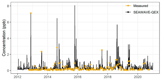
Figure 2.
SEAWAVE-QEX exposure profile for hydroxychlorothalonil at USGS-08057200.
2.6. Sensitivity Analysis
We performed a sensitivity analysis to check how changes in selected parameter values affected the total and the adult population abundances of Humpback chub and Topeka shiner. Performing the analysis on at least two species allows exploring if the simulated dynamics depend more on the model structure than on the represented species. We chose these two species because of the differences in their life-history traits. The sensitivity analysis was conducted by sampling the parameter space defined by ranges of 20 model parameters (out of 40 total model parameters): 12 core DEB parameters, background survival rates, density-dependence parameters, and the length of the reproductive periods. Reproduction starting and ending dates were changed to cover the more extensive time interval found in the literature (see PopGUIDE tables in Supplementary Materials). DEB parameters were modified by ±10% or ±2% (κ), whereas the other parameters were modified by ±25% (see Table 17 in the TRACE document). Following [59], the number of simulations (N) with a modified parameter set has to satisfy an empirical inequality: N > 4/3 * K, where K is the number of parameters. This ensures that the parameter space is sampled adequately. In our case, K = 20, therefore N has to be greater than 27. We sampled the parameter space 320 times using latin hypercube sampling [59] and repeated simulations with each parameter combination 20 times to account for model stochasticity, resulting in a total number of runs of 6400 performed for each species.
We did not perform a sensitivity analysis of the GUTS model because this had been done previously, and there is no need to report the influence of model parameters on model results on a case-by-case basis [18,60].
The results from the simulation runs were analyzed using a partial rank correlation (PRCC). This method was applied to assess the association between two random variables (here, the total or adult population abundance and one of the modified parameters) after the elimination of the effect of all other random variables (i.e., all the other modified parameters) [61].
2.7. Calibration, Simulation Experiments and Model Analysis
Species-specific DEB parameters have been previously estimated and are published in the Add-my-pet database (www.bio.vu.nl/thb/deb/deblab/add_my_pet/) (accessed on 10 November 2020). Because data on species-specific processes such as background mortality and density dependence were lacking, we adjusted relevant parameters (mortality rates, see TRACE document, Section 2.7.7) to achieve stable population dynamics and ensure that the lifespan of the organisms was as reported in the literature. We implemented density dependence as a Ricker function, assuming that survival of embryos decreased with increasing adult biomass as done in the model of [33]:
where B [g] is the adult biomass, and γ [1/g] is the steepness of the function (species-specific), and [1/t] is the background mortality of eggs. The food functions were calibrated based on the few available data concerning food item fluctuations (e.g., Chironomidae for chubs and daces, algae for minnows). A more comprehensive description of the data used to calibrate population dynamics and pesticide effects can be found in the TRACE document in Supplementary Materials (Sections 2.7 and 3).
We performed two kinds of simulations to evaluate the effects of pesticide exposure (Table 1). In the first case, all effect sub-models (E1, E2, E3, and E4) were applied simultaneously (i.e., they were all “switched on”). The hydroxychlorothalonil exposure profile was too low to reproduce the effects of chlorothalonil shown by Schults et al. [51]. Therefore, it was multiplied by different exposure magnification factors (EMFs)—ranging from 1 to 11—and used to evaluate the effects on the population dynamics of the four species. Secondly, we tested the relative importance of the different effect sub-models by sequentially adding the four mechanisms (“switching on” the different sub-models). We fixed the magnification factors for these simulations at 5 for Topeka shiner and Devils-River minnow, 7 for Spikedace, and 8 for Humpback chub. These different factors gave an overall decrease of species-specific population abundances by roughly 50% when all the effect sub-models were switched on. We started by simulating juvenile and adult mortality (first GUTS model, E1). We then progressively added the sub-lethal effects (TKTD model on egg production, E2), the reduction in hatching success (second GUTS model, E3), and indirect effects (decreased food availability, E4). Exposure lasted for five years and started a few years after population dynamics stabilized.

Table 1.
Simulation sets performed in the study. EMF = exposure magnification factor. E1 = GUTS model for juveniles and adults; E2 = TKTD model on egg production; E3 = GUTS model on hatching; E4 = indirect effects.
We represented the output as a relative decrease in population abundance during the five years of exposure for the first simulation set. To this end, we calculated the average ratio of the average population size under exposure over the average population size without exposure. We first calculated the mean population sizes over time (5 years), then we calculated the ratios exposed over non-exposed (40 ratios, equal to the number of replicates). Finally, we averaged the ratios over the 40 replicates. We also calculated the maximum and minimum value of the ratios to show its variability per scenario and species.
We performed the same analysis for the second simulation set by dividing the average exposed population by the average non-exposed population for the different effect sub-model contributions. We considered that the ratios of population abundances were significantly different from one scenario to the other (i.e., when adding up effects) if the relative differences of those ratios were greater than the arbitrarily chosen value of 5%:
where n is equal to the number of effect sub-models represented (1, 2, 3, or 4), and is the result when simulating one (or more) effect sub-model(s) and is the result when simulating two (or more) effect sub-models.
Finally, we looked at the average population abundances and biomasses of the total population and adults in the four scenarios and for each species.
3. Results
3.1. Baseline Population Dynamics
The four species’ population dynamics showed different oscillation patterns and did not stabilize in the same year (Figure 3). Total abundance values (# of individuals) of the stabilized population roughly vary between 180 and 1800 (Topeka shiner), 460 and 1150 (Devils River minnow), 200 and 1100 (Spikedace), 55 and 1500 (Humpback chub). The different stabilization times (roughly chosen five years after a clear stable dynamics) are year 15 for Topeka shiner and Spikedace, year 25 for Humpback chub, and year 20 for Devils River minnow. The dynamics of the four species are all characterized by yearly cycles, with high peaks corresponding to the after-spawning periods (birth of new individuals). Population dynamics of Humpback chub followed a different oscillation pattern from the other species, with 3–4 distinct yearly peaks.
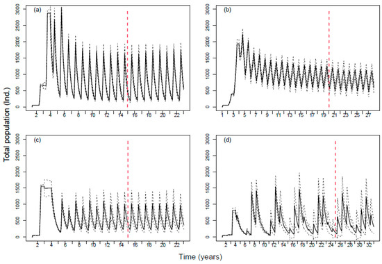
Figure 3.
Population dynamics for the four species (without chemical effects). Solid lines show the average population abundance over 40 replicates. Dotted black lines define the standard deviation. The red dotted line shows when we added the effects of the exposure (populations completely stabilized). (a) Topeka shiner; (b) Devils River minnow; (c) Spikedace; (d) Humpback chub.
3.2. Population Dose-Response
We applied the exposure profile shown in Figure 2 for five years (from 2012 to 2016) and simultaneously simulated all the effects. Exposure started in different years according to the species-specific stabilization periods. Figure 4 shows the ratio between the exposed and non-exposed populations during the 5-year exposure period. Topeka shiner and Devils River minnow had similar trends, characterized by a faster decline than the other two species for the same exposure magnification factors (EMF). The population abundances were about 50% of the control at EMF 5, and the species were extinct at EMF 7 and higher (see Figure S2 in Supplementary Materials—Population dynamics). Spikedace showed a less sharp decline: its total population abundance was about 50% of the control population at EMF 7. Finally, Humpback chub showed no effects up to EMF 5 (ratio close to 1). Exposed population abundance was 50% of the control population at EMF 8. Extinction of Spikedace and Humpback chub occurred at EMF 11. The variability decreased with increasing EMFs.
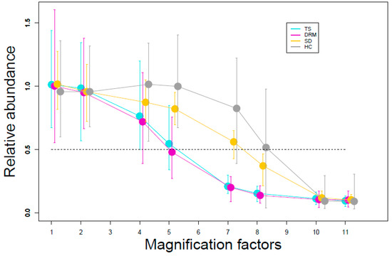
Figure 4.
Relative population abundance for different magnification factors of the exposure profile shown in Figure 2. Average populations are calculated over exposure time (5 years), the ratios of over-time averages are calculated for each replicate, and then ratios are averaged over 40 replicates. The bars show the maximum and minimum value of the ratio among the 40 replicates. Symbols and bars are shifted for visual reason. TS: Topeka shiner; DRM: Devils River minnow; SD: Spikedace; HC: Humpback chub.
3.3. Effect sub-Models
When simulating the first effect sub-model alone (using the species-specific EMFs defined above), Humpback chub and Spikedace population abundances were less affected than the other two species (Figure 5). However, there was a significant effect on population biomass for all four species (Figure 6), reflecting a change in population size distribution. Adding the effect sub-model E2 affected especially the Spikedace population, for which both abundance and biomass decreased, and to a lesser extent, the Humpback chub population. No significant changes (i.e., changes greater than 5% in population abundances) were seen for the other two species. Adding E3 affected all four species’ population abundance and biomass, whereby Humpback chub showed the highest effect size. Finally, adding E4 affected only the dynamics of Humpback chub, which showed a slight increase in both abundance and biomass. In summary, relative differences between consecutive ratios were smaller than 5% (and therefore considered not significant) when adding the effect on egg production for Topeka shiner and Devils River minnow, and when adding indirect effects for all species but the Humpback chub (Table S2 and S3 in Supplementary Materials—Population dynamics). The Humpback chub population had the highest variability in the 4 cases.
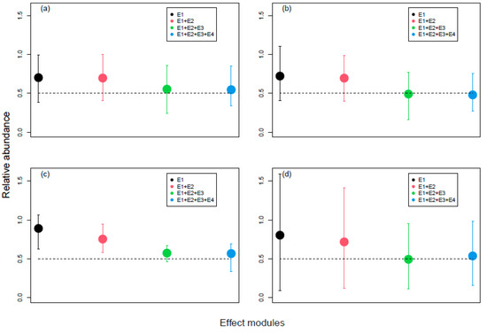
Figure 5.
Relative population abundances of the four species in the second simulation set, i.e., where effect sub-models were sequentially added. Average populations are calculated over the exposure time (5 years), the ratios of over-time averages are calculated for each replicate, and then ratios are averaged over 40 replicates. The bars show the maximum and minimum value of the ratio among the 40 replicates. (a) Topeka shiner (EMF = 5); (b) Devils River minnow (EMF = 5); (c) Spikedace (EMF = 7); (d) Humpback chub (EMF = 8).
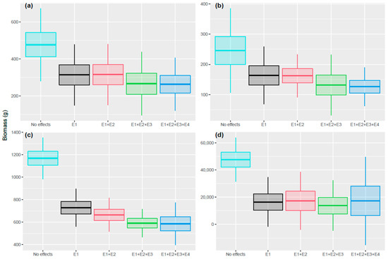
Figure 6.
Average population biomasses for control simulations and when sequentially adding effect sub-models. Averages are calculated over exposure time (5 years) and over 40 replicates. The middle lines represent the mean biomass values, the boxes define the standard deviation, and the bars show three times the standard deviation. Different colors represent the tested effect scenarios. (a) Topeka shiner (EMF = 5); (b) Devils River minnow (EMF = 5); (c) Spikedace (EMF = 7); (d) Humpback chub (EMF = 8).
3.4. Sensitivity Analysis
The sensitivity analysis showed that the most influential parameter for the four outputs (i.e., total and adult abundance of Humpback chub and Topeka shiner) was κ, the DEB parameter determining the energy allocation to growth/maintenance and to maturation/reproduction. Other sensitive parameters were those defining background mortality rates and density dependence. Total and adult population abundances were affected almost equally by parameter changes. The only remarkable difference was noticed in juvenile and adult mortality rates in the case of Humpback chub: the total population was less affected by changes in those parameters than the adult abundance, probably because of density-dependence compensation mechanisms. Furthermore, there were a few differences between the two species: Topeka shiner abundance was more sensitive to changes in the energy-threshold parameters. Finally, some parameter combinations caused the populations to go extinct (see TRACE document, Section 7).
4. Discussion
We developed an agent-based model, following the decision steps from Pop-GUIDE [8], to compare population-level responses of four listed Cyprinidae species exposed to the fungicide chlorothalonil as a case study. The model combines lethal and sublethal effects on individual fish and accounts for density dependence and drought stochasticity. Chlorothalonil was selected as a case study based on its ecotoxicological profile (i.e., direct effects via toxicity to fish and indirect effects via toxicity to aquatic invertebrates and plants [24]). Hydroxychlorothalonil, the major environmental metabolite of parent chlorthalonil, was used as a worst-case proxy for exposure as chlorothalonil degrades rapidly in aquatic environments. We found that the simulated Devils River minnow and Topeka shiner populations were the most vulnerable of the four modeled species. Applying different effect submodels separately revealed that reducing adult and juvenile survival and hatching success had the biggest impact on populations of the four modeled species. Population biomass abruptly declined when reducing adult and juvenile survival, especially in the Humpback chub population. These results highlight the importance of considering life-history traits and density dependence when assessing exposure consequences at the population level. In this section, we analyze further the model outputs and discuss different aspects linked to data quality and quantity, often present when dealing with listed species and the adaptation of lab results to model inputs.
4.1. Baseline Population Dynamics
The baseline population dynamics of the four simulated species showed both similarities and differences. Because reproduction happens once a year in a specific period, all the species had yearly abundance fluctuations. However, the amplitude and pattern of these oscillations were species-specific and resulted from the interplay among life-history traits, background mortality rates, and density dependence. The four species differ in their lifespan, size, and reproductive output. For example, Humpback chub lifespan is about 5 years [62] (although some specimens can reach an age of 30 years, [63]), whereas Spikedace can live up to 4 years [27], Topeka shiner live up to 3 years [64], and Devils River minnow live up to 2 years [29]. Moreover, Humpback chub has a total length almost eight times the length of Topeka shiner, seven times of Devils River minnow, and more than four times of Spikedace [65,66,67,68]. Because fecundity is usually size-dependent for fish species, Humpback chub produces more eggs per year than the other species (about 5000 eggs per year, while Spikedace produces roughly 1200 eggs per year, Topeka shiner 830 eggs per year, and Devils River minnow 100 eggs per year) [35,66,69]. One way in which these traits could affect the population dynamics is through intraspecific competition. Competition is often driven by size, and it is one major factor determining population size structure, especially in fish [70]. However, in our model, organisms do not compete for food without exposure because we did not find evidence in the literature of density-dependent food limitation. Therefore, we looked at the role played by another form of density dependence, since fish populations can also be affected by size-dependent cannibalistic interactions between different age cohorts [70,71]. Because we aimed to achieve stable population dynamics, density dependence was calibrated differently for each species, as it strongly depended on total adult biomass and, consequently, on the size of different modeled species. We found that density dependence significantly affected the simulated dynamics of Humpback chub (Figure S2 in Supplementary Materials—Population dynamics), most likely due to the largest individual size and overall population biomass. Stochastic drought events did not significantly impact the simulated dynamics, except for a negligible effect on Devils River minnows (Figure S1 in Supplementary Materials—Population dynamics). Droughts are simulated as an additional mortality factor, which occurs only a few times in the simulated time span, and the reduction in recruitment is uncertain. Despite habitat degradation and drought being among the major causes of population decline for these species [26,42,43], data on the effects of drought are rare. For Cyprinid fish in North America, we could find only a single study on Roundtail chubs, which identified a link between water scarcity and reduced recruitment ([46]; see TRACE document for more details, Section 3.2). A detailed evaluation of the effects associated with drought (and other natural stressors) on the represented species would greatly improve model adequacy, allowing a more realistic and comprehensive risk assessment under chemical exposure.
4.2. Population-Level Responses to Exposure
The exposure profile applied for the current case study corresponds to the highest concentrations of hydroxychlorothalonil observed in available monitoring data in rivers across the US. This metabolite of chlorothalonil was used as a proxy for realistic exposures in streams because the detected chlorothalonil concentrations were not sufficient for the estimation of realistic exposure profiles. Consequently, none of the monitoring sites for chlorothalonil acquired from the WQP met the minimum requirement for SEAWAVE-QEX.
Evaluation of the worst-case exposure profile (corresponding to the USGS monitoring station in Texas for hydroxychlorothalonil) with the population model did not result in any modeled effects on simulated populations. Exposure magnification factors (EMFs) were applied to compare the responses of the simulated species. Population-level responses to hydroxychlorothalonil exposure varied across the four species, with Topeka shiner and Devils River minnow populations being more affected at a lower EMF (≥3) than the other two species. This difference can be explained by species-specific life-history traits. Notably, Topeka shiner and Devils River minnow have smaller sizes and shorter lifespans than Humpback chub and Spikedace, which means fewer eggs and fewer total spawning events in their lives, respectively. Consequently, simulated populations of Topeka shiner and Devils River minnow were more vulnerable, and complete recovery after high exposure levels was less likely than in the case of Spikedace and Humpback chub (see Figure S3 in SI-Population dynamics). Other studies have highlighted the importance of considering life-history traits to understand species-specific responses to exposure [72], and fecundity has also been shown to influence population responses after exposure [37,73]. Therefore, trait-based approaches can be particularly useful in addressing listed species ERA, for which data are often unavailable or difficult to collect [5]. Characterizing and understanding the effects of a given stressor on species with similar traits facilitates inference of corresponding effects on listed species by further allowing extrapolation across levels of organization or exposure regimes [74]. However, to protect such rare taxa, it is imperative that appropriate and vulnerable traits are included in the analysis and modeling [74]. Traits like taxonomic group, lifespan, maximum size, number of generations per year, fertility, and mortality rates are among those considered to influence vulnerability [6,75,76,77]. Consistent with these previous studies, our results suggest that these same types of traits are responsible for the observed species-specific differences in responses to stressors. However, such data are often unavailable for listed species, which is a major challenge for trait-based approaches in ERA [74,78] and specifically for listed species risk assessments. Finally, other species- and/or system-specific factors play a role in differential species population vulnerability. For example, in our case, the higher vulnerability of the two smaller species (Topeka shiner and Devils River minnow) could partly also result from the weaker density dependence and consequent lower compensation responses under exposure. By integrating species-specific life-history information with other relevant processes, we could identify the most vulnerable populations among the four simulated species. Future applications of population models should increasingly include quantitative vulnerability analyses which could lead to more streamlined risk assessments as well as targeted data collection, when possible.
4.3. Assessment of Effect Sub-Models
It is crucial to consider the potential of the multiple effects of a stressor to fully capture exposure consequences at the population level [79]. Sequentially adding the effects of various effect pathways may result in unpredictable interactions depending on the species and the level of biological organization considered [80,81]. Here we tested if sequentially adding effect sub-models could affect the fish populations differently depending on species-specific characteristics and parameter calibration. To this end, we added one sub-model at a time and compared population-level responses across species. When all effect sub-models were applied in parallel, the population abundance decreased progressively for all species. Still, there are some notable species-specific differences in the responses. When only E1 was applied (i.e., the GUTS model for juveniles and adults), Topeka shiner and Devils River minnow populations showed a sharp decline in abundance. In contrast, Spikedace and Humpback chub populations showed a slight decrease in size and a marked change in size distribution. In the latter case, the highest mortality of juveniles and adults decreased the density-dependent pressure on embryos, allowing for higher recruitment but lower total population biomass (Figure 6). In addition to life-history traits such as overall reproductive effort, which are known to drive recovery after exposure [82], the species-specific density-dependent compensation dynamics may have played an important role in the different population-level responses. Previous work has explored the role of density dependence in toxicant-exposed populations [83,84,85,86]. Density dependence may interact with stressor effects in complex ways (e.g., synergistic or antagonistic) depending on the type of density dependence and the resulting level of compensation [84,85]. Often the interaction between stressor and density is not linear [87], and compensation can occur for some forms of density dependence (e.g., on survival) and not for others (e.g., on growth) [85]. In our model, we used the same function across the four species, but the parameterization differed to produce stable dynamics, which might have resulted in additional differences in across-species responses.
Adding E2 (sublethal effects on egg production) affected only the Spikedace population and mildly the Humpback chub population. The difference among species depends on the different EMFs we used (higher for Humpback chub and Spikedace) and the exposure profile. Because there was almost no overlap between the highest exposure peaks and the reproductive periods, a high EMF was needed to observe effects on egg production. In the case of Humpback chub, this extra effect sub-model is probably still compensated by density dependence (fewer individuals means less cannibalism in the following generations). Our findings suggest that egg production decline does not have a large effect on population dynamics, a result already highlighted by previous work (e.g., [88]). Furthermore, analysis of life-history trait elasticity has shown that fecundity (or fertility) generally has low elasticity, meaning that changes in it have a small impact on population growth rate [89,90]—a finding also assigned to release from competition for resources.
Including E3 (decrease in hatching success) resulted in a decrease in both population abundance and biomass, especially in the Humpback chub. This additional GUTS model has very fast kinetics and causes higher mortality for those species exposed to higher EMFs. Moreover, the longer the embryo phase, the higher the internal chemical concentration in the organisms. Since Topeka shiner and Devils River minnow have a relatively shorter embryo period and are at lower EMF, the relative difference in effect size with respect to the previous scenario (i.e., E1 + E2) is smaller than for Humpback chub. Nevertheless, Devils River minnow is more affected than Topeka shiner and Spikedace. Devils River minnow has the lowest egg production of the four species, and adding extra mortality has a more considerable impact on its population despite the lower EMF.
Finally, including indirect effects did not cause any significant change to the population dynamics. Only the Humpback chub showed a slight increase in both abundance and biomass. However, the relative difference compared to the previous scenario (E1 + E2 + E3) was small (8% for population abundance), and the variability high. A possible explanation for the change in the average population abundance could be that decreasing food affects fish size and egg production, allowing for density-dependent compensation. Different dynamics can arise depending on the population size and structure when food is depleted, explaining the high variability. In some cases, the interplay between mortality rates, density dependence, and population fluctuations can lead to increased population sizes with increased mortality rates (hydra effect) [86,91].
4.4. Model and Data Limitations
Our work shows that life-history traits and population-level processes are essential to forecast exposure effects on the population dynamics of listed species. These results are built on, and supported by, other studies in the literature. However, as models represent simplifications of real systems, our work presents some limitations linked to model structure, data availability, and data quality. Recognizing methodological limitations (of both in vivo and in silico experiments) is fundamental to understanding study uncertainties and guiding future developments. The first limitation derives from the DEB parametrizations, which are data demanding and therefore affected by a lack of data for listed species. Among the required data sets to obtain a proper calibration of fish species (abj model), there are threshold ages, lengths, and weights (e.g., age at birth or length at metamorphosis) [92,93]. Unfortunately, none of the modeled species had information on metamorphosis. Therefore, the estimation of the metamorphosis energy threshold is highly uncertain [93]. Moreover, we found gaps in those datasets that allow calibrating the other maturity thresholds (energy at birth and puberty). Failing to correctly predict these values, which are key events in the life cycle and vary considerably among species, could lead to a mis-estimation of the time spent in a particular life stage and potentially affect modeling results when considering life-stage dependent effects of stressors [93]. However, even if some data points (called zero-variate) were missing for the four species, it is worth noticing that additional data functions (called uni-variate) were present, which greatly improved parameter estimation and increased confidence in the DEB calibration [94]. We encountered some problems with model implementation mainly when dealing with Devils River minnow. To represent this fish species, we had to change the time step from daily to hourly to capture the tiny increase between energy at birth and energy at metamorphosis (which differs by only 0.008 J). Furthermore, we had issues calculating length and energy density increments, probably because of a poorer DEB parametrization (higher mean relative error, or MRE, than the other species).
The sensitivity analysis also highlighted the importance of having good data quality and gave insights on how future sampling efforts could be more informative for modeling purposes. For example, modeled outputs were highly sensitive to minor variations of the value of κ, a central parameter in DEB theory. κ defines which fraction of the assimilated energy goes from the reserve to maturation/reproduction and growth/maintenance. While no defined data set affects the accuracy of κ calibration, the more data that are available on the organism’s life cycle, the better is the calibration. Another result of the sensitivity analysis stressed the importance of having a good parameterization of the energy threshold levels. The population abundance of Topeka shiner was particularly sensitive to changes in these parameters. Interestingly, this was not the case for the Humpback chub. The reason probably lies in the fact that there is a small difference between threshold values in the case of Topeka shiner. If, for instance, the modified value of maturity energy at birth is too close to the maturity energy at metamorphosis, maturity switches could happen at the wrong sizes, and the entire life cycle could be compromised. Finally, another important and expected result of the analysis was that population abundances were highly sensitive to changes in the background survival rates. Therefore, field studies that collect data on species lifespans, size or age distributions, and average stage-specific survival rates could improve model performance.
The second limitation of our model is the quality of the pesticide effects data. We based our representation of pesticide effects on the laboratory study by [51]. This study looked at the chronic toxicity of chlorothalonil on fathead minnow during two generations (see the TRACE document for a complete description of the data, Section 3.3). There are a few notable limitations with the study. First, there were only two replicates for the two control tests (solvent and dilution water) and the exposure tests. This is potentially problematic because all fish accidentally died between 16 and 33 days in one replicate of the controls. Secondly, the study was started with 200 eggs. During the study conduction, the authors randomly selected a subset of individuals on day 64 and then again on day 172 to continue the experiment. Therefore, the number of tested organisms was relatively small, and it was impossible to recalculate the correct background mortality throughout the test because of the selection process. To verify if the GUTS model could reproduce juvenile and adult mortality data, we adapted our model for the fathead minnow (parameters from [86]). The model could not match the data perfectly up to concentrations of 3 µg/L but reproduced the higher mortality rates at 6.5 and 16 µg/L, which were the only ones showing a clear trend in the data (see Tables 13 and 14 on the TRACE document). It is unclear what caused the high mortality at 3 µg/L in the experiment. If it was caused by unexpected high background mortality (as suggested by the lab reports), then exposure was not the cause, in accordance with the low mortality observed for 6.5 µg/L. The calibration of the second GUTS model for hatching success was more challenging because of the presence of only two data points: (introduction of the eggs into the experiment) and days (time at hatching). GUTS models need to have multiple data points to perform a good calibration (at least 5, [18]). Consequently, we had different parameter values each time we ran the calibration algorithm. Despite these problems, we could correct for background mortality in this case, and we obtained a parameter set that allowed us to match the data.
Finally, the parametrization of the TKTD representing the decrease in egg production was not straightforward because we could not directly retrieve the stress values from the theoretical linear Equation (4). However, the values we obtained through the optimization process reproduced the data reasonably well (Table 16 in the TRACE document).
In conclusion, despite the numerous data gaps, we could calibrate all the sub-models and represent the empirical data well. It is important to emphasize that due to animal welfare concerns, it is unlikely that ecotoxicological studies will be repeated unless there are safety concerns. This is even more so true for the case of listed species who, due to their protected status, cannot be tested in the lab. Therefore, a proper validation of the effects part of the model was just not possible. Our effort confirms that retrieving historical data as much as possible is a viable path for assessing risks from pesticide exposure to listed species, with a strong understanding of its limitations. However, we suggest that models can help plan future studies by identifying optimal experimental design in accordance with the necessity of reducing animal testing.
5. Conclusions
We developed an agent-based model to compare population-level responses to simulated pesticide exposure of four listed fish species by explicitly considering their life history and ecology. Our model framework can be applied to different fish species by using species-specific DEB-parameter values, environmental conditions, and mortality rates. We compiled all the available data following Pop-GUIDE and used them to implement a DEB-based population model. The representation of development, growth, and reproduction using DEB allows linking sublethal effects of toxicant exposures directly to the corresponding processes in the simulated organisms. To translate exposure to a fungicide, we calibrated TKTD models for both sublethal and lethal effects. The metabolite hydroxychlorothalonil was used as a worst-case proxy for chlorothalonil in order to generate exposure profiles, given that the parent compound rapidly degrades in aquatic environments. Chlorothalonil effects data, informed by a single laboratory study on fathead minnow, were used to analyze how life-history traits and ecological processes interact to produce responses at the population level.
In the four simulated species, toxicant-induced mortality of juveniles and adults and toxicant-induced reduction of hatching success were most impactful to the population level. Indirect effects from reduced food availability did not clearly add to the simulated direct (lethal and sublethal) effects. By comparing species responses, we showed that exposure affects population dynamics differently depending on species-specific life-history traits and ecological processes and stressed that the accuracy of model outputs depends on the quality and quantity of available data. Given that our model represents species of fish listed under the ESA, gaps in needed data are widespread. Therefore, we could not validate the predictions of the baseline model or the effects submodels. Nevertheless, our results integrated all available information on the model species and produced a quantitative analysis of the relative vulnerabilities of simulated populations.
Population models are crucial to improving risk assessment because of their capability of integrating relevant information when assessing risks to listed species. Modeling listed species can reduce effect extrapolation uncertainties and result in protective yet more ecologically relevant estimations [6]. However, to make the modeling effort more efficient, we need to ensure better coordination among empirical studies and model development. Due to animal welfare concerns and the protected status of listed species, conducting additional experimental studies is unlikely. However, targeted field studies could provide additional information to further support listed species modeling, assessments, and recovery plans.
Supplementary Materials
The following supporting information can be downloaded at: https://www.mdpi.com/article/10.3390/ecologies3020015/s1, Pop-GUIDE Tables-Dionda diaboli.xls, Pop-GUIDE Tables-Gila cypha.xls, Pop-GUIDE Tables-Meda fulgida.xls, Pop-GUIDE Tables-Topeka shiner.xls, SI-Population dynamics and Exposure profiles.pdf, TRACE_Accolla-et-al-2022.pdf. These files can also be found on GitHub (https://github.com/Waterborne-env/DEB-based-Cyprinidae-Model).
Author Contributions
Conceptualization, C.A., A.S., V.E.F., R.B. and N.G.; data curation, C.A.; formal analysis, C.A., A.J. and C.R.; funding acquisition, A.S., R.B. and N.G.; investigation, C.A. and A.S.; methodology, C.A. and A.S.; project administration, A.S., R.B. and N.G.; resources, N.G.; software, C.A.; supervision, A.S., R.B. and N.G.; validation, C.A.; visualization, C.A., A.S., A.J. and C.R.; writing—original draft, C.A.; writing—review & editing, A.S., A.J., C.R., V.E.F., R.B. and N.G. All authors have read and agreed to the published version of the manuscript.
Funding
This research was funded by Syngenta Crop Protection LLC and University of Minnesota.
Institutional Review Board Statement
Not applicable.
Informed Consent Statement
Not applicable.
Data Availability Statement
Empirical data used to calibrate effect submodels (FHM effect data), as well as simulated hydroxychlorothalonil exposure data, are available on GitHub (https://github.com/Waterborne-env/DEB-based-Cyprinidae-Model) (accessed on 10 November 2020).
Acknowledgments
We thank the contributors to the AmP for the extensive work performed to calibrate the DEB parameters for the listed species of Cyprinidae. A special thank you goes to all the people who reviewed an earlier version of the manuscript and to the US FWS experts who helped us understand the ecology of the species modeled. Finally, we would like to thank the anonymous reviewers for their valuable inputs and comments.
Conflicts of Interest
Funders provided the reports containing effect data on FHM and on invertebrates. They participated in the design of the study, in data analyses, and interpretation. Funders helped writing the manuscript and decided to publish the results.
References
- Forbes, V.E.; Galic, N.; Schmolke, A.; Vavra, J.; Pastorok, R.; Thorbek, P. Assessing the risks of pesticides to threatened and endangered species using population modeling: A critical review and recommendations for future work. Environ. Toxicol. Chem. 2016, 35, 1904–1913. [Google Scholar] [CrossRef]
- Wolf, S.; Hartl, B.; Carroll, C.; Neel, M.C.; Greenwald, D.N. Beyond PVA: Why recovery under the Endangered Species Act is more than population viability. Bioscience 2015, 65, 200–207. [Google Scholar] [CrossRef]
- National Research Council. Assessing Risks to Endangered and Threatened Species from Pesticides; The National Academies Press: Washington, DC, USA, 2013.
- Forbes, V.E.; Schmolke, A.; Accolla, C.; Grimm, V. A plea for consistency, transparency, and reproducibility in risk assessment effect models. Environ. Toxicol. Chem. 2019, 38, 9–11. [Google Scholar] [CrossRef] [PubMed]
- Awkerman, J.; Raimondo, S.; Schmolke, A.; Galic, N.; Rueda-Cediel, P.; Kapo, K.; Accolla, C.; Vaugeois, M.; Forbe, V. Guidance for Developing Amphibian Population Models for Ecological Risk Assessment. Integr. Environ. Assess. Manag. 2020, 16, 223–233. [Google Scholar] [CrossRef] [PubMed]
- Ibrahim, L.; Preuss, T.G.; Schaeffer, A.; Hommen, U. A contribution to the identification of representative vulnerable fish species for pesticide risk assessment in Europe-A comparison of population resilience using matrix models. Ecol. Model. 2014, 280, 65–75. [Google Scholar] [CrossRef]
- EFSA. Scientific opinion on good modelling practice in the context of mechanistic effect models for risk assessment of plant protection products. EFSA J. 2014, 12, 10–13. [Google Scholar] [CrossRef]
- Raimondo, S.; Schmolke, A.; Pollesch, N.; Accolla, C.; Galic, N.; Moore, A.; Vaugeois, M.; Rueda-Cediel, P.; Kanarek, A.; Awkerman, J.; et al. Pop-GUIDE: Population Modeling Guidance, Use, Interpretation, and Development for Ecological Risk Assessment. Integr. Environ. Assess. Manag. 2021, 17, 767–784. [Google Scholar] [CrossRef] [PubMed]
- Schmolke, A.; Kapo, K.E.; Rueda-Cediel, P.; Thorbek, P.; Brain, R.; Forbes, V. Developing population models: A systematic approach for pesticide risk assessment using herbaceous plants as an example. Sci. Total Environ. 2017, 599–600, 1929–1938. [Google Scholar] [CrossRef] [PubMed]
- Grimm, V.; Railsback, S.F.; Vincenot, C.E.; Berger, U.; Gallagher, C.; DeAngelis, D.L.; Edmonds, B.; Ge, J.; Giske, J.; Groeneveld, J.; et al. The ODD protocol for describing agent-based and other simulation models: A second update to improve clarity, replication, and structural realism. J. Artif. Soc. Soc. Simul. 2020, 23, 7. [Google Scholar] [CrossRef]
- Schmolke, A.; Thorbek, P.; Chapman, P.; Grimm, V. Ecological models and pesticide risk assessment: Current modeling practice. Environ. Toxicol. Chem. 2010, 29, 1006–1012. [Google Scholar] [CrossRef] [PubMed]
- Augusiak, J.; van den Brink, P.J.; Grimm, V. Merging validation and evaluation of ecological models to ‘evaludation’: A review of terminology and a practical approach. Ecol. Model. 2014, 280, 117–128. [Google Scholar] [CrossRef]
- Raimondo, S.; Etterson, M.; Pollesch, N.; Garber, K.; Kanarek, A.; Lehmann, W.; Awkerman, J. A framework for linking population model development with ecological risk assessment objectives. Integr. Environ. Assess. Manag. 2018, 14, 369–380. [Google Scholar] [CrossRef]
- Accolla, C.; Vaugeois, M.; Grimm, V.; Moore, A.P.; Rueda-Cediel, P.; Schmolke, A.; Forbes, V.E. A Review of Key Features and Their Implementation in Unstructured, Structured, and Agent-Based Population Models for Ecological Risk Assessment. Integr. Environ. Assess. Manag. 2021, 17, 521–540. [Google Scholar] [CrossRef] [PubMed]
- Kooijman, B.; Kooijman, S.A.L.M. Dynamic Energy Budget Theory for Metabolic Organisation, 3rd ed.; Cambridge University Press: Cambridge, UK, 2010; p. 508. [Google Scholar]
- EPA. National Marine Fisheries Service Endangered Species Section 7 Consultation, Biological Opinion Registration of Pesticides Containing Chlorpyrifos, Diazinon, and Malathion. Available online: http://www.nmfs.noaa.gov/pr/pdfs/pesticide_biop.pdf (accessed on 5 December 2021).
- International Organization for Standardization (ISO). Water Quality–Guidance on Statistical Interpretation of Ecotoxicity Data; ISO: Geneve, Switzerland, 2006. [Google Scholar]
- EFSA Panel on Plant Protection Products and their Residues (PPR); Ockleford, C.; Adriaanse, P.; Berny, P.; Brock, T.; Duquesne, S.; Grilli, S.; Hernandez-Jerez, A.F.; Bennekou, S.H.; Klein, M.; et al. Scientific Opinion on the state of the art of Toxicokinetic/Toxicodynamic (TKTD) effect models for regulatory risk assessment of pesticides for aquatic organisms. EFSA J. 2018, 16, e05377. [Google Scholar] [CrossRef] [PubMed]
- Organisation for Economic Cooperation and Development (OECD). Current Approaches in the Statistical Analysis of Ecotoxicity Data: A Guidance to Application; Series on Testing and Assessment, No. 54; OECD: Paris, France, 2006. [Google Scholar]
- Grimm, V.; Berger, U.; DeAngelis, D.L.; Polhill, J.G.; Giske, J.; Railsback, S.F. The ODD protocol: A review and first update. Ecol. Model. 2010, 221, 2760–2768. [Google Scholar] [CrossRef]
- Grimm, V.; Augusiak, J.; Focks, A.; Frank, B.M.; Gabsi, F.; Johnston, A.S.; Liu, C.; Martin, B.; Meli, M.; Radchuk, V.; et al. Towards better modelling and decision support: Documenting model development, testing, and analysis using TRACE. Ecol. Model. 2014, 280, 129–139. [Google Scholar] [CrossRef]
- Schmolke, A.; Thorbek, P.; DeAngelis, D.; Grimm, V. Ecological models supporting environmental decision making: A strategy for the future. Trends Ecol. Evol. 2010, 25, 479–486. [Google Scholar] [CrossRef] [PubMed]
- Wilensky, U. NetLogo. 1999. Available online: http://ccl.northwestern.edu/netlogo/ (accessed on 1 December 2020).
- USEPA. 457662 Chlorothalonil: Draft Ecological Risk Assessment for Registration Review. 2020. Available online: https://www.regulations.gov/document/EPA-HQ-OPP-2011-0840-0036 (accessed on 5 December 2020).
- Jelks, H.L.; Walsh, S.; Burkhead, N.M.; Contreras-Balderas, S.; Diaz-Pardo, E.; Hendrickson, D.A.; Lyons, J.; Mandrak, N.E.; McCormick, F.; Nelson, J.S.; et al. Conservation Status of Imperiled North American Freshwater and Diadromous Fishes. Fisheries 2008, 33, 372–407. [Google Scholar] [CrossRef]
- U.S. Fish and Wildlife Service. Humpback Chub (Gila cypha) Recovery Goals: Amendment and Supplement to the Humpback Chub Recovery Plan, Mountain-Prairie Region (6), Denver, Colorado; U.S. Fish and Wildlife Service: Washington, DC, USA, 2002; p. 20.
- U.S. Fish and Wildlife Service. Spikedace, (Meda fulgida) Recovery Plan; U.S. Fish and Wildlife Service: Washington, DC, USA, 1988.
- U.S. Fish and Wildlife Service. Recovery Plan for the Topeka Shiner (Notropis topeka). Draft; U.S. Fish and Wildlife Service: Washington, DC, USA, 2019.
- U.S. Fish and Wildlife Service. Devils River Minnow (Dionda diaboli) Recovery Plan; U.S. Fish and Wildlife Service: Washington, DC, USA, 2005.
- Greger, P.D.; Deacon, J.E. Food Partitioning among Fishes of the Virgin River Author. Am. Soc. Ichthyol. Herpetol. 1988, 1988, 314–323. [Google Scholar]
- Seegert, S.E.Z.; Rosi-Marshall, E.J.; Baxter, C.V.; Kennedy, T.A.; Hall, R.O.; Cross, W.F. High Diet Overlap between Native Small-Bodied Fishes and Nonnative Fathead Minnow in the Colorado River, Grand Canyon, Arizona. Trans. Am. Fish. Soc. 2014, 143, 1072–1083. [Google Scholar] [CrossRef]
- Angermeier, P.L. Resource seasonality and fish diets in an Illinois stream. J. Appl. Phycol. 1982, 7, 251–264. [Google Scholar] [CrossRef]
- Schmolke, A.; Bartell, S.M.; Roy, C.; Green, N.; Galic, N.; Brain, R. Species-specific population dynamics and their link to an aquatic food web: A hybrid modeling approach. Ecol. Model. 2019, 405, 1–14. [Google Scholar] [CrossRef]
- Magalhães, M.F. Feeding of an Iberian stream cyprinid assemblage: Seasonality of resource use in a highly variable environment. Oecologia 1993, 96, 253–260. [Google Scholar] [CrossRef]
- McMillan, S.M.; Echo-Hawk, P.D. Reproductive and Feeding Ecology of Two Sympatric Dionda (Cyprinidae) in the Rio Grande Basin, Texas; Texas State University: San Marcos, TX, USA, 2015. [Google Scholar]
- Kooijman, S.L.A.M. Metabolic acceleration in animal ontogeny: An evolutionary perspective. J. Sea Res. 2014, 94, 128–137. [Google Scholar] [CrossRef]
- Accolla, C.; Vaugeois, M.; Forbes, V.E. Similar individual-level responses to stressors have different population-level consequences among closely related species of trout. Sci. Total Environ. 2019, 693, 133295. [Google Scholar] [CrossRef]
- Martin, B.T.; Zimmer, E.I.; Grimm, V.; Jager, T. Dynamic Energy Budget theory meets individual-based modelling: A generic and accessible implementation. Methods Ecol. Evol. 2012, 3, 445–449. [Google Scholar] [CrossRef]
- Campbell, S.W.; Szuwalski, C.S.; Tabor, V.M.; Denoyelles, F. Challenges to Reintroduction of a Captive Population of Topeka Shiner (Notropis topeka) into Former Habitats in Kansas. Trans. Kansas Acad. Sci. 2016, 119, 83–92. [Google Scholar] [CrossRef]
- Mills, C.A. Egg population dynamics of naturally spawning date, Leuciscus leuciscus (L.). Environ. Biol. Fishes 1981, 6, 151–158. [Google Scholar] [CrossRef]
- Phillips, C.T.; Gibson, J.R.; Fries, J.N. Spawning behavior and nest association by Dionda diaboli in the Devils River, Texas. Southwest. Nat. 2011, 56, 108–112. [Google Scholar] [CrossRef]
- Echo-Hawk, P.D.; Garrett, G.P. Performance of Different Diet Types on Larval Rearing of The Threatened Devils River Minnow (Dionda diaboli). Master’s Thesis, Texas A & M University, College Station, TX, USA, 2015. [Google Scholar]
- Gori, D.; Cooper, M.S.; Soles, E.S.; Stone, M.; Morrison, R.; Turner, T.F.; Propst, D.L.; Garfin, G.; Switanek, M.; Chang, H.; et al. Gila River Flow Needs Assessment. Nature Conservancy. 2014. Available online: http://nmconservation.org/Gila/GilaFlowNeedsAssessment.pdf (accessed on 10 April 2022).
- Christensen, N.S.; Lettenmaier, D.P. Hydrology and Earth System Sciences A multimodel Ensemble Approach to Assessment of Climate Change Impacts on the Hydrology and Water Resources of the Colorado River Basin. Hydrol. Earth Syst. Sci. 2007, 11, 1417–1434. [Google Scholar] [CrossRef]
- Udall, B.; Overpeck, J. The twenty-first century Colorado River hot drought and implications for the future. Water Resour. Res. 2017, 53, 2404–2418. [Google Scholar] [CrossRef]
- Brouder, M.J. Effects of Flooding on Recruitment of Roundtail Chub, Gila robusta, in a Southwestern River. Southwest. Nat. 2001, 46, 302–310. [Google Scholar] [CrossRef]
- Mcmillan, S. Reproductive and Feeding Ecology of two Sympatric Dionda. Unpublished Thesis, Texas State University-San Marcos, San Marcos, TX, USA, 2011. [Google Scholar]
- USGS 09402300, Little Colorado River abv Mouth nr Desert View, AZ. 2021. Available online: https://waterdata.usgs.gov/nwis/dvstat/?referred_module=sw&site_no=09402300&por_09402300_5316=19284,00010,5316,2016-04-27,2020-02-16&format=html_table&stat_cds=mean_va&date_format=YYYY-MM-DD&rdb_compression=file&submitted_form= (accessed on 13 November 2020).
- USGS 08375300, Rio Grande at Rio Grande Village, Big Bnd NP, TX. 2021. Available online: https://waterdata.usgs.gov/nwis/uv?08375300 (accessed on 13 November 2020).
- DeRoos, A.M.; Heesterbeek, H.; Galic, N. How resource competition shapes individual life history for nonplastic growth: Ungulates in seasonal food environments. Ecology 2009, 90, 945–960. [Google Scholar] [CrossRef] [PubMed]
- Schults, S.; Killeen, J.; Heilman, R.; Shults, S.; Killeen, J.; Heilman, R. A Chronic Study in the Fathead Minnow (Pimephales promelas) with Technical Cholorothalonil. Painesville. 1980. Available online: https://github.com/Waterborne-env/DEB-based-Cyprinidae-Model (accessed on 13 November 2020).
- Rieder, D. Data Evaluation Record. 1980. Available online: https://www3.epa.gov/pesticides/chem_search/cleared_reviews/csr_PC-081901_16-Dec-82_165.pdf (accessed on 16 May 2022).
- Yellowlees, A. Chronic Study in the Fathead Minnow. Numbers of Eggs per Surviving Female per Day: NOEC and EC10. Edinburgh. 2016. Available online: https://github.com/Waterborne-env/DEB-based-Cyprinidae-Model (accessed on 16 May 2022).
- Jager, T.; Albert, C.; Preuss, T.G.; Ashauer, R. General unified threshold model of survival-A toxicokinetic-toxicodynamic framework for ecotoxicology. Environ. Sci. Technol. 2011, 45, 2529–2540. [Google Scholar] [CrossRef] [PubMed]
- Sherborne, N.; Galic, N. Modeling Sublethal Effects of Chemicals: Application of a Simplified Dynamic Energy Budget Model to Standard Ecotoxicity Data. Environ. Sci. Technol. 2020, 54, 7420–7429. [Google Scholar] [CrossRef]
- Brain, R.A.; Perkins, D.B.; Bang, J. Chlorothalonil Review and Assessment of the Potential Impact of Chlorothalonil on Endangered and Threatened Salmonid Species in the Pacific Northwest Based on Reproductive, Physiological, and Behavioral Considerations and Recent Environmental Monitoring D. 2010. Available online: https://github.com/Waterborne-env/DEB-based-Cyprinidae-Model (accessed on 16 May 2022).
- Vecchia, A.V. Model Methodology for Estimating Pesticide Concentration Extremes Based on Sparse Monitoring Data; U.S. Geological Survey Scientific Investigations Report; U.S. Geological Survey: Reston, VA, USA, 2018. [CrossRef]
- USEPA and USGS Water Quality Portal. 2022. Available online: https://www.waterqualitydata.us/ (accessed on 3 February 2022).
- Blower, S.M.; Dowlatabadit, H. Sensitivity and Uncertainty Analysis of Complex Models of Disease Transmission: An HIV Model, as an Example. Int. Stat. Rev. 1994, 62, 229–243. [Google Scholar] [CrossRef]
- Jager, T.; Ashauer, R. How to Evaluate the Quality of Toxicokinetic—Toxicodynamic Models in the Context of Environmental Risk Assessment. Integr. Environ. Assess. Manag. 2018, 14, 604–614. [Google Scholar] [CrossRef] [PubMed]
- Kim, S. ppcor: An R Package for a Fast Calculation to Semi-partial Correlation Coefficients. Commun. Stat. Appl. Methods 2015, 22, 665–674. [Google Scholar] [CrossRef]
- G Hammerson Gila cypha. Available online: https://explorer.natureserve.org/Taxon/ELEMENT_GLOBAL.2.102735/Gila_cypha (accessed on 15 January 2021).
- Yackulic, C.B.; Yard, M.D.; Korman, J.; van Haverbeke, D.R. A quantitative life history of endangered humpback chub that spawn in the Little Colorado River: Variation in movement, growth, and survival. Ecol. Evol. 2014, 4, 1006–1018. [Google Scholar] [CrossRef]
- Kerns, H.A.; Bonneau, J.L. Aspects of the Life History and Feeding Habits of the Topeka shiner (Notropis topeka) in Kansas. Trans. Kansas Acad. Sci. 2002, 105, 125–142. [Google Scholar] [CrossRef]
- Dahle, S.P. Studies of Topeka Shiner (Notropis topeka) Life History and Distribution in Minnesota. Master’s Thesis, University of Minnesota, Minneapolis, MN, USA, 2001. [Google Scholar]
- Hamman, R.L. Spawning and culture of humpback chub. Progress. Fish-Cult. 1982, 44, 213–216. [Google Scholar] [CrossRef]
- Girard Meda fulgida. 1856. Available online: https://www.fishbase.de/summary/2802 (accessed on 15 January 2021).
- Hubbs and Brown Dionda diaboli. 1957. Available online: https://www.fishbase.de/summary/Dionda-diaboli.html (accessed on 15 January 2021).
- Barber, W.E.; Williams, D.C.; Minckley, W.L. Biology of the Gila Spikedace, Meda fulgida, in Arizona. Am. Soc. Ichthyol. Herpetol. 1970, 1970, 9–18. [Google Scholar] [CrossRef]
- Persson, L.; McCauley, E. The influence of size-dependent life-history traits on the structure and dynamics of populations and communities. Ecol. Lett. 2003, 6, 473–487. [Google Scholar]
- Narvaez, C.; Sainte-Marie, B.; Johnson, L. Intraspecific competition in size-structured populations: Ontogenetic shift in the importance of interference competition in a key marine herbivore. Mar. Ecol. Prog. Ser. 2020, 649, 97–110. [Google Scholar] [CrossRef]
- Archaimbault, V.; Usseglio-Polatera, P.; Garric, J.; Wasson, J.-G.; Babut, M. Assessing pollution of toxic sediment in streams using bio-ecological traits of benthic macroinvertebrates. Freshw. Biol. 2010, 55, 1430–1446. [Google Scholar] [CrossRef]
- Li, H.; Shi, L.; Wang, D.; Wang, M. Impacts of mercury exposure on life history traits of Tigriopus japonicus: Multigeneration effects and recovery from pollution. Aquat. Toxicol. 2015, 166, 42–49. [Google Scholar] [CrossRef] [PubMed]
- Brink, P.J.V.D.; Alexander, A.C.; Desrosiers, M.; Goedkoop, W.; Goethals, P.L.; Liess, M.; Dyer, S.D. Traits-based approaches in bioassessment and ecological risk assessment: Strengths, weaknesses, opportunities and threats. Integr. Environ. Assess. Manag. 2011, 7, 198–208. [Google Scholar] [CrossRef] [PubMed]
- Rubach, M.N.; Baird, D.J.; van den Brink, P.J. A new method for ranking mode-specific sensitivity of freshwater arthropods to insecticides and its relationship to biological traits. Environ. Toxicol. Chem. 2010, 29, 476–487. [Google Scholar] [CrossRef]
- Baird, D.J.; Brink, P.V.D. Using biological traits to predict species sensitivity to toxic substances. Ecotoxicol. Environ. Saf. 2007, 67, 296–301. [Google Scholar] [CrossRef] [PubMed]
- Schmolke, A.; Galic, N.; Feken, M.; Thompson, H.; Sgolastra, F.; Pitts-Singer, T.; Elston, C.; Pamminger, T.; Hinarejos, S. Assessment of the Vulnerability to Pesticide Exposures Across Bee Species. Environ. Toxicol. Chem. 2021, 40, 2640–2651. [Google Scholar] [CrossRef] [PubMed]
- Berg, S.J.P.V.D.; Baveco, H.; Butler, E.; De Laender, F.; Focks, A.; Franco, A.; Rendal, C.; Brink, P.V.D. Modeling the Sensitivity of Aquatic Macroinvertebrates to Chemicals Using Traits. Environ. Sci. Technol 2019, 53, 6025–6034. [Google Scholar] [CrossRef] [PubMed]
- Gabsi, F.; Hammers-Wirtz, M.; Grimm, V.; Schäffer, A.; Preuss, T.G. Coupling different mechanistic effect models for capturing individual- and population-level effects of chemicals: Lessons from a case where standard risk assessment failed. Ecol. Model. 2014, 280, 18–29. [Google Scholar] [CrossRef]
- Galic, N.; Sullivan, L.L.; Grimm, V.; Forbes, V.E.; Letters, E. When things don’t add up: Quantifying impacts of multiple stressors from individual metabolism to ecosystem processing. Ecol. Lett. 2018, 21, 568–577. [Google Scholar] [CrossRef]
- Accolla, C.; Forbes, V.E. Temperature dependence of population responses to competition and metabolic stress: An agent-based model to inform ecological risk assessment in a changing climate. Sci. Total Environ. 2021, 763, 144096. [Google Scholar] [CrossRef]
- Galic, N.; Baveco, H.; Hengeveld, G.M.; Thorbek, P.; Bruns, E.; van den Brink, P.J. Simulating population recovery of an aquatic isopod: Effects of timing of stress and landscape structure. Environ. Pollut. 2012, 163, 91–99. [Google Scholar] [CrossRef]
- Baveco, J.M.H.; Norman, S.; Roessink, I.; Galic, N.; van den Brink, P.J. Comparing population recovery after insecticide exposure for four aquatic invertebrate species using models of different complexity. Environ. Toxicol. Chem. 2014, 33, 1517–1528. [Google Scholar] [CrossRef]
- Forbes, V.; Sibly, R.M.; Linke-Gamenick, I. Joint effects of population density and toxicant exposure on population dynamics of Capitella sp. I. Ecol. Appl. 2003, 13, 1094–1103. [Google Scholar] [CrossRef]
- Raimondo, S. Density dependent functional forms drive compensation in populations exposed to stressors. Ecol. Model. 2013, 265, 149–157. [Google Scholar] [CrossRef]
- Vaugeois, M.; Venturelli, P.A.; Hummel, S.L.; Accolla, C.; Forbes, V. Population context matters: Predicting the effects of metabolic stress mediated by food availability and predation with an agent- and energy budget-based model. Ecol. Model. 2019, 416, 108903. [Google Scholar] [CrossRef]
- Sibly, R.; Barker, D.; Denham, M.C.; Hone, J.; Pagel, M. On the Regulation of Populations of Mammals, Birds, Fish, and Insects. Science 2005, 309, 607–610. [Google Scholar] [CrossRef] [PubMed]
- Galic, N.; Grimm, V.; Forbes, V.E. Impaired ecosystem process despite little effects on populations: Modeling combined effects of warming and toxicants. Glob. Chang. Biol. 2017, 23, 2973–2989. [Google Scholar] [CrossRef] [PubMed]
- Forbes, V.E.; Olsen, M.; Palmqvist, A.; Calow, P. Environmentally sensitive life-cycle traits have low elasticity: Implications for theory and practice. Ecol. Appl. 2010, 20, 1449–1455. [Google Scholar] [CrossRef] [PubMed]
- Rueda-Cediel, P.; Brain, R.; Galic, N.; Forbes, V. Comparative Analysis of Plant Demographic Traits Across Species of Different Conservation Concern: Implications for Pesticide Risk Assessment. Environ. Toxicol. Chem. 2019, 38, 2043–2052. [Google Scholar] [CrossRef] [PubMed]
- Abrams, P.A. When does greater mortality increase population size? The long history and diverse mechanisms underlying the hydra effect. Ecol. Lett. 2009, 12, 462–474. [Google Scholar] [CrossRef] [PubMed]
- Lika, K.; Augustine, S.; Pecquerie, L.; Kooijman, S.A. The bijection from data to parameter space with the standard DEB model quantifies the supply-demand spectrum. J. Theor. Biol. 2014, 354, 35–47. [Google Scholar] [CrossRef]
- Accolla, C.; Vaugeois, M.; Rueda-Cediel, P.; Moore, A.; Marques, G.M.; Marella, P.; Forbes, V.E. DEB-tox and Data Gaps: Consequences for individual-level outputs. Ecol. Model. 2020, 431, 109107. [Google Scholar] [CrossRef]
- Lika, K.; Kearney, M.; Kooijman, S.A. The “covariation method” for estimating the parameters of the standard Dynamic Energy Budget model II: Properties and preliminary patterns. J. Sea Res. 2011, 66, 278–288. [Google Scholar] [CrossRef]


Publisher’s Note: MDPI stays neutral with regard to jurisdictional claims in published maps and institutional affiliations. |
© 2022 by the authors. Licensee MDPI, Basel, Switzerland. This article is an open access article distributed under the terms and conditions of the Creative Commons Attribution (CC BY) license (https://creativecommons.org/licenses/by/4.0/).