Distinct Thermal Response of SARS-CoV-2 Spike Proteins S1 and S2 by Coarse-Grained Simulations

Abstract

Large-scale computer simulations were employed to investigate the conformational response of the spike protein components S1 and S2 using a coarse-grained model. Temperature was systematically varied to assess the balance between stabilizing residue–residue interactions and thermal fluctuations. The resulting contact profiles reveal distinct segmental reorganization and self-assembly behaviors between S1 and S2. At lower, thermoresponsive temperatures, pronounced segmental globularization occurs in the N-terminal domain (NTD; M153–K202) and receptor-binding domain (RBD; E406–E471) of S1, whereas S2 exhibits alternating regions of high and low contact density. Increasing temperature reduces this segmental globularization, leaving only minor persistence at elevated temperatures. The temperature dependence of the radius of gyration (R_g) further demonstrates the contrasting thermal behaviors of S1 and S2. For S1, R_g increases continuously and monotonically with temperature, reaching a steady-state value approximately 50% higher than that at low temperature. In contrast, S2 displays a non-monotonic response: R_g initially rises to a maximum nearly sevenfold higher than its low-temperature value, then decreases with further temperature increase. Scaling analysis of the structure factor reveals that the globularity of S1 diminishes significantly upon heating, while S2 becomes modestly more compact yet retains its predominantly fibrous character.

1. Introduction

The COVID-19 pandemic has not only significantly impacted daily life but has also generated enormous interest in the science associated with the mechanisms underlying the infection. Understanding the fundamental aspects of the disease, from the molecular structure to the spread of the disease and its prevention strategies, including vaccines, has been at the forefront of explosive growth. Numerous comprehensive articles and reports, ranging from detailed studies of the virus to the development of vaccines and beyond, are readily available on several internet media [1,2]. The list of the literature is too vast to fully address in a brief report. The four structural proteins (S, E, M, and N) of the severe acute respiratory syndrome coronavirus 2 (SARS-CoV-2) are key components in the infection process, playing critical roles from host cell recognition to viral replication [3,4]. Among these, the spike (S) protein [5,6,7,8,9,10,11,12,13,14] is particularly crucial, with the S1 component responsible for recognizing host receptors, such as the angiotensin-converting enzyme 2 (ACE2), and the S2 component facilitating membrane fusion.

The spike protein [15] consists of 1273 amino acids, with residues M1–Q14 forming the signal peptide at the beginning of the N-terminal domain. The S1 component is composed of residues Q14–R685, while residues S686–T1273 form the S2 component. Each segment of the spike protein serves distinct functions. In the S1 component, residues Q14–S305 make up the N-terminal domain (NTD), and residues R319–F541 constitute the receptor-binding domain (RBD). Several domains of the S2 component of the spike protein have been recognized for their specific functions, i.e., the fusion peptides have been identified for their distinct roles; the fusion peptide consists of residues I788–L806, heptad repeat sequence 1 (HR1) comprises residues T912–Q984, and hepta repeat sequence 2 (HR2) includes residues D1163–P1213. The transmembrane (TM) domain is formed by residues P1213–M1237, and the cytoplasmic domain spans residues M1237–T1273. The S1 component, with 685 residues, is comparable in size to the S2 component, which has 588 residues.

The specific functions of the two components (S1, S2) have been extensively studied, in particular for their roles in viral entry into host cells and subsequent replication [5,6,7,8,9,10,11,12,13,14]. Despite the known distinctions between S1 and S2 due to conformational changes [5,6,7], very little is understood about their conformational responses to temperature [12]. For example, how does the radius of gyration, which measures the overall size of the structure, respond to temperature [12]? A systematic analysis of the thermal response of both S1 and S2 is a topic of this investigation here. In this article, we focus on the local (segmental) and global (overall) structural properties of S1 and S2 using computer simulations with a coarse-grained model. Why is understanding the conformational evolution, both in terms of overall contractions and expansions, as well as segmental reorganization, so important? These conformational dynamics determine how the spike protein adapts structurally to temperature changes, influencing the stability of the prefusion state and the efficiency of receptor binding and membrane fusion during viral entry. Understanding these responses provides insight into how thermal fluctuations modulate the functional integrity of S1 and S2, which is crucial for the virus’s infectivity and replication. Khan et al. [12] have reported the temporal variation in R_g of the spike protein at a few temperatures, which is useful, but these data do not provide a clear trend. To our knowledge, a comprehensive analysis of the thermal responses and conformational evolutions of S1 and S2, identifying both similarities and differences, is missing in the current literature. This study is intended as a theoretical exploration, using a coarse-grained Monte Carlo framework to capture the generic features of conformational changes in the spike protein. The approach provides qualitative insights into the distinct thermal responses of the S1 and S2 subunits but is not intended to substitute for experimental data. Rather, the results should be viewed as hypotheses that can guide and complement future experimental validation.

2. Model and Method

Large-scale Monte Carlo simulations are performed on a cubic lattice with ample degrees of freedom with a coarse-grained (CG) model which has been used to investigate the conformational response of a number of proteins over the years [16,17,18,19]. The coarse-grained model is an extension of the bond-fluctuation model of a polymer chain [20]. A protein chain is described by a specific number of amino acids held together in a unique sequence by peptide bonds. Each amino acid (residue) is represented by a unit cubic cell (node) of size (2a)³ where a is the lattice constant; the structural detail of the amino acid is thus ignored in this simplified model, but its specificity is captured via its unique interaction (see below). The protein S1 is represented by a chain of 685 residues tethered together by covalent (peptide) bonds in a specific sequence; similarly, protein S2 by 588 residues.

The bond length between consecutive nodes varies between 2 and √(10) in the unit of lattice constant (a) as in the bond-fluctuation model of a polymer chain [20]. Each node can randomly attempt to move to 1 of the 26 adjacent lattice sites with equal probability. The selection process is symmetric, and filters for bond length and steric overlap are applied only after a potential move is selected. Two consecutive nodes of the protein chain, however, cannot occupy adjacent unit cubic cells to avoid the overlaps. Although pre-filtering candidate moves based on bond-length and steric constraints could improve computational efficiency, the current algorithm applies these filters after random move selection to preserve symmetric sampling of neighboring sites and avoid directional bias unless a correction term is explicitly introduced. The minimum distance between two unit cells that represent consecutive nodes is 2 in unit lattice constant [20] since two unit cubic cells cannot occupy consecutive cells; to avoid overlap, we used the excluded volume condition. However, there are several allowed distances between two consecutive nodes, i.e., 2, √(5), √(6), 3, and √(10) in unit of lattice spacing, while implementing the excluded volume condition. The excluded volume details are described extensively in the classic reference [20] and in many outlets over the years.

The protein chain is placed in a random configuration initially on a cubic lattice with a random distribution of bond length between its consecutive residues. Each residue interacts with the surrounding residues within a range (r_c) with a generalized Lennard-Jones potential,

$$U_{ij}=\left[{{\epsilon }_{ij}\left({\displaystyle \frac{\sigma }{r_{ij}}}\right)}^{12}+{{\epsilon }_{ij}\left({\displaystyle \frac{\sigma }{r_{ij}}}\right)}^6\right], r_{ij}<r_c$$

(1)

where r_ij is the distance between the residues at site i and j; r_c = √8 and σ = 1 are in units of lattice constant. The residue–residue interaction potential strength ε_ij is unique to each pair and is based on the knowledge-based residue–residue contact matrix [21]. It is important to point out that the knowledge-based residue–residue (KBRR) contact matrix is derived from a large ensemble of protein structures in the Protein Data Bank (PDB) [21,22,23,24,25] and is subject to improvement and further development with a growing list of protein structures and computational tools. This study is constrained to a specific contact matrix [21] for consistency with our previous investigations [16,17,18,19] of related proteins; further, not much improved residue contact interaction is available to our knowledge for investigating the conformational response of the proteins studied here.

Simulation starts with a protein chain in a random configuration on a cubic lattice, unlike the specific initial (reference) configuration in many molecular dynamics simulations, i.e., [26], the use of a random configuration for initialization is a standard practice in exploring the vast ensemble of configurations in statistical mechanics. The primary reason for such initialization is that one can reach the equilibrium configuration from any microstate, a fundamental principle of statistical physics, without bias to specific initial conformation. The stochastic movements of each residue (i.e., node) generate the protein configurations (i.e., the microstates of the statistical ensemble) [16,17,18,19]. Each residue, selected randomly, performs its stochastic movement with the Metropolis algorithm of the Monte Carlo method [20] with the following procedure. A randomly selected residue is moved to one of its randomly selected neighboring sites (1 of 26 possible sites) subject to excluded volume constraints with the Boltzmann probability exp(−ΔE/T), where ΔE is the change in energy between the new and old position and T is the temperature [20] in the reduced unit of the Boltzmann constant. A Monte Carlo step is defined by the number of attempts (number of residues of the protein chain) to move each residue once [20]. A physical quantity, such as radius of gyration, is in unit of lattice constant and temperature is in unit of the Boltzmann constant.

The temperature scale in a reduced unit may appear arbitrary to readers unfamiliar with the calibration of units and dimensions in computer simulations. It is not feasible to calibrate the reduced temperature with the real units, such as Celsius or Kelvin, due to a lack of fundamental interaction potential, laboratory data for simplified model systems, etc., among other factors, such as sample size. However, we note that the qualitative behavior observed in our simulations is consistent with the all-atom MD simulations of Khan et al. [12] (see below). This may provide an alternative method to calibrate the order of the temperature scale used here; the temperature T = 0.018–0.033 in reduced unit here may be roughly in the range of T = 0–60 °C [12].

Most of our simulations are performed on a 625³ lattice with a number of independent samples (at least 10), each with 10 million time steps at each temperature that span from a low to high value to assess the pertinent structural responses. Different lattice sizes are used to test for the finite size effects on the qualitative findings of the thermal response of both proteins (S1, S2); results presented here appear to be independent of the lattice size. Protein chains S1 and S2 consist of 685 and 588 residues, respectively. Protein S2 (residue S686–T1273 of S referred to as sequence S1–T588 of S2) consists of fusion peptide I788–L806 in S protein, identified by the amino acid label I103–L121 in S2. Note that amino acid labels in S2 can be translated by subtracting the number of residues in S1 (i.e., 685) from the total number of residues (1273) of S-protein [15]). The heptapeptide repeat sequence 1 (HR1) consists of residues T912–L984 in S or T227–L299 in S2, and the heptapeptide repeat sequence 2 (HR2) is described by the residues D1163–P1213 in sequence of S or D478–P528 of S2. Local and global physical quantities, such as contact map, contact profile, radius of gyration, structure factor, etc., of both proteins are analyzed as a function of temperature.

Degree of compactness and conformational spread can also be assessed from the scaling analysis of the structure factor S(q) with the length scale [16],

$$S\left(q\right)={\langle {\displaystyle \frac{1}{N}}{|{\sum }_{J=1}^N{e}^{-i\overrightarrow{q}{r}_j}|}^2\rangle }_{\left|\overrightarrow{q}\right|}$$

(2)

where r_j is the position of each residue in protein conformation and |q| = 2π/λ is the wave vector of wavelength λ, the length scale, using a power-law scaling of the structure factor with the wave vector, i.e.,

$$S\left(q\right)\propto q^{-1/\gamma }$$

(3)

3. Results

Protein conformations are influenced by temperature, residue–residue interactions, and other factors such as the surrounding host matrix. The interplay between thermal energy (regulated by temperature) and these interactions, along with steric constraints, is crucial in reaching stable configurations. Both local and global physical quantities of both proteins are analyzed as a function of temperature. Local structures can be examined by looking at snapshots, contact maps, and contact profiles. In contrast, global properties, such as the overall spread of the protein quantified by the radius of gyration and the structure factor, represent the collective response of its local segments across various length scales. 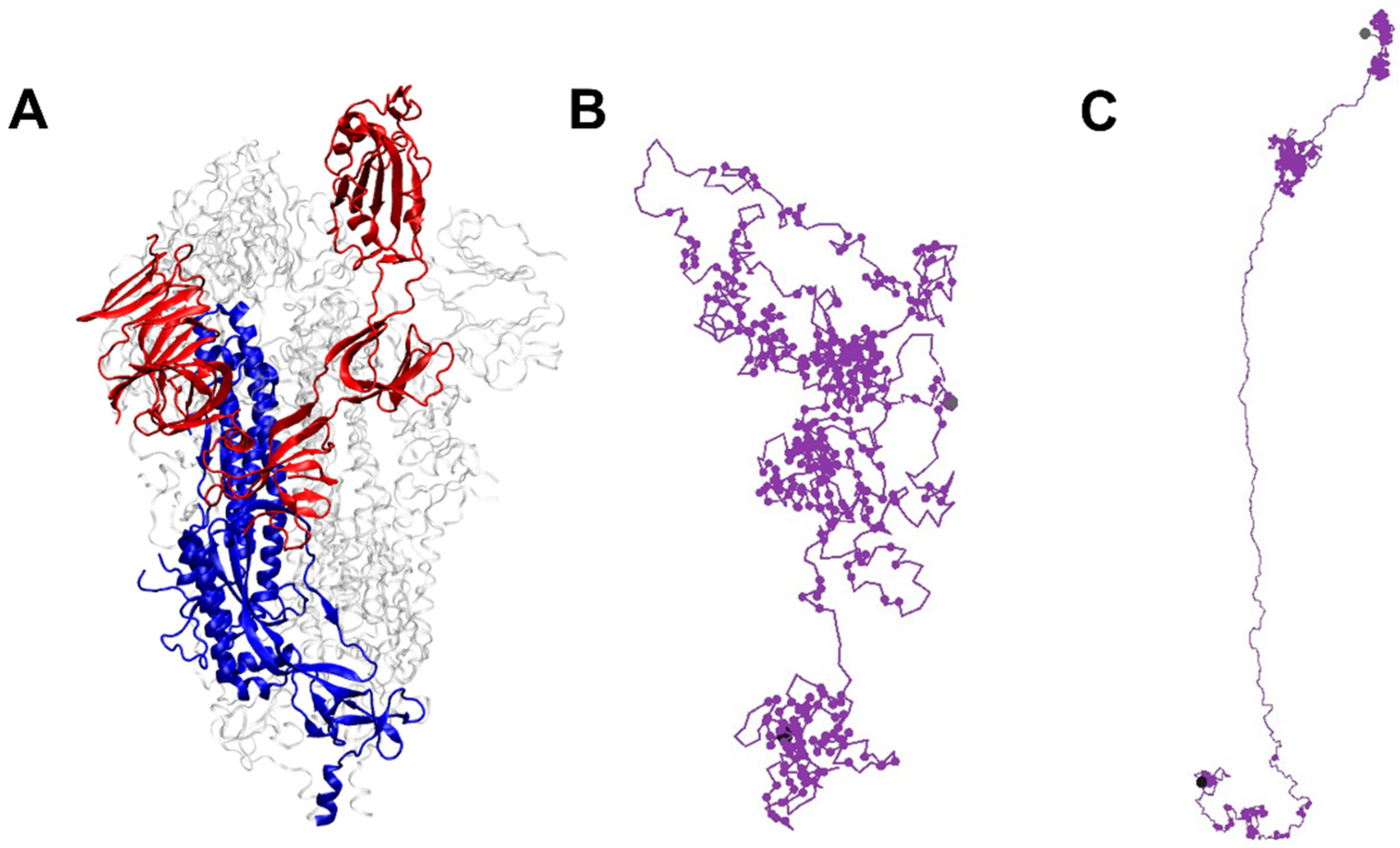A set of typical snapshots of proteins S1 and S2 at the temperature T = 0.0230 is presented in Figure 1. Contrasts in distributions of contacts along the backbone of the proteins S1 and S2 are clearly seen in these snaps: a large fraction of residues in S1 is aggregated throughout into different segments in clusters along its contour leading to a distributed segmental globularization. Relatively, a small fraction of residues participates primarily in two sections towards the tail along the backbone of the protein S2, with a high density of coagulated residues segregated into compact globular segments and a small degree of contacts in segments towards its first residue.

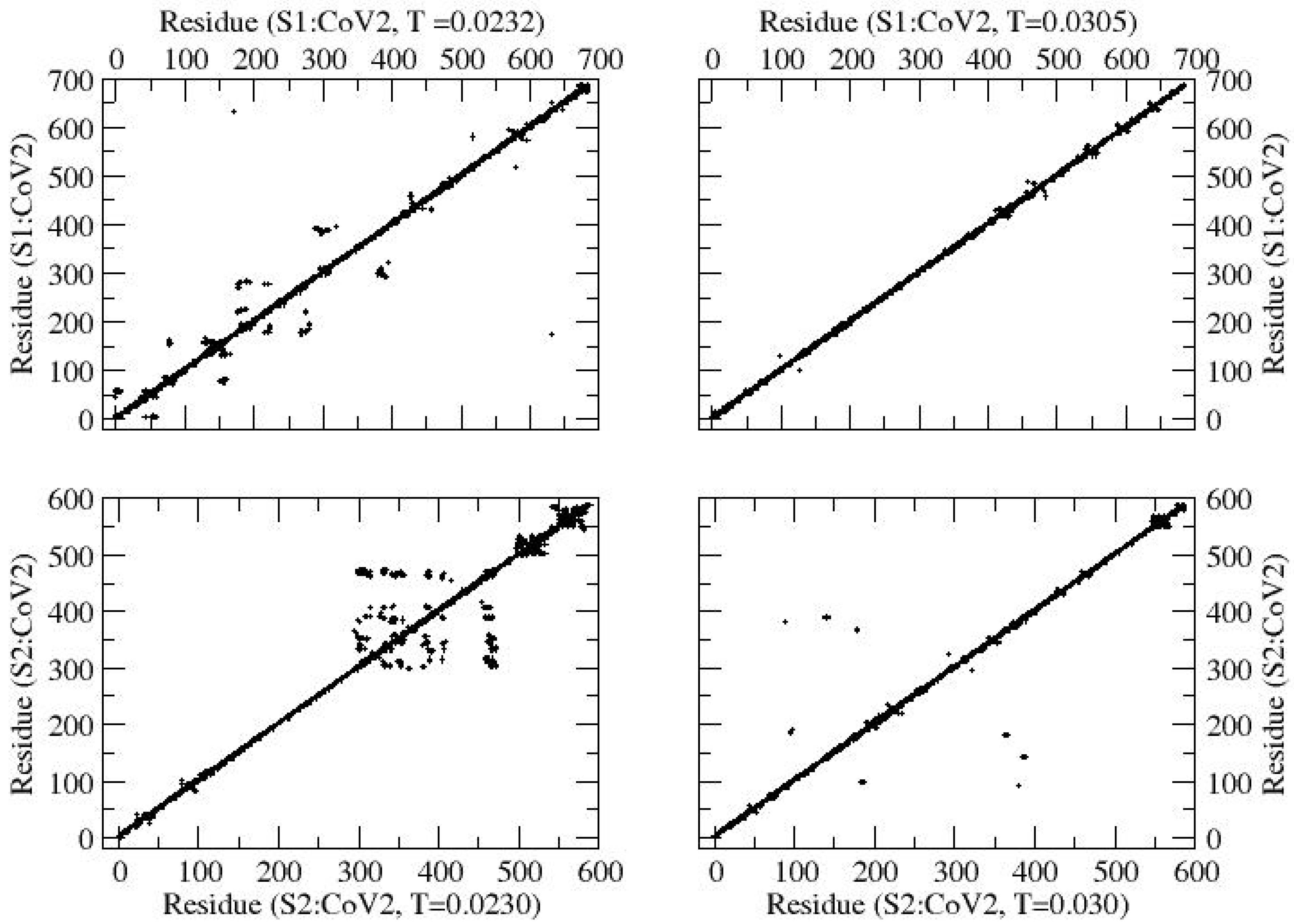
The contact maps (Figure 2) at representative (low and high) temperatures reveal that segmental globularization occurs along the entire backbone of S1 at T = 0.0232. However, the degree of globularization (measured by the density of aggregated residues) decreases considerably on raising the temperature (T = 0.0305). In contrast, segmental globularization in S2 appears localized to specific regions of the backbone. The loops associated with segmental aggregation become larger at a higher temperature (i.e., T = 0.0300). Since snapshots of the protein can vary over time during the course of its structural evolution, they may not be as reliable as quantities averaged over a large fraction of the ensemble. To our knowledge, there are no prior studies directly reporting the contact maps of the individual S1 and S2 subunits; thus, the present results serve as a baseline computational reference for their comparative thermal behavior. Therefore, it is important to analyze the contact profiles by examining the average contact number (N_n) of residues around each across a large number of configurations. For example, configurations in the last one-third time series of the MC steps can provide a reliable average.

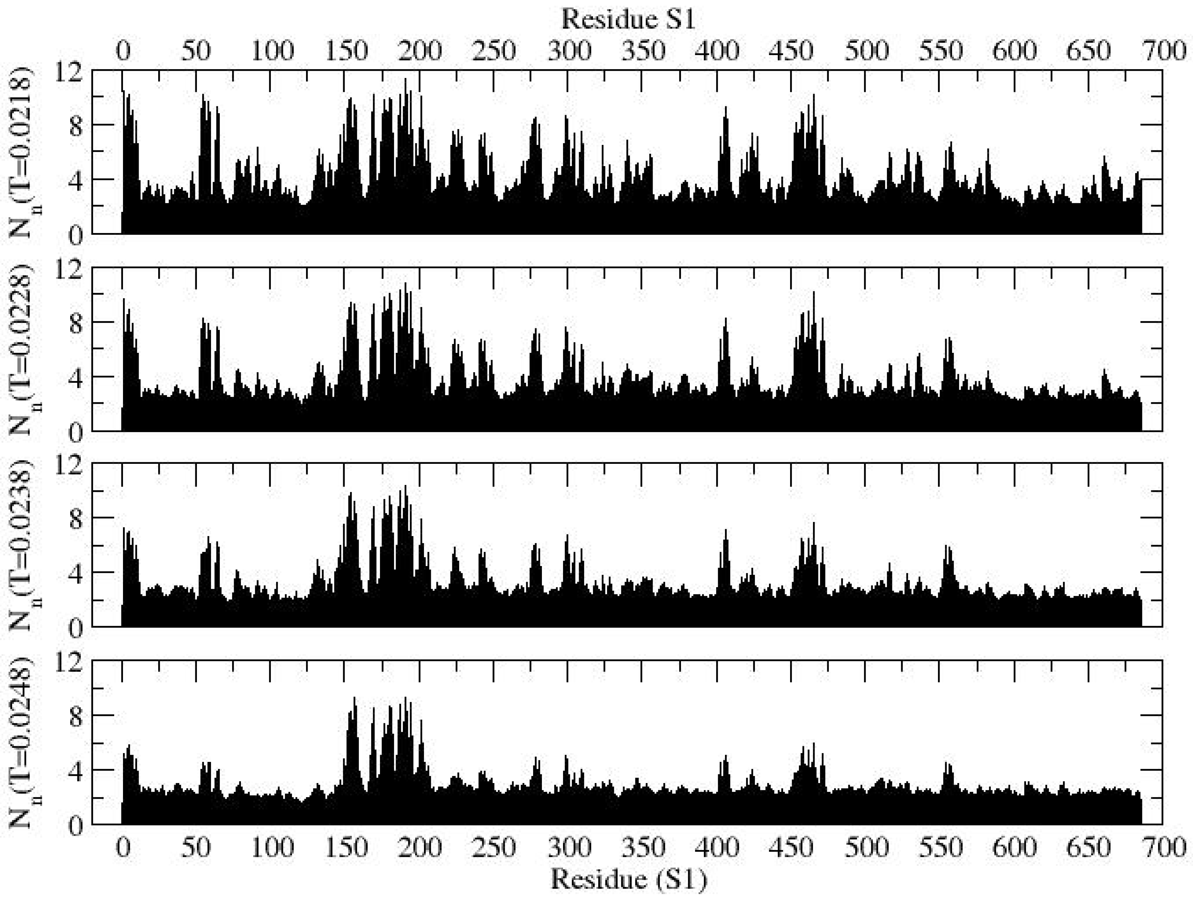
Variability in segmental assembly and re-organization can be assessed by examining the contact profile over a range of temperatures. Figure 3 presents the contact profiles of protein S1 at several representative temperatures. A higher magnitude of contacts (N_n) indicates a higher probability of segmental globularization. 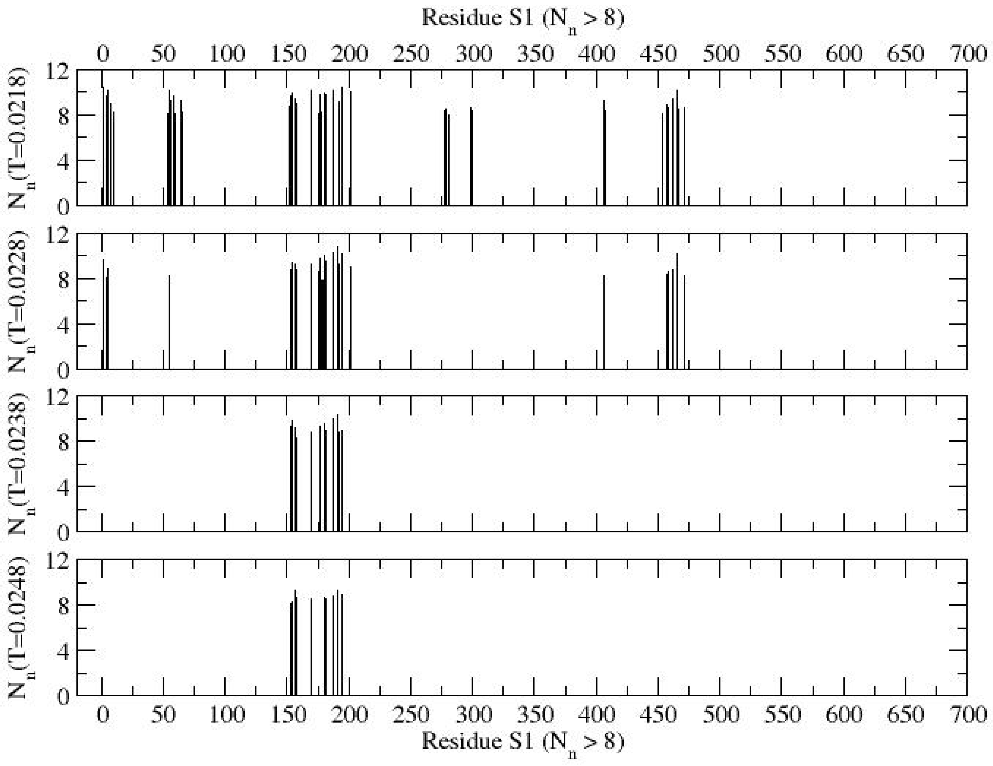Here, "low contact" corresponds to N_n ≈ 0, while "high contact" corresponds to N_n values approaching 10. To clearly identify specific residues with higher globularities, a filtered contact profile showing higher contacts (N_n > 8) is provided in Figure 4. At a low temperature (T = 0.0218), segmental globularization is more prominent in the N-terminal domain (residues Q14–S305), particularly around residues M153–K202, where dominant globularization centers around residues E180, K187, E191, and K195, with an average contact number of N_n = 10. The persistent active segment around M153–K202 in the NTD could be a promising target for drug design aimed at preventive measures. Notably, a large fraction of the residues involved in this segmental globularization is composed of electrostatic residues (D, E, K, R), interspersed with hydrophobic (i.e., M153, M177) and aromatic (F157, F192, F194, W152, Y170) residues. Additionally, a smaller segment of the protein L54-F65 shows significant contacts at the low temperature (T = 0.0218). As the temperature increases, most segmental globularization unravels, with the exception of the M153–K195 region, which remains intact (see Figure 4). In the receptor-binding domain (R319–F541), the segment E406–E471 participates in significant globularization at low temperatures (T = 0.0218, 0.0228) but becomes inactive on raising the temperature.

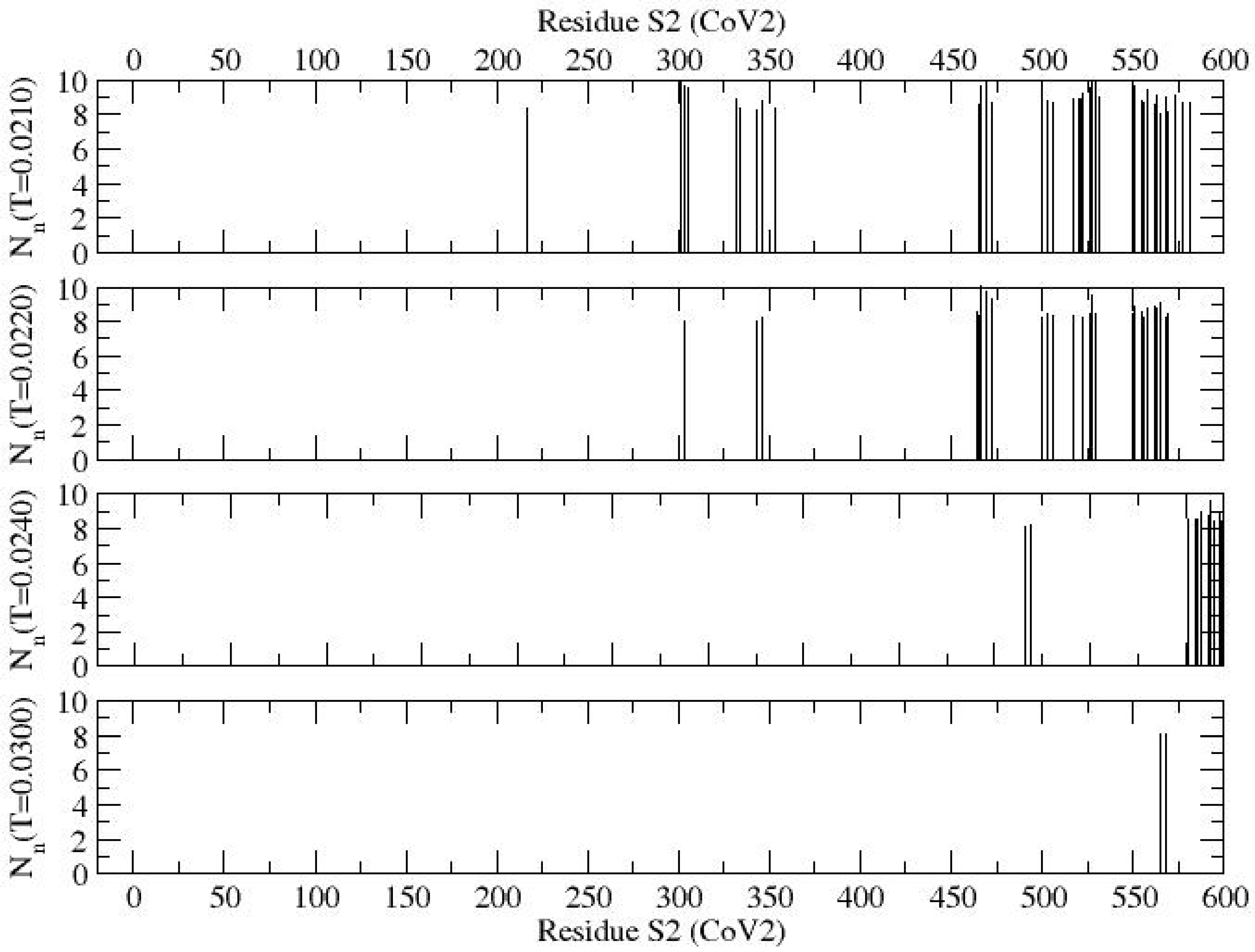
Filtered contact profiles of the S2 segment, focusing on regions with higher contacts, are presented in Figure 5 at representative temperatures of T = 0.0210, 0.0220, 0.0240, and 0.0300, to highlight the variability in segmental assembly. At the low temperature of T = 0.0210, segments with significant contacts are distributed around K986, E988, E990, E1017–K1038, E1150–K1191, and E1202–K1266, with low contact regions interspersed sporadically. As the temperature increases, most of these segmental contacts vanish (see Figure 4). At high temperatures, very few local contacts persist, for example, C1250 and C1253 retain significant contacts at T = 0.0300.

The radius of gyration is a global physical quantity that results from the distribution of cooperative and competing local structures, which are temperature-dependent. The variation in the R_g of the S1 and S2 segments with temperature (T) is presented in Figure 6. A clear contrast in the thermal response of R_g of S1 and S2 is evident, despite the similar number of residues in S1 and S2 (i.e., S1 with 685 residues versus S2 with 588 residues). Notably, the radius of gyration of S2 is significantly larger than that of S1, and the two segments display distinct variation patterns. The radius of gyration of S1 increases (from approximately R_g = 30 to R_g = 45) as the temperature rises (from T = 0.0220 to T = 0.0250), before reaching its steady-state magnitude at high temperatures. In contrast, the R_g of S2 increases dramatically, from about R_g = 30 at a low temperature (T = 0.018) to around R_g = 125 at T = 0.024, and then decreases as the temperature rises further. This non-monotonic thermal response (an initial increase in R_g followed by a decay) appears to be a characteristic of some of the membrane proteins [28]. It is also worth noting that the monotonic increase in the R_g of S1 represents about a 50% rise from its minimum value, whereas the R_g of S2 increases sevenfold (from R_g = 18 to R_g = 125) before decaying to about R_g = 50 at the high temperature of T = 0.037. This striking difference in the thermal responses of S1 and S2 may reflect a unique characteristic of the spike protein associated with COVID-19.

It should be pointed out that Khan et al. [12] reported sporadic changes in R_g of the spike protein S at four temperatures (R_g at T = 0 °C < R_g at T = 20 °C > R_g at T = 40 °C > R_g at T = 60 °C), making it difficult to establish a reliable trend. In our analysis of S1 and S2 here, the R_g of S2 is overwhelmingly dominant over that of S1 and S2 (Figure 6). The limited number of data points on R_g of Khan et al. [12] seem consistent with our observations, i.e., the non-monotonic dependence of R_g (an increase followed by a decrease) on increasing the temperature.

One may study the spread of residues over the length scale λ comparable to the radius of gyration of the protein by evaluating the exponent γ. As mentioned above, the radius of gyration (R_g) is a measure of the average size of the protein conformation. Distribution of the number (N) of residues (N = 685 for S1, N = 588 for S2) over the length scale comparable to the radius of gyration of the protein (λ ~ R_g) can be quantified by estimating its effective dimension D = 1/γ [16]. The effective dimension of the protein spread is a measure of compactness with a higher magnitude of D referring to more compactness.

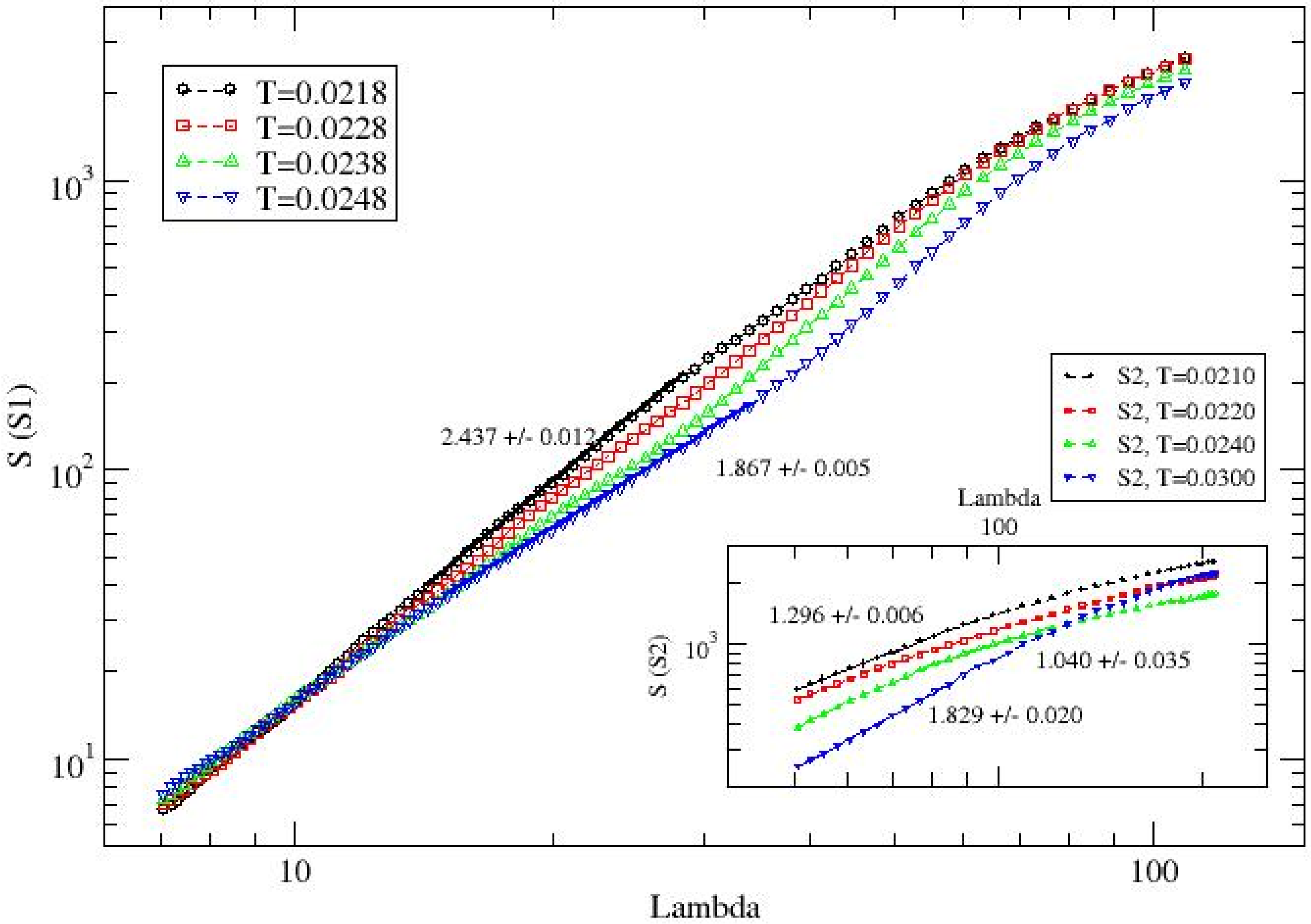
The variation in the structure factor (S(q)) with the wavelength λ, representing the length scale of the protein spread (spanning the radius of gyration) for S1, is presented in Figure 7 at a few representative temperatures, ranging from low to high. The wavelength comparable to the radius of gyration (λ ≈ R_g) corresponds to the overall spread of the protein, while smaller scale data reflect the average spread of shorter segments. The slope of the S(q) vs. λ plot can be interpreted as a measure of the compactness of the protein’s spread across its residues. In scaling analysis of the structure factor, the parameter D estimates the effective dimension of mass distribution, which represents the distribution of residues in systems with heterogeneous mass distribution such as gel. A steeper slope implies a higher degree of compactness or globularization of the protein structure.

Regression analysis of the structure factor data over wavelengths comparable to the radius of gyration for protein S1 shows a systematic decrease in the slope, from approximately D ≈ 2.44 at T = 0.0218 to D ≈ 1.87 at T = 0.0248 (see Figure 7). Similarly, the slopes of the structure factor versus wavelength on a log–log scale for S2 show systematic changes in residue distribution (see inset of Figure 7). For example, D ≈ 1.3 at T = 0.0210 and increases to D ≈ 1.8 at T = 0.0300. Note that while the radius of gyration for S2 remains of the same order of magnitude at both low (T = 0.0210) and high (T = 0.0300) temperatures, the value of D differs significantly: D ≈ 1.296 at T = 0.0210, where the conformation of the S2 is almost linear (fibrous) compared to D ≈ 1.829 at the high temperature of T = 0.0300. This suggests that despite the similar overall spread, the residue distribution at T = 0.0300 may result in a conformation with larger loops than that at T = 0.0210. The temperature dependence of the structure factor reflects intrinsic conformational differences between S1 and S2 rather than model artifacts. Because the residue–residue interaction potential is temperature-independent in our simulations, the observed variations in $S\left(q\right)$ and the effective dimension $D$ arise from the specific sequence composition and contact organization of each subunit.

4. Discussion

At a low temperature (T = 0.0218), the segmental globularization appears to be distributed more in the N-terminal domain (residues Q14–S305) with the most significant around residues M153–K202, where dominant globularization center around residues E180, K187, E191, and K195 with an average contact of about N_n = 10. Note that a large fraction of residues for the segmental globularization contain electrostatic residues (D, E, K, R) with interspersed hydrophobic (i.e., M153, F157, M177, F192, F194) and polar (W152, Y170) residues. A small segment of the protein L54-F65 also has significant contacts at the low temperature (T = 0.0218). Most of the segmental globularization unravels on raising the temperature while keeping the section (M153–K195) intact. Of the receptor-binding domain (R319–F541), the segment E406–E471 participates in significant globularization at low temperatures (T = 0.0218, 0.0228) and becomes inactive on raising the temperature.

In the self-assembly of the protein S2, segments with significant contacts are distributed around K986, E988, and E990 of heptapeptide repeat sequence 1 (HR1), E1017–K1038, E1150–K1191 (part of heptapeptide segment 2, HR2), and E1202–K1266 (including transmembrane (TM) domain and part of the cytoplasm domain) at low temperature (i.e., T = 0.0210); low contact segments are interspersed sporadically in these segments. Very little local contacts persist at high temperature with the exception of residues C1250 and C1253 which retained significant contacts at T = 0.0300.

Despite the comparable number of residues in both proteins S1 (685) and S2 (588), the radius of gyration shows dramatic change in their thermal response. First, the radius of gyration of S2 is considerably larger than that of the S1 with very different variation patterns. The radius of gyration of S1 increases (roughly from R_g = 30 to R_g = 45) on increasing the temperature (T = 0.0220 to T = 0.0250) before reaching its steady-state magnitude at high temperatures. The monotonic increase in R_g of S1 is about 50% of its minimum magnitude. The radius of gyration of S2 increases from about R_g = 30 at low temperature (T = 0.018) to about R_g = 125 around T = 0.024, a 7-fold increase with the temperature, before decaying down to about R_g = 50 on further increasing the temperature, i.e., T = 0.037. The non-monotonic thermal response (increase in R_g followed by decay with the temperature) of S2 appears to be a characteristic of some of the membrane proteins. The relatively large magnitude of R_g variations reflects the coarse-grained nature of the model, which amplifies relative fluctuations to highlight the qualitative thermal trends rather than exact experimental magnitudes. Our analysis therefore focuses on the comparative behavior of S1 and S2, not on reproducing absolute experimental values. Part of the non-monotonic response of R_g of the spike protein may be consistent with a limited number of data points by Khan et al. [12]. That such a dramatic contrast in the thermal response of S1 and S2 may be due to the specific characteristics of the spike protein associated with COVID-19 should be worth pointing out.

The effective spread of the proteins (S1, S2) is quantified by a scaling analysis of the structure factor (S(q)) with the wave vector by estimating their effective dimension, a measure of globularity. The effective dimension (D) of the protein S1 decreases from about D ~ 2.44 at T = 0.0218 to D ~ 1.87 at T = 0.0248; a higher magnitude of D reflects a higher degree of compactness or globularity. The globularity index of S2 remains low: D ~ 1.3 at T = 0.0210 and about D ~ 1.8 at T = 0.0300. Note that the radius of gyration of S2 is of the same order of magnitude both at low (T = 0.0210) and high (T = 0.0300) temperatures. Note the difference in magnitude of D, i.e., D ~ 1.296 at T = 0.0210 (low temperature) where the conformation of the protein S2 is almost linear (fibrous) with that at the high temperature T = 0.0300 with D ~ 1.829 (with lower R_g), which suggests that the conformation of the protein S2 may have a larger loop (despite the same overall spread (R_g)).

The present coarse-grained lattice model differs substantially from the simplified lattice models used in early studies. It extends the bond-fluctuation mechanism on a regular cubic lattice, providing sufficient degrees of freedom to capture both local and global conformational responses under varying thermal conditions. This method has been widely and successfully applied to polymers, peptides, and complex biomolecular systems [26]. The use of a lattice representation is primarily for computational efficiency without compromising thermodynamic accuracy. Although the SARS-CoV-2 spike protein does not undergo sharp conformational transitions like folding–unfolding events, our focus is to probe the differential thermal responses of its S1 and S2 subunits. The distinct behaviors observed here demonstrate that this approach effectively captures those variations within the accessible thermal regime.

Although the present coarse-grained approach employs the same theoretical framework as our previous study on the CorA protein [28], the systems investigated here are structurally distinct. The S1 and S2 subunits of the SARS-CoV-2 spike protein differ substantially in residue composition, topology, and sequence organization, leading to markedly different conformational and thermal responses. The contrasting behaviors observed in Figure 6 therefore arise from the intrinsic structural characteristics of S1 and S2 rather than from artifacts of the computational model.

It should be noted that our analysis relies solely on coarse-grained simulations without direct experimental validation. While such computational approaches are valuable in identifying general trends and generating mechanistic hypotheses, the absolute quantitative values should be interpreted with caution. These findings thus provide qualitative insights into the contrast in the local and global structural dynamics of S1 and S2.

5. Conclusions

We have thus systematically analyzed the thermal response of the spike protein components S1 and S2 from SARS-CoV-2 using coarse-grained simulations. The results reveal distinct conformational behaviors; S1 exhibits a monotonic dependence of the radius of gyration (a continuous increase towards its saturation) with the temperature, while S2 shows a non-monotonic thermal response, characterized by an expansion followed by contraction with the temperature. These findings highlight the contrasting segmental reorganization and globularization patterns of the two proteins: S1 becomes increasingly compact and S2 displays fibrous characteristics that evolve with temperature. Our scaling analysis further shows that the effective dimension of residue distribution (D) for both proteins varies with temperature, reflecting changes in their structural compactness and organization. It is noted that residues in the NTD (Q14–S305, with a focus around M153–K202) exhibit significant globularization, suggesting a potential target region for drug design. These thermal dynamics of S1 and S2 may provide valuable insight into designing antiviral strategies targeting the structural stability of SARS-CoV-2 spike proteins.