Article

Estimation of Growth Parameters of Eustoma grandiflorum Using Smartphone 3D Scanner

1
Graduate School of Agricultural and Life Sciences, The University of Tokyo, 1-1-1 Yayoi, Bunkyo 113-8657, Tokyo, Japan
2
Tohoku Agricultural Research Center, National Agriculture and Food Research Organization, 50 Harajuku Minami, Arai, Fukushima 960-2156, Fukushima, Japan
*
Author to whom correspondence should be addressed.
Eng 2025, 6(9), 232; https://doi.org/10.3390/eng6090232 (registering DOI)
Submission received: 30 July 2025 / Revised: 27 August 2025 / Accepted: 28 August 2025 / Published: 5 September 2025

Abstract

Since the Great East Japan Earthquake, floriculture has expanded in Namie Town, Fukushima Prefecture, as part of agricultural recovery. Growth surveys are essential for floriculture production, cultivation management, and trials as they help assess plant growth. However, these surveys are labor-intensive, and the standards used can vary owing to subjective judgments and individual differences. To address this issue, image-processing technologies are expected to enable more consistent and objective evaluations. In this study, we explored image processing in growth surveys by estimating plant growth parameters from three-dimensional (3D) point clouds acquired using a smartphone-based 3D scanner. Focusing on lisianthus (Eustoma grandiflorum), we estimated the plant height and the number of nodes above the bolting. The results showed that plant height could be estimated with high accuracy, with a root mean square error (RMSE) of 1.2 cm. By contrast, the node number estimation showed a mean error exceeding one node. This error was attributed to the challenges in handling variations in point cloud density, which stem from the 3D point cloud generation method and leaf occlusion caused by dense foliage. Future work should focus on developing analysis methods that are robust to point-cloud density and capable of handling complex vegetative structures.

1. Introduction

Since the Great East Japan Earthquake, flower cultivation has been expanding in Namie Town, Fukushima Prefecture, as part of agricultural reconstruction efforts [1]. Lisianthus is the main crop, has the highest unit price among cut flowers, and supports the income of flower growers. In the cultivation of flowers and plants, growth surveys are conducted to investigate the plant growth conditions. Currently, prefectural researchers, extension advisors, and willing growers conduct growth surveys. The purposes of growth surveys vary from introducing new technology to understanding current growth conditions and comparing fields. Such surveys provide results that constitute indispensable information for addressing critical challenges in agriculture, including adaptation to climate change through the adoption of new technologies, yield improvement by monitoring current growth conditions, and mitigation of labor shortages through the support of novice farmers. However, current growth surveys are labor-intensive and subject to errors owing to misjudgment and individual differences.
Therefore, image-processing technology is expected to be utilized in growth surveys. In previous studies, many automatic measurements of plant growth parameters were conducted using image processing technology [2]. These studies primarily used 2-D and 3-D measurements, which differ in terms of the information obtained, cost, and measurement time. For example, in a study on sweet potatoes, the number of leaves, plant height, and leaf area were analyzed using 2D images and 3D point clouds generated using the structure from motion (SfM) technique, and the results using 3D point clouds showed higher accuracy [3]. This is attributed to the fact that errors caused by shading and distance are unavoidable in 2D images. Therefore, more accurate growth parameters can be obtained using 3D measurements. Additionally, research on growth surveys using 3D measurements is currently underway: for example, node detection and internode length measurement of cucumbers [4], extraction of corn stem height using depth sensors [5], and estimation of the leaf area density and leaf area index of tomatoes using portable LiDAR [6]. However, the sensor equipment used for 3D measurements is expensive, and its introduction into the field poses a challenge. Research using Kinect is a relatively inexpensive method for 3D measurements. For example, some studies photographed individual tomatoes in a greenhouse [7] and potted lettuce [8], estimated the stem diameter of bananas [9], and evaluated the growth and yield of cauliflowers [10]. However, the resolution of Kinect is limited when the object and the area to be photographed are large. Several previous studies on SfM generated a 3D point cloud from multiple 2D images as a method of acquiring a 3D point cloud without using expensive equipment. For example, multiple plant seedlings were photographed indoors using a single-lens reflex camera to obtain and analyze a 3D point cloud [11], tomato seedlings were photographed using a multiview camera to segment a 3D point cloud [12], and cotton plants were photographed from a moving platform on the ground to reconstruct a 3D point cloud [13]. However, these studies require the use of a camera to capture many images, and practical problems arise, such as the time and effort required to process them. Against this background, a method was proposed to estimate the growth parameters by constructing a 3D point cloud from videos captured using a smartphone [14]. However, this method requires time-consuming processing to generate a dense point cloud using SfM from video images. Approximately 1 h of processing is required to generate a point cloud, which is unsuitable for cases in which the results need to be verified immediately in the field. A previous study [15] used neural radiance fields (NeRFs) to perform 3D reconstruction from images captured with a smartphone; however, the detection of rice and 3D reconstruction were performed on a PC, and the acquisition of the 3D point cloud was not completed on the smartphone.
Today, technology that enables real-time acquisition of 3D point clouds via smartphone applications has emerged, and research into their use has begun. For example, a smartphone application has been used to evaluate the leaf area and transpiration of corn [16]. Research focusing on 3D measurement of flowers is limited. Some studies have been conducted, for example, on the acquisition of 3D point clouds of roses using X-ray CT [17] and the use of Kinect to capture and analyze 3D point clouds of Chinese Cymbidium [18]. In the case of lisianthus, existing studies are limited to investigations of the relationship between corolla formation and cell enlargement [19] or simulations of flowering using 3D meshes [20]. To the best of our knowledge, there are no reports of 3D measurements that can be used to investigate the growth of lisianthus. In addition, differences in plant morphology, scale, measurement items, and imaging methods make it uncertain whether existing approaches can be directly adapted to the practical growth surveys carried out in Fukushima, highlighting the need for further investigation.
Therefore, this study examined the possibility of conducting a growth survey using 3D point clouds obtained from a smartphone 3D scanner for lisianthus, a major floricultural product. Several growth survey items for lisianthus used in Fukushima, including plant height and the number of nodes above the bolting, which indicates the growth stage, are important for understanding the growth condition at each stage and for irrigation management. In particular, the number of nodes above the bolting is dependent on the morphology of lisianthus and exhibits characteristic counting features. Therefore, in lisianthus cultivation, we focused on plant height and the number of nodes above the bolting and evaluated the accuracy of their estimation. This study represents a novel approach by targeting lisianthus, a floricultural species that has been scarcely investigated using 3D measurement techniques, and by focusing on growth survey parameters that are directly relevant to practical field management.

2. Materials and Methods

2.1. Plant Materials and Cultivation Conditions

The plants were grown in a greenhouse (frontage: 5.4 m; depth: 12.5 m; eaves height: 2.8 m) at the Fukushima Research Station, Tohoku Agricultural Research Center, National Agriculture and Food Research Organization, Fukushima City, Fukushima Prefecture, Japan (36°42′ N, 140°23′ E). Celled seedlings of lisianthus (Eustoma grandiflorum (Raf.) Shinn.), varieties ‘Celebritch White’ (C) and ‘Happiness White’ (H), were purchased and transplanted into No. 8 root pots (Yamato Plastic, Nara, Japan) on 5 April 2024. Each pot (4.8 L) was filled with 4.66 L of a commercial growing medium (Arrenza Holdings Corporation, Fukushima Prefecture; high-grade medium for flowers and vegetables) containing a base fertilizer and supplemented with 0.14 L of granular fertilizer (Genki Kun No. 1, Katakura Co-op Agri Corporation, Tokyo, Japan). Irrigation was performed manually by using a hose reel. In the early growth stage, watering was applied once every 1–3 d. At the mid-stage, watering was adjusted to allow for sufficient drainage, and after bud emergence, irrigation was applied to prevent wilting. Apical flowers were removed immediately after bud formation to promote the growth of the lateral branches. The lateral shoots arising from the lower nodes were removed at an early stage. On 30 July, at peak flowering, the plants were adjusted to maintain three flowers and three buds per plant. Foliar fertilization was performed using Kumiai Organic Tomy Liquid Fertilizer (Katakura Co-op Agri Co., Ltd., Tokyo, Japan) diluted 1:1000 to prevent nutrient deficiency. The temperature was maintained as required by opening and closing the side windows and operating a gable-end fan for ventilation. The average daily temperature during the cultivation period was 28.6 °C.

2.2. Growth Survey and Definition of Target Growth Parameters

Four plants from each of the two lisianthus (Eustoma grandiflorum) varieties were selected for evaluation. To assess the accuracy of point-cloud-based estimations, a growth survey was conducted, including measurements of plant height and the number of nodes. The survey protocols followed the standard guidelines used in the official survey of Fukushima Prefecture. Plant height, as shown in Figure 1, was defined as the vertical distance from ground level to the highest point of the plant and was measured using a ruler. Plant height serves as an indicator of growth vigor and is a critical factor in determining the shipping grade of cut flowers. Bolting was defined by the presence of internodes spaced at least 1 cm apart. The number of nodes above the bolting was visually counted. Because lisianthus exhibits opposite phyllotaxy, only nodes with fully developed leaves were included in the count. The number of nodes is considered an indicator of the developmental stage, which is crucial for cultivation management. In particular, night temperatures and irrigation schedules must be adjusted according to the growth stage of the plant.

2.3. Three-Dimensional Data Acquisition Using Smartphone Application

The 3D data were acquired in the greenhouse where the plants were cultivated using the Scaniverse smartphone application (ver. 3.02). Scaniverse provides two data acquisition modes: “Splat” and “Mesh.” Although the mesh mode offers multiple data formats, the splat mode was selected because of the complex morphology of the target plants. Scaniverse uses Gaussian splicing to reconstruct 3D scenes. Gaussian plating enables faster 3D reconstruction from multiple images compared with conventional methods [21]. Images were captured manually, with the operator holding an iPhone 12 or iPhone 12 Pro smartphone and walking around the plant several times. The built-in camera (f/1.6) of the smartphones was used for imaging. Data acquisition was performed during the daytime under clear conditions to ensure consistent illumination, and the generated 3D models were briefly checked onsite to ensure quality. Data were acquired on 27 May, 14 June, 26 June, 18 July, and 30 July 2024. Among these five dates, only the first three prior to bud emergence were used in the analysis. This is because plant height and the number of nodes above the bolting are key indicators of growth management before bud formation, which was the primary focus of this study. For clarity, 27 May, 14 June, and 26 June are referred to as the early, middle, and late growth stages, respectively. These stages correspond to BBCH codes 41, 43, and 45, respectively [22].

2.4. Estimation of Plant Height from 3D Point Clouds

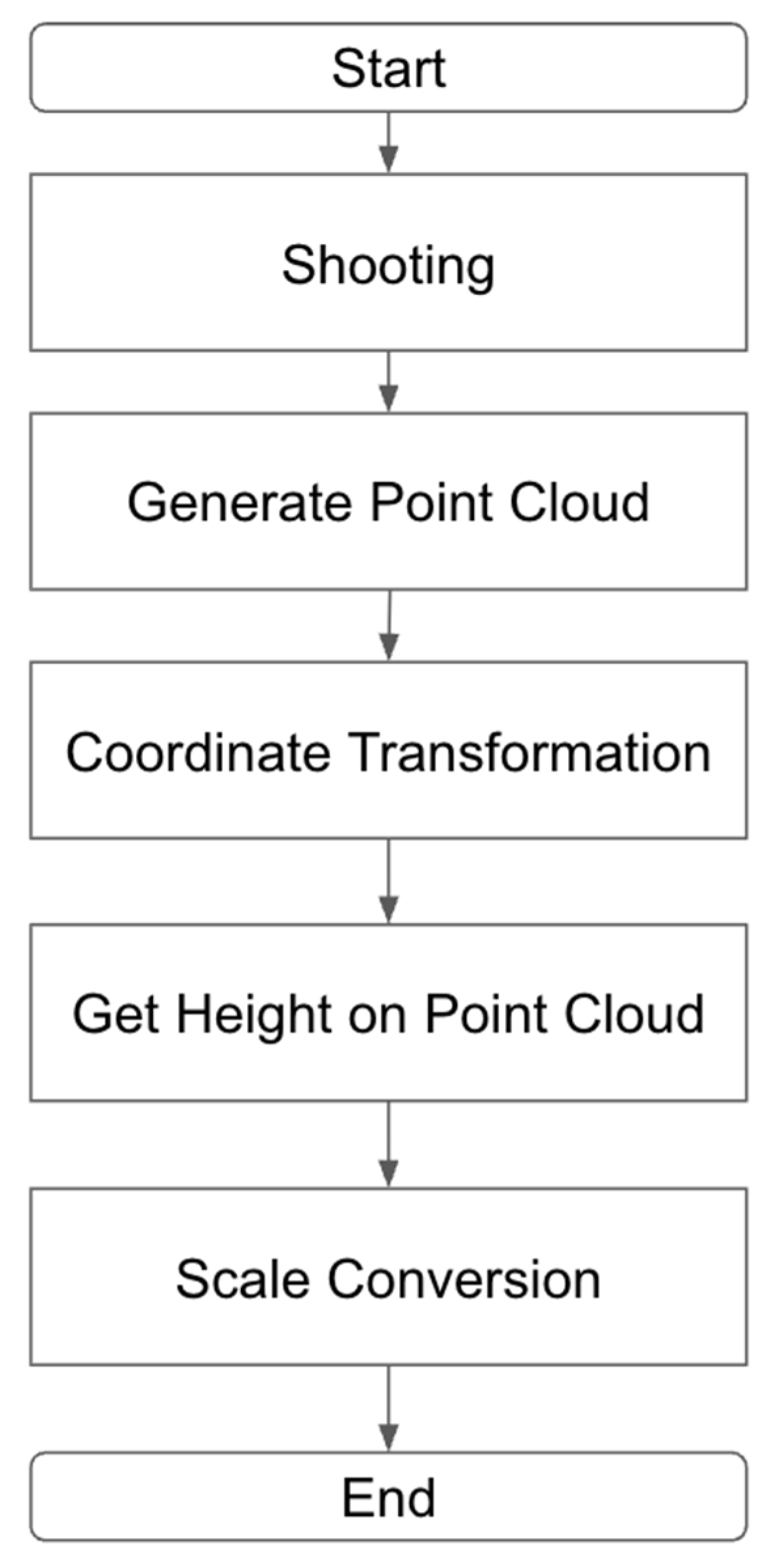
The method used to estimate plant height is shown in Figure 2. First, a ground plane corresponding to the pot surface was detected from the point cloud using a Random Sample Consensus (RANSAC) algorithm. The coordinate system was then transformed based on the estimated plane. Specifically, the point cloud was rotated using Rodrigues’ rotation formula so that the normal vector of the detected plane became parallel to the xy-plane and subsequently translated to align the plane with z = 0. The implementation was performed in Python 3.11.2, using Open3D (version 0.18.0), with a distance threshold of 0.01, three samples, and 1000 iterations as the parameters. After the coordinate transformation, the maximum absolute value of the z-coordinate was extracted as the plant height in the point cloud space. This value was scaled using the known pot height—measured with a centimeter-graduated ruler—to estimate the actual plant height in real-world units.

2.5. Estimation of Number of Nodes Above Bolting from 3D Point Clouds

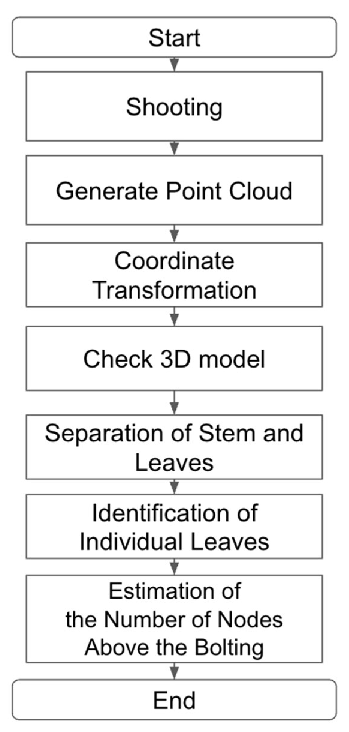
The method used to estimate the number of nodes above the bolting is illustrated in Figure 3. First, the 3D point cloud was visually inspected to confirm the data quality. The same coordinate transformation applied for plant height estimation—namely, rotation using Rodrigues’ rotation formula to align the pot surface with the xy-plane and translation to set the plane at z = 0—was performed to standardize the point cloud orientation. Stem and leaf regions were separated using a custom algorithm. Among the remaining data, only the leaf points were extracted and subjected to clustering to identify individual leaves. Finally, the number of nodes above the bolting point was estimated based on the spatial distribution of the identified leaves.

2.5.1. Point Cloud Segmentation and Node Estimation Accuracy

The acquired 3D point cloud was visually inspected to confirm the absence of missing or corrupted data. Subsequently, the stem and leaf regions were separated by detecting linear structures using the RANSAC algorithm. Consequently, only leaf point clouds were retained. Specifically, we employed the method proposed by Mariga (2022), which was implemented in the open-source pyransac3d library [23]. To evaluate the accuracy of the stem–leaf separation, we used mean intersection over union (mIoU) and accuracy (Acc) as performance metrics. Based on the classification results for each point, the numbers of true positives (TP), false positives (FP), and false negatives (FN) were aggregated. The overall Acc and Intersection over Union (IoU) for each class were calculated using Equations (1) and (2), respectively. The mIoU was then computed as the average of the IoUs across all the classes.
A c c = T P ( T P + F P + F N )
I o U = T P T P + F P + F N

2.5.2. Leaf Clustering and Node Count Estimation

Subsequently, individual leaves were identified using the Density-Based Spatial Clustering of Applications with Noise (DBSCAN) algorithm [24], which clusters the points corresponding to each leaf. In this study, the distance threshold parameter was set to 0.035, and the minimum number of points per cluster was set to 10. These parameters were determined based on the density distribution of the original point cloud. To evaluate the accuracy of leaf identification, all the identified leaves were visually inspected using a 3D model to determine whether clustering was successful. The nodes on the plant stem were numbered sequentially from the base upward, and the success rate of leaf identification was aggregated per node and plotted on a graph. Furthermore, nodes were divided into three groups—upper, middle, and lower thirds—based on the total number of nodes per plant, and identification success rates were calculated for each group based on the acquisition date. Finally, the number of nodes above the bolting was estimated based on the vertical coordinate information. Leaves with the nearest distance to the ground below a certain threshold were excluded; this threshold was set to 0.01 in point cloud units, corresponding approximately to 1.2 cm after scaling to real-world measurements considering pot size. Because lisianthus exhibits the opposite phyllotaxy, with two leaves per node, nodes were inferred by grouping leaves whose vertical positions were within a specified distance from each other. In this study, leaves with vertical distances of less than 0.01 in point cloud space (approximately 1.2 cm in real scale) were treated as belonging to the same node, and the total number of nodes was estimated accordingly.

2.6. Evaluation of Estimation Accuracy

Scatter plots of the measured versus estimated values were generated to evaluate the accuracy of the estimated plant heights and node counts. The goodness of fit of the regression line was assessed using the coefficient of determination (R2). Additionally, two evaluation metrics were employed to quantify the estimation accuracy: root mean squared error (RMSE) and mean absolute percentage error (MAPE). The RMSE indicates the average magnitude of the error, including variance, whereas the MAPE represents the relative size of the error with respect to the measured values. Together, these metrics provide an assessment of the absolute and relative differences between the measured and estimated values. RMSE and MAPE are defined by Equations (3) and (4), respectively, where y i , y ^ i , and n denote the measured, estimated, and total number of samples, respectively.
R M S E = 1 n i = 1 n ( y ^ i y i )
      M A P E = 100 n i = 1 n y ^ i y i y i

3. Results

3.1. Estimation of Plant Height
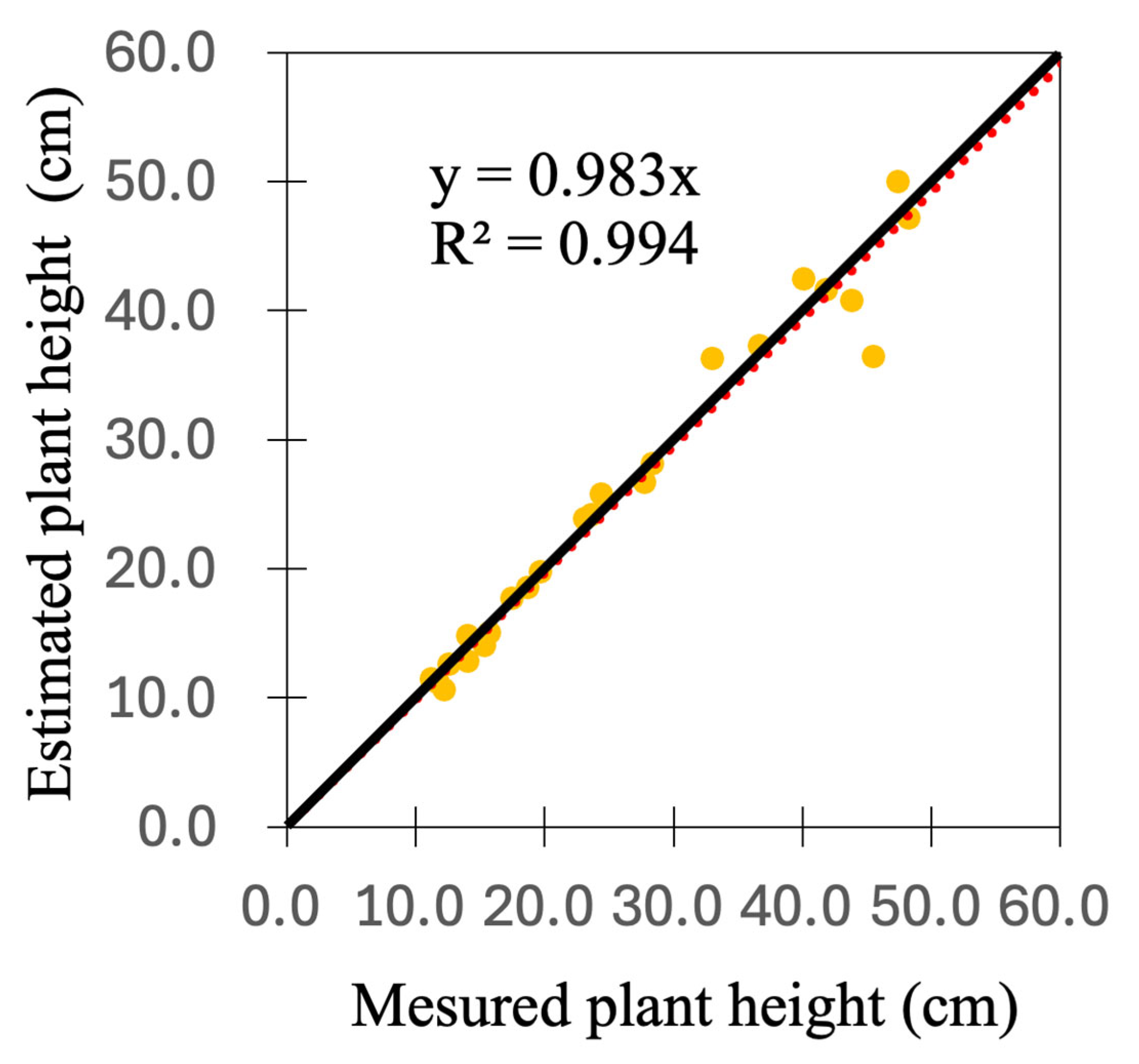
Figure 4 illustrates the relationship between the measured and estimated plant heights. The estimated values closely matched the measured values with no apparent outliers. RMSE was 1.2 cm, indicating a small average estimation error. The coefficient of determination was 0.994, indicating a strong fit to the regression line. A correlation test between the estimated and measured values yielded a p-value of 1.0 × 10⁻¹⁷, confirming a statistically significant correlation at the 1% significance level.
Table 1 summarizes the estimation accuracy of plant height at different growth stages. RMSE and MAPE were calculated for each stage to evaluate variations in measurement accuracy during development. The results showed that estimation errors were generally small and stable, although slight variations were observed depending on plant morphology. At the Late stage, the RMSE increased to 3.8 cm compared with other stages. However, the MAPE remained at 6.9%, showing only a small difference from other stages. This indicates that although the absolute error increased as the plants grew, the relative accuracy was maintained.
Figure 4. Relationship between measured and estimated plant height (the solid line represents y = x; the red dashed line represents y = 0.98x). The yellow dots indicate the correspondence between each measurement and the actual plant height.
Eng 06 00232 g004
Table 1. Plant height estimation accuracy across growth stages.
RMSE (cm)MAPE (%)
Early1.05.0
Middle0.74.5
Late3.86.9
All1.25.3

3.2. Separation of Stem and Leaf

Figure 5 presents an overview of the original point clouds obtained using Scaniverse (a–c) and the results of the stem–leaf separation performed using the RANSAC algorithm (d–f). Overall, the stem and leaf regions were separated with a relatively high accuracy. However, during the middle growth stage, some leaf tips were mistakenly classified as stems. Table 2 summarizes the quantitative evaluation of stem–leaf separation accuracy using the RANSAC method. Both the mIoU and Acc were high, confirming the effective separation of the stems and leaves. When analyzed according to growth stage, the late stage tended to exhibit the highest accuracy values. Furthermore, the organ-specific evaluation revealed that the IoU for leaves was higher than that for stems.

3.3. Identification of Individual Leaves
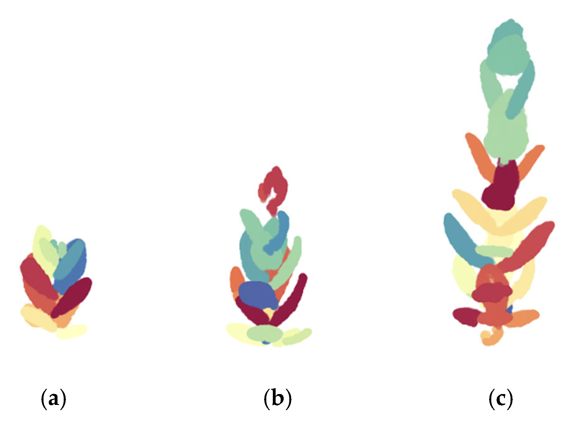
Figure 6 illustrates the clustering results. Overall, the individual leaves were successfully identified; however, some regions exhibited inaccurate leaf segmentation. Table 3 presents the identification success rates for each plant region. Across all observation periods, the middle nodes exhibited higher identification success rates than the upper and lower nodes, where the success rates decreased. When analyzed by acquisition date, the late growth stage tended to have lower overall identification success rates, with the middle nodes particularly exhibiting reduced accuracy.
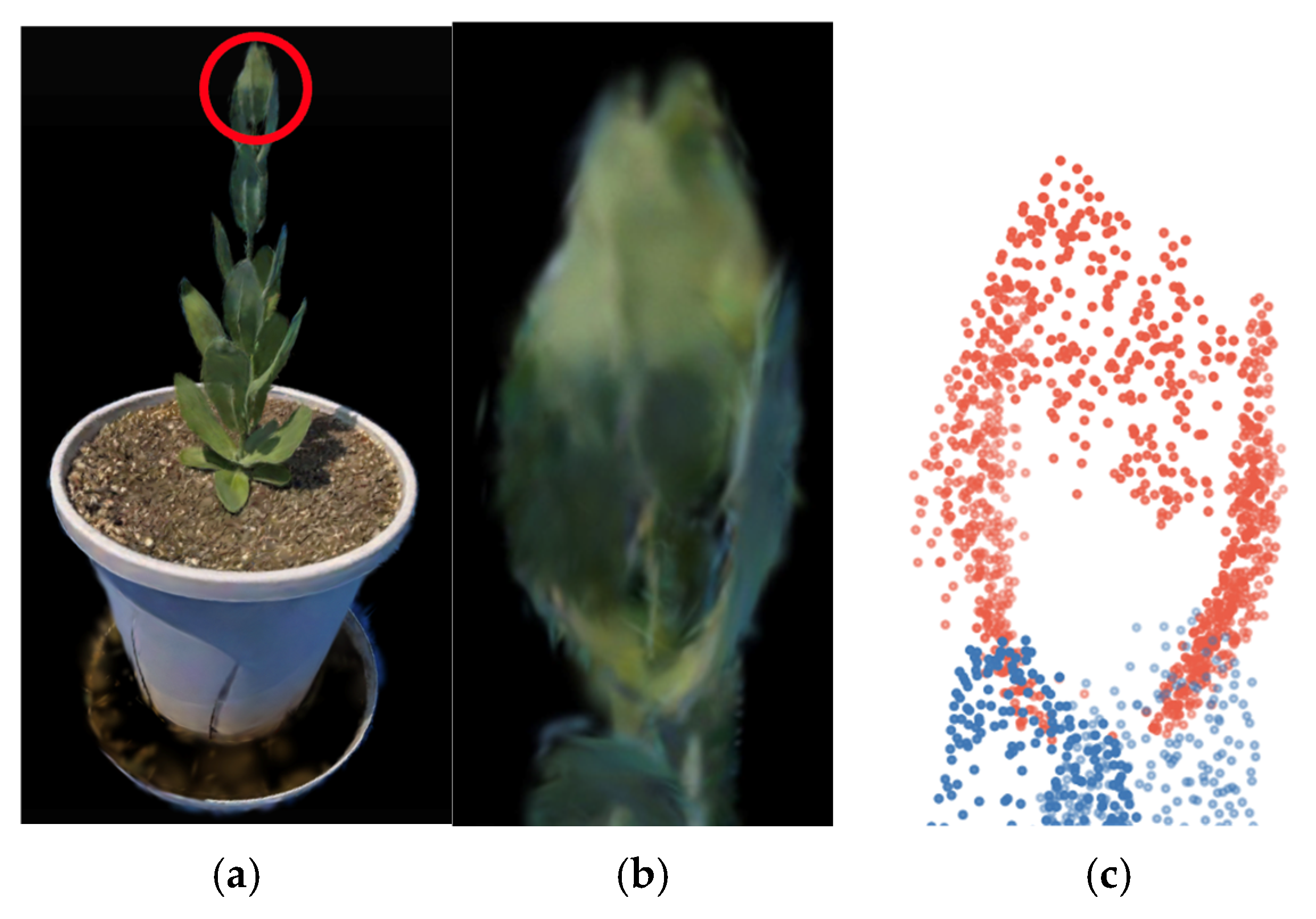
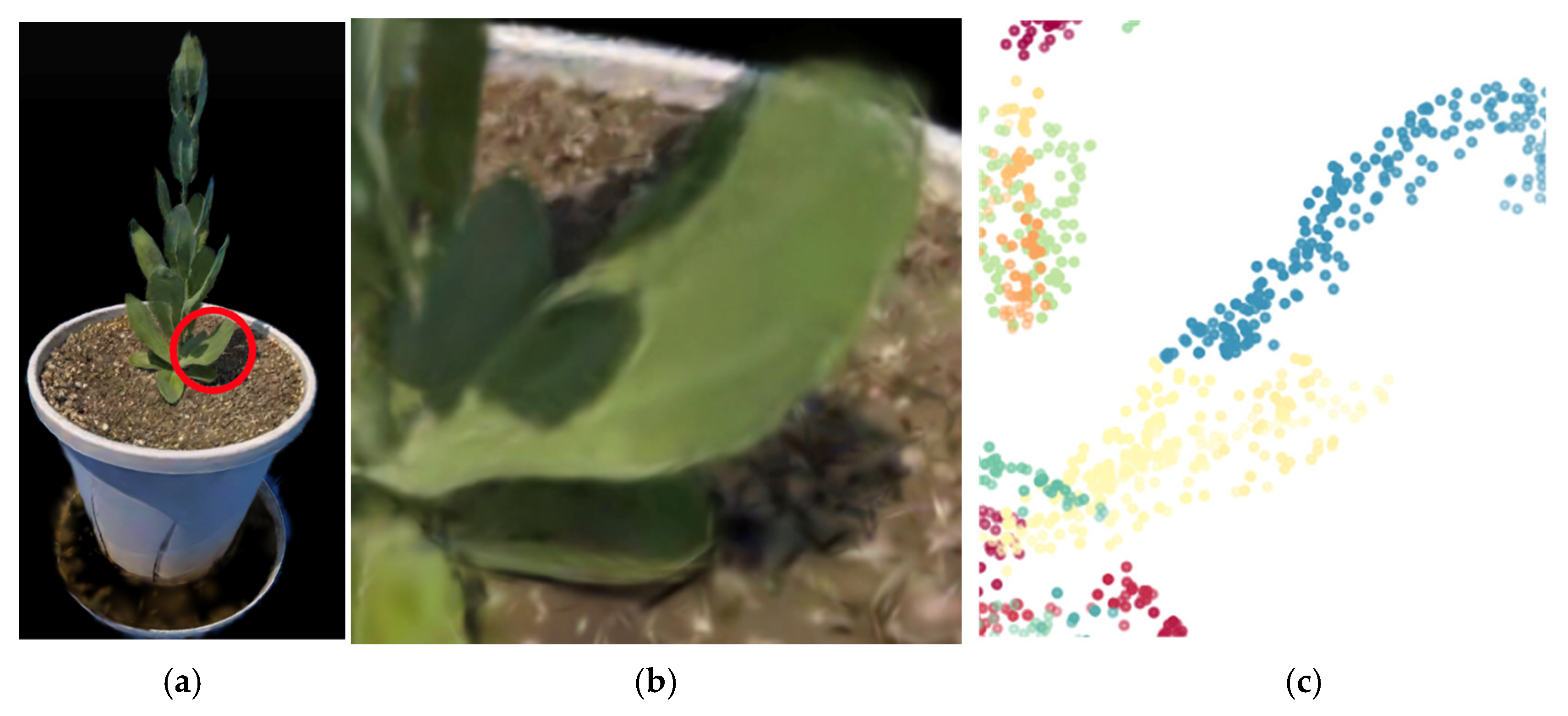
A visual assessment was conducted to investigate the factors contributing to the decline in identification accuracy. Figure 7 depicts a region near the apex where the leaves are densely clustered. Owing to this dense leaf arrangement, individual leaves could not be distinguished correctly; a cluster that should have been identified as four separate leaves was mistakenly classified as a single leaf. Conversely, Figure 8 shows an example in which a single large leaf was erroneously segmented into multiple leaves. This is because the point cloud was sparse in part of the area, leading to one leaf being classified into three separate clusters.
Figure 6. Visualization of individual leaf identification performed using DBSCAN. Different colors indicate different clusters, each corresponding to a separate leaf. (a), (b), and (c) correspond to early, middle, and late growth stages, respectively.
Eng 06 00232 g006
Table 3. Success rate of individual leaf identification by plant part.
Success Rate of Individual Leaf (%)
LowerMiddleUpper
Early677913
Middle629243
Late285834
Figure 7. Example images of misidentifying multiple leaves as a single leaf. (a) shows the original Scaniverse scene of the entire plant, where the red circle highlights the region corresponding to the target scene in (b). (c) presents the result of identification using DBSCAN. In (c), different colors indicate different clusters, each corresponding to a separate leaf.
Eng 06 00232 g007
Figure 8. Example images of misidentifying a single leaf as multiple leaves. (a) shows the original Scaniverse scene of the entire plant, where the red circle highlights the region corresponding to the target scene in (b). (c) presents the result of identification using DBSCAN. In (c), different colors indicate different clusters, each corresponding to a separate leaf.
Eng 06 00232 g008

3.4. Estimation of the Number of Nodes Above the Bolting
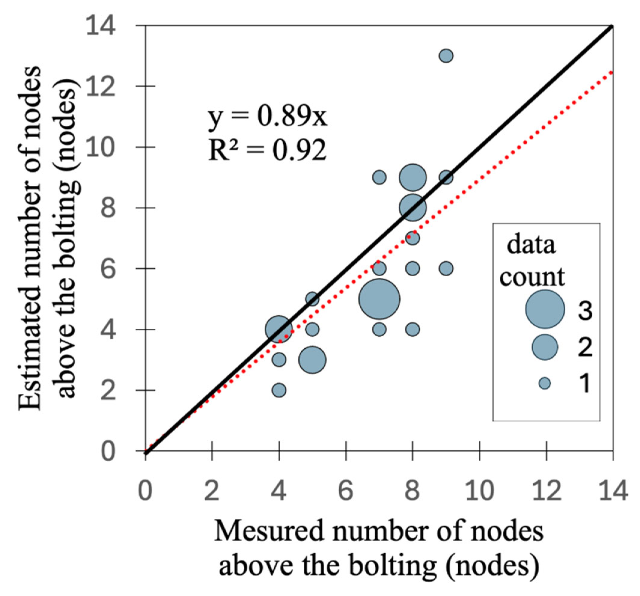
Figure 9 illustrates the relationship between the estimated and measured numbers of nodes above the bolting obtained using the proposed processing pipeline. The coefficient of determination is 0.92, indicating a strong correlation between the estimated and measured values. A statistical test for no correlation yielded a p-value of 2.2 × 10⁻⁵, confirming statistical significance at the 1% level. Evaluation metrics for estimation error showed an RMSE of 1.2 nodes and an MAPE of 20%, suggesting that the relative estimation error was higher than that of plant height. On average, an error of approximately one node was observed. Overall, the estimated values tended to be slightly lower than the measured values, indicating a tendency toward underestimation.
Table 4 summarizes the estimation accuracy of the number of nodes at different growth stages. RMSE and MAPE were calculated for each stage to evaluate variations in measurement accuracy during development. Although the values of RMSE and MAPE differed slightly across stages, the overall level of accuracy remained largely consistent throughout development.
Figure 9. Relationship between measured and estimated number of nodes above the bolting (the solid line represents y = x; the red dashed line represents y = 0.89x).
Eng 06 00232 g009
Table 4. Number of nodes above the bolting estimation accuracy across growth stages.
RMSE (cm)MAPE (%)
Early1.323
Middle2.424
Late1.914
All1.220

4. Discussion

This study aimed to investigate whether the growth parameters of lisianthus can be estimated using a smartphone-based 3D scanner. Specifically, we focused on two parameters, plant height and number of nodes above the bolting, and evaluated the accuracy of their estimations. The plant height estimation was highly accurate. The RMSE was 1.2 cm and the MAPE was 5.3%, indicating a high degree of estimation precision. Compared with previous studies that used 3D point clouds to estimate plant height, our results were similar to or better than theirs. For example, Yang et al. [14] reported an RMSE of 1.82 cm and an MAPE of 5.12%. Another study that included multiple crops under similar conditions reported RMSE values of 1.33 cm for tomato, 2.18 cm for cucumber, and 1.64 cm for paprika [25]. The accuracy in this study was comparable with that of previous studies. Unlike these studies, we did not employ any special preprocessing for height estimation, suggesting that the high accuracy may stem from the quality of the point-cloud acquisition. Notably, while Yang et al. [14] employed SfM to reconstruct point clouds from videos, our method used 3D Gaussian plating via the Scaniverse application. This difference in reconstruction methodology is likely to be a key factor in improving the accuracy. Our results are consistent with prior work showing that 3D Gaussian plating outperforms conventional methods for the phenotyping of wheat ears [26].
By contrast, the estimation of the number of nodes above the bolting was less accurate than that of plant height. The RMSE was 1.2 nodes and the MAPE was 20%, indicating moderate estimation errors. Although direct comparisons are limited owing to the lack of similar studies on node estimation, Yang et al. [14] estimated the leaf count with an RMSE of 1.57 leaves and MAPE of 17.78%, also reporting suboptimal accuracy. Another study estimating the leaf count from 3D point clouds of Pinus massoniana reported a MAE of 18.5% [27]. Although these studies differ in terms of objects and methods, they suggest a common challenge in accurately identifying individual leaves from 3D point clouds.
In this study, the initial assessment revealed no major defects in the shapes of the point clouds acquired using a smartphone-based scanner. Therefore, we consider that improved node estimation can be achieved through the refinement of the processing algorithm, particularly by enhancing the leaf recognition accuracy. Stem–leaf separation using RANSAC-based line detection achieved high accuracy with an overall accuracy (Acc) of 0.942. A relevant study by Turgut et al. [28] targeting roses and employing deep learning to segment flowers, leaves, and stems served as a useful comparison. Their classification included more organ types and used a deep learning approach. Our study achieved an mIoU of 0.75—second only to PointNet++ in their results—indicating relatively high segmentation accuracy. Furthermore, a study on Pyrus (pear) branches and leaves using PointNet++ for semantic segmentation reported an mIoU of 0.88 [29]. Similarly to our study, this study focused on a single branch with attached leaves, making it structurally comparable. The slightly lower mIoU in our study may be attributed to the limitations of rule-based segmentation. For instance, some leaves located along the stem axis were mistakenly classified as part of the stem because of the use of linear detection algorithms. This suggests that although algorithm-based methods without learning can perform relatively well on lisianthus, incorporating additional logic, such as filtering leaf-like structures on the stem axis, could further improve the performance.
Two primary factors were identified as sources of error in node estimation: non-uniform point cloud density resulting from the image acquisition method and difficulty in distinguishing individual leaves in densely packed regions. For the former, countermeasures such as density normalization through upsampling/downsampling or the use of density-independent clustering algorithms may be effective. For example, previous studies have performed voxel-based downsampling before DBSCAN clustering to ensure uniform point density [30] or have employed deep learning architectures that account for varying point densities [31]. To address the latter issue, improvements may include integrating shape-aware algorithms to separate overlapping leaves. A previous study proposed modified DBSCAN algorithms to distinguish overlapped leaves [32], whereas another work used skeleton extraction and voxel-based clustering to segment and phenotype tomato stems and leaves [33]. These techniques, although developed in different contexts, may offer valuable approaches to improve individual leaf recognition and, consequently, the estimation of the number of nodes above the bolting in lisianthus.
At the same time, environmental factors such as illumination and wind, as well as imaging conditions including the smartphone’s angle and the scanning range, should be considered. Although illumination conditions were not examined in detail in this study, inspection of the acquired point clouds revealed no obvious defects. As shown in Figure 8, shadows were present on the leaf surfaces; however, because our method does not rely on color information, the influence of illumination on estimation accuracy is considered negligible under the current measurement conditions. In addition, no specific restrictions were imposed on the smartphone’s angle or scanning range in this study. Therefore, under field conditions or other environments where illumination and imaging conditions differ, the accuracy of point-cloud acquisition itself may decrease, potentially leading to reduced estimation accuracy.
In this study, we focused on two growth survey parameters of lisianthus, namely plant height and the number of nodes above the bolting. However, these two traits alone do not encompass all the characteristics relevant to growth monitoring in lisianthus. Beyond the growth stage examined in this study, other traits may become important both for plant development and for practical cultivation management. Therefore, future research should not be limited to plant height and node number but should also be extended to investigate additional characteristic traits and explore their potential applications.

5. Conclusions

In this study, we investigated the potential of smartphone-based 3D scanning for monitoring lisianthus growth by analyzing point-cloud data. The scanning was restricted to individual plants during the daytime inside a greenhouse. Two key growth parameters, plant height and the number of nodes above the bolting, were targeted for estimation, and their accuracies were evaluated. The results demonstrated that plant height could be estimated with higher accuracy, achieving an RMSE of 1.2 cm, than in previous studies. This high accuracy indicates that smartphone-based 3D scanning can be effectively applied for growth surveys. However, the estimation of the number of nodes above the bolting showed a mean error exceeding one node, suggesting limitations of the current approach for individual leaf identification. Detailed analysis revealed that the difficulties in node estimation were primarily due to densely packed leaves, especially at the shoot apex, and non-uniform point-cloud density. These factors make it challenging to isolate individual leaves accurately. Future work should focus on developing analytical methods that are robust to variations in point-cloud density and capable of handling the complexity of dense foliage structures.

Author Contributions

Conceptualization and methodology: R.Y., H.N., Y.Y. and F.H.; materials: Y.Y.; analysis, validation and visualization: R.Y., H.N. and F.H.; writing—original draft preparation: R.Y.; review and editing: R.Y., H.N., Y.Y. and F.H.; supervision: H.N. and F.H.; funding acquisition: Y.Y. and H.N. All authors have read and agreed to the published version of the manuscript.

Funding

This research is an achievement of “Technological verification for resumption of farming in the specified reconstruction and revitalization base areas” (JPFR25060105) among advanced technology development projects in the field of agriculture, forestry, and fisheries. (Fukushima Institute for Research, Education and Innovation (F-REI)).

Institutional Review Board Statement

Not applicable.

Data Availability Statement

The dataset presented in this study is available upon request from the corresponding author owing to the limited amount of labeled data, which restricts its readiness for open sharing.

Acknowledgments

This article is a revised and expanded version of a paper entitled Estimation of growth survey items of lisianthus using a smartphone-based 3D scanner, which was presented at the 2025 Annual General Meeting of the Japanese Society of Agricultural Informatics, Kyoto, Japan, 24 May 2025. We thank Kota Kobayashi of the Hama Agricultural Regeneration Research Centre for providing advice on the growth survey used in this study.

Conflicts of Interest

The authors declare no conflicts of interest.

References

  1. Sato, Y.; Yamashita, Y.; Inaba, O.; Naito, H.; Hoshi, N. Utilization and evaluation of a commuting-based agricultural support system for stock and Eustoma cultivation in areas where farming has resumed. Tohoku Agric. Res. 2023, 76, 91–92. (In Japanese) [Google Scholar]
  2. Fahlgren, N.; Gehan, M.A.; Baxter, I. Lights, Camera, Action: High-Throughput Plant Phenotyping Is Ready for a Close-Up. Curr. Opin. Plant Biol. 2015, 24, 93–99. [Google Scholar] [CrossRef] [PubMed]
  3. Zhang, Y.; Teng, P.; Aono, M.; Shimizu, Y.; Hosoi, F.; Omasa, K. 3D Monitoring for Plant Growth Parameters in Field with a Single Camera by Multi-View Approach. J. Agric. Meteorol. 2018, 74, 129–139. [Google Scholar] [CrossRef]
  4. Boogaard, F.P.; van Henten, E.J.; Kootstra, G. The Added Value of 3D Point Clouds for Digital Plant Phenotyping—A Case Study on Internode Length Measurements in Cucumber. Biosyst. Eng. 2023, 234, 1–12. [Google Scholar] [CrossRef]
  5. Bao, Y.; Tang, L.; Srinivasan, S.; Schnable, P.S. Field-Based Architectural Traits Characterisation of Maize Plant Using Time-of-Flight 3D Imaging. Biosyst. Eng. 2019, 178, 86–101. [Google Scholar] [CrossRef]
  6. Hosoi, F.; Nakabayashi, K.; Omasa, K. 3-D Modeling of Tomato Canopies Using a High-Resolution Portable Scanning Lidar for Extracting Structural Information. Sensors 2011, 11, 2166–2174. [Google Scholar] [CrossRef]
  7. Fang, K.; Xu, K.; Wu, Z.; Huang, T.; Yang, Y. Three-Dimensional Point Cloud Segmentation Algorithm Based on Depth Camera for Large Size Model Point Cloud Unsupervised Class Segmentation. Sensors 2023, 24, 112. [Google Scholar] [CrossRef]
  8. Hu, Y.; Wang, L.; Xiang, L.; Wu, Q.; Jiang, H. Automatic Non-Destructive Growth Measurement of Leafy Vegetables Based on Kinect. Sensors 2018, 18, 806. [Google Scholar] [CrossRef]
  9. Wang, J.; Li, X.; Zhou, Y.; Wang, H.; Li, M. Banana Pseudostem Width Detection Based on Kinect V2 Depth Sensor. Comput. Intell. Neurosci. 2022, 2022, 3083647. [Google Scholar] [CrossRef]
  10. Andújar, D.; Ribeiro, A.; Fernández-Quintanilla, C.; Dorado, J. Using Depth Cameras to Extract Structural Parameters to Assess the Growth State and Yield of Cauliflower Crops. Comput. Electron. Agric. 2016, 122, 67–73. [Google Scholar] [CrossRef]
  11. Nguyen, T.T.; Slaughter, D.C.; Max, N.; Maloof, J.N.; Sinha, N. Structured Light-Based 3D Reconstruction System for Plants. Sensors 2015, 15, 18587–18612. [Google Scholar] [CrossRef]
  12. Shi, W.; van de Zedde, R.; Jiang, H.; Kootstra, G. Plant-Part Segmentation Using Deep Learning and Multi-View Vision. Biosyst. Eng. 2019, 187, 81–95. [Google Scholar] [CrossRef]
  13. Shangpeng, S.; Li, C.; Chee, P.W.; Paterson, A.H.; Jiang, Y.; Xu, R.; Robertson, J.S.; Adhikari, J.; Shehzad, T. Three-Dimensional Photogrammetric Mapping of Cotton Bolls In Situ Based on Point Cloud Segmentation and Clustering. ISPRS J. Photogramm. Remote Sens. 2020, 160, 195–207. [Google Scholar] [CrossRef]
  14. Yang, Z.; Han, Y. A Low-Cost 3D Phenotype Measurement Method of Leafy Vegetables Using Video Recordings from Smartphones. Sensors 2020, 20, 6068. [Google Scholar] [CrossRef] [PubMed]
  15. Yang, X.; Lu, X.; Xie, P.; Guo, Z.; Fang, H.; Fu, H.; Hu, X.; Sun, Z.; Cen, H. PanicleNeRF: Low-Cost, High-Precision in-Field Phenotypingof Rice Panicles with Smartphone. Plant Phenomics 2024, 6, 0279. [Google Scholar] [CrossRef]
  16. Bar-Sella, G.; Gavish, M.; Moshelion, M. From Selfies to Science—Precise 3D Leaf Measurement with iPhone 13 and Its Implications for Plant Development and Transpiration. bioRxiv 2024. bioRxiv:2023.12.30.573617. [Google Scholar]
  17. Dutagaci, H.; Rasti, P.; Galopin, G.; Rousseau, D. ROSE-X: An Annotated Data Set for Evaluation of 3D Plant Organ Segmentation Methods. Plant Methods 2020, 16, 28. [Google Scholar] [CrossRef]
  18. Zhou, Y.; Zhou, H.; Chen, Y. An Automated Phenotyping Method for Chinese Cymbidium Seedlings Based on 3D Point Cloud. Plant Methods 2024, 20, 151. [Google Scholar] [CrossRef]
  19. Kawabata, S.; Nii, K.; Yokoo, M. Three-Dimensional Formation of Corolla Shapes in Relation to the Developmental Distortion of Petals in Eustoma grandiflorum. Sci. Hortic. 2011, 132, 66–70. [Google Scholar] [CrossRef]
  20. Ijiri, T.; Yokoo, M.; Kawabata, S.; Igarashi, T. Surface-Based Growth Simulation for Opening Flowers. In Proceedings of the Graphics Interface 2008, Windsor, ON, Canda, 28–30 May 2008; Canadian Information Processing Society: Mississauga, ON, Canada, 2008; pp. 227–234. [Google Scholar]
  21. Kerbl, B.; Kopanas, G.; Leimkühler, T.; Drettakis, G. 3D Gaussian Splatting for Real-Time Radiance Field Rendering. ACM Trans. Graph. 2023, 42, 139:1–139:14. [Google Scholar] [CrossRef]
  22. Meier, U. (Ed.) Growth Stages of Mono- and Dicotyledonous Plants: BBCH Monograph, 2nd ed.; Federal Biological Research Centre for Agriculture and Forestry: Bonn, Germany, 2001; Available online: https://www.reterurale.it/downloads/BBCH_engl_2001.pdf (accessed on 26 August 2025).
  23. Mariga, L. pyRANSAC-3D; 2022. Available online: https://leomariga.github.io/pyRANSAC-3D/ (accessed on 26 August 2025).
  24. Ester, M.; Kriegel, H.-P.; Sander, J.; Xu, X. A Density-Based Algorithm for Discovering Clusters in Large Spatial Databases with Noise. In Proceedings of the Second International Conference on Knowledge Discovery and Data Mining, Portland, OR, USA, 2–4 August 1996; pp. 226–231. [Google Scholar]
  25. Ohashi, Y.; Ishigami, Y.; Goto, E. Monitoring the Growth and Yield of Fruit Vegetables in a Greenhouse Using a Three-Dimensional Scanner. Sensors 2020, 20, 5270. [Google Scholar] [CrossRef]
  26. Zhang, D.; Gajardo, J.; Medic, T.; Katircioglu, I.; Boss, M.; Kirchgessner, N.; Walter, A.; Roth, L. Wheat3DGS: In-Field 3D Reconstruction, Instance Segmentation and Phenotyping of Wheat Heads with Gaussian Splatting. In Proceedings of the Computer Vision and Pattern Recognition Conference, Nashville, TN, USA, 11–15 June 2025. [Google Scholar]
  27. Zhou, H.; Zhou, Y.; Long, W.; Wang, B.; Zhou, Z.; Chen, Y. A Fast Phenotype Approach of 3D Point Clouds of Pinus Massoniana Seedlings. Front. Plant Sci. 2023, 14, 1146490. [Google Scholar] [CrossRef]
  28. Turgut, K.; Dutagaci, H.; Galopin, G.; Rousseau, D. Segmentation of Structural Parts of Rosebush Plants with 3D Point-Based Deep Learning Methods. Plant Methods 2022, 18, 20. [Google Scholar] [CrossRef]
  29. Li, H.; Wu, G.; Tao, S.; Yin, H.; Qi, K.; Zhang, S.; Guo, W.; Ninomiya, S.; Mu, Y. Automatic Branch–Leaf Segmentation and Leaf Phenotypic Parameter Estimation of Pear Trees Based on Three-Dimensional Point Clouds. Sensors 2023, 23, 4572. [Google Scholar] [CrossRef]
  30. Bae, S.-J.; Kim, J.-Y. Indoor Clutter Object Removal Method for an As-Built Building Information Model Using a Two-Dimensional Projection Approach. Appl. Sci. 2023, 13, 9636. [Google Scholar] [CrossRef]
  31. Hu, J.S.K.; Kuai, T.; Waslander, S.L. Point Density-Aware Voxels for LiDAR 3D Object Detection. In Proceedings of the 2022 IEEE/CVF Conference on Computer Vision and Pattern Recognition (CVPR), New Orleans, LA, USA, 18–24 June 2022. [Google Scholar]
  32. Guo, R.; Xie, J.; Zhu, J.; Cheng, R.; Zhang, Y.; Zhang, X.; Gong, X.; Zhang, R.; Wang, H.; Meng, F. Improved 3D Point Cloud Segmentation for Accurate Phenotypic Analysis of Cabbage Plants Using Deep Learning and Clustering Algorithms. Comput. Electron. Agric. 2023, 211, 108014. [Google Scholar] [CrossRef]
  33. Wang, Y.; Liu, Q.; Yang, J.; Ren, G.; Wang, W.; Zhang, W.; Li, F. A Method for Tomato Plant Stem and Leaf Segmentation and Phenotypic Extraction Based on Skeleton Extraction and Supervoxel Clustering. Agronomy 2024, 14, 198. [Google Scholar] [CrossRef]
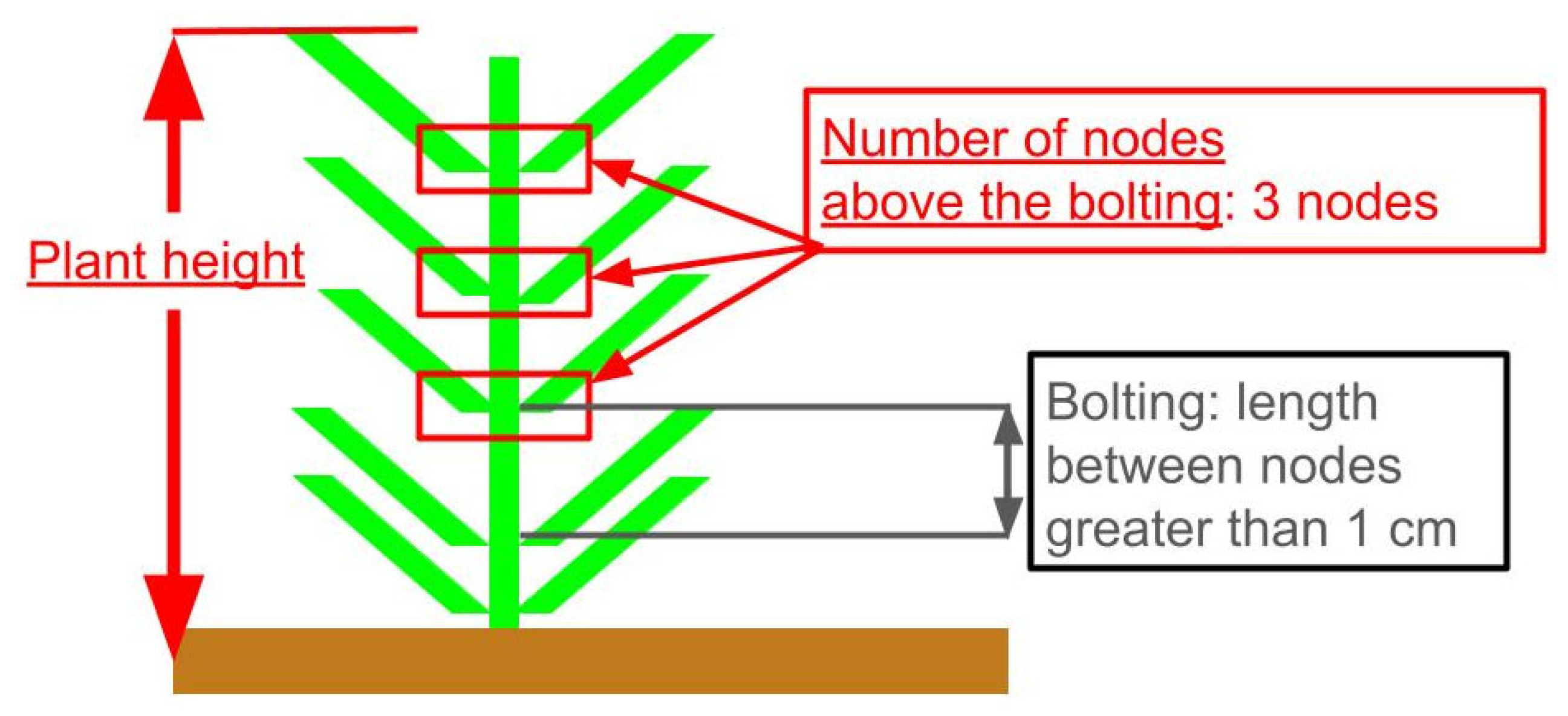
Figure 1. Diagram of the definition of plant height and the number of nodes above the bolting. The green part represents the plant body, and the brown part represents the ground.
Eng 06 00232 g001
Figure 2. Flowchart of plant height estimation.
Eng 06 00232 g002
Figure 3. Flowchart of the estimation of the number of nodes above the bolting.
Eng 06 00232 g003
Figure 5. Semantic segmentation results of point clouds at different growth stages. (ac) Original point clouds at early, middle, and late stages, respectively; (df) Corresponding segmentation results using RANSAC, where red indicates stem regions and blue represents leaf regions.
Eng 06 00232 g005
Table 2. Quantitative result of semantic segmentation by RANSAC.
IoUmIoUAcc
LeafStem
Early0.9330.4350.6840.937
Middle0.9240.6160.7700.932
Late0.9540.6940.8240.958
Average0.9370.5810.7590.942
Disclaimer/Publisher’s Note: The statements, opinions and data contained in all publications are solely those of the individual author(s) and contributor(s) and not of MDPI and/or the editor(s). MDPI and/or the editor(s) disclaim responsibility for any injury to people or property resulting from any ideas, methods, instructions or products referred to in the content.