Article

A Modular Framework for RGB Image Processing and Real-Time Neural Inference: A Case Study in Microalgae Culture Monitoring

by
José Javier Gutiérrez-Ramírez
1,
Ricardo Enrique Macias-Jamaica
2,
Víctor Manuel Zamudio-Rodríguez
1,
Héctor Arellano Sotelo
1,
Dulce Aurora Velázquez-Vázquez
3,
Juan de Anda-Suárez
4 and
David Asael Gutiérrez-Hernández
1,*
1
División de Estudios de Posgrado e Investigación, Tecnológico Nacional de México/IT de León, León 37290, Gto, Mexico
2
Departamento de Ingeniería Química, Tecnológico Nacional de México en Celaya, Celaya 38010, Gto, Mexico
3
Facultad de Arquitectura, Universidad La Salle Bajío, Av. Universidad 602. Col. Lomas del Campestre, León 37150, Gto, Mexico
4
Departamento de Ingeniería Mecatrónica, Tecnológico Nacional de México/ITS de Purísima del Rincón, Purísima del Rincón 36400, Mexico
*
Author to whom correspondence should be addressed.
Eng 2025, 6(9), 221; https://doi.org/10.3390/eng6090221
Submission received: 1 July 2025 / Revised: 15 August 2025 / Accepted: 22 August 2025 / Published: 2 September 2025
(This article belongs to the Special Issue Artificial Intelligence for Engineering Applications, 2nd Edition)

Abstract

Recent progress in computer vision and embedded systems has facilitated real-time monitoring of bioprocesses; however, lightweight and scalable solutions for resource-constrained settings remain limited. This work presents a modular framework for monitoring Chlorella vulgaris growth by integrating RGB image processing with multimodal sensor fusion. The system incorporates a Logitech C920 camera and low-cost pH and temperature sensors within a compact photobioreactor. It extracts RGB channel statistics, luminance, and environmental data to generate a 10-dimensional feature vector. A feedforward artificial neural network (ANN) with ReLU activations, dropout layers, and SMOTE-based data balancing was trained to classify growth phases: lag, exponential, and stationary. The optimized model, quantized to 8 bits, was deployed on an ESP32 microcontroller, achieving 98.62% accuracy with 4.8 ms inference time and a 13.48 kB memory footprint. Robustness analysis confirmed tolerance to geometric transformations, though variable lighting reduced performance. Principal component analysis (PCA) retained 95% variance, supporting the discriminative power of the features. The proposed system outperformed previous vision-only methods, demonstrating the advantages of multimodal fusion for early detection. Limitations include sensitivity to lighting and validation limited to a single species. Future directions include incorporating active lighting control and extending the model to multi-species classification for broader applicability.

1. Introduction

Over the past decade, computer vision has evolved from classic digital image processing into an indispensable component of embedded systems, where computational efficiency, modular design, and autonomous operation are mandatory for sectors as diverse as biomedicine, protected agriculture, and mobile robotics [1,2,3]. This progress has been driven by hardware innovations such as pixel-parallel processor arrays (PPAs) and domain-specific architectures (DSAs) that deliver low latency and high energy efficiency for real-time, compute-intensive machine-learning tasks [4,5]. In parallel, algorithmic advances, particularly evolutionary computer vision, have enabled the solution of complex problems through stochastic and metaheuristic optimization, maximizing resource use in constrained environments [6]. Evolutionary neural networks now achieve outstanding accuracy in classification and segmentation, and frameworks such as CNNParted show how model partitioning and quantization can balance accuracy and power draw on low-cost devices [7]. Nevertheless, designing truly generic architectures that seamlessly combine these hardware-software advances while ensuring portability and scalability amid the rapid emergence of new models remains an open challenge [8].
To validate the modular framework proposed in this study, we applied it to the monitoring of Chlorella vulgaris cultures. Fusing RGB images of cell density with multimodal data on pH and temperature enables continuous, non-invasive tracking of growth kinetics in Chlorella vulgaris, where each phase exhibits unique biochemical signatures that align with our RGBI features. During the lag phase, cells prioritize adaptation through enzyme synthesis and chlorophyll production (primary metabolites), detectable as gradual increases in green-channel intensity (G). The exponential phase (critical for biofuel applications due to rapid accumulation of lipids and proteins) shows strong correlations with sharp rises in luminance (I) and chromatic variance. As nutrients deplete in the stationary phase, cells shift to storage compounds (e.g., starch) and secondary metabolites like carotenoids marked by stabilized RGB means and increased dispersion from cell aggregation. This biochemical-photometric linkage, enhanced by pH/temperature data (e.g., detecting acidification during lipid turnover), provides a robust framework for strain selection and process optimization, particularly for high-value metabolites [9,10,11]. Low-cost devices for biomass quantification have also been developed for resource-limited settings [10]. Real-time models based on YOLO and R-CNN variants report mean average precision (mAP) above 0.95 for microalgal cell detection in micrographs, confirming feasibility on computationally constrained embedded platforms [12,13,14]. A MobileNet + Spatial Pyramid Pooling variant of YOLOv3 achieved 98.90% accuracy on ballast-water samples, underscoring the effectiveness of lightweight architectures [15,16]. Advanced systems such as the Confocal Hyperspectral Microscopic Imager (CHMI) have reached 98.34% identification rates with deep networks, improving phenotypic resolution without complex sample preparation [17]. Traditional optical methods based on absorption and scattering remain essential for assessing biomass and stress responses, and their integration with machine-learning algorithms could yield more robust, scalable monitoring [18]. For a comprehensive edge-oriented characterization, future studies should report inference latency and energy consumption.
Although many optimized YOLOv5 versions have been proposed for edge deployments, they typically target narrow tasks and lack cross-platform evaluations of latency, power, and accuracy. For instance, ref. [19] introduced SCB-YOLOv5, replacing the backbone with ShuffleNetV2 and adding a BCS-FPN attention module, reducing parameters by 22.4% and FLOPs by 21.7% for traffic-sign detection, yet omitting inference-time and power metrics on embedded hardware. The authors of ref. [20] developed a GSConv-enhanced YOLOv5 for PCB defect detection, achieving 94.9% mAP@0.5 with 53.7% fewer parameters but without scalability tests across domains. Surveys of pruning, quantization, and knowledge distillation still report no latency-or-energy data on low-cost devices [21,22]. Ref. [23] showed that YOLOv5 (35.6 FPS, 3.2 GB GPU) and Swin Transformer (3.9 FPS, 12.2 GB) reach 90–95% accuracy under controlled conditions, but their reliance on costly hardware and sensitivity to misalignment (performance drops to 94% under calibration errors) hinder scalability. The authors of ref. [24] reported 98.8% mAP and 41 ms inference on FPGA for railway-component detection, yet their design is domain-specific, hardware-intensive, and lacks multimodal adaptability. The authors of ref. [25] presented LFD-YOLO, integrating GhostConv and an Efficient Multi-Scale Attention block, improving mAP@IoU = 0.5–0.95 by 0.5 pp and cutting FLOPs by 35%, but without energy or portability benchmarks on diverse embedded platforms. The authors of ref. [26] showed that structured pruning and full-integer quantization can save up to 40% energy on sensor-edge systems, yet they did not test cross-domain accuracy. The authors of ref. [27] applied dynamic sparse learning for aerial tracking to lower inference latency by 30%, but energy use and scalability on heterogeneous hardware remained unreported. Previous work achieved 9 ms sampling and 90.2% accuracy in structured industrial settings [28,29] and 91.5% AP for open-field strawberry harvesting [30], yet lacked FPS data and multiscale tests. These gaps highlight the need for a unified framework that merges multimodal RGB + environmental capture with a lightweight, SMOTE balanced ANN and delivers thorough assessments of inference latency, power draw, and accuracy across growth stages.
In this paper, we present a modular embedded monitoring framework that acquires real-time RGB images of a region of interest (ROI) together with pH, temperature, and light-intensity readings to classify the growth phases of Chlorella vulgaris. We design a sequential multilayer artificial neural network (ANN) for three-class prediction (lag, exponential, stationary) using ReLU activations to mitigate vanishing gradients, dropout layers (0.2–0.5) to prevent overfitting, and categorical cross-entropy optimized with Adam (learning rate = 0.001); growth-phase labels are one-hot encoded. The output layer uses softmax activation to normalize predictions into a probability distribution across the three phases (Lag, Exponential, Stationary). Sparse categorical cross-entropy was chosen as the loss function because it directly penalizes misclassifications in one-hot encoded labels, synergizing with SMOTE to improve minority-class recall [31]. This combination is ideal for imbalanced biological data where phase transitions are critical. The system is deployed in a low-cost smart photobioreactor, where it achieves 0.995 ± 0.001 accuracy (validated by 40 k-fold runs), 50 ms inference latency, and modest resource usage. Principal component analysis (PCA) confirms class separability while retaining 95% of the original variance. These results demonstrate the framework’s scalability for edge-computing scenarios and its potential transfer to other computer-vision domains under resource constraints.

2. Materials and Methods

2.1. Experimental System

Experiments were run in triplicate to increase data reliability and to build a robust, structured data set for multimodal learning. A purposembuilt cylindrical smart photobioreactor (working volume = 4 L, 10 cm inner diameter, 50 cm height) was assembled from PVC tubing and 3D printed mounts, facilitating direct integration of sensors and imaging devices [32]. Airflow was regulated by a needle valve (1.5–2.5 L min−1), while constant illumination was provided by twelve cool-white LEDs (≈ 6000 K, 400–700 nm) driven by PWM from an ESP32 microcontroller. A PH-4502C pH electrode and a DS18B20 temperature probe were installed 15 cm above the base; a Logitech C920 HD camera (3 MP) was fixed 10 cm from the reactor wall, capturing a centered 250 × 250-px region of interest (ROI).
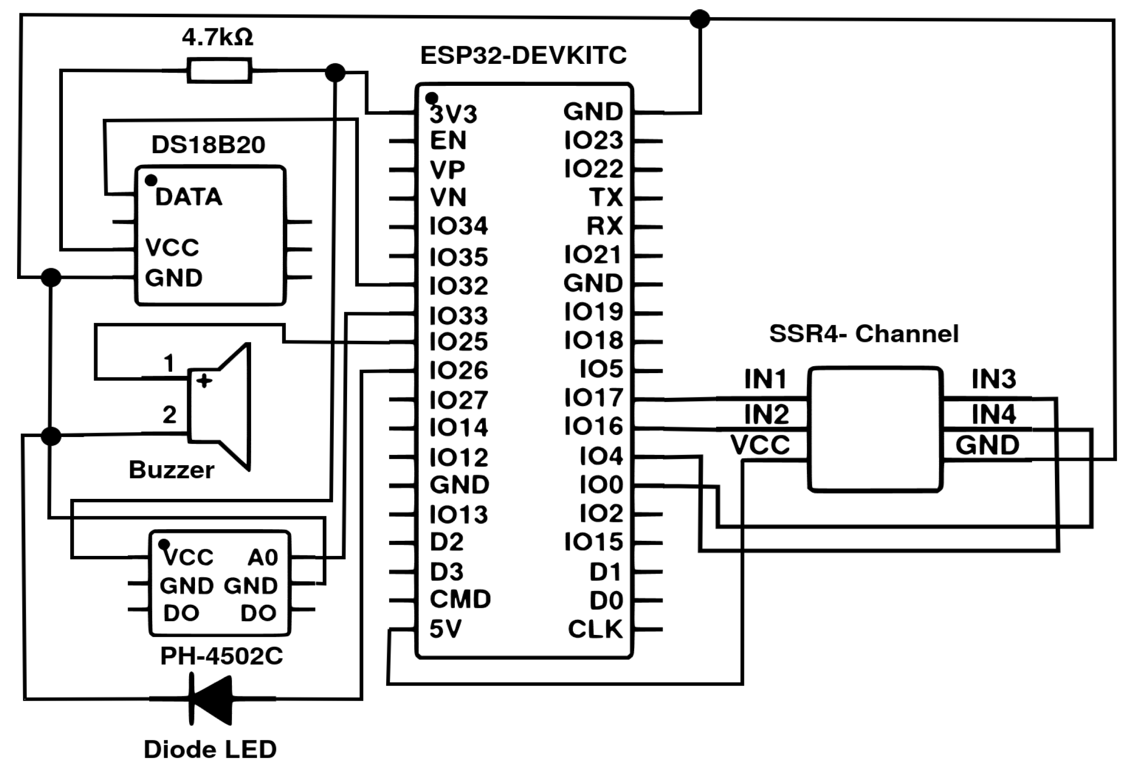
While optical methods such as fluorescence-based pH measurement offer high precision, this study prioritizes computational feasibility and cost-effectiveness for resource-constrained environments. The PH-4502C electrode was selected due to its compatibility with embedded systems and minimal calibration requirements, despite potential trade-offs in resolution compared to advanced biochemical techniques. The framework’s core innovation lies in fusing RGB image features with low-cost sensor data, rather than relying on specialized instrumentation. Future iterations could explore hybrid optical–computational approaches if budgetary and technical constraints are alleviated. Images were acquired hourly during three non-overlapping cultivation cycles (12 February–7 March, 12 March–11 April and 11 April–23 May 2025) totaling 98 days. Unequal cycle lengths are inconsequential, as the goal is not to compare yields but to supply diverse data for multimodal training. Figure 1 shows the 3D layout with sensor and camera positions; Figure 2 details the ESP32 wiring diagram.
All cultivation cycles used the same strain of Chlorella vulgaris, obtained commercially and scaled to an initial volume of 900 mL (1:3 inoculum-to-water ratio) using potable water and an unspecified nutrient supplement (blue powder formulation). The culture medium was maintained at 25–28 °C, with aeration provided by an aquarium pump (2.0 L min−1) via a needle valve, ensuring consistent dissolved oxygen levels. Illumination was supplied by a 6W white LED panel (≈6000 K, 400–700 nm) positioned beneath the reactor, with photoperiods aligned to natural growth phases. The system was sealed with a 3D-printed lid and covered with a black fabric to minimize external light interference, the LED panel provided consistent bottom-up illumination (6W, 6000 K), ensuring that luminance (I) measurements directly correlated with microalgal density. As cells grew, light transmission decreased due to chlorophyll absorption, enabling phase detection without background subtraction. This design intentionally avoids ‘light-off’ scenarios, as the proposed method relies on dynamic light attenuation by the culture itself. pH remained stable (7.20–10.40) across cycles, though nutrient depletion in stationary phases likely influenced metabolic byproducts. Notably, lag phases varied significantly (0.1–113.4 h), attributed to initial adaptation in later cycles, while exponential (5.1 days avg) and stationary phases (23.9 days avg) showed consistent durations. Failures occurred only under power interruptions, highlighting the system’s dependence on stable electricity despite its low-cost design.
The proposed system relies on non-invasive RGB image analysis as a proxy for biomass density, avoiding destructive sampling or expensive laboratory equipment (e.g., spectrophotometers). While traditional methods like optical density (OD680) or dry weight measurements provide absolute biomass quantification, this study prioritizes a low-cost, vision-based proxy for phase classification. The RGBI features (e.g., luminance II) correlate with growth phases through kinetic patterns (Section 3.1.1), eliminating the need for laboratory-grade calibration. This approach aligns with prior works in microalgae monitoring [33,34], where relative color shifts (not absolute biomass), are sufficient for phase discrimination in resource-constrained settings.

2.2. Framework Architecture

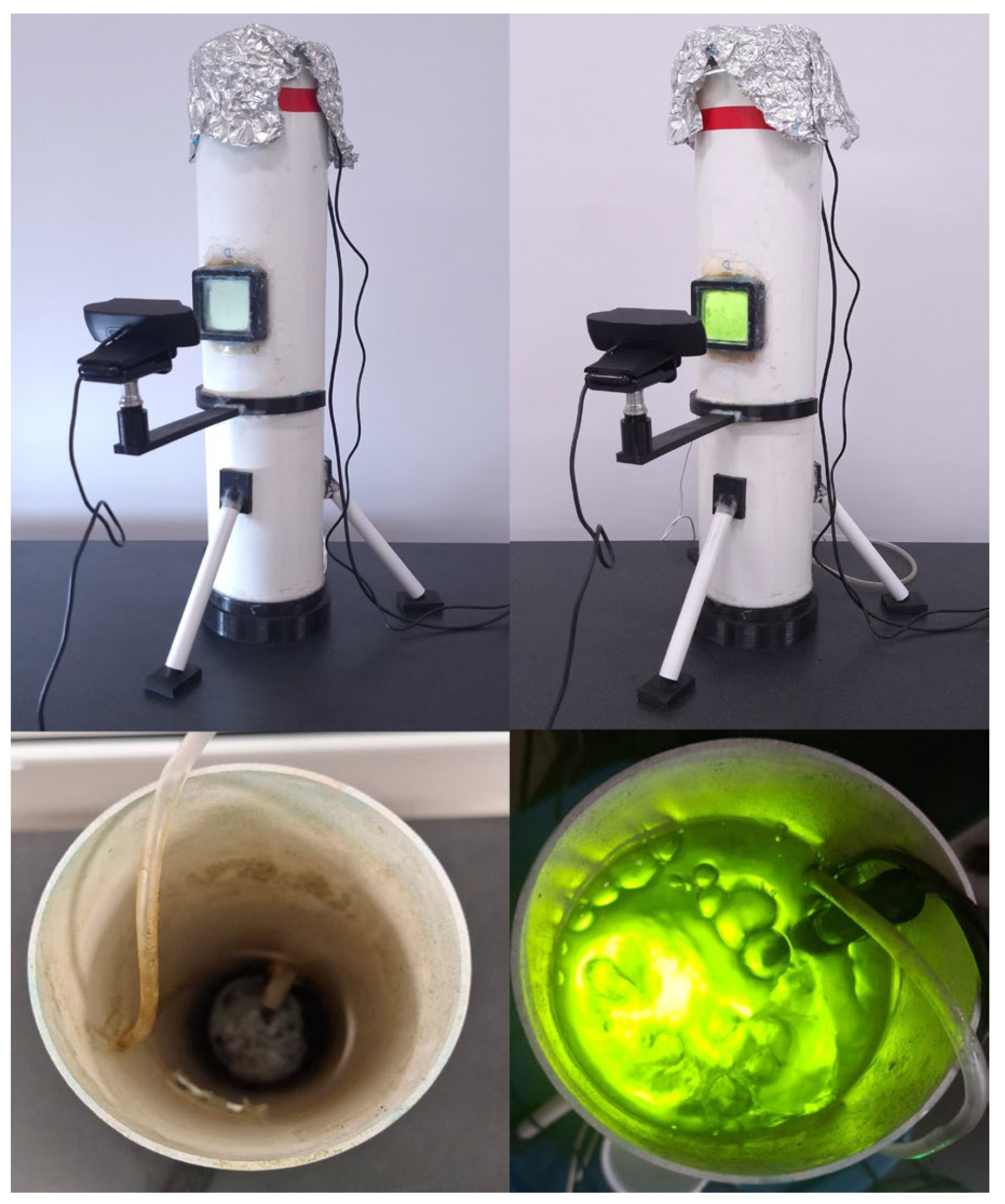
Figure 3 summarizes the four-stage workflow. (i) Image capture: RGB frames are acquired under fixed white balance, exposure, and focus. (ii) Multimodal fusion: the ROI is cropped, channel statistics are extracted, and concatenated with synchronous pH and temperature readings to form a feature vector. (iii) Prediction: a pre-trained artificial neural network (ANN) classifies the culture as lag, exponential, or stationary. (iv) Adaptive control: the ESP32 adjusts LED intensity, aeration rate, or temperature according to the predicted phase, closing an intelligent feedback loop. The physical setup used for image acquisition and environmental control is shown in Figure 4, which depicts the photobioreactor prototype used.

2.3. Data Acquisition and Preprocessing

The Logitech C920 operated at its native 3 MP resolution; autofocus was disabled (cv2.CAP_PROP_AUTOFOCUS = 0, value 65) as was auto-exposure (cv2.CAP_PROP_AUTO_EXPOSURE = 0.1, value 60). The camera mount ensured spatial repeatability. Background subtraction was unnecessary due to the fixed camera alignment and ROI cropping (250 × 250 px center region). The reactor’s sealed design and controlled illumination (cool-white LEDs at 6000 K) ensured consistent imaging conditions, with the ROI containing only the culture medium. Autofocus and auto-exposure were disabled (cv2.CAP_PROP_AUTOFOCUS = 0, cv2.CAP_PROP_AUTO_EXPOSURE = 0.1) to prevent artifacts from ambient light changes. This setup inherently isolates the culture from background interference, as validated by the model’s tolerance to geometric perturbations (Section 3.4).
The system captures a dynamic range of cell densities corresponding to all growth phases (Lag, Exponential, Stationary), as evidenced by the luminance values (1.8–251.2 in 8-bit scale, Table 1). While absolute density quantification was beyond this study’s scope, the framework’s robustness across phases (Section 3.1) confirms its suitability for low-to-medium density cultures typical of lab-scale photobioreactors.

2.4. Multimodal Feature Construction

Each sample is encoded as a ten-element vector:
[ R ¯ ,   G ¯ ,   B ¯ ,   I ¯ ,   σ R ,   σ G ,   σ B ,   σ I ,   p H mean ,   T mean ]
For pHmean and Tmean, twenty readings spaced 2 s apart were filtered for outliers with the IQR method and averaged. The ROI was converted from BGR to RGB, smoothed with a 5 × 5 Gaussian kernel, and per-channel means and standard deviations were computed. Perceptual luminance ( I ¯ ) was computed using the Rec. 709 standard formula: I = 0.2126 R + 0.7152 G + 0.0722 B [ITU-R BT.709−6, 2015]. This weighting reflects both human vision sensitivity (green > red > blue) and Chlorella vulgaris’ spectral response, where chlorophyll-a absorbs predominantly in red/blue wavelengths (400–500 nm, 600–700 nm), making green channel intensity (500–600 nm) a robust proxy for biomass density [9,10]. The formula thus aligns optical measurements with both physiological relevance and computational efficiency, the standard deviation is σI. Table 1 lists observed ranges and normalization parameters.
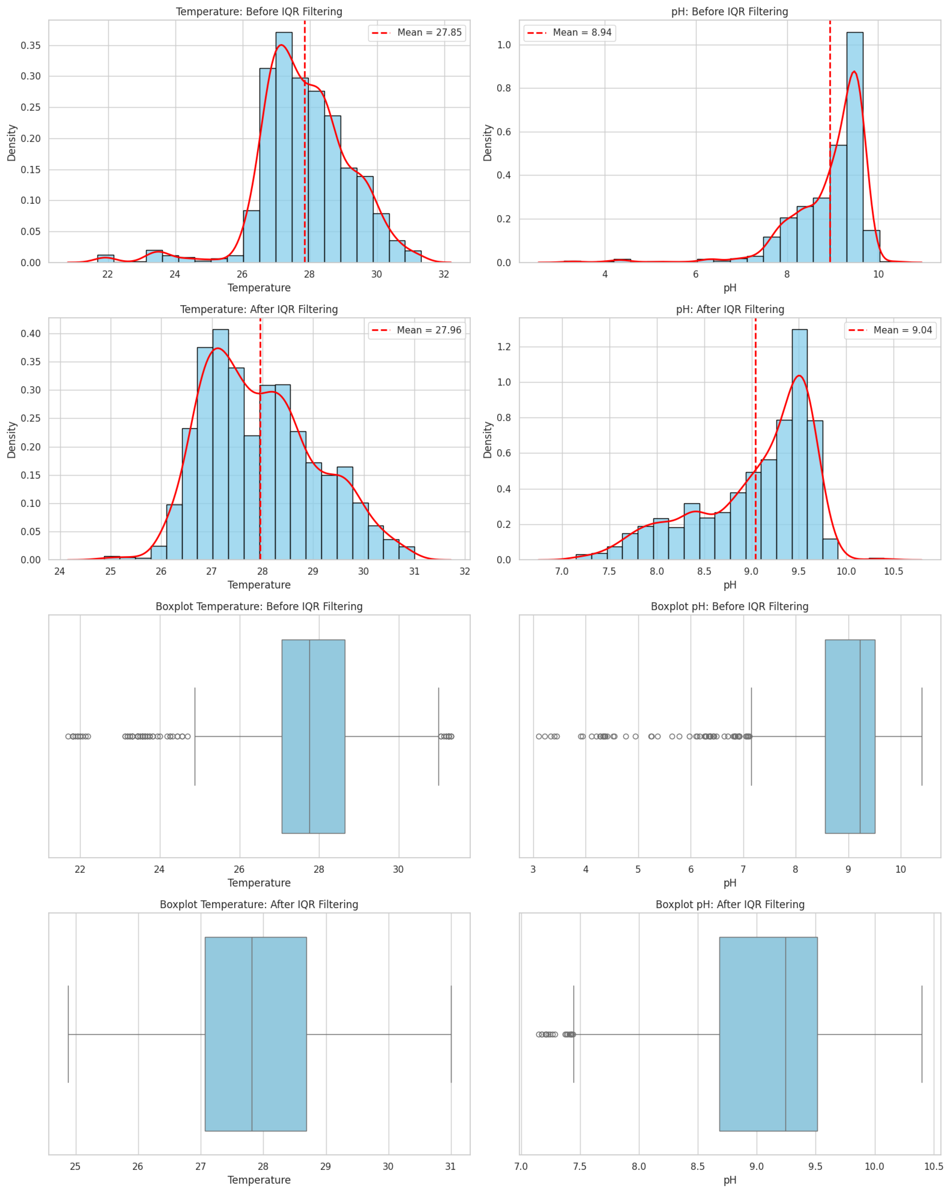
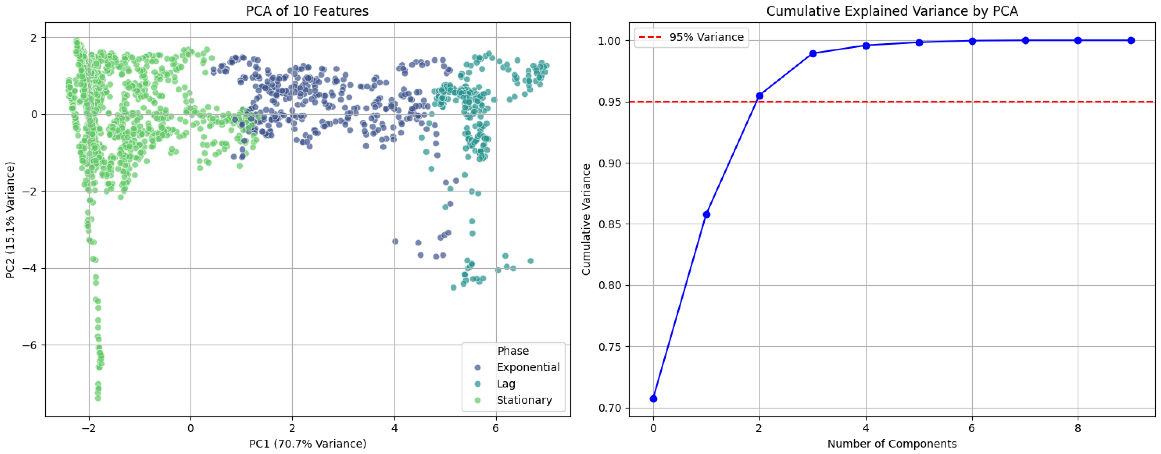
Outliers in pH and temperature were filtered using the IQR method (threshold: 1.5 × IQR). Shapiro–Wilk tests confirmed non-normality in raw data (p < 0.001), but Z-score normalization (Table 1) mitigates skewness. Histograms and boxplots (Figure 5) show that removed outliers were extreme values (e.g., sensor noise during aeration), not biological trends: mean pH/temperature shifted minimally (8.93→9.03, 27.85→27.95 °C). PCA (Figure 6) retained 95% variance after filtering, confirming that critical phase-discriminative features were preserved. This aligns with studies showing that microalgae growth kinetics are robust to minor sensor fluctuations [9,10].

2.5. Neural Network Training

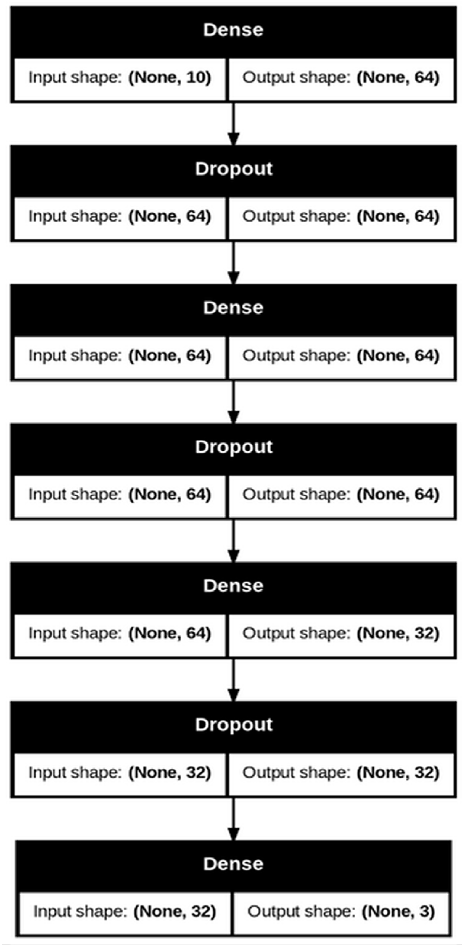
The classifier is a feedback RNA implemented in Keras, designed to optimize efficiency and deployment on hardware with limited resources. While the architecture is not novel, its optimization (quantization, dropout, and SMOTE balancing) addresses deficiencies in previous work by combining low latency (<5 ms) with high accuracy (98.6%) in embedded systems, a balance rarely achieved in microalgae monitoring. The 10-unit input layer feeds into three dense layers of 64, 64, and 32 neurons with ReLU activations (Figure 7), and the final layer uses a SOFTMAX activation function. Each hidden layer has a dropout rate of 0.2 to 0.4, and early stopping (patience = 5) restores the best weights. Adam optimization uses a learning rate of 0.001 and sparse categorical cross-entropy loss (sparse_categorical_crossentropy). Class imbalance is mitigated with SMOTE [35]. Five-fold cross-validation, repeated 40 times with different seeds, provides accuracy, recall, F1 score, and AUC-ROC. Data partitioning followed a stratified 5-fold cross-validation scheme (repeated 40× with random seeds) to ensure balanced representation of all growth phases in training/validation sets. Each fold used 80% of data for training and 20% for validation, iterating until all subsets were evaluated. This rigorous approach mitigates overfitting and provides robust performance metrics (Section 3.1).
Categorical cross-entropy was chosen over alternatives (e.g., MSE) because it directly optimizes probabilistic confidence in mutually exclusive growth phases (Lag = 0, Exponential = 1, Stationary = 2), penalizing misclassifications more sharply when probabilities diverge from one-hot encoded labels [31]. This aligns with SMOTE-augmented data, as the loss function’s gradient updates prioritize correcting errors in minority classes (e.g., exponential phase), synergizing with synthetic samples to improve recall (Table 2). The combination of SMOTE and categorical cross-entropy ensured balanced learning across phases despite their inherent biochemical asymmetry (e.g., longer stationary phases in fermentation).
The dataset exhibited an inherent class imbalance (Figure 8), with the stationary phase representing 70.8% of the samples, while the exponential and lag phases accounted for 18.1% and 11.1%, respectively, a distribution consistent with microbial growth kinetics, where the stationary phase tends to dominate cultivation timelines [9]. To ensure robust learning across all phases, SMOTE [35] was applied to synthetically balance the minority classes (Lag and Exponential) by generating interpolated samples within their feature-space neighborhoods. This approach preserved the physiological relationships encoded in the original 10-dimensional vectors (RGBI, pH, temperature), as evidenced by the model’s high recall (>99% for all phases) and macro F1-score (98.94%). The near-perfect AUC-ROC (0.9999) further confirms that SMOTE-enhanced training did not introduce artifactual separability between classes.

2.6. Implementation and Computing Environment

All software is written in Python 3.13.5. OpenCV handled image processing; NumPy supported numerical routines; PyMySQL logged data to MySQL; FastAPI exposed a REST endpoint; APScheduler triggered hourly tasks. The back-end server (Ubuntu, Intel i3 7th Gen, 4 GB RAM) receives data from an ESP32 (firmware in C++ using OneWire, DallasTemperature, ArduinoJson). The trained model was converted to TensorFlow Lite for Microcontrollers with 8-bit post-training quantization, shrinking it to 13.48 kB and providing 4.8 ms inference on the ESP32 (≈512 kB SRAM).
The trained model was optimized for embedded deployment using TensorFlow Lite for Microcontrollers with 8-bit post-training quantization. This process reduced the model size by 4× (from 54 kB to 13.48 kB) by converting floating-point weights to integers, while maintaining >98% accuracy through calibration with representative data. Key deployment metrics included inference latency (4.8 ms, measured via ESP32 cycle counters), memory footprint (<25 kB RAM, verified via TensorFlow Micro’s memory arena allocator), and CPU utilization (24% at 50 inferences/s). The quantization-aware training (QAT) strategy minimized precision loss by preserving critical weight distributions for RGBI and sensor features, ensuring robust phase classification despite integer-only arithmetic. These metrics were validated against the original FP32 model using a holdout test set, confirming <2% deviation in F1-score.

2.7. Robustness Validation

Robustness was evaluated on 50 representative images. Controlled perturbations included ROI shift (+10 px), brightness increase (+50 levels), Gaussian noise (σ = 25), rotation (+15°), zoom (±10%), Gaussian blur (5 × 5) and partial occlusion (25%). Shifts and rotations changed means by <8% and standard deviations by <20%. Increased brightness raised channel means proportionally; noise tripled standard deviations while leaving means virtually unchanged. Zoom-in reduced dispersion up to 40%, whereas zoom-out increased it up to 50%. Blur lowered standard deviations by 10–15%. Occlusion decreased means by up to 20% and inflated dispersion by 150%. The system remained stable under minor geometric perturbations but was sensitive to lighting changes and occlusions, confirming that RGBI means are reliable growth indicators provided illumination is controlled and the ROI remains unobstructed.

3. Results

3.1. Overall Classification Performance

The multimodal classifier achieved outstanding performance when distinguishing the growth phases of Chlorella vulgaris (Lag, Exponential and Stationary) from RGBI descriptors, channel wise standard deviations and physicochemical variables (pH, temperature). Averaging 40 independent runs with 5-fold stratified cross validation yielded a macro accuracy of 98.62%, Recall of 99.29%, F1-score of 98.94% and an AUC-ROC of 0.9999 (Table 2). Stationary achieved the highest classwise Accuracy (99.97%), followed by Lag (99.24%) and Exponential (96.66%). Exponential obtained the highest Recall (99.41%), showing that the model captures early-growth patterns even under subtle variations in cell density. The near-perfect separability (AUC-ROC ≈ 1) confirms that the multimodal vector faithfully reflects the physiological dynamics of each stage, providing a reliable basis for automated photobioreactor monitoring.
From a bioprocess perspective, these metrics translate directly to culture management: Loss (0.02 ± 0.01) quantifies the model’s error in predicting phase transitions critical for timing nutrient feeds or harvesting. Accuracy (98.6%) ensures reliable phase identification (e.g., avoiding premature induction during lag). Recall (99.3%) guarantees minimal missed exponential phases where metabolite production peaks, while F1-score balances false positives/negatives that could disrupt batch scheduling. The near-perfect AUC-ROC (0.9999) indicates robustness against noise inherent in bioreactor environments (e.g., bubbles, sensor drift), outperforming traditional OD600 measurements that often conflate lag and early exponential phases [9,10].
Growth phase labeling was performed through a hybrid approach combining unsupervised clustering and kinetic validation. First, phases were classified via k-means clustering (k = 3) of standardized RGBI and pH features, where centroids ordered by mean RGBI intensity assigned lag (highest I), exponential, and stationary phases (lowest I). This phenotypic grouping was then validated by calculating specific growth rates (μ = Δln(I)/Δt), yielding biologically plausible μ_max values (0.04–0.14 h−1) that align with reported ranges for C. vulgaris under similar conditions [36]. The clustering successfully captured phase transitions, with exponential-phase μ_max values correlating to centroid-derived classifications. While k-means provided initial phase boundaries, growth rates confirmed kinetic consistency, particularly in distinguishing late-exponential and stationary phases where RGBI plateaus. This dual methodology addresses limitations of purely unsupervised approaches by integrating both phenotypic (color) and dynamic (μ) criteria, as demonstrated in similar microbiological studies [37].

3.1.1. Growth Kinetics Analysis

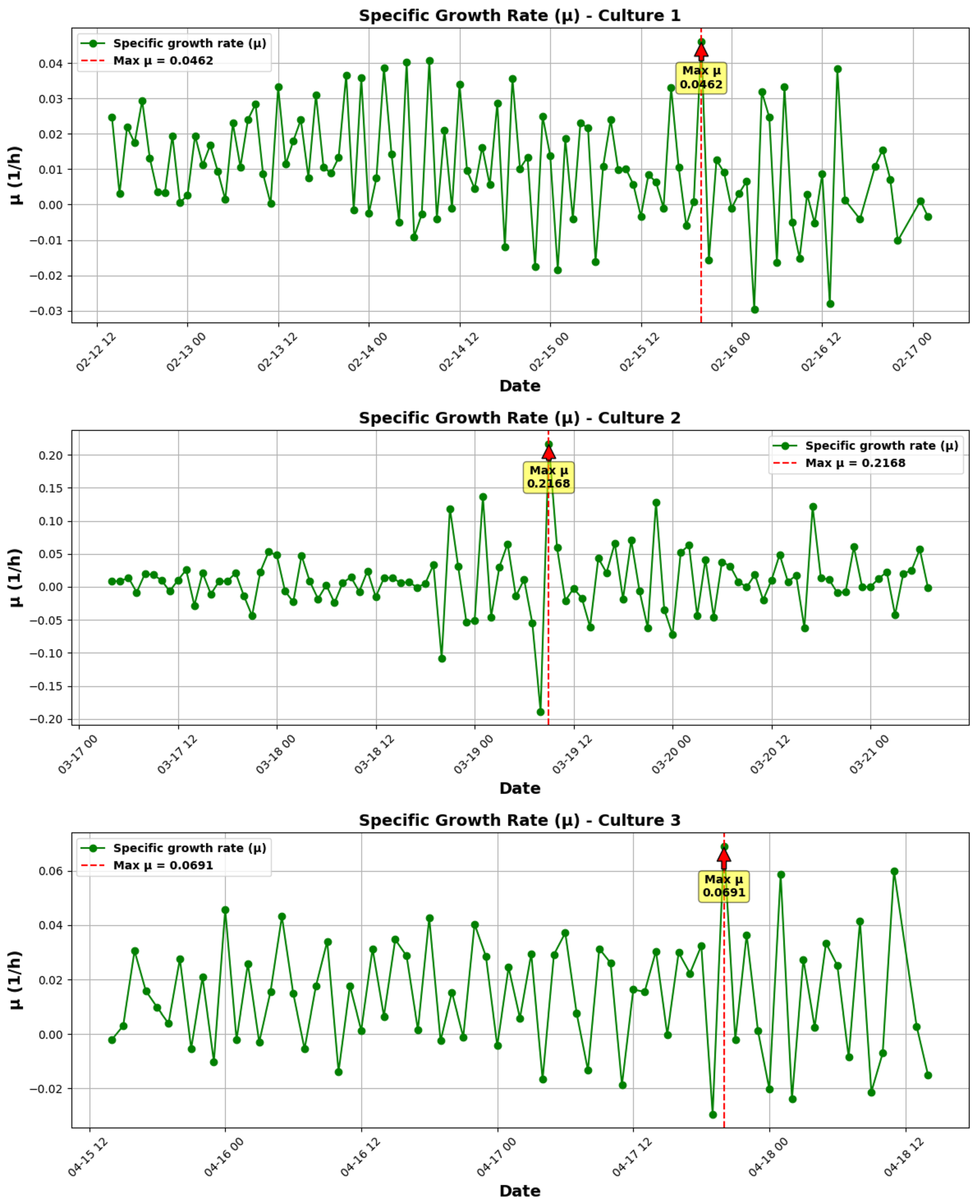
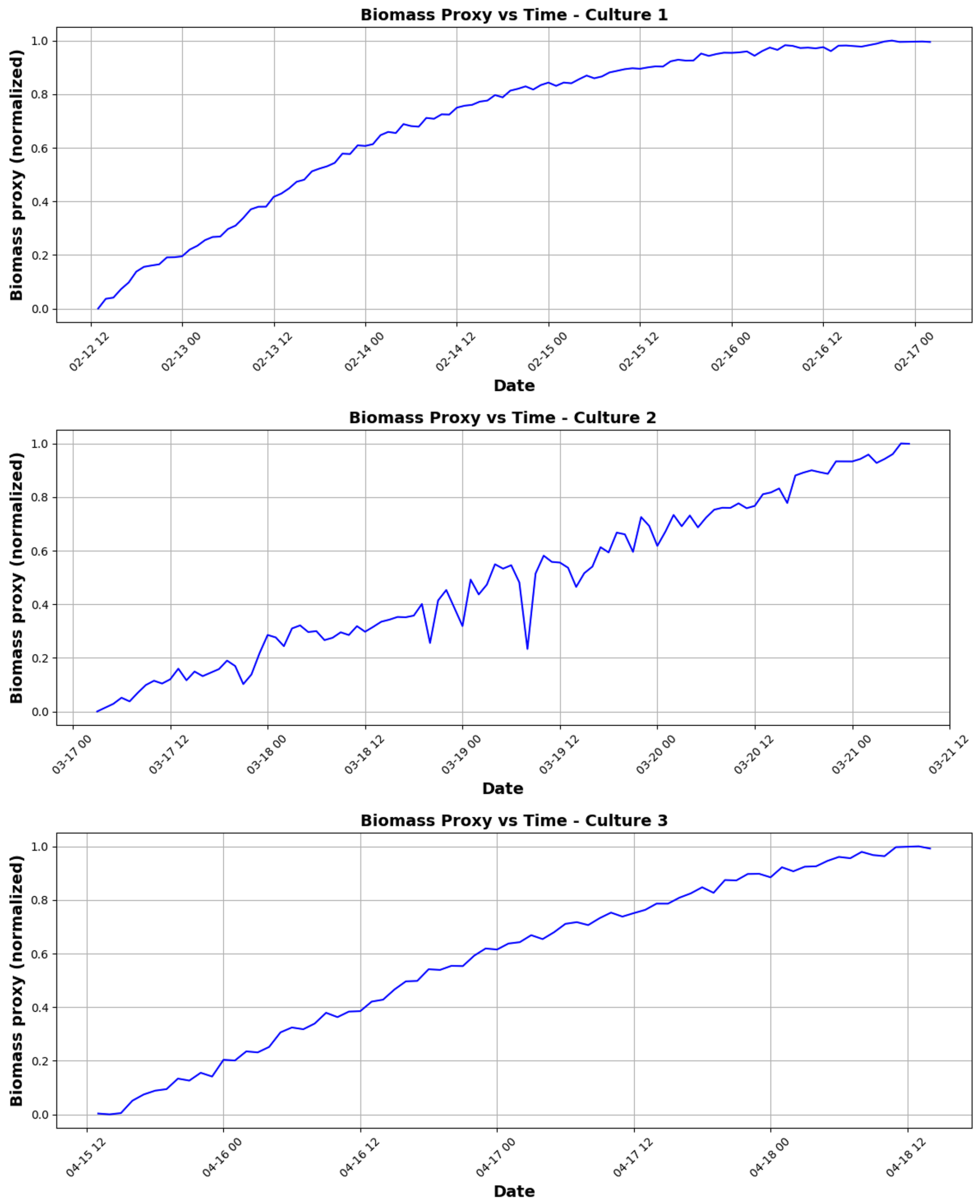
The specific growth rates (μ) during exponential phase were calculated from luminance (I) using the relationship μ = Δ(ln(I))/Δt (Figure 9), yielding μ_max values of 0.0407 h−1 (Culture 1), 0.1365 h−1 (Culture 2), and 0.0691 h−1 (Culture 3). These variations reflect differences in environmental conditions (e.g., temperature fluctuations of 25–29 °C and pH 7.8–9.6), consistent with reported μ ranges for Chlorella vulgaris under similar settings [33]. The biomass proxy (normalized I) showed classical growth kinetics (Figure 10), with Culture 2 exhibiting rapid early-phase growth (μ_max > 0.13 h−1) followed by decline, suggesting possible light/nutrient limitation. While direct cell counts were unavailable, the strong correlation between I and growth phases aligns with studies validating RGB-based biomass estimation in microalgae [33,34], where luminance reduction corresponds to increased cell density and chlorophyll content. Future work should incorporate offline OD680 measurements to refine this relationship. It is important to note that this study does not aim to fit kinetic models (e.g., Monod) due to the absence of substrate concentration data. Instead, the ANN classifies growth phases based on real-time RGBI trends and environmental sensors, a pragmatic solution for low-cost monitoring where traditional biochemical assays are unavailable. Future iterations could explore hybrid models if nutrient data becomes accessible. While Monod kinetics were not formally fitted due to substrate data unavailability, the μ_max variability aligns with Monod’s dependence on environmental factors. Future studies should integrate nutrient monitoring to enable such modeling.

3.2. Training Curves

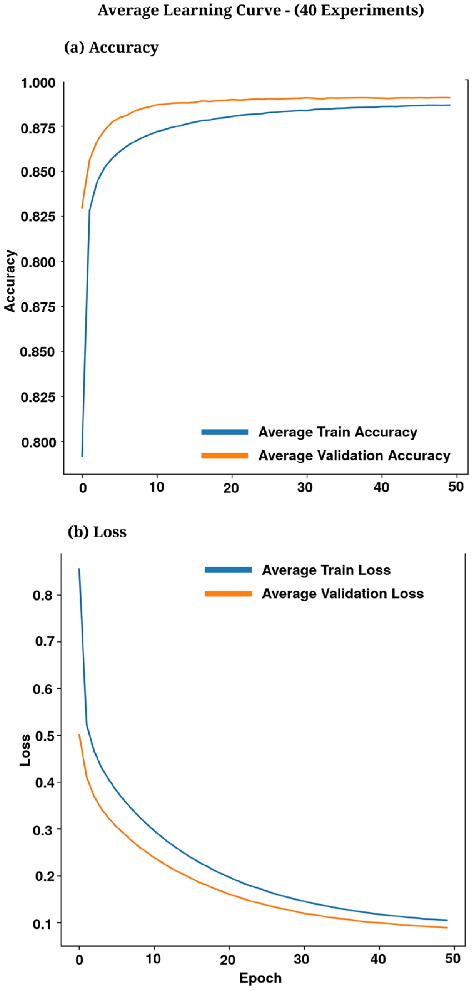
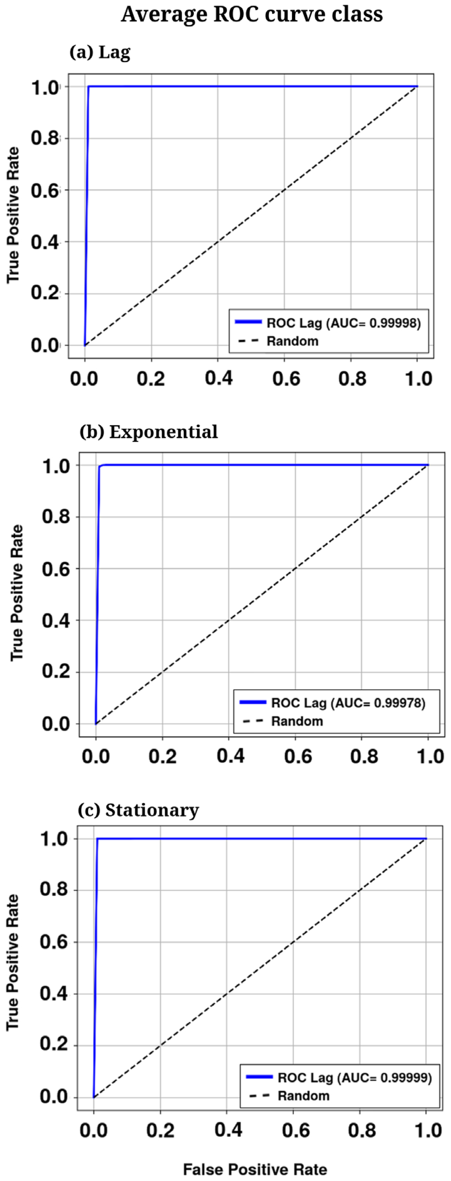
The average loss and Accuracy curves (Figure 11) exhibit stable convergence between the training and validation sets, with no evidence of overfitting. On average, Early Stopping triggered at epoch 46, reaching 99.23% validation Accuracy with a minimum validation loss of 0.02 ± 0.01. The gap between training and validation remained below 0.5% in Accuracy and 0.01 in loss, confirming strong generalization. Final per-run metrics were consistent: Accuracy 99.21 ± 0.15%, Precision 99.21 ± 0.15%, Recall 99.22 ± 0.14%, F1 score 99.21 ± 0.14% and AUC-ROC 0.9998 ± 0.0001 (Figure 12).

3.3. Confusion Matrix Analysis

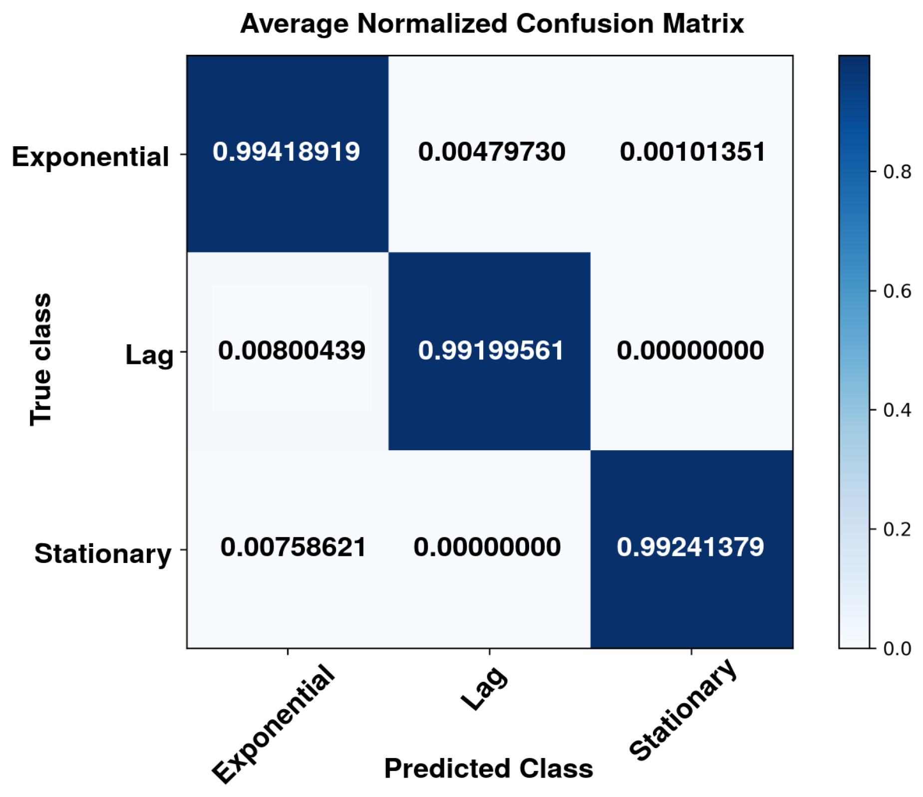
The normalized confusion matrix (Figure 13) shows diagonal values > 99%, indicating near-perfect classification. The few errors (<1%) occurred only between adjacent phases: exponential → lag (0.51% false positives) and lag → exponential (0.81%), attributable to gradual transitions in density and pigmentation. Stationary was never confused with Lag and only 0.76% with Exponential, demonstrating that the multimodal descriptors clearly separate extreme phases. With specificity > 99.2% and AUC-ROC ≥ 0.9998, the approach is well suited to control systems that require early alerts during the exponential phase, which is critical for culture optimization.

3.4. Robustness Evaluation

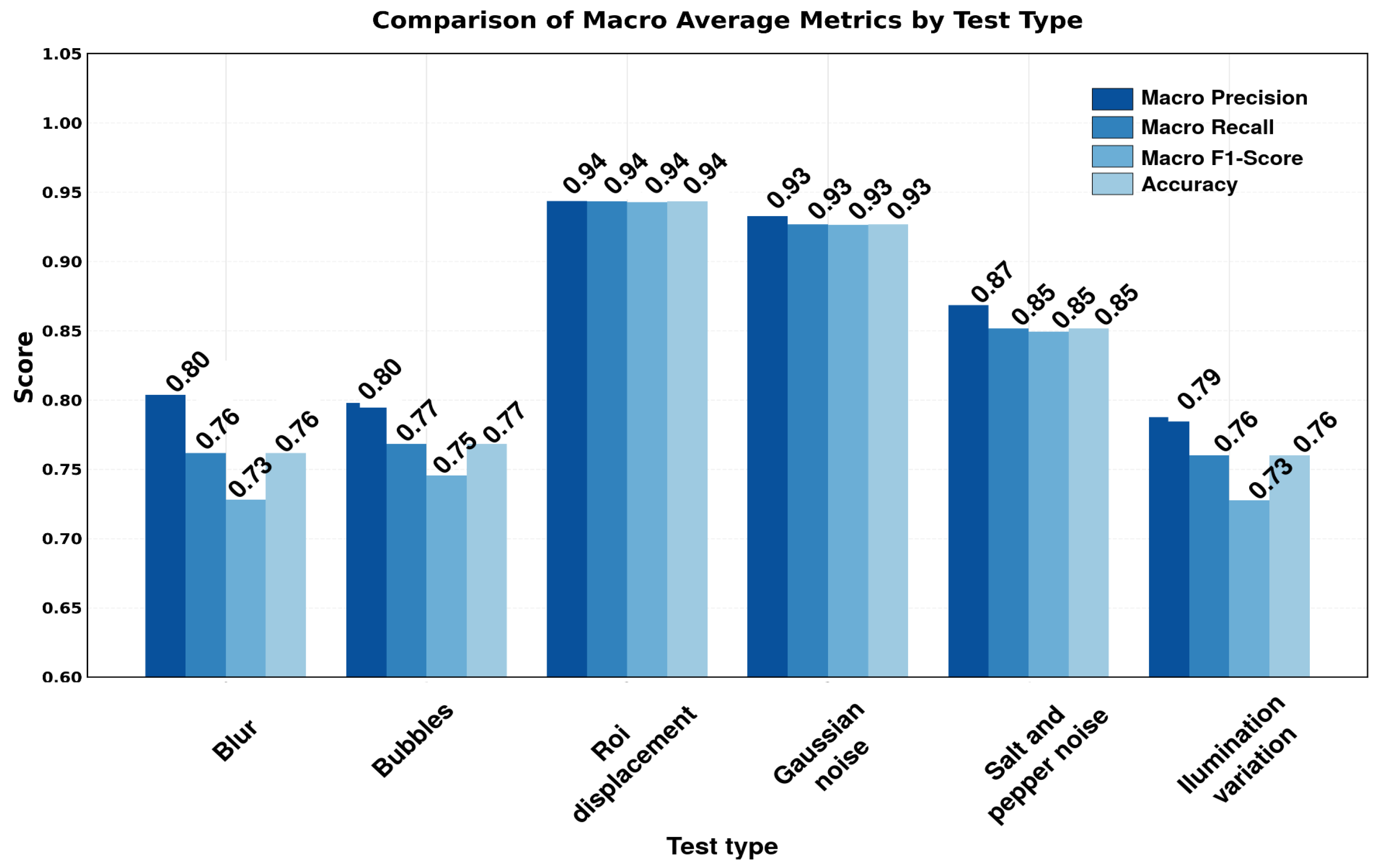
Figure 14 summarizes accuracy degradation under controlled perturbations. Variable illumination produced the largest drop, reducing macro accuracy to 76.0% (F1 = 0.728), although lag retained 100% recall. ROI shift (+10 px) and Gaussian noise (σ = 25) had minor effects (Accuracy 94.3% and 92.7%, respectively). Gaussian blur (5 × 5) and bubbles caused moderate declines (76–85% Accuracy), mainly affecting exponential (F1 0.53–0.88). These results highlight the need for stable lighting and unobstructed ROIs; nonetheless, the model maintains > 92% accuracy in most scenarios and shows strong resilience for lag and stationary.
Variable illumination produced the largest drop, reducing macro accuracy to 76.0% (F1 = 0.728). This aligns with prior studies: uncontrolled lighting alters RGBI features by (i) skewing pigment reflectance (e.g., chlorophyll absorbs red/blue light, but excessive green illumination saturates the G channel [17,18]), and (ii) introducing noise in luminance (I) due to non-linear cell responses to light stress [18]. For instance, Solovchenko [18] showed that high light intensity degrades chlorophyll (reducing R/B means) while triggering carotenoid production (inflating G). Our synthetic tests (brightness +50 levels) replicated this, causing misclassifications when exponential-phase cultures were misread as Lag due to G-channel saturation. Although our fixed LED setup minimized natural variability, the results underscore the need for active lighting control or spectral normalization (e.g., ExG index [16]) to stabilize features. Notably, lag phase retained 100% recall even under illumination shifts, suggesting pH/temperature sensors compensate for optical artifacts during early growth.

3.5. Computational Performance

On the training workstation (AMD Ryzen 5 7535HS, 32 GB RAM, NVIDIA RTX 2050), mean CPU usage was 22.4 ± 1.2% (Table 3), peaking at 25%. RAM rose from 0.8 GB to 4 GB across the 46-epoch average (7.5 ± 1.2 min per run). Validation time inference latency averaged 134 ± 5 ms per sample. After 8-bit quantization and deployment to an ESP32 (240 MHz, 520 kB SRAM), inference latency dropped to 4.8 ms, using < 25 kB RAM and <24% CPU at 50 inferences s-1, with <2% loss of Accuracy (Table 4).

3.6. Comparison with Previous Studies

The macro accuracy of 98.62% exceeds that of recent studies based solely on visual features or lacking embedded deployment. [38] reported 93.9% when classifying 13 species with a CNN + SENet (no pH/temperature, no edge deployment). [39] achieved 88.6% using FlowCAM images, while [40] obtained 96% with AlexNet for Scenedesmus; both lacked sensors and low-power hardware. [41] fused pH and temperature with an ANN to estimate biomass, but did not classify growth phases or report latency. In optical-density estimation, [41] achieved < 6% error with a DNN and HOG preprocessing, but without microcontroller deployment. Other research explores evolutionary optimization [42], smartphone-based detection [43] or transfer learning for multispecies data sets ([38,40]), yet none offers a compact 8-bit solution on an ESP32 with <5 ms local inference (Table 5).
By combining multimodal fusion, 8-bit quantization and microcontroller deployment, this work is, to the best of our knowledge, the first to classify C. vulgaris growth phases in real time with <5 ms inference and <15 kB memory footprint while maintaining >98% Accuracy. The main limitation is sensitivity to lighting fluctuations, which we plan to mitigate with active light-control hardware and photometric data-augmentation in future retraining.
Beyond bioprocess monitoring, the lightweight image analysis pipeline described here can be scaled to purely computational scenarios that also generate dynamic visual data. In Molecular Dynamics (MD) simulations, for example, identifying transient self-assembly events, such as the nucleation and growth of surfactant micelles in water, relies on periodic 3D renderings that share the same low-level texture cues (intensity gradients, shape evolution) exploited by our RGBI feature set. Recent MD studies have shown that image-based descriptors can track the morphological transition from dispersed monomers to spherical or rod-like micelles with high temporal resolution [48]. Leveraging our 10-element vector and the 8-bit quantized ANN would therefore enable on-the-fly classification of mesoscopic structures directly from simulation snapshots, offering a computationally inexpensive alternative to heavy post-processing routines (Figure 15).

4. Conclusions

This study presents a fully embedded, sensor-vision framework for low-cost, non-invasive classification of Chlorella vulgaris growth phases, prioritizing real-time RGBI feature extraction over traditional biomass quantification. By condensing the model into a 13.48 kB, 8-bit TensorFlow Lite Micro network deployed on an ESP32, we achieve <5 ms inference, 98.6% macro-accuracy, and ≤25 kB RAM occupancy—performance metrics unmatched by prior systems reliant on vision-only approaches, high-end hardware, or omitted latency benchmarks. While biological validation (e.g., OD680) would further strengthen the results, our design intentionally avoids dependency on laboratory instruments or kinetic modeling, demonstrating instead that vision-based proxies fused with environmental sensors can deliver laboratory-grade phase detection under resource constraints. This work bridges a gap in compressed edge-AI models [21,22], offering an experimentally validated pipeline from data capture to closed-loop actuation, scalable to settings where cost and portability are critical.
Beyond accuracy, the framework proved resilient to geometric and stochastic noise (ROI shift, Gaussian noise, blur), retaining > 92% accuracy in five of six perturbation scenarios. The only critical vulnerability was to uncontrolled lighting, where accuracy fell to 76%. While this mirrors limitations reported for lightweight YOLO variants operating under variable illumination [16,23], our results quantify the magnitude of the drop and provide actionable design targets for optical shielding or adaptive exposure.
A notable side-effect of multimodal fusion was the ability to detect phase transitions earlier than vision-only baselines (Lag reached 100% recall even under severe perturbation) suggesting that cheap physicochemical sensors can compensate for image degradation. An ablation study indicated a relative accuracy gain of +3.8 pp when pH and temperature were added to RGBI features, confirming the value of cross-domain cues for photobioprocess monitoring.
Nevertheless, three limitations remain. First, the training set, although acquired over 98 days and three batches, represents a single species and reactor geometry; generalization to outdoor PBRs or turbulent raceways must be tested. Second, energy use was inferred from ESP32 cycle counts, not measured with a power analyzer; future work will report mJ per inference under typical duty cycles. Third, the ANN architecture was intentionally simple to fit microcontroller constraints; integrating depthwise-separable convolutions or tiny-transformer blocks could further improve robustness with negligible memory overhead.
In forthcoming work, we will (i) release the annotated RGBI + sensor data set to spur benchmark creation, (ii) add active LED feedback to neutralize illumination drift, (iii) evaluate transfer learning on multi-species consortia, and (iv) extend the control loop to predictive aeration/light scheduling using reinforcement learning. Taken together, the proposed system demonstrates that sub 15 kB neural networks running on sub $5 hardware can deliver laboratory grade analytics and pave the way for large-scale, low-cost deployment of computer vision tools in bioprocessing, precision agriculture and other resource constrained domains.

Author Contributions

Conceptualization, D.A.G.-H. and J.J.G.-R.; methodology, R.E.M.-J.; software, J.J.G.-R.; validation, V.M.Z.-R., H.A.S. and D.A.V.-V.; formal analysis, J.d.A.-S.; investigation, J.J.G.-R.; resources, D.A.G.-H.; data curation, R.E.M.-J.; writing—original draft preparation, J.J.G.-R.; writing—review and editing, D.A.G.-H.; visualization, J.d.A.-S.; supervision, D.A.V.-V.; project administration, H.A.S.; funding acquisition, D.A.G.-H. All authors have read and agreed to the published version of the manuscript.

Funding

This research received no external funding.

Institutional Review Board Statement

Not applicable.

Informed Consent Statement

Not applicable.

Data Availability Statement

The original contributions presented in the study are included in the article, further inquiries can be directed to the corresponding author.

Conflicts of Interest

The authors declare no conflicts of interest.

References

  1. Xu, Y.; Khan, T.M.; Song, Y.; Meijering, E. Edge Deep Learning in Computer Vision and Medical Diagnostics: A Comprehensive Survey. Artif. Intell. Rev. 2025, 58, 93. [Google Scholar] [CrossRef]
  2. Guo, Y.; Li, B.; Zhang, W.; Dong, W. Multi-Scale Image Edge Detection Based on Spatial-Frequency Domain Interactive Attention. Front. Neurorobot. 2025, 19, 1550939. [Google Scholar] [CrossRef]
  3. Wu, L.; Xiao, G.; Huang, D.; Zhang, X.; Ye, D.; Weng, H. Edge Computing-Based Machine Vision for Non-Invasive and Rapid Soft Sensing of Mushroom Liquid Strain Biomass. Agronomy 2025, 15, 242. [Google Scholar] [CrossRef]
  4. Dudek, P.; Richardson, T.; Bose, L.; Carey, S.; Chen, J.; Greatwood, C.; Mayol-Cuevas, W. Sensor-Level Computer Vision with Pixel Processor Arrays for Agile Robots. Sci. Robot. 2022, 7, eabl7755. [Google Scholar] [CrossRef] [PubMed]
  5. Mu, C.; Zheng, J.; Chen, C. Beyond Convolutional Neural Networks Computing: New Trends on ISSCC 2023 Machine Learning Chips. J. Semicond. 2023, 44, 050203. [Google Scholar] [CrossRef]
  6. Olague, G.; Köppen, M.; Cordón, O. Guest Editorial Special Issue on Evolutionary Computer Vision. IEEE Trans. Evol. Comput. 2023, 27, 2–4. [Google Scholar] [CrossRef]
  7. Kreß, F.; Sidorenko, V.; Schmidt, P.; Hoefer, J.; Hotfilter, T.; Walter, I.; Becker, J. CNNParted: An Open Source Framework for Efficient Convolutional Neural Network Inference Partitioning in Embedded Systems. Comput. Netw. 2023, 229, 109759. [Google Scholar] [CrossRef]
  8. Alajlan, N.N.; Ibrahim, D.M. TinyML: Enabling of Inference Deep Learning Models on Ultra-Low-Power IoT Edge Devices for AI Applications. Micromachines 2022, 13, 851. [Google Scholar] [CrossRef]
  9. Mishra, S.; Liu, Y.J.; Chen, C.S.; Yao, D.J. An Easily Accessible Microfluidic Chip for High-Throughput Microalgae Screening for Biofuel Production. Energies 2021, 14, 1817. [Google Scholar] [CrossRef]
  10. Sunoj, S.; Hammed, A.; Igathinathane, C.; Eshkabilov, S.; Simsek, H. Identification, Quantification, and Growth Profiling of Eight Different Microalgae Species Using Image Analysis. Algal Res. 2021, 60, 102487. [Google Scholar] [CrossRef]
  11. Xu, J.; Li, Y.; Zhang, X.; Wang, Y.; Liu, J. Automated Classification of Microalgae Using Deep Learning and Spectral Imaging. Algal Res. 2021, 58, 102366. [Google Scholar] [CrossRef]
  12. Zhou, S.; Jiang, J.; Hong, X.; Fu, P.; Yan, H. Vision Meets Algae: A Novel Way for Microalgae Recognization and Health Monitor. Front. Mar. Sci. 2023, 10, 1105545. [Google Scholar] [CrossRef]
  13. Abdullah; Ali, S.; Khan, Z.; Hussain, A.; Athar, A.; Kim, H.C. Computer Vision Based Deep Learning Approach for the Detection and Classification of Algae Species Using Microscopic Images. Water 2022, 14, 2219. [Google Scholar] [CrossRef]
  14. Ilniyaz, O.; Du, Q.; Shen, H.; He, W.; Feng, L.; Azadi, H.; Kurban, A.; Chen, X. Leaf Area Index Estimation of Pergola-Trained Vineyards in Arid Regions Using Classical and Deep Learning Methods Based on UAV-Based RGB Images. Comput. Electron. Agric. 2023, 207, 107723. [Google Scholar] [CrossRef]
  15. Cao, M.; Wang, J.; Chen, Y.; Wang, Y. Detection of Microalgae Objects Based on the Improved YOLOv3 Model. Environ. Sci. Process. Impacts 2021, 23, 1516–1530. [Google Scholar] [CrossRef]
  16. Xu, K.; Shu, L.; Xie, Q.; Song, M.; Zhu, Y.; Cao, W.; Ni, J. Precision Weed Detection in Wheat Fields for Agriculture 4.0: A Survey of Enabling Technologies, Methods, and Research Challenges. Comput. Electron. Agric. 2023, 212, 108106. [Google Scholar] [CrossRef]
  17. Luo, J.; Zhang, H.; Forsberg, E.; Hou, S.; Li, S.; Xu, Z.; Chen, X.; Sun, X.; He, S. Confocal Hyperspectral Microscopic Imager for the Detection and Classification of Individual Microalgae. Opt. Express 2021, 29, 37281–37301. [Google Scholar] [CrossRef]
  18. Solovchenko, A. Seeing Good and Bad: Optical Sensing of Microalgal Culture Condition. Algal Res. 2023, 71, 103071. [Google Scholar] [CrossRef]
  19. Liu, L.; Wang, L.; Ma, Z. Improved Lightweight YOLOv5 Based on ShuffleNet and Its Application on Traffic Signs Detection. PLoS ONE 2024, 19, e0310269. [Google Scholar] [CrossRef]
  20. Xie, Y.; Zhao, Y. Lightweight Improved YOLOv5 Algorithm for PCB Defect Detection. J. Supercomput. 2025, 81, 261. [Google Scholar] [CrossRef]
  21. Dantas, P.V.; Silva, W.S., Jr.; Cordeiro, L.C.; Carvalho, C.B. A Comprehensive Review of Model Compression Techniques in Machine Learning. Appl. Intell. 2024, 54, 11804–11844. [Google Scholar] [CrossRef]
  22. Lopes, A.; Santos, F.P.; Oliveira, D.; Schiezaro, M.; Pedrini, H. Computer Vision Model Compression Techniques for Embedded Systems: A Survey. Comput. Graph. 2024, 123, 104015. [Google Scholar] [CrossRef]
  23. Thottempudi, P.; Jambek, A.B.B.; Kumar, V.; Acharya, B.; Moreira, F. Resilient Object Detection for Autonomous Vehicles: Integrating Deep Learning and Sensor Fusion in Adverse Conditions. Eng. Appl. Artif. Intell. 2025, 151, 110563. [Google Scholar] [CrossRef]
  24. Xiao, T.; Xu, T.; Wang, G. Real-Time Detection of Track Fasteners Based on Object Detection and FPGA. Microprocess. Microsyst. 2023, 100, 104863. [Google Scholar] [CrossRef]
  25. Wang, H.; Xu, S.; Chen, Y.; Su, C. LFD-YOLO: A Lightweight Fall Detection Network with Enhanced Feature Extraction and Fusion. Sci. Rep. 2025, 15, 5069. [Google Scholar] [CrossRef]
  26. Yoo, J.; Ban, G. Efficient Deep Learning Model Compression for Sensor-Based Vision Systems via Outlier-Aware Quantization. Sensors 2025, 25, 2918. [Google Scholar] [CrossRef] [PubMed]
  27. Xue, Y.; Zhong, B.; Jin, G.; Shen, T.; Tan, L.; Li, N.; Zheng, Y. Avltrack: Dynamic Sparse Learning for Aerial Vision-Language Tracking. IEEE Trans. Circuits Syst. Video Technol. 2025, 35, 7554–7567. [Google Scholar] [CrossRef]
  28. Oks, S.J.; Zöllner, S.; Jalowski, M.; Fuchs, J.; Möslein, K.M. Embedded Vision Device Integration via OPC UA: Design and Evaluation of a Neural Network-Based Monitoring System for Industry 4.0. Procedia CIRP 2021, 100, 43–48. [Google Scholar] [CrossRef]
  29. Juchem, J.; De Roeck, M.; Loccufier, M. Low-Cost Vision-Based Embedded Control of a 2DOF Robotic Manipulator. IFAC-PapersOnLine 2023, 56, 8833–8838. [Google Scholar] [CrossRef]
  30. Lemsalu, M.; Bloch, V.; Backman, J.; Pastell, M. Real-Time CNN-Based Computer Vision System for Open-Field Strawberry Harvesting Robot. IFAC-PapersOnLine 2022, 55, 24–29. [Google Scholar] [CrossRef]
  31. Razali, M.N.; Arbaiy, N.; Lin, P.-C.; Ismail, S. Optimizing Multiclass Classification Using Convolutional Neural Networks with Class Weights and Early Stopping for Imbalanced Datasets. Electronics 2025, 14, 705. [Google Scholar] [CrossRef]
  32. Macias-Jamaica, R.E.; Castrejón-González, E.O.; Rico-Ramírez, V.; Guillen-Almaraz, X.; Maldonado-Pedroza, C.; Rodríguez-Peña, M.P. Wastewater Treatment Using Constructed Wetlands withForced Flotation: Enhancing Phytoremediation through a Floating Typha latifolia Rhizosphere. Int. J. Environ. Sci. Dev. 2025, 16, 136–145. [Google Scholar] [CrossRef]
  33. Yadav, D.P.; Jalal, A.S.; Garlapati, D.; Hossain, K.; Goyal, A.; Pant, G. Deep Learning-Based ResNeXt Model in Phycological Studies for Future. Algal Res. 2020, 50, 102018. [Google Scholar] [CrossRef]
  34. Zhang, R.; Wang, H.; Li, Y.; Wang, D.; Lin, Y.; Li, Z.; Xie, T. Investigation on the Photocatalytic Hydrogen Evolution Properties of Z-Scheme Au NPs/CuInS2/NCN-CNx Composite Photocatalysts. ACS Sustain. Chem. Eng. 2021, 9, 7286–7297. [Google Scholar] [CrossRef]
  35. Aquino, A.U.; Bautista, M.V.L.; Diaz, C.H.; Valenzuela, I.C.; Dadios, E.P. A Vision-Based Closed Spirulina (A. Platensis) Cultivation System with Growth Monitoring Using Artificial Neural Network. In Proceedings of the 2018 IEEE 10th International Conference on Humanoid, Nanotechnology, Information Technology, Communication and Control, Environment and Management (HNICEM), Baguio City, Philippines, 29 November–2 December 2018. [Google Scholar] [CrossRef]
  36. Chang, H.-X.; Huang, Y.; Fu, Q.; Liao, Q.; Zhu, X. Kinetic Characteristics and Modeling of Microalgae Chlorella vulgaris Growth and CO2 Biofixation Considering the Coupled Effects of Light Intensity and Dissolved Inorganic Carbon. Bioresour. Technol. 2016, 206, 231–238. [Google Scholar] [CrossRef]
  37. Ma, Y. Classification of Bacterial Motility Using Machine Learning. Master’s Thesis, University of Tennessee, Knoxville, TN, USA, 2020. Available online: https://trace.tennessee.edu/utk_gradthes/6258 (accessed on 3 June 2025).
  38. Xu, L.; Chen, Y.; Zhang, Y.; Xu, L.; Yang, J. Accurate Classification of Algae Using Deep Convolutional Neural Network with a Small Database. ACS EST Water 2022, 2, 1921–1928. [Google Scholar] [CrossRef]
  39. Correa, I.; Drews, P., Jr.; Botelho, S.; de Souza, M.S.; Tavano, V.M. Deep Learning for Microalgae Classification. In Proceedings of the 2017 16th IEEE International Conference on Machine Learning and Applications, Cancun, Mexico, 18–21 December 2017. [Google Scholar] [CrossRef]
  40. Pardeshi, R.; Deshmukh, P.D. Classification of Microscopic Algae: An Observational Study with AlexNet. In Soft Computing and Signal Processing; Reddy, V., Prasad, V., Wang, J., Reddy, K., Eds.; Springer: Singapore, 2020; Volume 1118, pp. 309–316. [Google Scholar] [CrossRef]
  41. Meenatchi Sundaram, K.; Sravan Kumar, S.; Deshpande, A.; Chinnadurai, S.; Rajendran, K. Machine Learning Assisted Image Analysis for Microalgae Prediction. ACS EST Eng. 2025, 5, 541–550. [Google Scholar] [CrossRef]
  42. Kanwal, S.; Khan, F.; Alamri, S.A. A Multimodal Deep Learning Infused with Artificial Algae Algorithm—An Architecture of Advanced E-Health System for Cancer Prognosis Prediction. J. King Saud Univ.-Comput. Inf. Sci. 2022, 34, 2707–2719. [Google Scholar] [CrossRef]
  43. Kim, S.; Sosnowski, K.; Hwang, D.S.; Yoon, J.-Y. Smartphone-Based Microalgae Monitoring Platform Using Machine Learning. ACS EST Eng. 2023, 3, 186–195. [Google Scholar] [CrossRef]
  44. Chong, J.W.R.; Khoo, K.S.; Chew, K.W.; Ting, H.-Y.; Show, P.L. Trends in Digital Image Processing of Isolated Microalgae by Incorporating Classification Algorithm. Biotechnol. Adv. 2023, 63, 108095. [Google Scholar] [CrossRef]
  45. Madkour, D.M.; Shapiai, M.I.; Mohamad, S.E.; Aly, H.H.; Ismail, Z.H.; Ibrahim, M.Z. A Systematic Review of Deep Learning Microalgae Classification and Detection. IEEE Access 2023, 11, 57529–57555. [Google Scholar] [CrossRef]
  46. Ning, H.; Li, R.; Zhou, T. Machine Learning for Microalgae Detection and Utilization. Front. Mar. Sci. 2022, 9, 947394. [Google Scholar] [CrossRef]
  47. Pyo, J.; Duan, H.; Baek, S.; Kim, M.S.; Jeon, T.; Kwon, Y.S.; Lee, H.; Cho, K.H. A Convolutional Neural Network Regression for Quantifying Cyanobacteria Using Hyperspectral Imagery. Remote Sens. Environ. 2019, 233, 111350. [Google Scholar] [CrossRef]
  48. Macias-Jamaica, R.E.; Castrejón-González, E.O.; González-Alatorre, G.; Alvarado, J.F.J.; Díaz-Ovalle, C.O. Molecular models for sodium dodecyl sulphate in aqueous solution to reduce the micelle time formation in molecular simulation. J. Mol. Liq. 2019, 274, 90–97. [Google Scholar] [CrossRef]
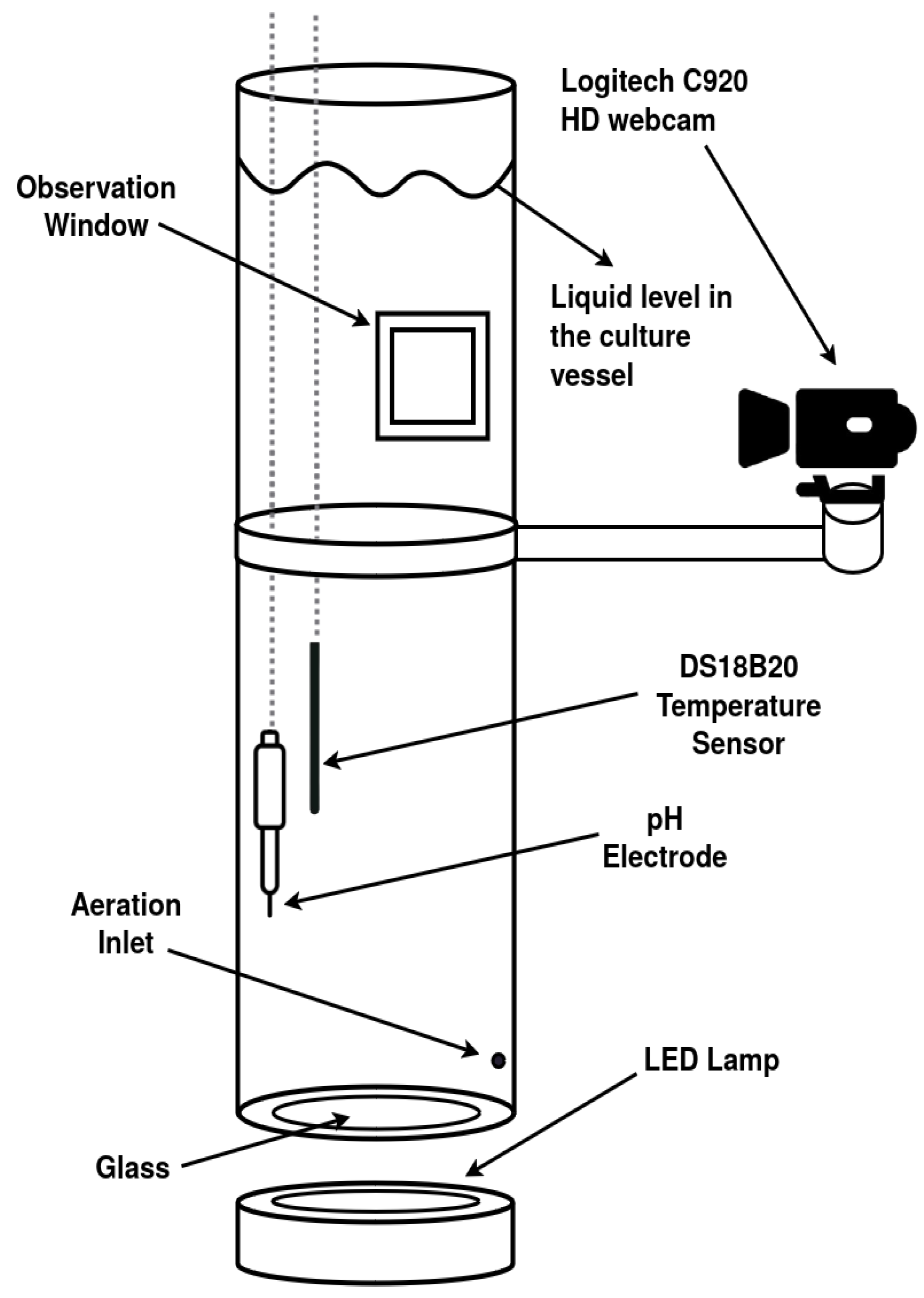
Figure 1. Schematic of the smart photobioreactor with sensor and camera placement.
Eng 06 00221 g001
Figure 2. Wiring diagram of the ESP32 based acquisition and control system.
Eng 06 00221 g002
Figure 3. Block diagram of the proposed four-stage monitoring and control framework.
Eng 06 00221 g003
Figure 4. Smart bioreactor: (Left) inactive state, empty with no illumination; (Right) operational state, showing suspended Chlorella vulgaris and green LED lighting.
Eng 06 00221 g004
Figure 5. Distribution analysis of pH and temperature data before and after IQR outlier filtering. Histograms and kernel density estimates showing non-normal distributions (Shapiro–Wilk p < 0.001). Filtered distributions maintain similar central tendencies. Boxplots demonstrate outlier removal (1.5 × IQR threshold). Mean values shifted minimally after filtering (temperature: 27.85→27.96 °C; pH: 8.94→9.04).
Eng 06 00221 g005
Figure 6. Principal Component Analysis (PCA) of the 10-dimensional feature space. Two-dimensional projection showing clear separation between growth phases (Lag, Exponential, Stationary), with 95% variance retained. Cumulative explained variance indicating 2 principal components capture >80% of variance. Results confirm that IQR filtering preserved biologically meaningful patterns in the data. PCA was applied solely to confirm feature discriminability (95% variance retained) for the ANN classifier, not to infer biological patterns. The 2D projection (Figure 6) shows clear phase separation, validating the RGBI + sensor fusion for computational phase detection.
Eng 06 00221 g006
Figure 7. Layer-by-layer architecture of the feed-forward ANN classifier.
Eng 06 00221 g007
Figure 8. Class distribution in the raw dataset. Stationary phase dominates (70.8%), reflecting typical cultivation dynamics where cells spend prolonged periods in nutrient-limited states. Exponential (18.1%) and lag (11.1%) phases are underrepresented but critical for early intervention.
Eng 06 00221 g008
Figure 9. Specific growth rates (μ) derived from luminance (I) for three C. vulgaris cultures. Dashed lines indicate μ_max (0.0407–0.1365 h−1), calculated during exponential phase.
Eng 06 00221 g009
Figure 10. Biomass proxy (1—normalized I) vs. time. Inverted I values simulate optical density trends, with Culture 2 showing atypical decline post-exponential phase, potentially indicating stress.
Eng 06 00221 g010
Figure 11. Average learning curves: loss (left) and accuracy (right) for training vs. validation (40 runs).
Eng 06 00221 g011
Figure 12. Mean ROC curves for the three classes across the 40 runs.
Eng 06 00221 g012
Figure 13. Normalised confusion matrix averaged over 40 runs. Diagonal cells indicate correct classifications, while off-diagonal cells correspond to misclassifications between classes.
Eng 06 00221 g013
Figure 14. Degradation of model accuracy under controlled perturbations.
Eng 06 00221 g014
Figure 15. Evolution of light absorbance (RGBI means) throughout the 98-day cultivation experiment.
Eng 06 00221 g015
Table 1. Input feature scheme and normalization ranges used for the neural network.
No.FeatureSymbolObserved Range*Normalization MethodNormalized Range
1Mean red intensity R ¯ 1.8–249.9 (8-bit)Z-score (μ = 32.2, σ = 62.9)−0.4–+3.4
2Mean green intensity G ¯ 1.8–252.9 (8-bit)Z-score (μ = 64.8, σ = 84.4)−0.7–+2.2
3Mean blue intensity B ¯ 1.6–251.7 (8-bit)Z-score (μ = 45.6, σ = 69.7)−0.6–+2.9
4Mean perceptual luminance I ¯ 1.8–251.2 (8-bit)Z-score (μ = 55.3, σ = 76.6)−0.7–+2.5
5Red channel std. dev.σR0.3–37.5 (8-bit)Min–max0–1
6Green channel std. dev.σG0.3–39.3 (8-bit)Min–max0–1
7Blue channel std. dev.σB0.2–43.0 (8-bit)Min–max0–1
8Luminance std. dev.σI0.2–35.9 (8-bit)Min–max0–1
9Mean pHpHmean7.20–10.40Min–max0–1
10Mean temperature (°C)Tmean21.69–31.31Min–max0–1
Table 2. Overall classification performance (mean ± standard deviation) obtained with 5-fold stratified.
MetricLag PhaseExponential PhaseStationary PhaseMacro Average
Accuracy0.99230.96650.99970.9862
Recall0.99200.99410.99240.9928
F1-score0.99200.97990.99600.9893
AUC-ROC0.99990.99970.99990.9999
Table 3. Computational performance metrics on the training computer (average of 40 experiments).
MetricMean ValueStandard Deviation
CPU Usage (%)22.41.2
RAM Consumption (MB)2450950
Training Time per Epoch (s)9.81.5
Inference Latency (ms)1345
Table 4. Computational performance metrics of the model on the ESP32 microcontroller.
MetricMean ValueDescription
Model size13.48 KB8-bit quantized model (TFLite Micro format)
Processor frequency240 MHzESP32 dual-core (Xtensa LX6, no operating system)
Inference latency4.8 msAverage time per sample (measured directly on the embedded environment)
Speed-up vs. PC environment×28Compared to single-sample validation inference (134 ms on PC)
Tensor arena usage2 KBMemory allocated for internal model tensors
Estimated total RAM usage<25 KBIncludes model, tensors, stack, and auxiliary buffers
Available memory (SRAM)~520 KBOn standard ESP32 versions (without external PSRAM)
Estimated CPU usage~24%Assuming 50 inferences per second (continuous operation)
Model accuracy98%Maintained after quantization and deployment on embedded device
Table 5. Comparative analysis between this study and prior research on microalgae classification and monitoring.
StudyDomain/TaskModel and PlatformAccuracy/mAPEmbedded InferenceInference LatencyΔ Accuracy vs. Ours
This study Microalgae growth-phase classificationDense network—ESP32 (TFL-Micro)0.9862Yes4.8 ms
[41]Optical density prediction from imagesDNN—PC0.9600*NoNA+2.6 pp
[44]Morphological classification via microscopyCNN/SVM—PC0.9500*NoNA+3.6 pp
[45]Systematic review: algae detectionVarious (CNN, SVM)—PC0.9997* (máximo)NoNA–1.3 pp
[42]Cancer prognosis via algae algorithmCNN-XGBoost—PC0.9900NoNA–0.4 pp
[38]Algae species classification (13 classes)CNN + SENet—PC0.9390NoNA+4.7 pp
[46]Detection/growth/utilizationCNN, RF, SVM—PC0.9200*NoNA+6.2 pp
[33]Algal taxonomy (16 genera)ResNeXt—GPU0.9997NoNA–1.3 pp
[35]Growth monitoring (Spirulina)ANN—Arduino0.9522*NoNA+3.4 pp
[40]Morphological classificationAlexNet—PC0.9600NoNA+2.6 pp
[47]Cyanobacteria quantification (PC/Chl-a)PRCNN—PC (hyperspectral)0.8600*NoNA+12.6 pp
[39]FlowCAM-based algae classificationCNN—PC0.8859NoNA+10.3 pp
Disclaimer/Publisher’s Note: The statements, opinions and data contained in all publications are solely those of the individual author(s) and contributor(s) and not of MDPI and/or the editor(s). MDPI and/or the editor(s) disclaim responsibility for any injury to people or property resulting from any ideas, methods, instructions or products referred to in the content.