A BEM Adjoint-Based Differentiable Shape Optimization of a Stealth Aircraft

Abstract

Modern fighter aircraft have an increasing need for at least a moderate level of stealth, and the shape design must bear a part of this constraint. However, the high frequency of close range radar makes high-fidelity radar cross-section computation methods such as the boundary element method too expensive to use in a gradient-free optimization process. On the other hand, asymptotic methods are not able to accurately predict the RCS of complex shapes such as intake cavities. Hence, the need arises for efficient and accurate methods to compute the gradient of high-fidelity radar cross-section computation methods with respect to shape parameters. In this paper, we propose an adjoint formulation for the boundary element method to efficiently compute these gradients. We present a novel approach to calculate the gradient of high-fidelity radar cross-section computations using the boundary element method. Our method employs an adjoint formulation that allows for the efficient computation of these gradients. This is particularly beneficial in shape optimization problems where accurate and efficient methods are crucial to designing modern fighter aircraft with stealth capabilities. By avoiding the need for solving the actual adjoint problem in certain cases, our formulation provides a more streamlined solution while still maintaining high accuracy. We demonstrate the effectiveness of our method by performing shape optimization on various shapes, including simple geometries like spheres and ellipsoids, as well as complex aircraft shapes with multiple variables.

1. Introduction

With the widespread use of radar technology in various applications, including early detection, target acquisition by air defense systems, and active radar homing for missiles, modern fighter aircraft design must consider stealth as a critical factor. Stealth technology aims to minimize the radar cross-section (RCS) of an object, which is a measure of its reflectivity and visibility to radar. A lower RCS reduces the detection range of the aircraft, providing a shorter reaction time to hostile defense systems.

The frequency bands commonly used by modern radars are the UHF, L, S, C, and X bands [1]. Their working frequencies range from $300\mathrm{MHz}$ to $12\mathrm{GHz}$, corresponding to wavelengths between $0.025\mathrm{m}$ and $30\mathrm{c}\mathrm{m}$, which are much smaller than typical aircraft dimensions. Therefore, the radar waves are considered high-frequency. This means that the scattering characteristics of the aircraft are heavily influenced by its geometry.

High-frequency methods, such as Physical Optics (PO), usually allows for an acceptable accuracy when predicting the RCS for a preliminary industrial shape design. In a previous study [2], we investigated the use of PO in order to perform aero-stealth optimization. In the long run, however, PO is unable to deal with multi-reflection or cavity resonance, which are necessary to accurately predict the RCS of a more complex shape, and the use of a high-fidelity method such as the boundary element method (BEM) appears unavoidable.

Gradient-free optimization algorithms have the advantage of not necessitating the costly computation of derivatives, which can be hard to derive or implement. However, they need a high number of objective function evaluations, whose computation may be prohibitive when using high-fidelity solvers. In an industrial design process, gradient-free algorithms are typically used for preliminary design with low-fidelity models, while gradient-based methods are more adapted to large-scale aircraft shape design with mid- to high-fidelity models. Furthermore, surrogate-based algorithms are known to struggle with constraint handling, satisfying them with a poor accuracy and stopping criteria [3].

1.1. Gradient-Based Optimization

Gradient-based optimization methods have been widely recognized for their efficiency in reducing the number of function evaluations compared to gradient-free methods. This is particularly evident when dealing with complex problems that involve a high dimension of optimization parameters. For instance, Lyu et al. [4] benchmarked various optimization algorithms, both gradient-free and gradient-based, on three different problems with increasing complexity. They demonstrated that while gradient-free methods tend to require more function evaluations as the number of optimization parameters increases, gradient-based methods maintain a linear behavior. This becomes increasingly significant when the design space has more than ten dimensions. In such cases, gradient-free algorithms may need tens or hundreds of thousands of function evaluations, whereas gradient-based algorithms using an analytic method like the adjoint formulation to compute the gradient require less than a hundred.

The adjoint formulation of the problem allows for an efficient computation of the gradient of the objective and constraints with respect to the optimization parameters. For the applications of this study, the cost of the gradient computation is roughly linear with respect to the number of design variables and the size of the mesh. Various publications have already covered the application of the adjoint method to gradient-based optimization. For instance, Martin applied the adjoint method to robust airfoil optimization [5]. Martin used the automatic differentiation (AD) tool TAPENADE [6] to develop his discrete adjoint solver, which drastically reduced the implementation time.

1.2. The Boundary Element Method

A full-wave method numerically solves the Maxwell equations, without any preliminary physical hypothesis. The BEM, sometimes designed as a Method of Moments (MoM), is one of the three main full-wave methods, along with the finite-element method (FEM) and Finite-Difference Time-Domain method (FDTD). Full-wave techniques can be very accurate and rely on the discretization of some unknown quantity. In the case of the BEM, the current distribution, generally a surface current distribution, is discretized into segments or patches, whose interactions between each other are represented by a matrix computed using the Green function of the problem. This allows us to only discretize the surface rather than the whole volumic domain, but at the cost that the matrix is then densely populated. With the relevant boundary conditions applied to the interactions, this yields a set of linear equations whose solution is the current on each segment or patch. Additionally, the radiation condition is built into the BEM, which means that it accurately describes the far field and no special treatment is required to handle unbounded domains, making it ideal for scattering problems such as the one of this study. This is not true for the FEM or FDTD.

The BEM, however, does not efficiently handle non-perfect electric conductor (PEC) materials, especially if they are not homogeneous, when compared to the FDTD or FEM, though this can be worked around by applying a local penalty on the impedance of the material. In the case of inhomogeneous material, a volume mesh is needed, which is dramatically detrimental to the efficiency of the method. This limitation is not a big deal as non-electrically perfect materials are beyond the scope of this study.

Naturally, the accuracy of the method depends heavily on the fineness of the discretization. Typically for the BEM, a step size of around $\lambda /10$ to $\lambda /5$ is used, with $\lambda$ being the wavelength. This means that the BEM scales poorly with increasing frequencies, with an upper bound of $\mathcal{O}\left(f^6\right)$ ($\mathcal{O}\left(f^9\right)$ in the case of a volume mesh) [7]. This drastically limits the range of frequencies computable with this method, especially in an optimization framework.

For a more in-depth discussion on the various full-wave methods, their limitations, and how they compare to one another, please refer to [7].

1.3. Electromagnetic Gradient-Based Optimization

Various studies have already tackled the problem of electromagnetic shape optimization using gradient-based methods. Bardos and Roge [8] applied the optimal control theory of Lions [9] to control the backscattered field around an aircraft shape. Paoli [10] derived a continuous adjoint formulation for the BEM and applied it to constrained optimization, and Roge applied her method to stealth shape optimization [11]. Georgieva [12,13] proposed a continuous adjoint formulation for frequency-domain sensitivity computation and applied it to antenna design. Wang and Anderson [14] also contributed to this field by applying the discontinuous Galerkin (DG) method to solve electromagnetic problems and employing a time-dependent discrete adjoint method to obtain sensitivity derivatives. They used the gradient computed by the adjoint method to control the magnetic field at the surface of an airfoil over time.

Recently, Zhou et al. used a BEM and its adjoint to perform the 3D aero-stealth optimization of a UCAV shape [15]. They used a CAD-less solution called Free-Form Deformation to pilot the shape, and they computed the RCS by solving the BEM problem with an iterative solver, and its gradient with an adjoint formulation for the BEM.

Very recently, Cheng et al. used the Singular Boundary Method (SBM) and its adjoint to perform 2D and 3D sensitivity acoustic analysis [16], which was extended in the 2D case by Lan et al. to the use of ACA compression to decrease both computation time and memory requirements [17]. Finally, Liu et al. used this method to perform a 2D acoustic shape optimization of a sound barrier geometry represented by B-spline [18]. The SBM is a relatively new, semi-analytical variant of the BEM whose particularity is to avoid the use of a mesh or of numerical integration. It was introduced for the first time by Chen et al. in 2009 [19]. It has seen limited use in Computational ElectroMagnetism (CEM) (see, for example [20]), but is still limited to 2D or low-frequency 3D problems with simple geometries, and the BEM remains, for the moment, the preferred method for 3D scattering problems with PEC obstacles.

1.4. Contributions

The resolution of a BEM for a realistic L through X band radar is very expensive, especially in the frame of an optimization process. However, the purpose of this study is to formulate an adjoint formulation for the BEM system in order to perform gradient-based optimization and to demonstrate the feasibility of such a process, in an industrial framework, on increasingly complex shapes.

In this framework, we introduce the use of a CAD modeler, whose advantages are expended upon in Section 3.1. We also introduce the use of an automatic differentiation tool, as presented in Section 3.2. Finally, we present an adjoint formulation for the BEM and show that with the correct formulation, the actual resolution of the adjoint system is not necessary.

This paper is organized as follows. First, we derive the BEM and formulate its adjoint system in Section 2. In Section 3, we present the optimization process and its most relevant modules. Then, in Section 4, we validate the solver and its gradient and showcase the algorithm process on simple geometries such as a sphere and an ellipsoid. Afterwards, in Section 5, we present a more ambitious optimization of a simplified aircraft shape with many variables. Finally, in Section 6, we present our conclusions and discuss how to improve upon this experiment.

2. RCS, BEM, and Adjoint Formulation

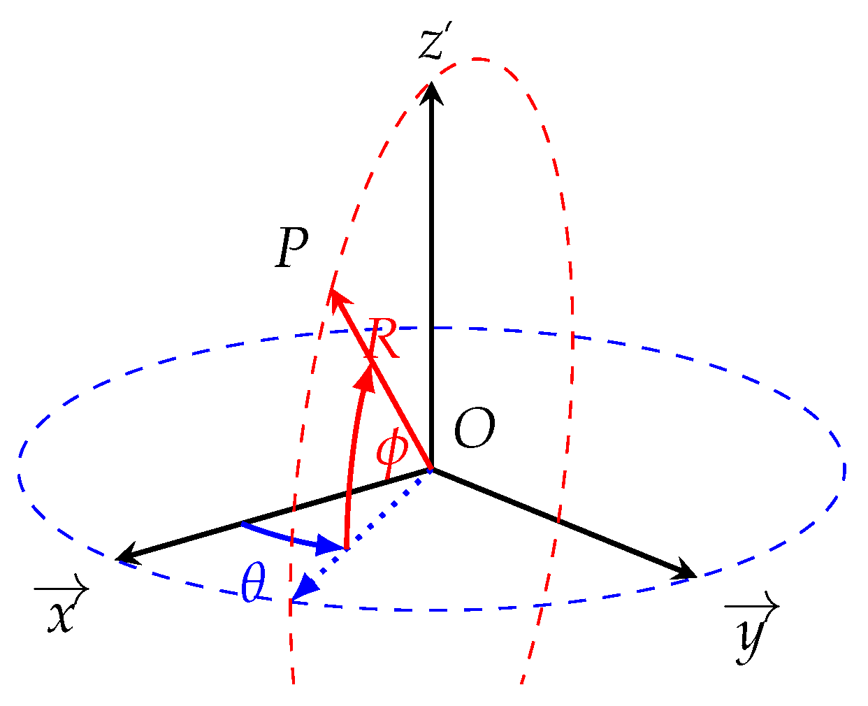
2.1. The Radar Cross-Section

Aircraft must meet a number of criteria in order to be considered stealthy. Here, we will only deal with the capacity of the aircraft to scatter a limited amount of energy back into the direction of the emitter. We only consider a monostatic radar, which represents the large majority of the systems in use. This means that the emitting antenna and the receiving antenna are collocated. A popular measure of the scattered electromagnetic energy is the radar cross-section (RCS) $\sigma$ defined as follows:

$$\sigma (\theta ,\varphi )=\underset{R\to \infty }{lim}{R}^2{\displaystyle \frac{|{\mathbf{E}}_P{|}^2}{|{\mathbf{E}}_i{|}^2}},$$

(1)

where ${\mathbf{E}}_P$ denotes the scattered electric fields at a point $P(R,\theta ,\varphi )$ in polar coordinates, and ${\mathbf{E}}_i$ is the incident electric field. The bearing ($\theta$) and elevation ($\varphi$) angles are defined in Figure 1. Usually, the RCS is expressed in decibels:

$${\sigma }_{\mathrm{dB}}=10log\left(\sigma \right).$$

In order to derive the RCS, one must first be able to compute the electric field scattered by a target.

2.2. Far Field

Let us recall the Maxwell equations in a homogeneous, lossless medium $\Omega$, considering a harmonic regime whose wave number is k:

$$\nabla ·\mathbf{D}=\varrho ,$$

(2a)

$$\nabla ·\mathbf{B}=0,$$

(2b)

$$\nabla \times \mathbf{E}=j\omega \mathbf{B}-\mathbf{M},$$

(2c)

$$\nabla \times \mathbf{H}=\mathbf{J}-j\omega \mathbf{D},$$

(2d)

where $\mathbf{D}={\epsilon }_0\mathbf{E}$, $\mathbf{H}=\mathbf{B}/{\mu }_0$, and $\omega ={\displaystyle \frac{k{\mu }_0}{Z_0}}$, with ${\epsilon }_0$ as the permittivity of the vacuum, ${\mu }_0$ as the permittivity of the vacuum, $\varrho$ as the density of electric charges, and $\mathbf{J}$ and $\mathbf{M}$ as, respectively, the density of the electric and magnetic current.

Since the medium is homogeneous, it is only necessary to compute $\mathbf{E}$, since $\mathbf{H}$ can then be derived from (2c):

$$\mathbf{H}={\displaystyle \frac{Z_0}{jk{\mu }_0}}\left(\nabla \times \mathbf{E}+\mathbf{M}\right).$$

(3)

From this, $\mathbf{H}$ can be eliminated from (2d):

$$\nabla \times \nabla \times \mathbf{E}-k^2\mathbf{E}=jk{Z}_0\mathbf{J}-\nabla \times \mathbf{M}.$$

(4)

By computing the divergence of, (4)

$$\nabla ·\mathbf{E}=-j{\displaystyle \frac{Z_0}{k}}\nabla ·\mathbf{J},$$

(5)

and using the well-known formula

$$\nabla \times \nabla \times A=\nabla \nabla ·A-{\nabla }^{2}A,$$

(6)

it is possible to decouple the equations for each component in (4) and obtain the 3D vector Helmholtz equation:

$$-\left({\nabla }^2+k^2\right)\mathbf{E}=-jk{Z}_0\left({\displaystyle \frac{1}{k^2}}\nabla \nabla ·+1\right)\mathbf{J}-\nabla \times \mathbf{M}.$$

(7)

Let us define

$$\mathbf{T}=k{Z}_0\left({\displaystyle \frac{1}{k^2}}\nabla \nabla ·+1\right)\mathbf{J}-\nabla \times \mathbf{M}.$$

(8)

Equation (7) has a well-known solution that is $C^{\infty }$ outside the support of $\mathbf{T}$ and can be expressed as

$$\mathbf{E}\left(x\right)={\int }_{\Omega }\mathbf{T}\left(y\right)G(x,y)\mathrm{d}\Omega \left(y\right),\forall x\notin \mathrm{supp}\left(\mathbf{T}\right),$$

(9)

where G is the Green kernel for the Helmholtz equation (for more details, see [21], particularly Chapter 2).

$$G(x,y)={\displaystyle \frac{e^{-jk∥x-y∥}}{∥x-y∥}}.$$

(10)

It can be shown that in the case where the support of $\mathbf{T}$ is compact, solution (9) can be expressed as a Taylor development:

$$\mathbf{E}\left(x\right)={\displaystyle \frac{e^{jk∥x∥}}{∥x∥}}\left\{{\mathbf{E}}^{\infty }\left({\displaystyle \frac{x}{∥x∥}}\right)+\mathcal{O}\left({\displaystyle \frac{1}{∥x∥}}\right)\right\},$$

(11)

where

$${\mathbf{E}}^{\infty }\left({\mathbf{u}}_s\right)={\displaystyle \frac{jk}{4\pi }}{\mathbf{u}}_s\times \left(Z_0\mathcal{F}\left(\mathbf{J}\right)\left({\mathbf{u}}_s\right)\times {\mathbf{u}}_s-\mathcal{F}\left(\mathbf{M}\right)\left({\mathbf{u}}_s\right)\right),$$

(12)

is the far field in the direction ${\mathbf{u}}_s$. The quantity $\mathcal{F}\left(\mathbf{P}\right)\left(\mathbf{u}\right)$ is the radiation function associated with a compact support vector distribution $\mathbf{P}$ in direction $\mathbf{u}$, and it is defined as

$$\mathcal{F}\left(\mathbf{P}\right)\left({\mathbf{u}}_s\right)={\int }_{\Omega }\mathbf{P}\left(y\right)e^{jk{\mathbf{u}}_s·y}\mathrm{d}\Omega \left(y\right),$$

(13)

Equation (11) shows that the limit in (1) exists and depends only on the far field ${\mathbf{E}}^{\infty }$:

$$\sigma \left({\mathbf{u}}_s\right)=4\pi \underset{R\to \infty }{lim}{R}^2{\displaystyle \frac{{∥\mathbf{E}\left(R{\mathbf{u}}_s\right)∥}^2}{{∥{\mathbf{E}}^{\mathrm{inc}}∥}^2}}=4\pi {∥{\mathbf{E}}^{\infty }\left({\mathbf{u}}_s\right)∥}^2.$$

(14)

Let ${\mathbf{u}}_s$ and $\widehat{\mathit{\tau }}$ be unit vectors so that ${\mathbf{u}}_s\perp \widehat{\mathit{\tau }}$. For reasons that will be explained in Section 2.3, we consider $\mathbf{M}$ to be zero. We define the RCS of the far field in direction ${\mathbf{u}}_s$, polarized along direction $\widehat{\mathit{\tau }}$ as follows:

$$\sigma (\widehat{\mathit{\tau }},{\mathbf{u}}_s)=4\pi {\left|\widehat{\mathit{\tau }}·{\mathbf{E}}^{\infty }\left({\mathbf{u}}_s\right)\right|}^2={\displaystyle \frac{k^2{Z}_0^2}{4\pi }}{\left|{\int }_{\Omega }\widehat{\mathit{\tau }}·\mathbf{J}\left(y\right)e^{jk{\mathbf{u}}_s·y}\mathrm{d}\Omega \left(y\right)\right|}^2.$$

(15)

2.3. The Electric Field Integral Equation

Consider a warped, airtight surface $\Gamma$ representing the target immersed in an unbounded free space domain $\Omega$. Let $\mathbf{n}$ be the outward-pointing normal unit vector to $\Gamma$. Consider also an incident plane wave $\left({\mathbf{E}}^{\mathrm{inc}},{\mathbf{H}}^{\mathrm{inc}}\right)$ propagating along direction ${\mathbf{u}}_i$ and $\left({\mathbf{E}}^{+},{\mathbf{H}}^{+}\right)$ the total electromagnetic field. As shown in Section 2.2, the RCS of the target $\Gamma$ depends only on the current distribution induced on it by the incident field.

The incident electric field at point x can be written as

$${\mathbf{E}}^{\mathrm{inc}}=\widehat{\mathit{\tau }}{e}^{jk{\mathbf{u}}_i·x},$$

with $\widehat{\mathit{\tau }}\perp {\mathbf{u}}_i$ and $∥\widehat{\mathit{\tau }}∥=1\mathrm{V}/\mathrm{m}$. Furthermore, since $\Omega \backslash \Gamma$ is a vacuum, this means that $\mathbf{J}{|}_{\Omega \backslash \Gamma }=\mathbf{0}$.

The total electric field at point $x\in \Omega \backslash \Gamma$ can be expressed with the Stratton–Chu formula [22]:

$${\mathbf{E}}^{+}={\mathbf{E}}^{\mathrm{inc}}+jk{Z}_0\mathcal{T}\mathbf{J}+\mathcal{K}\mathbf{M}$$

(16)

where $\mathcal{T}\mathbf{J}$ and $\mathcal{K}\mathbf{M}$ are the potentials associated, respectively, with $\mathbf{J}$ and $\mathbf{M}$ defined for $x\notin \Gamma$.

$$\left(\mathcal{T}\mathbf{J}\right)\left(x\right)=\left({\displaystyle \frac{1}{k^2}}{\nabla }_{\Gamma }{\nabla }_{\Gamma }·+1\right){\int }_{\Gamma }G(x,y)\mathbf{J}\left(y\right)\mathrm{d}\Gamma \left(y\right),x\notin \Gamma$$

(17a)

and

$$\left(\mathcal{K}\mathbf{M}\right)\left(x\right)=-\nabla \times {\int }_{\Gamma }G(x,y)\mathbf{M}\left(y\right)\mathrm{d}\Gamma \left(y\right),x\notin \Gamma ,$$

(17b)

with G being the Green kernel defined in Equation (10).

Physically, the magnetic current density $\mathbf{M}$ is zero, though the consideration of this fictive quantity may simplify some modelization problems. From this point on, $\mathbf{M}$ is considered zero.

We assume that the target is a perfect electric conductor (PEC):

$${\mathbf{E}}^{+}\left(x\right)\times \mathbf{n}=\mathbf{0},\forall x\in \Gamma .$$

(18)

The tangent trace of $\mathcal{T}\mathbf{J}$ is continuous across $\Gamma$ and $\forall x\in \Gamma$:

$$\left(\mathcal{T}\mathbf{J}\right)\left(x\right)\times \mathbf{n}={\displaystyle \frac{1}{k^2}}{\nabla }_{\Gamma }{\int }_{\Gamma }G(x,y){\nabla }_{\Gamma }·\mathbf{J}\left(y\right)\mathrm{d}\Gamma \left(y\right)+\left({\int }_{\Gamma }G(x,y)\mathbf{J}\left(y\right)\mathrm{d}\Gamma \left(y\right)\right)\times \mathbf{n}.$$

(19)

Therefore, applying the PEC condition (18) to the total electric field (16) yields

$$\mathcal{T}\mathbf{J}\times \mathbf{n}={\displaystyle \frac{1}{jk{Z}_0}}{\mathbf{E}}^{\mathrm{inc}}\times \mathbf{n}$$

(20)

It is more convenient to express Equation (20) as a variational problem. To do so, it is first necessary to introduce the space

$$H_{\mathrm{div}}(\Gamma ):=\left\{\mathbf{J}\in L^2(\Gamma ;{\mathbb{C}}^3),\mathbf{J}\times \mathbf{n}=\mathbf{0},{\nabla }_{\Gamma }·\mathbf{J}\in L^2(\Gamma )\right\}.$$

The variational problem is the following:

$$\left\{\begin{array}{ccc}\hfill & \mathrm{Find}\mathbf{J}\in H_{\mathrm{div}}(\Gamma ),\forall \mathbf{\Psi }\in H_{\mathrm{div}}(\Gamma ),\hfill & \\ \hfill {\displaystyle \frac{j}{4\pi }}{\int }_{\Gamma }{\int }_{\Gamma }kG(x,y)& \left(-{\displaystyle \frac{1}{k^2}}{\nabla }_{\Gamma }·\mathbf{\Psi }\left(x\right){\nabla }_{\Gamma }·\mathbf{J}\left(y\right)+\mathbf{\Psi }\left(x\right)·\mathbf{J}\left(y\right)\right)\mathrm{d}\Gamma \left(y\right)\mathrm{d}\Gamma \left(x\right)\hfill & \\ & ={\int }_{\Gamma }\mathbf{\Psi }\left(y\right)·\left({\displaystyle \frac{1}{Z_0}}{\mathbf{E}}^{\mathrm{inc}}\left(y\right)\right)\mathrm{d}\Gamma \left(y\right).\hfill \end{array}\right.$$

(21)

This form of the problem is called the Electric Field Integral Equation (EFIE). It is a linear system that can be written as

$$\left\{\begin{array}{c}\mathrm{Find}\mathbf{J}\in H_{\mathrm{div}}(\Gamma ),\forall \mathbf{\Psi }\in H_{\mathrm{div}}(\Gamma ),\\ \mathcal{A}(\mathbf{J},\mathbf{\Psi })=\ell (\mathbf{\Psi }),\end{array}\right.,$$

(22)

where $\mathcal{A}:H_{\mathrm{div}}(\Gamma )\times H_{\mathrm{div}}(\Gamma )\to \mathbb{C}$ is a symmetric bilinear form, and $\ell :H_{\mathrm{div}}(\Gamma )\to \mathbb{C}$ is a linear form.

Problem (21) is well-posed except for an increasing discrete sequence of values of k corresponding to the resonance frequencies of the interior of $\Gamma$:

$$k\notin \left\{k_i^c,i\in \mathbb{N}\right\}.$$

However, in the case of the critical values $k_i^c$, the solution is defined within one solution to the homogeneous equation, which are called parasitic currents. Since these currents do not radiate to the outside, the computation of the RCS remains stable.

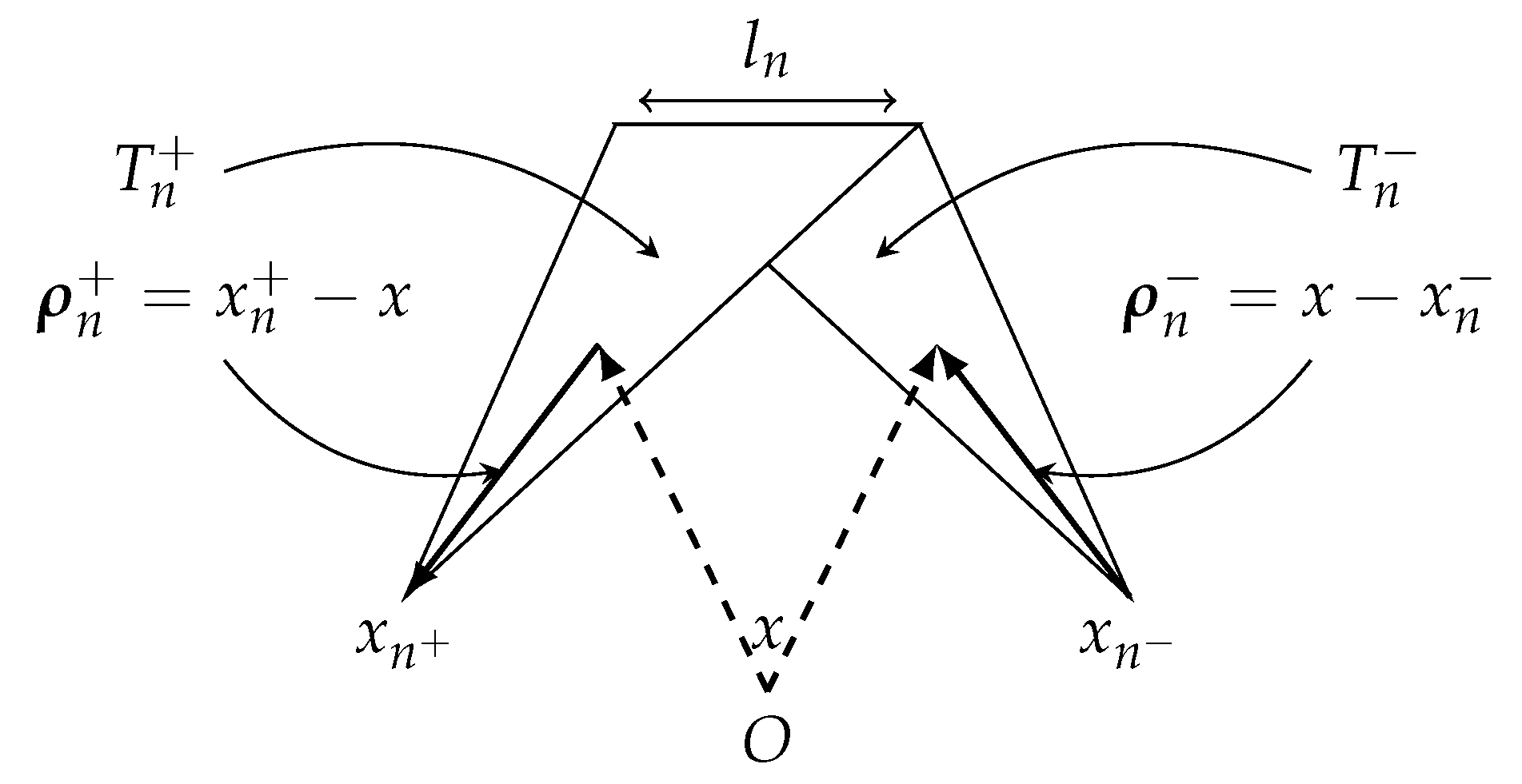
2.4. The Boundary Element Method

In this section, we approximate the surface $\Gamma$ with triangular finite elements. From now on, $\Gamma$ will refer to the discretized shape. Finally, let $T\in \Gamma$ denote a triangle T on $\Gamma$, and $l_i$ the $i^{\mathrm{th}}$ edge of T.

Let us number the edges 1 through N and define an orientation for each one in order to distinguish the pair of triangles delimited by each edge n as a triangle $T_n^{+}$ and a triangle $T_n^{-}$. It is possible to write the field $\mathbf{J}$ as

$$\mathbf{J}\left(x\right)=\sum _{n=1}^N{I}_n{\mathbf{f}}_n\left(x\right),$$

(23)

where components $I_{n_{T,i}}$ are linked to the $J_{T,i}$ through the relation

$$I_{n_{T,i}}={ϵ}_{T,i}{J}_{T,i},$$

with

$${ϵ}_{T,i}=\left\{\begin{array}{cc}\hfill 1& \hfill \mathrm{if}T=T_{n_{T,i}}^{+},\\ \hfill -1& \hfill \mathrm{if}T=T_{n_{T,i}}^{-}.\end{array}\right.$$

The functions ${\mathbf{f}}_n$ used in Equation (23) are the Rao–Wilton–Glisson (RWG) basis functions [23], defined as follows:

$${\mathbf{f}}_n\left(x\right)=\left\{\begin{array}{cc}{\displaystyle \frac{l_n}{S_n^{-}}}\left(x-x_n^{-}\right)\hfill & \hfill \mathrm{if}x\in T_n^{-},\\ {\displaystyle \frac{l_n}{S_n^{+}}}\left(x_n^{+}-x\right)\hfill & \hfill \mathrm{if}x\in T_n^{+},\end{array}\right.$$

(24)

with $S_n^{\pm }$ as the area of the triangle $T_n^{\pm }$ (see Figure 2).

Consider the subspace

$$X^h\left\{\mathbf{J}\in H_{\mathrm{div}}(\Gamma ),\forall T\in \Gamma ,\mathbf{J}{|}_T=J_{T,1}{\mathbf{f}}_{T,1}+J_{T,2}{\mathbf{f}}_{T,2}+J_{T,3}{\mathbf{f}}_{T,3}\right\},$$

(25)

where the local components $J_{T,i}$ are the fluxes across edge $l_i$.

With this finite-element method, it is now possible to discretize the EFIE. This method is called the BEM, or sometimes the Method of Moments (MoM):

$$\left\{\begin{array}{ccc}\hfill & \mathrm{Find}\mathbf{J}\in X^h,\forall \mathbf{\Psi }\in X^h,\hfill & \\ \hfill {\displaystyle \frac{j}{4\pi }}{\int }_{\Gamma }{\int }_{\Gamma }kG(x,y)& \left(-{\displaystyle \frac{1}{k^2}}{\nabla }_{\Gamma }·\mathbf{\Psi }\left(x\right){\nabla }_{\Gamma }·\mathbf{J}\left(y\right)+\mathbf{\Psi }\left(x\right)·\mathbf{J}\left(y\right)\right)\mathrm{d}\Gamma \left(y\right)\mathrm{d}\Gamma \left(x\right)\hfill & \\ & ={\int }_{\Gamma }\mathbf{\Psi }\left(y\right)·\left({\displaystyle \frac{1}{Z_0}}{\mathbf{E}}^{\mathrm{inc}}\left(y\right)\right)\mathrm{d}\Gamma \left(y\right).\hfill \end{array}\right.$$

(26)

Usually, this variational problem is written as a linear system:

$$AI=b,$$

(27)

where I is the vector of the unknowns of $\mathbf{J}$ and A is a symmetric, non-Hermitian, matrix.

2.5. The Adjoint Formulation

2.5.1. Continuous Formulation

Consider that the target is represented by a surface parameterized by p parameters and let $\eta \in {\mathbb{R}}^p$ be a vector of the values of said parameters. The target is approximated by a polyhedral surface $\Gamma$ whose node positions are noted $X\left(\eta \right).$ The derivative ${\displaystyle \frac{\partial X}{\partial \eta }}$ is computed with the CAD modeler presented in Section 3.1 and is supposedly known at this stage.

We write the linear system for which $\mathbf{J}$ is unknown and defined in Equation (21) as a function of X and $\mathbf{J}$:

$$\mathcal{R}\left(X\right(\eta ),\mathbf{J}(\eta \left)\right)=0.$$

Given a complex observation function

$$\zeta \left(X\right(\eta ),\mathbf{J}(\eta \left)\right)\in \mathbb{C},$$

the differential of $\zeta$ is

$$\mathrm{d}\zeta =\left({\displaystyle \frac{\partial \zeta }{\partial X}}{\displaystyle \frac{\partial X}{\partial \eta }}+{\displaystyle \frac{\partial \zeta }{\partial \mathbf{J}}}{\displaystyle \frac{\partial \mathbf{J}}{\partial \eta }}\right)\mathrm{d}\eta .$$

(28)

The term ${\displaystyle \frac{\partial \mathbf{J}}{\partial \eta }}$ is costly to compute, but since

$$\mathrm{d}\mathcal{R}=\left({\displaystyle \frac{\partial \mathcal{R}}{\partial X}}{\displaystyle \frac{\partial X}{\partial \eta }}+{\displaystyle \frac{\partial \mathcal{R}}{\partial \mathbf{J}}}{\displaystyle \frac{\partial \mathbf{J}}{\partial \eta }}\right)\mathrm{d}\eta =0,$$

it is possible to write the following formally:

$${\displaystyle \frac{\partial \mathbf{J}}{\partial \eta }}=-{\left({\displaystyle \frac{\partial \mathcal{R}}{\partial \mathbf{J}}}\right)}^{-1}{\displaystyle \frac{\partial \mathcal{R}}{\partial X}}{\displaystyle \frac{\partial X}{\partial \eta }}.$$

(29)

Applying this to Equation (28) yields

$$\mathrm{d}\zeta =\left({\displaystyle \frac{\partial \zeta }{\partial X}}{\displaystyle \frac{\partial X}{\partial \eta }}-{\Phi }^{\ast }{\displaystyle \frac{\partial \mathcal{R}}{\partial X}}{\displaystyle \frac{\partial X}{\partial \eta }}\right)\mathrm{d}\eta ,$$

(30)

with $\Phi$ as the solution to the adjoint system to (21):

$${\left({\displaystyle \frac{\partial \mathcal{R}}{\partial \mathbf{J}}}\right)}^{\ast }\Phi ={\left({\displaystyle \frac{\partial \zeta }{\partial \mathbf{J}}}\right)}^{\ast }.$$

(31)

2.5.2. Discrete Formulation

The derivation of the discrete adjoint follows the same general lines. The considered linear system ${\mathcal{R}}_h$ is now the BEM system defined in Equation (27), a matrix system, and the unknown I and RHS b are complex vectors:

$${\mathcal{R}}_h(X,I)=A\left(X\right)I-b\left(X\right)=0,$$

(32)

with $A\in {\mathcal{M}}_N\left(\mathbb{C}\right)$ as a symmetric non-Hermitian matrix and $b\in {\mathbb{C}}^N$. Let us define the discrete observation function as

$$\zeta (X,I)\in \mathbb{C}.$$

Therefore,

$${\displaystyle \frac{\partial {\mathcal{R}}_h}{\partial I}}=A$$

and

$${\displaystyle \frac{\partial {\mathcal{R}}_h}{\partial X}}={\displaystyle \frac{\partial A}{\partial X}}I-{\displaystyle \frac{\partial b}{\partial X}}.$$

Hence, the derivative of $\zeta$ is

$$\mathrm{d}\zeta ={\displaystyle \frac{\partial \zeta }{\partial X}}\mathrm{d}X-{\Psi }^{\ast }\left({\displaystyle \frac{\partial A}{\partial X}}I-{\displaystyle \frac{\partial b}{\partial X}}\right)\mathrm{d}X,$$

(33)

with $\Psi$ as the solution to the adjoint problem to the discrete BEM system (26),

$$\overline{A}\Psi ={\left({\displaystyle \frac{\partial \zeta }{\partial I}}\right)}^{\ast },$$

(34)

because A is symmetric.

2.6. Computation of the Gradient

Let us define an observable $\zeta$

$$\zeta =2\sqrt{\pi }\left({\mathbf{E}}^{\infty }·\widehat{\mathit{\tau }}\right),$$

(35)

so that, the RCS defined in Equation (15) can be written as $\sigma ={\left|\zeta \right|}^2$.

If ${\mathbf{u}}_s$ is a unit vector, then

$${\mathbf{E}}^{\infty }·\widehat{\mathit{\tau }}={\int }_{\Gamma }\mathbf{J}\left(y\right)·\widehat{\mathit{\tau }}{e}^{jk{\mathbf{u}}_s·y}\mathrm{d}\Gamma \left(y\right),$$

(36)

and if ${\mathbf{u}}_s={\mathbf{u}}_i$, then

$${\mathbf{E}}^{\infty }·\widehat{\mathit{\tau }}={\displaystyle \frac{k{Z}_0^2}{2\sqrt{\pi }}}\ell \left(\mathbf{J}\right).$$

(37)

Therefore, the differential of $\zeta$ is

$$\mathrm{d}\zeta ={\displaystyle \frac{k{Z}_0^2}{2\sqrt{\pi }}}\ell \left(\mathrm{d}\mathbf{J}\right).$$

(38)

Hence, the right-hand side of the discrete adjoint system can be written as

$${\displaystyle \frac{\partial \zeta }{\partial I}}={\displaystyle \frac{k{Z}_0^2}{2\sqrt{\pi }}}b.$$

(39)

From this, there is no need to actually solve system (34), and $\Psi$ is

$${\Psi }^{\ast }={\displaystyle \frac{k{Z}_0^2}{2\sqrt{\pi }}}I.$$

(40)

2.7. In Practice

In practice, the term ${\displaystyle \frac{\partial A}{\partial X}}I$ is the most difficult to compute because of the singularities of matrix A. It is also very expensive to compute numerically and to store. For these reasons, we will temporarily neglect it and try to estimate how much it contributes and if the assumption is reasonable.

3. Optimization Methodology

3.1. The CAD Modeler

In order to model and modify the geometry, we used the CAD tool GANIMEDE [24]. In this study, we used some functionalities of GANIMEDE that have not yet been differentiated, which prevented us from using the exact differentiation presented in [24]. The surface is represented by a set of NURBS grids and parameterized with control points. GANIMEDE uses both global and local variables as input. Local variables are the osculating parameters (i.e., position, tangent, and curvature) at a control point. Global variables allow us to modify usual aeronautical design variables such as sweep and twist angles, or the chord of a wing. The advantage of global variables is that they are much more meaningful to an aircraft designer than the position, tangent angle, and stiffness of points along a spline curve. In this study, we used only global variables.

If a surface mesh is associated with the baseline geometry, GANIMEDE will project the mesh onto the deformed geometry and compute the derivatives of the displacement the mesh nodes with respect to the design variables ${\displaystyle \frac{\mathrm{d}\mathbf{x}}{\mathrm{d}\nu }}$ using centered finite difference. Because of the smoothing and other refinement operations performed by the CAD modeler on the NURBS geometry, too small a step size can lead to a bad gradient, so we have to find an optimal step size for each design variable.

GANIMEDE is also able to compute functions of interest such as fuselage volume, wing planform surface area or wing reference surface, as well as their gradient with respect to the design variables.

3.2. Computational Electromagnetism Solver

The BEM is a matrix equation with a dense matrix whose size is proportional to $N^2$, with N being the number of edges in the mesh. Furthermore, in order to accurately represent the current density at the surface of the target, the mesh step must be small enough that it respects Shannon’s theorem [25]. In practice, this means that the maximum step size of the mesh must be in the order of one 5th to one 10th the smallest wavelength. Thus, the size of the matrix to invert is proportional to the square of the wavelength, and for an aircraft the size of a fighter and a frequency in the order of $\mathrm{GHz},$ the matrix can easily represent a hundred million to a billion double-precision float to handle.

In order to numerically solve the BEM system described in Equation (26) and compute the RCS from the current density field, we use an in-house CEM solver called SPECTRE [26]. As stated in Section 1.2, because the BEM involves inverting a densely populated matrix, it is very expensive both in terms of computation time and memory requirements, scaling as $\mathcal{O}\left(f^6\right)$. Though the SPECTRE features of the advanced method compensate for the storage and complexity cost of the method, including ACA matrix compression, an iterative solver, and a fast multipole method [27], we only use the direct solver in order to keep the mathematical formulation and the code differentiation simple. We use FMSlib [28] with GPU acceleration in order to speed up the matrix inversion.

We used the Automatic Differentiation (AD) tool TAPENADE [6] in order to generate a differentiated program from the relevant SPECTRE subroutines, which are able to compute the derivative of the RCS with respect to the design variables. With this tool, it is possible to save a lot of development and debugging time. TAPENADE offers two modes: tangent (or direct) and reverse. Tangent mode computes the directional derivative using the chain rule, from left to right. This mode is immediate to use as it only needs to create a copy of the input code, interleaved with the derivative instructions. Reverse mode is an efficient way of computing the gradient of a high dimensional quantity. When the objective function F is scalar-valued and the dimension of the design variable vector is large, and assuming that the storage capacity is available, it is theoretically more efficient to compute the Jacobian matrix $\nabla F$ of F row by row and then compute the directional derivative $\mathrm{d}{F}_e=\nabla F_e\mathrm{d}\xi$ rather than to compute it using the chain rule with the direct mode.

Both modes are used for different subroutines depending on the respective dimension of their inputs and outputs.

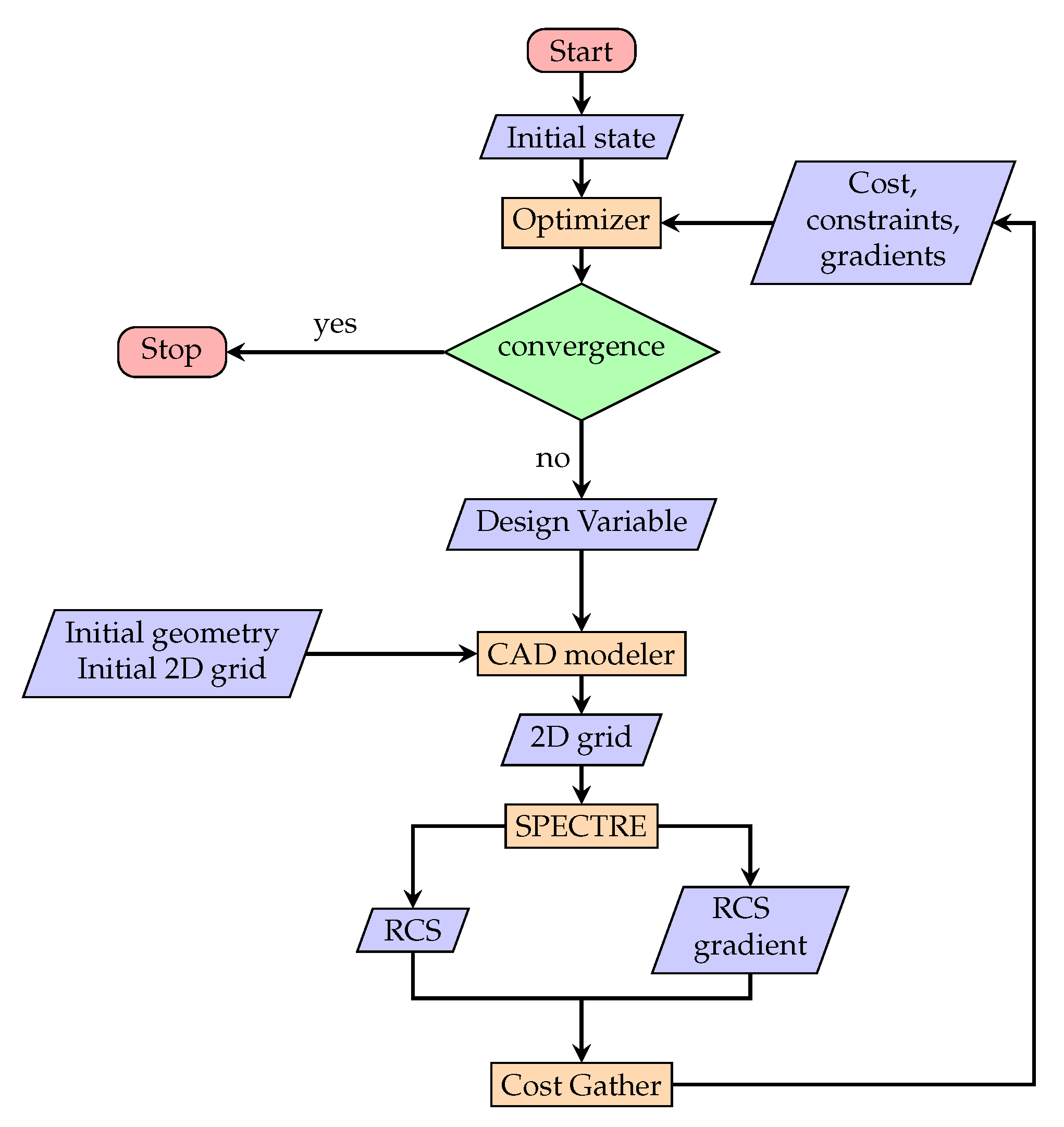
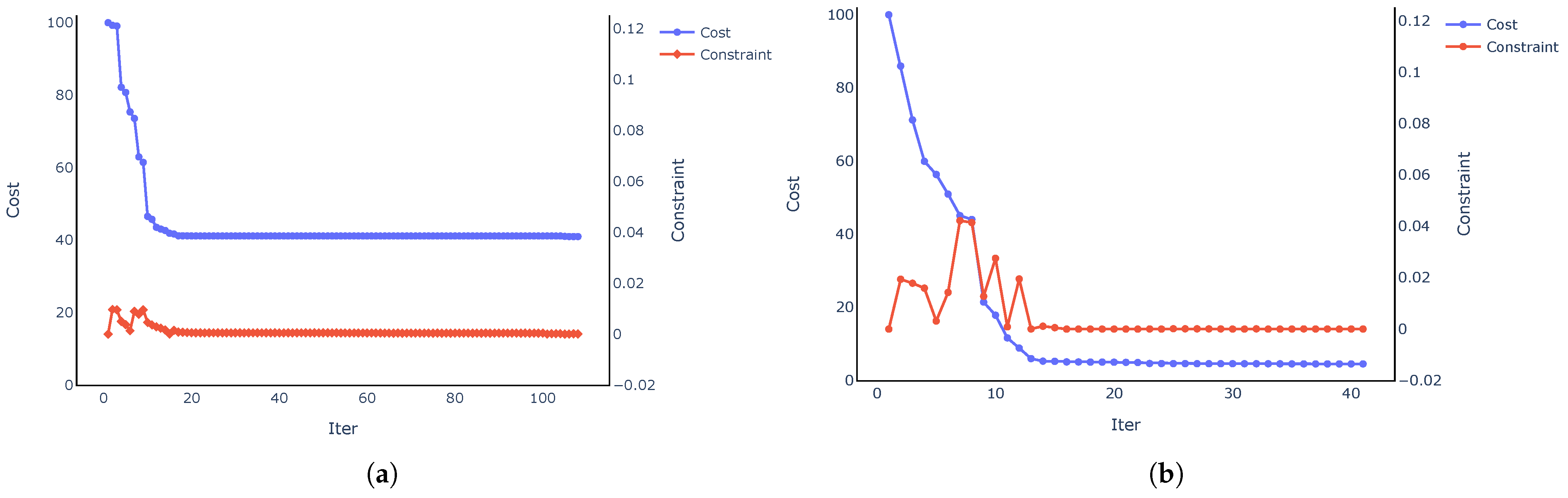
3.3. Optimization Process and Algorithm

The flowchart of the gradient-based optimization process is presented in Figure 3. The optimization algorithm involves Sequential Least Squares Quadratic Programming (SLSQP) [29], which allows for constrained optimization problems.

First, an initial vector of the design variables, as well as an initial CAD geometry and a corresponding 2D grid, is given to the CAD modeler (presented in Section 3.1), which transforms the CAD geometry according to the design variable values, projects the 2D mesh onto the deformed geometry, and computes the gradient of the mesh displacement with respect to the design variables if needed. The 2D grid is then fed to the CEM solver (see Section 3.2 for more details), which computes the RCS and its gradient, if applicable. A post-processing script (Cost-Gather) takes the RCS, its gradient, and the interest functions computed by GANIMEDE in order to compute the objective function as well as the constraints and their gradient. Finally, the SLSQP algorithm decides if the process has converged or computes the next values of the design variables.

4. Validation

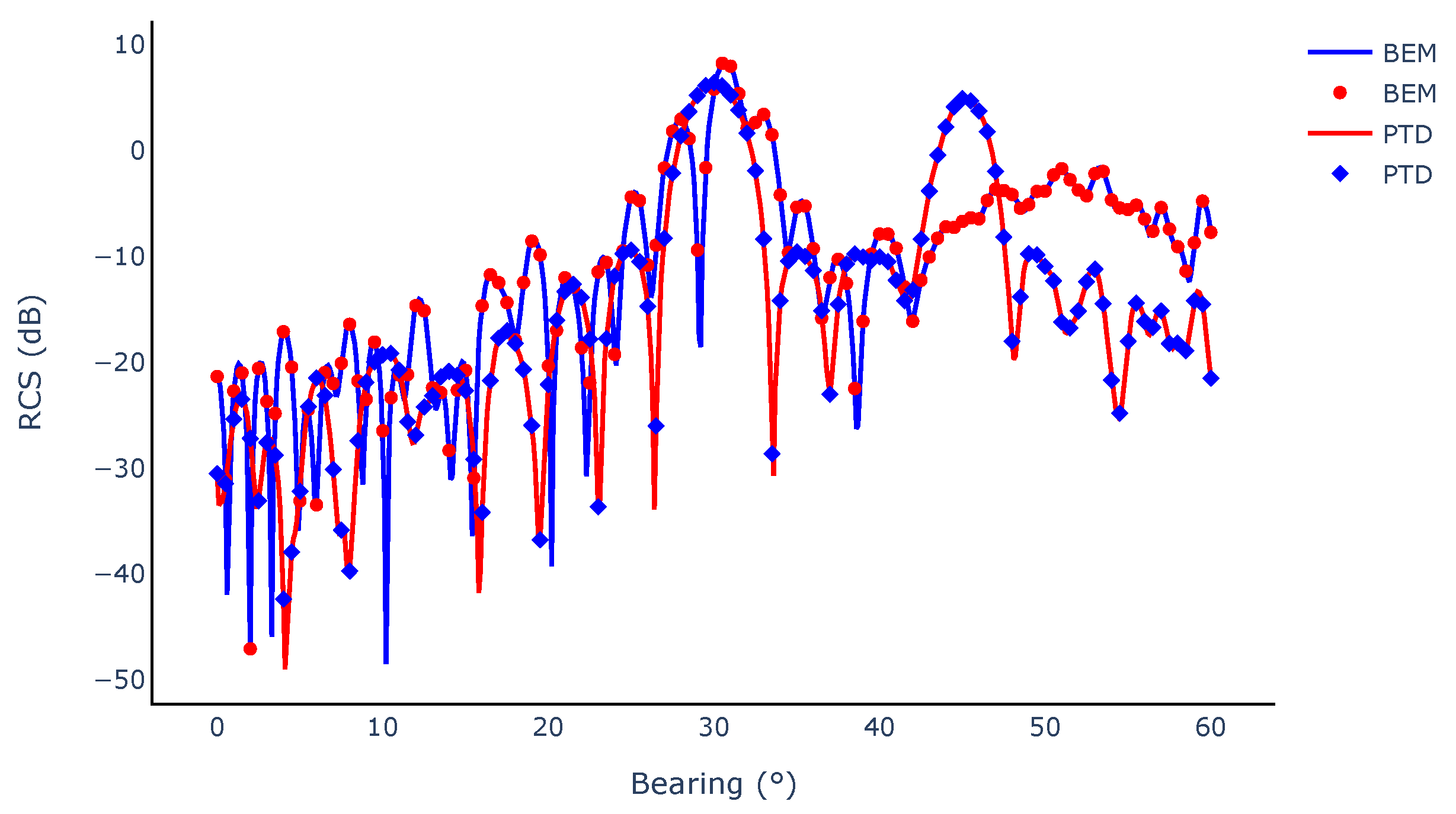
4.1. Validation of the BEM Solver

In order to validate the BEM computation, we used a sphere geometry as a test case. According to Mie’s theory, if a sphere of radius R is illuminated by a wave of wavelength $\lambda$, then the RCS $\sigma$ converges to the section area of the sphere as the wavelength decreases:

$$\underset{\lambda \to 0}{lim}\sigma =\pi R^2.$$

Moreover, due to the symmetric properties of the sphere, its RCS does not depend on the bearing angle.

Consider the quantity

$$F_s\left(R\right)={\left(\sigma \left(R\right)-\sigma \left(0.8\mathrm{m}\right)\right)}^2$$

(41)

Figure 4 shows $F_s\left(R\right)$ (see Equation (41)) computed using the BEM solver and its analytical value according to Mie’s theory for various values of R. The incident wave has a frequency of $2\mathrm{GHz}$, and the baseline sphere ($R=1\mathrm{m}$) is discretized with a step size of $15\mathrm{m}\mathrm{m}$. The figure shows good accordance.

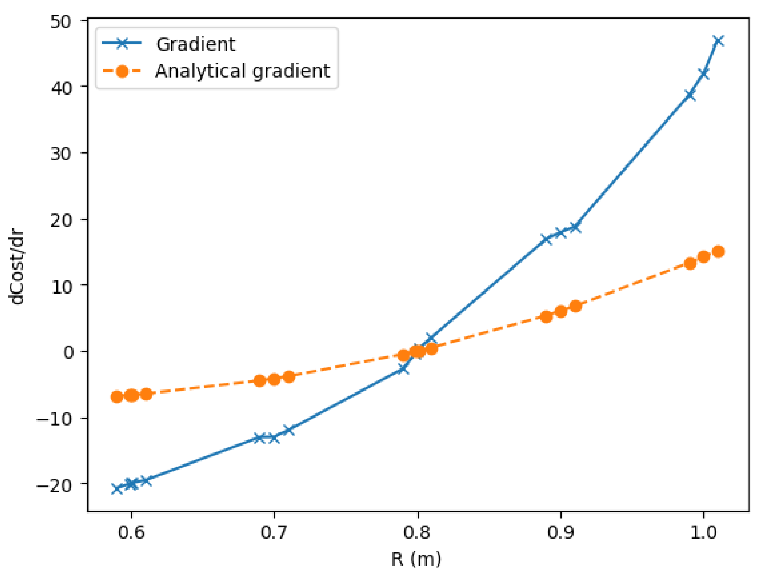
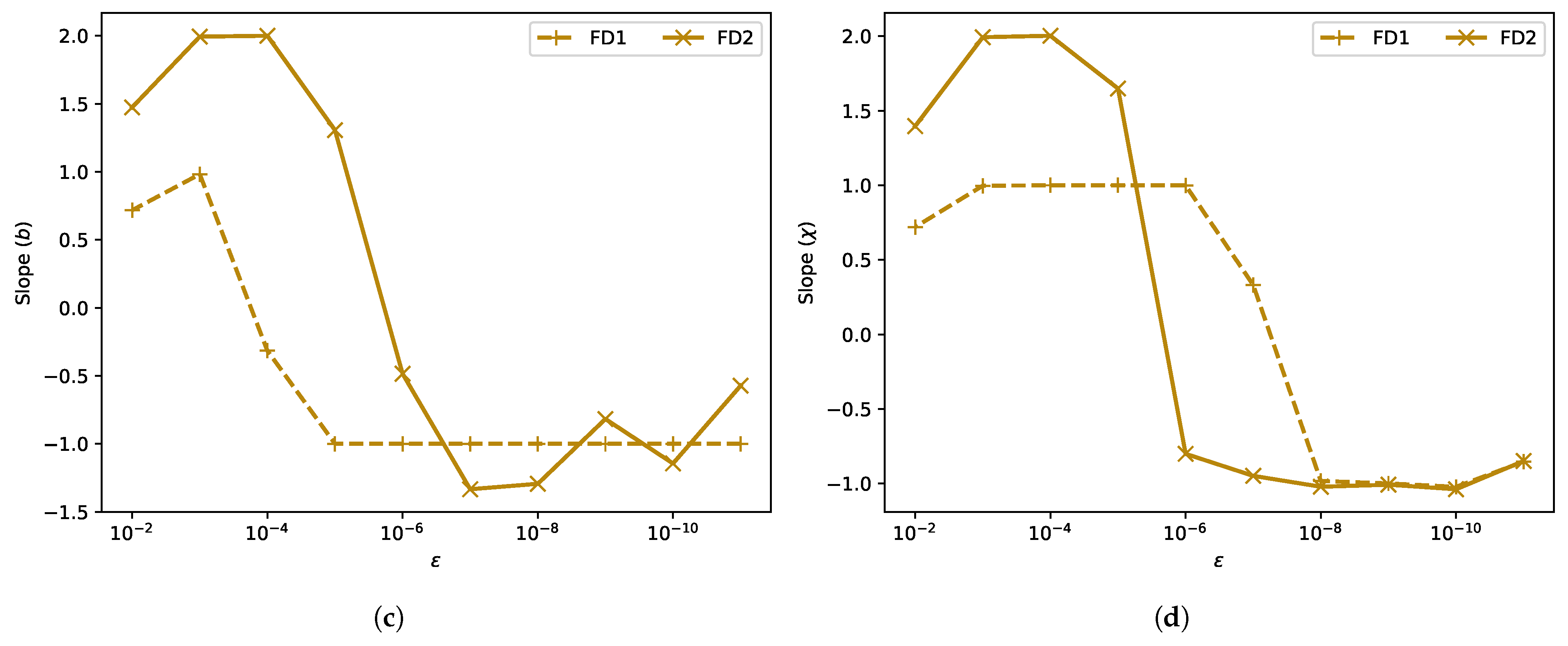
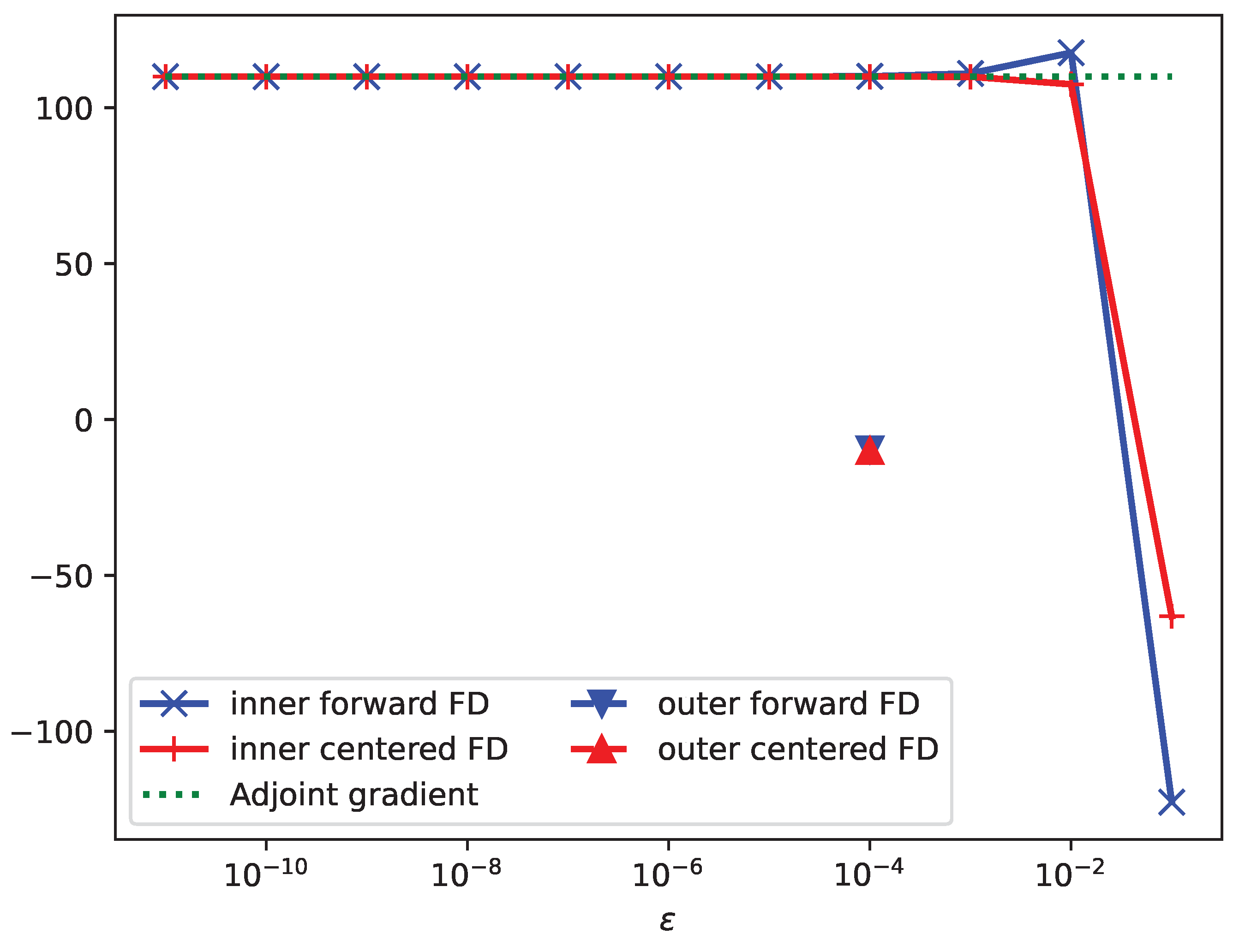
4.2. Validation of the Adjoint Gradients

Figure 5 shows the gradient $F_s^{\prime }\left(R\right)$ computed using the BEM solver and its analytical value according to Mie’s theory for various values of R.

The gradient computed by the BEM solver is not in agreement with the analytical value. Finer analysis is required in order to determine whether the gradient is wrong or whether the error is due to neglecting the term ${\displaystyle \frac{\partial A}{\partial X}}I$ in Equation (33).

If the gradient is properly computed, we expect that if the step size is small enough, the error decreases with the step size, up until a point where the numerical error on the function is of the same order of magnitude as the difference between the values of the RCS function at $\nu$ and $\nu +ϵ\widehat{d}$ (where $\widehat{d}$ is an arbitrary direction unit vector). After this critical point, the error should increase roughly linearly as the step size continues decreasing.

Let f denote a real-valued function, at least three times differentiable, with $f^{\prime }$ as its derivative and ${\Delta }_{ϵ}f$ and ${\delta }_{ϵ}f$ as its approximation with, respectively, the forward and centered Finite Difference (FD) with a step size of $ϵ$. It is well known that

$$\begin{array}{cc}\hfill {\Delta }_{ϵ}f-f^{\prime }=o\left(ϵ\right)& \mathrm{as}ϵ\to 0,\hfill \end{array}$$

(42)

$$\begin{array}{cc}\hfill {\delta }_{ϵ}f-f^{\prime }=o\left({ϵ}^2\right)& \mathrm{as}ϵ\to 0.\hfill \end{array}$$

(43)

Hence, the logarithm of the error between the exact gradient and the FD should be linear with respect to the step size if the step size is small enough but bigger than the critical step size, and its slope should be 1 for forward FD and 2 for centered FD. We consider that the minimal error should be at most ${10}^{-3}$ for forward FD and ${10}^{-6}$ for centered FD in order to deem the gradient acceptable.

Figure 6a,b show the norm of the difference between the gradient of the right-hand side and the RCS, respectively, with respect to the mesh coordinates computed by the SPECTRE solver and the FD gradient function of the FD step size, for both forward (dashed line) and centered (solid line) differences. These correspond to the terms ${\displaystyle \frac{\partial \zeta }{\partial b}}{\displaystyle \frac{\partial X}{\partial \nu }}$ and ${\displaystyle \frac{\partial \chi }{\partial X}}{\displaystyle \frac{\partial X}{\partial \nu }}$, respectively, in Equation (33).

Figure 6c,d show the evolution of the slope of the logarithm of the difference between the adjoint gradient and the FD gradients as a function of the FD step size.

Both terms show the expected behavior, which indicates that the gradient is properly computed.

Figure 7 shows the comparison between the adjoint gradient and the finite differences computed using two different methods. The inner finite-difference gradient is computed by computing the terms ${\displaystyle \frac{\partial \zeta }{\partial X}}{\displaystyle \frac{\partial X}{\partial \nu }}$ and ${\displaystyle \frac{\partial b}{\partial X}}{\displaystyle \frac{\partial X}{\partial \nu }}$ with finite differences and computing the gradient using expression (33). The outer finite-difference gradient is derived by computing the finite difference of $\sigma$ with respect to a small variation in $\nu$.

The gradient is in very good accordance with the inner finite differences, but it does not correspond at all of the outer finite differences. This indicates that the error on the gradient observed in Figure 5 is entirely due to neglecting the term ${\displaystyle \frac{\partial A}{\partial X}}I$.

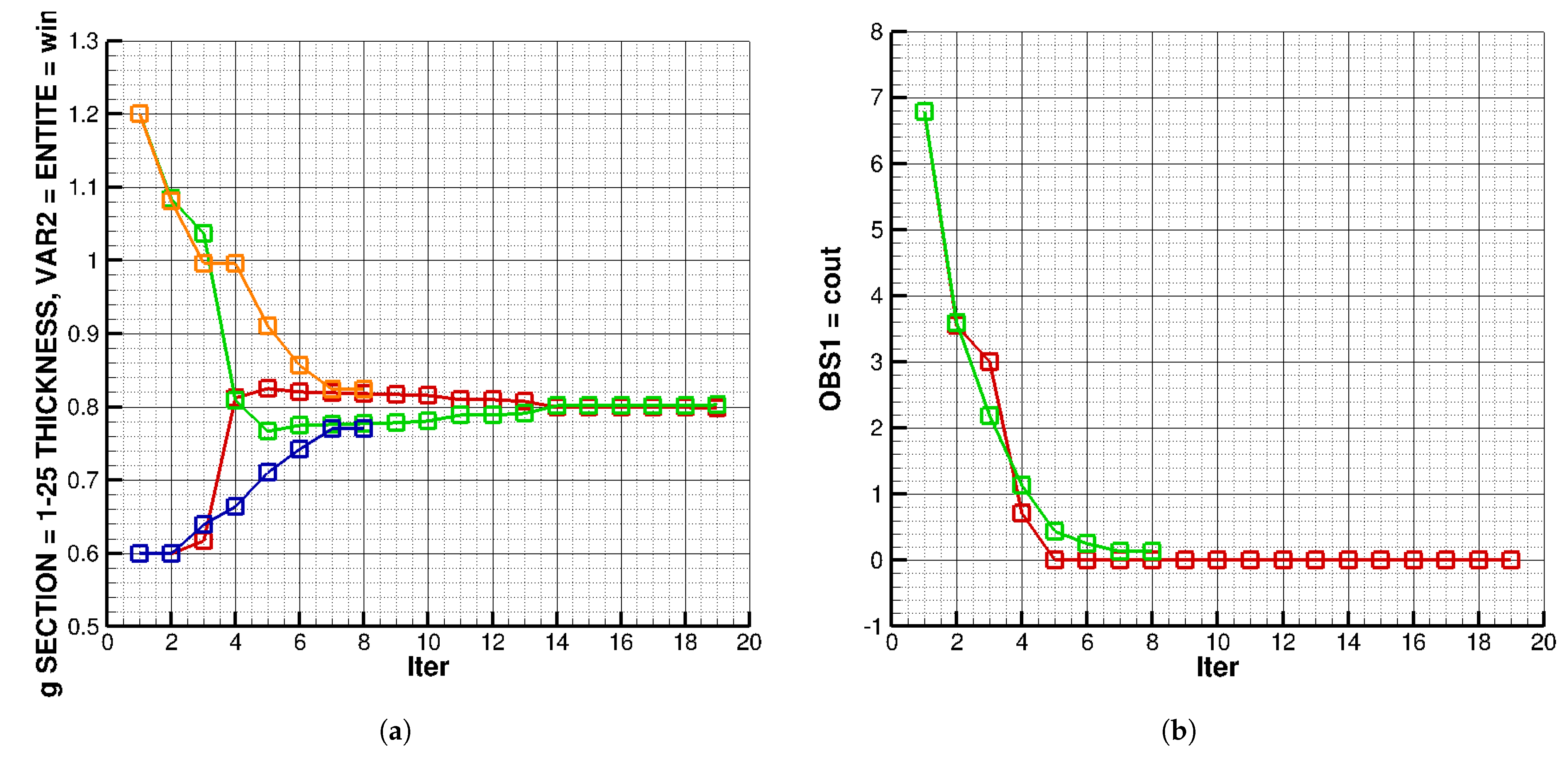
4.3. Ellipsoid Optimization (Two Variables)

In order to validate the solver, we first performed an optimization of an ellipsoid with two parameters. Because GANIMEDE is designed to primarily handle aircraft geometries, it is not really adapted to the manipulation of a geometry such as an ellipsoid. For this reason, we were not able to find a parametrization akin to the main and secondary radii, and no intuitive couple of design variables were able to transform a 1 $\mathrm{m}$ sphere into a 0.8 $\mathrm{m}$ ellipsoid. Because of the symmetries, it is not necessary to observe the shape from every direction. Only three observation directions are enough, as long as they are not coplanar. The cost function is the quadratic error between the RCS of the shape and that of the target:

$$F_e({\nu }_1,{\nu }_2)=\sum _{i=1}^4{\left({\sigma }_{{\theta }_i}({\nu }_1,{\nu }_2)-{\sigma }_{{\theta }_i}^{\mathrm{target}}\right)}^2.$$

(44)

The results of the optimization are shown in Figure 8. We compare them to two other optimizations on the same test case. In one, the gradient is computed via outer finite differences. In the other one, we used a PO solver (see Section 5.1.2) in order to evaluate the RCS.

5. Aircraft Shape Optimization

5.1. Case Presentation

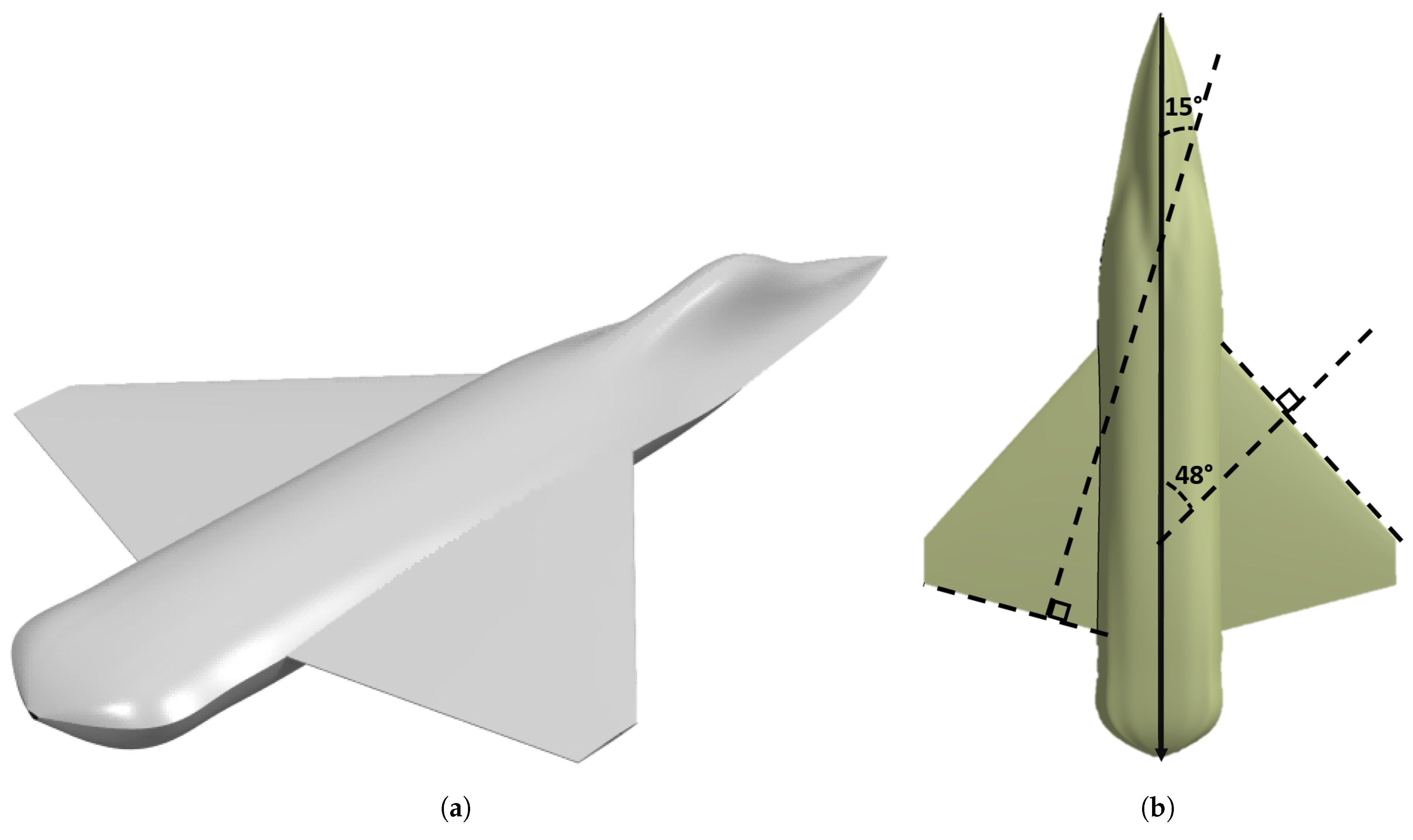
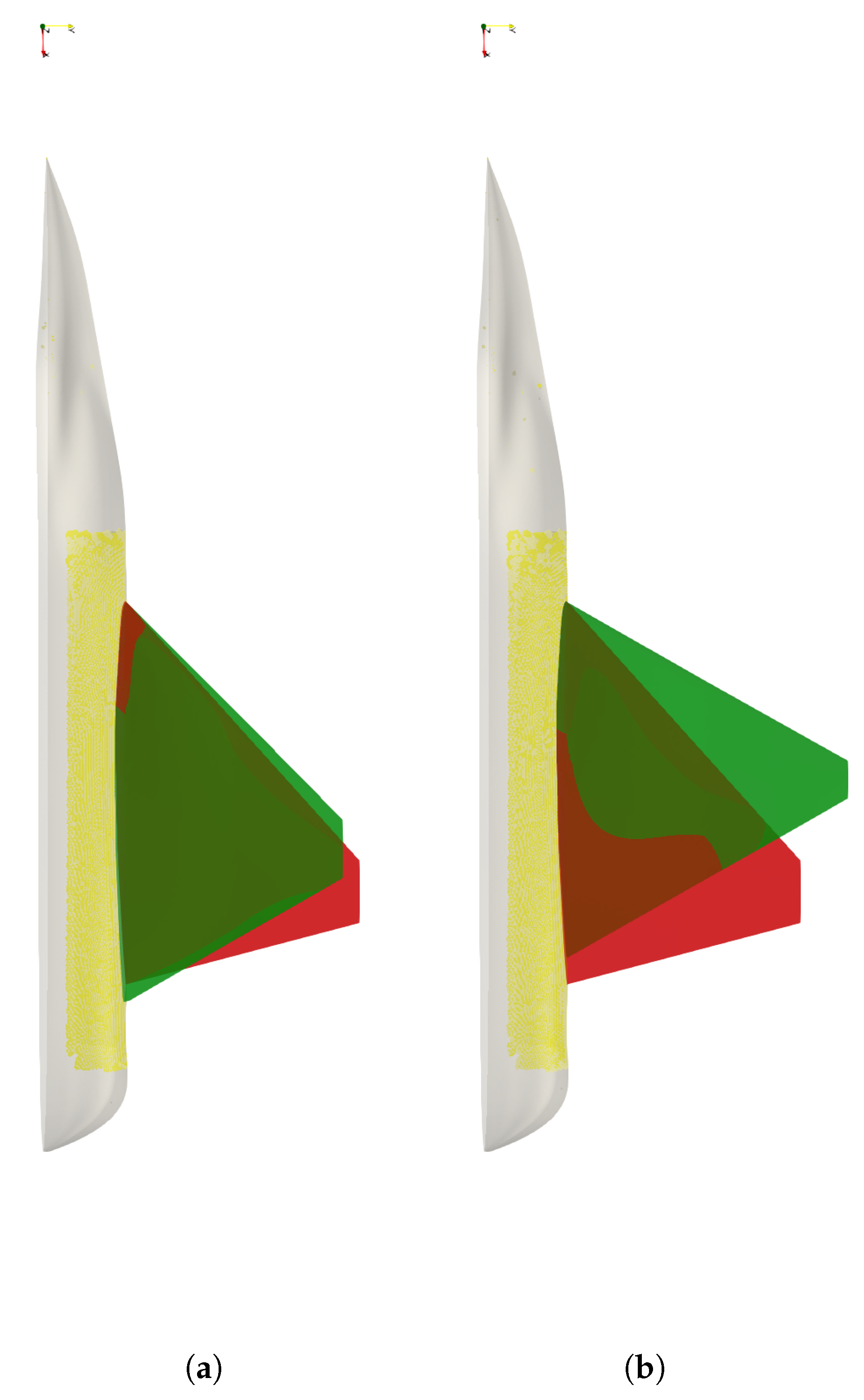
5.1.1. Baseline Description

The geometry we used is a simplified shape of a Generic Fighter Aircraft (GFA; see Figure 9). It features the fuselage without air intake and a pair of wings. The wings have a trapezoidal shape, without leading edge extension. It does not have a tail fin, horizontal stabilizer, or canard. The front of the fuselage has a ridge on both side. We did not use a realistic geometry for the rear of the fuselage, so the physics of the wake will not be accurately represented. Since we only performed supersonic simulations, this will not disturb the flow upstream. This also allowed us to be lenient with meshing the downstream region, thus saving computation time.

5.1.2. Stealth Analysis of the Baseline

In order to analyze the baseline RCS profile, we performed a simulation with an in-house approximate solver using the Physical Optics (PO) method, described in a previous work [2] and called COPOLA.

The COPOLA simulation was carried out on a range of bearing angles from 0 to ${70}^{°}$ with a step of ${0.01}^{°}$ and for an elevation angle of $-{10}^{°}$ in order to simulate an aircraft reflecting hostile waves from a radar on the ground far in front of the plane. For each line of sight, the simulation was run for five frequencies around a main frequency at $500\mathrm{MHz}$ and spanning $100\mathrm{MHz}$. The step for the bearing was chosen according to the Shannon criterion.

In Figure 10a,b, a peak is visible around ${48}^{°}$ of bearing. This corresponds to the direction the leading edge is facing. This peak is the specular reflection of the incident wave onto the leading edge. With the vertical polarization, in Figure 10a, a second peak appears at around 15°. This peak has a lower intensity compared to the specular reflection peak. This is due to the non-continuity of the normal at the trailing edge wedges. Physically, this means that the trailing edge wedges diffract the incident wave. However, the peak is almost absent with the horizontal polarization in Figure 10b. This is because of the horizontality of the trailing edges [30].

Over the rest of the observation window, the RCS is very low, around $-30$ to $-20$ dB, which is practically negligible, but increases as the bearing angle comes close to ${70}^{°}$. This is likely due to the influence of the fuselage, but as it is far away from the axis of the plane, it is not relevant to this study. One might note however that the value around ${70}^{°}$ is not the same with or without the PTD extension. This is likely due to a diffraction by the wing tip of by wedges on the fuselage that are overestimated by PO alone.

Since the vertical polarization is strictly richer than the horizontal polarization in our case, it is the one we will be using for RCS simulation in the rest of this study.

Figure 11 compares the RCS of the baseline computed with the PTD solver and the BEM solver. The PTD tends to underestimate the RCS away from the specular reflection (${30}^{°}$) or the wedge diffraction (${15}^{°}$) peaks, as it neglects most forms of diffraction. The PTD RCS also tends to be smoother than the BEM RCS. Therefore, the BEM RCS may be more dependant on a small shape variation, and the BEM optimization may struggle to converge compared to PTD optimization. In order to mitigate this effect, we could consider computing over a narrow range of frequencies and using the average RCS instead.

5.2. Optimization Parameters

The wing of the GFA is parameterized with the help of six control sections, with 15 control points along each of them (see Figure 12). All sections are parallel and remain parallel to the symmetry plane. Section S1 is at the symmetry plane and will not be modified. Section S2 is a few centimeters away from the root of the wing. At Section 4, the continuity of the tangent is not ensured, allowing for a sharp angle on the wing. The fuselage is not modified.

The geometry is parameterized with the help of 13 global variables:

• The leading edge sweep angle of sections S2 and S4;
• The chord of sections S2, S4, and S6;
• The distance between sections S2 and S6;
• The twist angle of sections S2, S3, S5, and S6,
• The leading edge camber of sections S3, S5, and S6.

The chords of sections S3 and S5 are interpolated between those of sections S2 and S4 and S6, respectively. The twist angle for a given section is a rotation along an axis perpendicular to the section going through a point at 25% chord and 50% thickness. Both the leading edge camber and the twist angle at section S4 are interpolated between sections S3 and S5.

5.3. Cost and Constraints

5.3.1. Criterion

We used two distinct criteria.

Average over the Observation Window

This criterion is the simpler one. It is defined as

$$F_e^a={\displaystyle \frac{{\tilde{\sigma }}_a}{{\tilde{\sigma }}_a^{ref}}},$$

(45)

where ${\tilde{\sigma }}_a$ is the average of the RCS $\sigma$ over the observation window.

$${\tilde{\sigma }}_a={\int }_{{\theta }_0}^{{\theta }_1}{\int }_{{\varphi }_0}^{{\varphi }_1}\sigma sin\left(\varphi \right)\mathrm{d}\theta \mathrm{d}\varphi .$$

(46)

Peak Directions

Typically, a stealth aircraft shape is designed to scatter radar wave away from any hostile radar antenna, which is usually located roughly in front of the aircraft, slightly below. For example, the upward-facing planes of the Lockheed Martin F-117 scatter the radar wave into the sky, while more modern aircraft, like the Northtrop B-2, are built to concentrate the reflected radar wave only as a very narrow signal in a few specific directions (“peak directions”). The stealth criterion was built to reflect and favor this behavior: the goal is to minimize the RCS in every direction in a given sector $({\theta }_0,{\theta }_1)\times ({\varphi }_0,{\varphi }_1)$, except for a limited interval around a peak direction where the RCS can be high.

In order to manage dimensionless quantities, the electromagnetic criterion is defined as follows:

$$F_e^f={\displaystyle \frac{{\tilde{\sigma }}_f}{{\tilde{\sigma }}_f^{ref}}},$$

(47)

where ${\tilde{\sigma }}_f$ is a weighed average of a function of ${\sigma }_{\mathrm{dB}}$:

$${\tilde{\sigma }}_f={\int }_{{\theta }_0}^{{\theta }_1}{\int }_{{\varphi }_0}^{{\varphi }_1}{\Gamma }_d\left(\theta \right){\delta }_s\left({\sigma }_{\mathrm{dB}}\right)sin\left(\varphi \right)\mathrm{d}\theta \mathrm{d}\varphi .$$

(48)

Function ${\delta }_s$ is a differentiable threshold function built to cut the low-intensity variations that have a negative impact on the computation of the gradient of the cost function:

$${\delta }_s\left(x\right)={\displaystyle \frac{x-s}{1+e^{-\mathit{\tau }(x-s)}}},$$

(49)

with $\tau$ as a parameter that allows us to control the sharpness of the peak. The threshold $s=-5\mathrm{dB}$ was chosen.

Function ${\Gamma }_d$ is a weighting function chosen to favor the peak directions. It is close to 1 everywhere, except in the neighborhood of direction d where it decreases quickly:

$${\Gamma }_d\left(\theta \right)=1-{\displaystyle \frac{1}{2}}\sum _{i=0}^4{\displaystyle \frac{6-i}{10}}exp\left(-{\left({\displaystyle \frac{\theta -d}{{10}^i\mathit{\tau }}}\right)}^2\right).$$

(50)

Graphs of function ${\Gamma }_d$ are shown in Figure 13 for various values of $\tau$. For this study, we chose, somewhat arbitrarily, a peak direction at a bearing of $d={30}^{°}$ and $\tau =0.1$.

In both cases, in order to smooth the dependence of the RCS over the shape of the target and improve the optimization convergence, the criterion may be averaged over multiple frequencies over a narrow band around the main frequency.

5.3.2. Constraints

In order to prevent the optimizer from generating an unrealistic shape, we want to preserve the reference surface (${\mathrm{S}}_{\mathrm{ref}}$) of the wing. ${\mathrm{S}}_{\mathrm{ref}}$ is defined in Figure 14.

5.4. Results

An optimization was performed using the the criterion $F_e^f$ (defined in Equation (47)). Due to time constraints, only one frequency was used ($f=500\mathrm{MHz}$). In the following section, the results of this optimization are presented and compared to two reference optimizations: one using the BEM solver but computing an approximate gradient using centered finite differences, and another using the exact gradient PTD solver presented in [2].

The adjoint optimization was able to converge in a few iterations (Figure 15a), though not as precisely as with the finite differences (see Figure 15b): the FD optimization was able to reduce the cost function by around 80%, while the adjoint optimization only improved the cost by around 40%. This difference is probably due to the missing term in the BEM adjoint. In contrast, the constraint was better resolved by the adjoint computation than the finite differences, with an error on the constraint of $1\times {10}^{-6}$ for the adjoint optimization and $1\times {10}^{-3}$ for the FD optimization. The adjoint optimization converged in fewer iterations than that with finite differences.

The shape of the adjoint and FD optimization (Figure 16), as well as their RCS signature (Figure 17), are quite different from each other, as can be expected from the difference in cost values at the end of the optimization. As expected, the direction of ${30}^{°}$ is favored by the optimizer no matter the method. This is due to the chosen cost function; see Section 5.3.1. Physically, this is mainly achieved by manipulating the sweep angles so that both the leading and trailing edges of the wings tend to face the ${30}^{°}$ direction.

The adjoint optimization tried to modify the leading edge sweep angles (as seen in Figure 16a) towards the peak direction, but it did not quite succeed (see Figure 17a). The specular peak is also less intense than would be expected when looking only at the platform. The presence of a sharp angle on the middle of the leading edge might explain it: the same quantity of energy is now distributed between two directions, and some diffraction phenomena may take place along the wedge or corners. On the other hand, the trailing edge sweep angles were modified so that the EM wave is reflected outside of the observation window.

The FD optimization brought the leading edge sweep angle and the tip section trailing edge sweep angle closer to ${30}^{°}$ (see Figure 16b and Figure 17b), which aligned the specular and diffraction peaks close to the cut direction of ${30}^{°}$. Similarly to the BEM adjoint, the root section of the trailing edge was modified so that the wave is diffracted outside of the observation window. This is a valid way of reducing the RCS in the observation window, though it is not the behavior that was expected.

In contrast, the PTD optimization converged better than the adjoint BEM, but not as well as the FD BEM (Figure 15c). The trailing edge sweep angle is at ${30}^{°}$ (see Figure 16c and Figure 17c), but the leading edge sweep angle barely moved at all. The fact that the PTD optimization, whose gradient is exact and has been validated, struggled to converge suggests that the missing term in the adjoint is not the only factor responsible for the poor convergence of the BEM adjoint optimization.

Figure 18 shows the results of a BEM computation on the optimum found through the PTD optimization. First, it can be noted that the PTD RCS is once again smoother than the BEM RCS, which could explain why the BEM optimizations struggle to converge, especially as the shapes become more complex. Second, the specular peak at around ${45}^{°}$ is much wider and less intense in the BEM than PTD. This would be detrimental to the criterion and means that the optimal form computed with PTD might not be as good when computed using the BEM. The flattening of the specular peak with what can be seen of the RCS of the other optimal shapes (Figure 17a,b) may result from interactions between the wing and the fuselage, or from diffraction phenomena that are not captured by the PTD solver. This suggests that a PTD optimization alone may not be enough to design a true stealth shape and that the BEM optimization may be necessary.

When the optimization criterion is averaged over a $100\mathrm{MHz}$ wide band centered on the main frequency ($500\mathrm{MHz}$) with a step of $50\mathrm{MHz}$, the convergence of the PTD optimization is improved dramatically, as can be seen in Figure 19, where the cost almost reached 0 and in far fewer iterations (Figure 19b) than for the optimization with only one frequency (Figure 19a). This is because the frequency average tends to make the RCS less sensitive to a small shape variation.

Figure 20b shows that the multifrequency optimization was able to produce the intended shape with both the leading edge and the trailing edge aligned with an angle of $\pm {30}^{°}$, which translates in both the specular reflection and the wedge diffraction peaks (respectively, at ${48}^{°}$ and ${15}^{°}$ on the baseline RCS; see Section 5.1.2 for more details) being superimposed (Figure 21b) at ${30}^{°}$, thus greatly reducing the observability in the rest of the observation window.

This suggests that, more than the missing term of the BEM adjoint, averaging the criteria over a narrow band of frequencies could smooth the evolution of the criterion with respect to the shape parameters and improve the convergence.

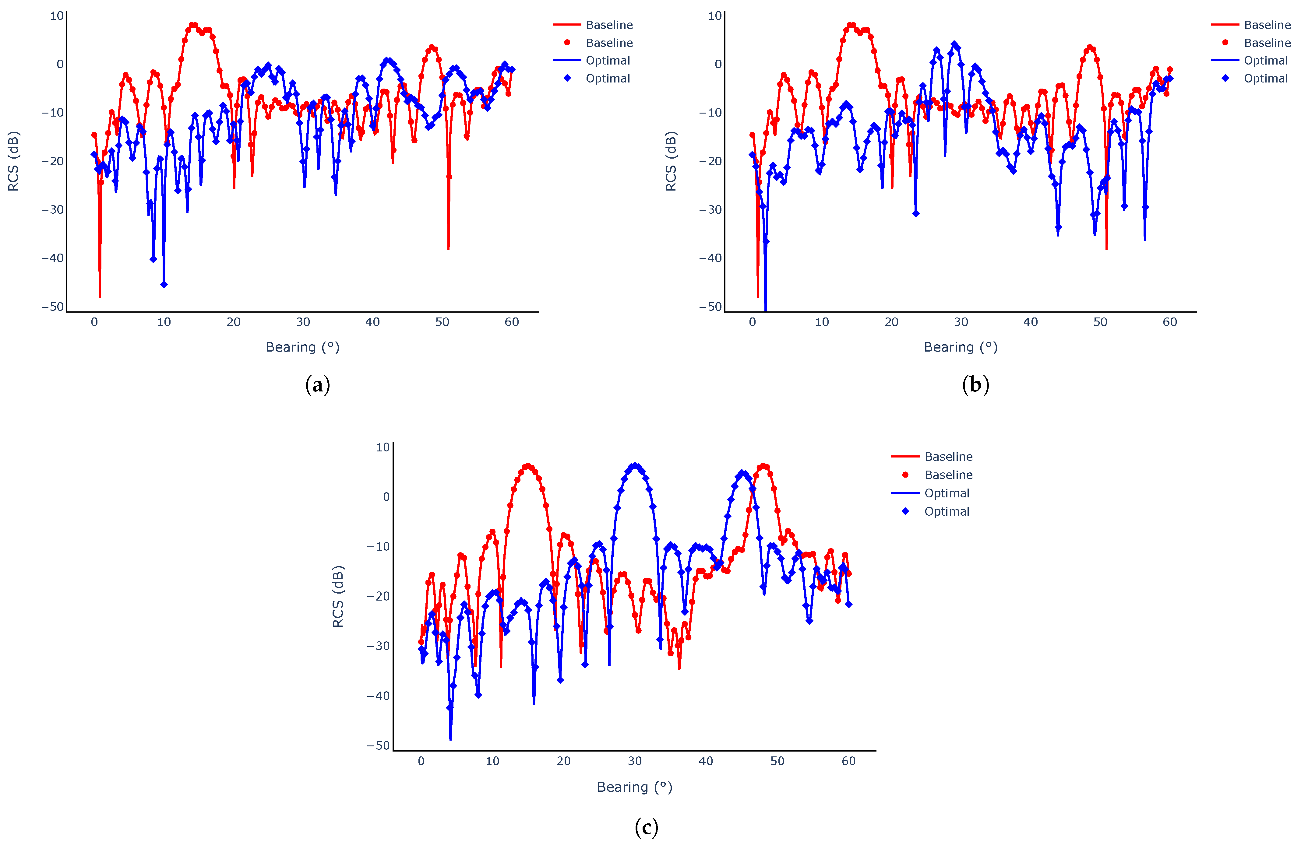
The computation time of the adjoint is around 2 h, whereas the computation time for the computation of the primal problem is around 15 min. Thus, it is more efficient to use the adjoint formulation starting from eight design variables.

6. Conclusions

In this paper, we presented an adjoint formulation for the BEM in order to perform high-fidelity gradient-based RCS shape optimization for an aircraft. We differentiated our in-house BEM solver with the AD tool TAPENADE in order to implement it. Because of time constraints, we did not have time to implement one of the terms of the adjoint, but we have shown that the gradient is still accurate enough to perform a monodisciplinary optimization. We validated the RCS gradient with respect to shape parameters for various shapes. We then showcased our formulation on a simplified aircraft shape with 13 design variables. With this number of variables, the adjoint optimization is much more efficient than the finite difference optimization from a computation time standpoint, though the adjoint computation would benefit from further optimization in order to reach maximum efficiency.

The missing term in the adjoint means that the optimization is not as precise as it could be, but the time gained with respect to the finite difference makes it preferable in an industrial framework despite the loss in accuracy. We did not compute it due to technical and time constraints, but it will be computed in a subsequent study. The main difficulty in computing the missing term is the storage requirements of ${\displaystyle \frac{\mathrm{d}A}{\mathrm{d}X}}$, which is in $\mathcal{O}\left(N^2\right)$, with N as the number of unknowns, for each design variable. This is not feasible in a realistic industrial application. This means that simply using the TAPENADE to differentiate the routines building the matrix as we did for the other terms is not practical. The solution is to exploit the current behavior of the routine building matrix A, that is, to build the matrix block by block and then assemble it. With this, we will differentiate only the block-building routine, multiply the block of the differentiated matrix by the corresponding block of vector I, and then assemble vector ${\displaystyle \frac{\mathrm{d}A}{\mathrm{d}X}}$. However, even with this incorrect gradient, the optimizer was able to reduce the cost while satisfying the constraint. Therefore, taking into account the gain in computational cost, even this preliminary version of the adjoint has use in an industrial framework. Moreover, the monofrequency vs. multifrequency PTD study that we performed seems to suggest that the worse convergence of the BEM adjoint optimization may be explained to some extent by the fact that the computation was carried out with only one frequency.

The BEM computation that we performed on the PTD optimal shape seems to suggest that important phenomena are not captured by the PTD solver, which may play a role in stealth optimization. As such, the added fidelity of the BEM optimization may be necessary for a satisfactory result, especially when more subtle effects than the impact of wing sweep angles are investigated. Moreover, though it was not featured in this study, PTD is inherently unable to handle cases such as multi-reflection or, more importantly, cavities, which is essential to compute the RCS contribution of air intakes. Due to the comparatively higher cost of BEM optimization, hybrid PTD-BEM frameworks should be investigated. The most obvious option would be a framework where PTD optimization is first performed to produce a first optimal shape, which is then used as the starting point of BEM optimization, which hopefully would then need fewer iterations to converge to a better shape. On the other hand, Jakobus and Landstorfer made significant contributions to the hybrid approaches using BEM and PO methods [31,32], which could also be beneficial in a more efficient RCS optimization framework.

The fact that the monofrequency PTD optimization did not manage to converge to the expected shape when the multifrequency PTD optimization did suggests that a multifrequency BEM computation is also required for the BEM optimization to converge to a satisfactory result. However, it was not feasible with realistic time constraints, as the computation time of both the primal and adjoint problems is proportional to the number of frequencies used, and even averaging over a dozen frequencies would have made the computation prohibitively expensive. As such, acceleration methods such as ACA, H-matrix, or a fast multipole method need to be used for further studies.

References

- Knott, E.F.; Schaeffer, J.F.; Tulley, M.T. Radar Cross Section; SciTech Publishing: New York, NY, USA, 2004. [Google Scholar]
- Thoulon, C.; Roge, G.; Pironneau, O. Gradient-Based Aero-Stealth Optimization of a Simplified Aircraft. Fluids 2024, 9, 174. [Google Scholar] [CrossRef]
- Parr, J.; Holden, C.M.; Forrester, A.I.; Keane, A.J. Review of Efficient Surrogate Infill Sampling Criteria with Constraint Handling. 2010. Available online: https://eprints.soton.ac.uk/336169/ (accessed on 28 April 2025).
- Lyu, Z.; Xu, Z.; Martins, J. Benchmarking optimization algorithms for wing aerodynamic design optimization. In Proceedings of the 8th International Conference on Computational Fluid Dynamics, Chengdu, China, 14–18 July 2014; Volume 11, p. 585. [Google Scholar]
- Martin, L. Conception Aérodynamique Robuste. Ph.D. Thesis, Université de Toulouse, Université Toulouse III-Paul Sabatier, Toulouse, France, 2010. [Google Scholar]
- Hascoët, L.; Pascual, V. The Tapenade Automatic Differentiation tool: Principles, Model, and Specification. ACM Trans. Math. Softw. 2013, 39, 1–43. [Google Scholar] [CrossRef]
- Davidson, D.B. Computational Electromagnetics for RF and Microwave Engineering. In Chapter 1: An Overview of Computational Electromagnetics; Cambridge University Press: Cambridge, UK, 2010; pp. 1–10. [Google Scholar]
- Bardos, C.; Roge, G. Maîtrise du champ rétrodiffusé par une méthode de contrôle optimal. In Proceedings of the Séminaire de l’École Normale Supérieure, Paris, France, 20 January 1995. [Google Scholar]
- Lions, J.L.; Lelong, P. Contrôle Optimal de Systèmes Gouvernés par des Équations aux Dérivées Partielles. 1968. Available online: https://cir.nii.ac.jp/crid/1130000795441759872 (accessed on 28 April 2025).
- Paoli, J. Contrôle Optimal du Champ Rétrodiffusé et Optimisation Sous Contraintes. PhD. Thesis, Cachan, Ecole Normale Supérieure, Gif-sur-Yvette, France, 2001. [Google Scholar]
- Roge, G. Quelques applications de la Théorie du Contrôle de Jacques-Louis Lions chez Dassault Aviation. In Proceedings of the Journée Calcul Scientifique et Applications Technologiques, Paris, France, 27 November 2003. [Google Scholar]
- Georgieva, N.K.; Glavic, S.; Bakr, M.H.; Bandler, J.W. Feasible adjoint sensitivity technique for EM design optimization. IEEE Trans. Microw. Theory Tech. 2002, 50, 2751–2758. [Google Scholar] [CrossRef]
- Nikolova, N.K.; Safian, R.; Soliman, E.A.; Bakr, M.H.; Bandler, J.W. Accelerated gradient based optimization using adjoint sensitivities. IEEE Trans. Antennas Propag. 2004, 52, 2147–2157. [Google Scholar] [CrossRef]
- Wang, L.; Anderson, W.K. Adjoint-based shape optimization for electromagnetic problems using discontinuous Galerkin methods. AIAA J. 2011, 49, 1302–1305. [Google Scholar] [CrossRef]
- Zhou, L.; Huang, J.; Gao, Z. Radar Cross Section Gradient Calculation Based on Adjoint Equation of Method of Moment. In Proceedings of the 2018 Asia-Pacific International Symposium on Aerospace Technology (APISAT 2018), Chengdu, China, 16–18 October 2018; Zhang, X., Ed.; Springer: Singapore, 2019; pp. 1427–1445. [Google Scholar]
- Cheng, S.; Wang, F.; Wu, G.; Zhang, C. A semi-analytical and boundary-type meshless method with adjoint variable formulation for acoustic design sensitivity analysis. Appl. Math. Lett. 2022, 131, 108068. [Google Scholar] [CrossRef]
- Lan, L.; Zhou, Z.; Liu, H.; Wei, X.; Wang, F. An ACA-BM-SBM for 2D acoustic sensitivity analysis. AIMS Math. 2024, 9, 1939–1958. [Google Scholar] [CrossRef]
- Liu, H.; Wang, F.; Cheng, S.; Qiu, L.; Gong, Y. Shape optimization of sound barriers using an isogeometric meshless method. Phys. Fluids 2024, 36, 027116. [Google Scholar] [CrossRef]
- Chen, W. Singular boundary method: A novel, simple, meshfree, boundary collocation numerical method. Chin. J. Solid Mech. 2009, 30, 592–599. [Google Scholar]
- Wei, X.; Sun, L. Singular boundary method for 3D time-harmonic electromagnetic scattering problems. Appl. Math. Model. 2019, 76, 617–631. [Google Scholar] [CrossRef]
- Bendali, A. Equations Intégrales en Électromagnétisme. Cours BEM INSA Toulouse. 2013. Available online: https://www.math.univ-toulouse.fr/~abendali/polyelec1314.pdf (accessed on 28 April 2025).
- Stratton, J.A.; Chu, L. Diffraction theory of electromagnetic waves. Phys. Rev. 1939, 56, 99. [Google Scholar] [CrossRef]
- Rao, S.; Wilton, D.; Glisson, A. Electromagnetic scattering by surfaces of arbitrary shape. IEEE Trans. Antennas Propag. 1982, 30, 409–418. [Google Scholar] [CrossRef]
- Kleinveld, S.; Rogé, G.; Daumas, L.; Dinh, Q. Differentiated parametric CAD used within the context of automatic aerodynamic design optimization. In Proceedings of the 12th AIAA/ISSMO Multidisciplinary Analysis and Optimization Conference, Victoria, BC, Canada, 10–12 September 2008; p. 5952. [Google Scholar]
- Shannon, C. Communication in the Presence of Noise. Proc. IRE 1949, 37, 10–21. [Google Scholar] [CrossRef]
- Poggio, A.J.; Miller, E.K. Integral Equation Solutions of Three-Dimensional Scattering Problems; MB Associate: San Ramon, CA, USA, 1970; Chapter 4; pp. 195–264. [Google Scholar]
- Carayol, Q. Développement et Analyse D’une Méthode Multipôle Multiniveau pour L’électromagnétisme. Ph.D. Thesis, Université Paris 6, Paris, France, 2002. Available online: https://theses.fr/2002PA066485 (accessed on 28 April 2025).
- Young, R.C. Application of a Floating Point Systems AP190L Array Processor to Finite Element Analysis; General Atomics: San Diego, CA, USA, 1982. [Google Scholar] [CrossRef]
- Nocedal, J.; Wright, S.J. Large-Scale Unconstrained Optimization; Springer: Boston, MA, USA, 2006; pp. 164–192. [Google Scholar]
- Jenn, D. Radar and Laser Cross Section Engineering; American Institute of Aeronautics and Astronautics, Inc.: Reston, VA, USA, 2005. [Google Scholar]
- Jakobus, U.; Landstorfer, F.M. Improved PO-MM hybrid formulation for scattering from three-dimensional perfectly conducting bodies of arbitrary shape. IEEE Trans. Antennas Propag. 2002, 43, 162–169. [Google Scholar] [CrossRef]
- Jakobus, U.; Landstorfer, F.M. Improvement of the PO-MoM hybrid method by accounting for effects of perfectly conducting wedges. IEEE Trans. Antennas Propag. 2002, 43, 1123–1129. [Google Scholar] [CrossRef]
Disclaimer/Publisher’s Note: The statements, opinions and data contained in all publications are solely those of the individual author(s) and contributor(s) and not of MDPI and/or the editor(s). MDPI and/or the editor(s) disclaim responsibility for any injury to people or property resulting from any ideas, methods, instructions or products referred to in the content. |
© 2025 by the authors. Licensee MDPI, Basel, Switzerland. This article is an open access article distributed under the terms and conditions of the Creative Commons Attribution (CC BY) license (https://creativecommons.org/licenses/by/4.0/).
Share and Cite
Thoulon, C.; Roge, G.; Pironneau, O. A BEM Adjoint-Based Differentiable Shape Optimization of a Stealth Aircraft. Eng 2025, 6, 147. https://doi.org/10.3390/eng6070147
Thoulon C, Roge G, Pironneau O. A BEM Adjoint-Based Differentiable Shape Optimization of a Stealth Aircraft. Eng. 2025; 6(7):147. https://doi.org/10.3390/eng6070147
Chicago/Turabian StyleThoulon, Charles, Gilbert Roge, and Olivier Pironneau. 2025. "A BEM Adjoint-Based Differentiable Shape Optimization of a Stealth Aircraft" Eng 6, no. 7: 147. https://doi.org/10.3390/eng6070147
APA StyleThoulon, C., Roge, G., & Pironneau, O. (2025). A BEM Adjoint-Based Differentiable Shape Optimization of a Stealth Aircraft. Eng, 6(7), 147. https://doi.org/10.3390/eng6070147