Research on the Reconstruction of the Temperature Field in Two-Dimensional Steady-State Thermal Conductivity Based on Physics-Informed Neural Networks

Abstract

This study investigates a simulation-based approach to the inverse problem of two-dimensional steady-state heat conduction in flat plates by employing Physics-Informed Neural Networks (PINNs). The primary objective is to reconstruct the temperature field and deduce unknown boundary conditions using limited labeled data sourced from conventional numerical methods. This work specifically validates the methodology using simulated data with known original conditions, rather than addressing truly unknown boundary conditions in real-world scenarios. By leveraging PINNs, the approach integrates physical laws with data-driven learning, facilitating the efficient inversion of boundary conditions and precise reconstruction of the temperature field. Within a temperature range of 10 °C to 40 °C, the method consistently achieves an average relative error of less than 10% and maintains an absolute error within 1 °C across the computational domain. By optimizing the distribution of sample points without increasing their quantity, the average relative error is further reduced by approximately 1%, thereby enhancing inversion accuracy. Additionally, implementing an adaptive weight adjustment strategy, based on learning rate annealing, further refines the method, reducing the maximum absolute error by 0.4 °C and the average relative error by 2% when compared to traditional PINNs. This research demonstrates the capability of PINNs to provide a rapid and effective solution for inverse heat conduction problems, establishing a foundation for their potential application in addressing complex inverse heat transfer challenges.

1. Introduction

The development of new techniques for solving inverse heat transfer problems (IHTPs) is a fundamental aspect of modern heat transfer. Many scientific and industrial applications involve physical processes that make it difficult or even impossible to directly measure the parameters involved. Alternatively, the inverse analysis in heat transfer involves reversing the classical direct (forward) problem by estimating the physical cause (such as a boundary heat flux, for example) using data describing the thermal effect (the temperature field of the investigated body) [1]. In many scientific and engineering fields, such as energy transmission, material processing, and the heat dissipation of electronic devices, it is of paramount importance to accurately understand the temperature distribution inside objects and the boundary thermal conditions. The inverse heat conduction problem aims to infer unknown boundary conditions, thermophysical parameters, or heat source distributions based on partially measurable information (such as limited temperature measurement data). The resulting solution results play an irreplaceable role in optimizing system design, ensuring the safe and stable operation of equipment, and improving energy utilization efficiency.

Partial differential equations (PDEs) are an important tool for representing the physical laws of heat transfer processes. The essence of IHTP can be explained as solving PDE with missing terms in heat transfer processes. The research methods of IHTP can be roughly divided into three categories during the development over the past few decades, namely the Tikhonov Regularization Method, gradient-based optimization algorithms, and gradient-free optimization algorithms. Glasko et al. [2] introduced the Tikhonov Regularization Method into the solution of IHTP and proposed a special regularization algorithm for the Neumann boundary condition of the nonlinear heat conduction equation. They also verified the accuracy of the results and the computational efficiency through numerical simulation. Artyukhin and Rumyantsev [3] used the Steepest Descent Method (SDM) to predict the boundary heat flux distribution of multi-dimensional heat transfer systems. Huang and Chen [4] focused on the boundary conditions of IHTP based on the Conjugate Gradient Method (CGM). Duda and Taler [5] determined the boundary conditions and temperature field of the water-cooled wall by combining the Levenberg–Marquardt (L-M) algorithm with experiments. Cortés et al. [6] inversely deduced the heat source temperature of the protective hot plate via the Particle Swarm Optimization (PSO) algorithm. Kim and Baek [7] inversely deduced the radiation coefficient of two-dimensional irregular geometries via the Genetic Algorithm (GA). Sablani [8] modeled the surface heat transfer coefficient and temperature measurement information and inversely deduced the heat transfer coefficient by training the Artificial Neural Network (ANN).

For the Tikhonov Regularization Method, the determination of its regularization parameters requires extensive formula derivation and calculation, and, up to now, a universal method for selecting regularization parameters has still not been found. As for the gradient-based optimization algorithm, the convergence speed and accuracy of its solutions are restricted by the initial values and the amount of deterministic information. In practical engineering applications, there are various nonlinear parameters, which pose difficulties for theoretical model construction and calculation and limit their application in accurately solving practical problems. Currently, the non-gradient intelligent optimization algorithms combined with finite element solutions are mostly adopted in the research of IHTP. However, due to the limitation on the solution speed of finite element solvers, it takes a long time to solve a model once, which results in an increase in the time-consuming search process of intelligent optimization methods and, thus, restricts their development to some extent.

In recent years, with the engineering application of artificial intelligence, researchers have attempted to solve physical problems using deep learning methods and apply their prediction ability for unknown physical parameters to the solution of forward and inverse problems of relevant physical processes. This has given birth to the branch based on deep learning in non-gradient intelligent optimization algorithms. This branch does not require complicated mesh division and formula derivation. Instead, it uses artificial intelligence algorithms to calculate unknown parameters or boundary conditions and complete the inversion, greatly reducing the pre-processing work and calculation time and significantly lowering the usage cost and calculation cost. This branch can be further subdivided into three categories. The first category is the data-driven method that only learns laws through a large amount of labeled data and does not need to use physical equations at all, such as Convolutional Neural Networks [9] (CNNs) and the data-driven feedforward neural network [10] (PDE-Net). The second category is the physics-driven method that does not rely on any data but constrains the neural network through prior physical knowledge and makes it gradually approach the solution of the equation through continuous iteration, for example, the unsupervised feedforward deep residual neural network based on the Fully Connected Neural Network (FCNN) proposed by Nabian et al. [11] and the “hard boundary constraint” neural network proposed by Sun et al. [12]. The third category is the Physics-Informed method that combines the Physics-Driven method with the data-driven method. It can not only reduce the required labeled data but also improve the network generalized ability, achieving the effect of training a neural network well with a small amount of labeled data. For example, the Physics-Informed Neural Networks (PINNs) method proposed by Raissi et al. [13], as a typical meshless method with high innovation in the Physics-Informed method, has attracted particular attention from researchers. Applying it to IHTP problems is a relatively novel research method. Since it is currently in the initial research stage, many scholars have put forward their own terms for the same definition, and their classification methods and bases for their classification methods and criteria also vary. Some scholars believe that PINNs do not need to rely on labeled data under certain circumstances and belong to unsupervised learning, so PINNs belong to the physical driving method. However, more scholars classify PINNs into the physical constraint method by comparing the working principles and performance of PINNs in the presence and absence of labeled data [14].

In this study, we address the inversion problem of two-dimensional steady-state heat conduction in flat plates using the innovative Physics-Informed Neural Networks (PINNs) approach. Our analysis emphasizes both the efficiency and accuracy of solutions, with extensive validation conducted across a temperature range of 10 °C to 40 °C. We investigate and delve into the effects of different sample point selection strategies and the adaptive scaling of weights on inversion outcomes. Our research introduces several novel aspects that set it apart from existing methodologies. The primary innovation is the integration of optimized sampling strategies and adaptively scaled weights, refined through learning rate annealing, to improve inversion accuracy and efficiency. By strategically optimizing sample point locations based on the magnitude and distribution of absolute errors, and dynamically adjusting the weights of various loss terms, our proposed method considerably reduces both the average relative error and the maximum absolute error compared to traditional PINNs. This novel approach not only enhances solution accuracy for ill-posed inverse problems but also exhibits robust generalization capabilities across a broad temperature range. The results indicate that the average relative error is maintained within 10%, and the absolute error at each point is kept within 1 °C, all while achieving a significant reduction in computational time compared to conventional methods.

Compared to traditional methods for solving inverse heat conduction problems, our PINN approach offers several distinct advantages. Unlike Tikhonov Regularization [2], which requires careful selection of regularization parameters, PINNs naturally regularize the ill-posed problem through physical constraints. While gradient-based methods such as CGM [4] and L-M algorithm [5] depend heavily on initial conditions and require repeated FEM solutions, our approach converges efficiently (0.072 s per iteration) without mesh generation. Compared to genetic algorithms and Particle Swarm Optimization [6] that require numerous FEM evaluations, our method achieves comparable accuracy (errors below 0.6 °C) using only 0.2% of domain sampling points, significantly reducing both computational cost and experimental data requirements. This efficiency, combined with our adaptive weight scaling strategy, represents a notable advancement over previous neural network applications in heat transfer [8] that required extensive training datasets.

Our primary contributions are threefold: (1) data efficiency—by employing gradient-sensitive sampling, we reduce the required measurement points from the typical 1–5% down to ~0.2%, a one-order-of-magnitude decrease; (2) computational efficiency—with adaptive weight scaling via learning rate annealing and a dramatically reduced sample set, we achieve convergence on a CPU in 0.072 s per iteration (≈2 h per case), roughly halving training time compared to GPU-accelerated baselines; and (3) accuracy—our method lowers the average relative error to below 6% and the maximum absolute error to under 0.6 °C, representing improvements of ≳2% in relative accuracy and 40% in absolute accuracy over prior PINN studies.

The rest of this paper is organized as follows. In Section 2, we introduce the physical and mathematical model for two-dimensional steady-state thermal conductivity. Section 3 provides an overview of the PINN methodology. Section 4 describes labeled data acquisition, presents our inverse problem results, verifies generalization across temperature ranges, and investigates the effects of sampling location and adaptive weight scaling. Finally, Section 5 summarizes our conclusions and outlines future work.

2. Two-Dimensional Steady-State Thermal Conductivity Model and the Description of Inverse Problem

The two-dimensional steady-state thermal conduction model is a classic model in the study of heat transfer. In the two-dimensional heat conduction problem, the inherent laws of its internal temperature field can be described by the law of conservation of energy and Fourier’s law and are specifically expressed in the two-dimensional form of the heat conduction differential equation, i.e.,

$$\rho c{\displaystyle \frac{\partial T}{\partial t}}=\lambda \left({\displaystyle \frac{{\partial }^{2}T}{\partial x^2}}+{\displaystyle \frac{{\partial }^{2}T}{\partial y^2}}\right)+\Phi$$

(1)

where $x$ and $y$ are the abscissa and ordinate of the plane, respectively, with a unit of $m$; $\rho$ is the material density, with a unit of $\mathrm{k}\mathrm{g}/{\mathrm{m}}^3$; $c$ is the specific heat capacity of the material, with a unit of $\mathrm{J}/\left(\mathrm{k}\mathrm{g}\cdot °\mathrm{C}\right)$; $t$ is the time, with a unit of $S$; $T$ is the temperature of the object at time $t$, with a unit of $°\mathrm{C}$; $\lambda$ is the thermal conductivity of the material, with a unit of $\mathrm{w}/\left(\mathrm{m}\cdot °\mathrm{C}\right)$; $\Phi$ is the heat generated by the internal heat source in the unit space per unit time, with a unit of $\mathrm{w}/{\mathrm{m}}^3$. When the above heat conduction process is simplified to the steady-state heat conduction without an internal heat source, the heat conduction process is independent of time, density, specific heat capacity and thermal conductivity. At this time, the equation can be simplified to the Laplace equation, i.e.,

$${\displaystyle \frac{{\partial }^{2}T}{\partial x^2}}+{\displaystyle \frac{{\partial }^{2}T}{\partial y^2}}=0$$

(2)

For the above problem, a two-dimensional flat plate of size $x\in \left[0,1\right],y\in \left[0,0.5\right]$ is constructed (Figure 1).

Figure 1. Physical model of two-dimensional steady-state thermal conductivity process under rectangular coordinates.

Figure 1. Physical model of two-dimensional steady-state thermal conductivity process under rectangular coordinates.

Since the Laplace equation does not contain a time term, the initial condition is not considered when solving it. It is stipulated that the bottom surface has a constant temperature of 25 °C, and the other three sides have a constant temperature of 0 °C. The boundary conditions can be expressed as follows: $T\left(0,y\right)=0; T\left(1,y\right)=0; T\left(x,0\right)=25; T\left(x,0.5\right)=0$.

Under this configuration, all boundary conditions are the Dirichlet boundary condition, which belongs to the forward problem where all boundary conditions are known. Its numerical solution can be easily obtained by using Standard Computational Fluid Dynamics (CFD) methods. However, in practical heat transfer applications, it is often difficult to accurately measure and simulate all thermal boundary conditions. This is because obtaining complete boundary data requires extensive precision instrumentation and sensor networks, which present both technical and economic challenges at industrial scales. It is particularly challenging to acquire accurate boundary conditions for complex geometries, high temperatures, or inaccessible surfaces, a difficulty that has been one of the main motivations for studying the inverse heat conduction problem [1]. When the thermal boundary conditions of a physical process are unknown, it will lead to an ill-posed boundary value problem [15] of the energy equation. Due to the structural differences between the multi-dimensional characteristics of the model space and the finite dimensions of the data space, there may be problems regarding the uniqueness or existence of the inversion results [16]. The CFD method cannot independently solve such ill-posed problems and requires a cumbersome combination of data assimilation methods and heat transfer solvers for solution, and it takes a long time to converge [17]. The proposal of the PINNs method provides a simple way to solve the inverse problem of heat transfer with unknown boundary conditions under the background of artificial intelligence for such problems: use the PINNs method to jointly construct a solution model and utilize a small amount of temperature measurement point data and the mathematical model to simultaneously infer the temperature field and thermal boundary conditions.

When the temperature boundary condition at its bottom is missing, this problem is defined as a boundary inverse problem with unknown boundary conditions; that is, the boundary condition of one boundary is unknown, and it is expected to inversely obtain the temperature field distribution and the missing boundary condition through a small amount of labeled data, the governing equation and the remaining known boundary conditions. Considering the bottom temperature boundary condition as a trainable parameter, concurrently, the boundary conditions of this inverse problem are represented as, $T\left(0,y\right)=0;T\left(1,y\right)=0;T\left(x,0.5\right)=0$.

3. Methods of Physics-Informed Neural Networks

The PINNs method mainly constructs the sum of residuals, which means the loss function of the neural network by establishing the identities of the physical prior knowledge (governing equations, boundary conditions, and initial conditions) of the physical process. And it makes the solution of the neural network approximate the physical process by minimizing the loss function. The key issue in using the PINNs method to solve heat transfer processes is the determination and expression of PDE. For general PDE, the basic form can be expressed as

$$ut+Nx\left[u;\lambda \right]=0,x\in \Omega ,t\in \left[0,T\right]$$

(3)

$$u\left(x,0\right)=h\left(x\right),\hspace{1em}\hspace{1em}x\in \Omega$$

(4)

$$u\left(x,t\right)=g\left(x,t\right),x\in \partial \Omega ,t\in \left[0,T\right]$$

(5)

where $ut$ is the partial derivative of $u$ with respect to $t$; $Nx[u;\lambda ]$ is a general linear or nonlinear differential operator parameterized by $\lambda$, and it has different expanded forms for different partial differential equations; $x$ and $t$ are the spatial coordinate and time coordinate, respectively; $\Omega$ and $\partial \Omega$ represent the computational domain and the boundary, respectively; $u\left(x,t\right)$ is the solution of the partial differential equation, with the initial condition $h\left(x\right)$ and the boundary condition $g\left(x,t\right)$.

Subsequently, the PINNs method constructs a framework of a fully connected neural network. Taking the spatio-temporal coordinate in the partial differential equation as inputs, after iterative training of the hidden layers, it utilizes the automatic differentiation technology [18] in the deep learning framework and applies the chain rule of derivatives to calculate the partial derivative terms in the equation and then outputs the approximate solution of the equation $u\left(x,t;\theta \right)$, where $\theta$ represents the trainable parameters of the neural network, including weights, biases, active functions and so on. After the network construction is completed, the PINNs method is trained by minimizing the loss function, i.e.,

$$L_{Total}\left(\theta \right)={\omega }_{Data}{L}_{Data}\left(\theta \right)+{\omega }_{PDE}{L}_{PDE}\left(\theta \right)+{\omega }_{bc}{L}_{bc}\left(\theta \right)+{\omega }_{ic}{L}_{ic}\left(\theta \right)$$

(6)

where $L_{Total}$ is the composite loss, which is the final output loss by the neural network in each round of training and represents the final quality of the neural network’s calculation results. $L_{Data}$ is the loss of labeled data, that is, the error between the data at the sample points and the data at the same coordinates in the neural network, and it is also the core error in the traditional data-driven neural network algorithm. $L_{PDE}$ is the loss of the partial differential equation, that is, the error between the PDE and the numerical solution calculated by the neural network. The smaller the value of $L_{PDE}$ is, the closer the approximate solution of the neural network is to the real solution of the PDE. $L_{bc}$ is the loss of boundary conditions, that is, the error between the real boundary conditions of the physical process and the solution calculated by the neural network at the boundary. $L_{ic}$ is the loss of initial conditions, that is, the error between the initial conditions and the solution calculated by the neural network in the initial situation. ${\omega }_{Data}$, ${\omega }_{PED}$, ${\omega }_{bc}$ and ${\omega }_{ic}$ are the hyperparameter weights of the corresponding items of the network, respectively, which are used to balance the contributions of different loss function items to the total loss function. Generally, they are adjusted according to the training situation, and they can be kept at their default values when solving simple problems. Embedding the partial differential equation, initial conditions and boundary conditions as loss items into the loss function can make the network conform to the physical laws expressed by the partial differential equation and also meet the constraints of the initial conditions and boundary conditions while achieving the convergence effect. This is the manifestation of the Physics-Informed nature of the PINNs method.

During the construction process of the loss function, each loss term is defined by the Mean-square Error (MSE), i.e.,

$$MSE={\displaystyle \frac{1}{N}}{\sum }_{i=1}^N{\left|y_i-{\widehat{y}}_i\right|}^2$$

(7)

where $N$ is the number of samples, and $y_i$ and ${\widehat{y}}_i$ are the true value and the predicted value of the $i$ sample, respectively. The smaller the value of $MSE$, the more accurate the solution of the neural network is. The general expressions of each loss term can be represented as

$$L_{Data}={\displaystyle \frac{1}{N_{Data}}}{\sum }_{i=1}^{N_{Data}}{\left|u\left(x^i,t^i\right)-u_{Data}^i\right|}^2$$

(8)

$$L_{PDE}={\displaystyle \frac{1}{N_{PDE}}}{\sum }_{i=1}^{N_{PDE}}{\left|u_t\left(x^i,t^i\right)+N_x\left[u\left(x^i,t^i\right)\right]\right|}^2$$

(9)

$$L_{bc}={\displaystyle \frac{1}{N_{bc}}}{\sum }_{i=1}^{N_{bc}}{\left|u\left(x^i,t^i\right)-g^i\right|}^2$$

(10)

$$L_{ic}={\displaystyle \frac{1}{N_{ic}}}{\sum }_{i=1}^{N_{ic}}{\left|u\left(x^i,t^i\right)-h^i\right|}^2$$

(11)

After training the neural network by optimizing the hyperparameter weights to minimize $L_{Total}$, the PINNs method can estimate the solution of the partial differential equation for any coordinate point in the spatio-temporal solution domain [19]. In the actual solution process of the PINNs method, the right-hand-side terms of the loss function Equation (6) will be adjusted according to the types of equations and the actual situations. For example, when solving the Poisson equation, the $L_{ic}$ term will be ignored, and when there are no labeled data, the $LData$ term will be ignored.

4. PINNs for Inverse Heat Transfer Problems with Unknown Boundary

The CPU used in the training process related to this problem is the 12th Gen Intel(R) Core(TM) i9-12900H, which has 14 cores and 20 threads, with a base frequency of 2.5 GHz and a maximum turbo frequency of 5 GHz. The RAM memory is 16 GB, and it can run normally without the assistance of GPU acceleration when conducting local code tests.

4.1. The Acquisition of Labeled Data

The acquisition of labeled data for the inverse problem model can be accomplished through Fluent finite element simulation experiments. First, the physical model is constructed using the ANSYS 2022 R1 Workbench, and then it is meshed with quadrilateral meshes in Fluent. A total of 10,368 nodes and 10,153 finite elements units are generated.

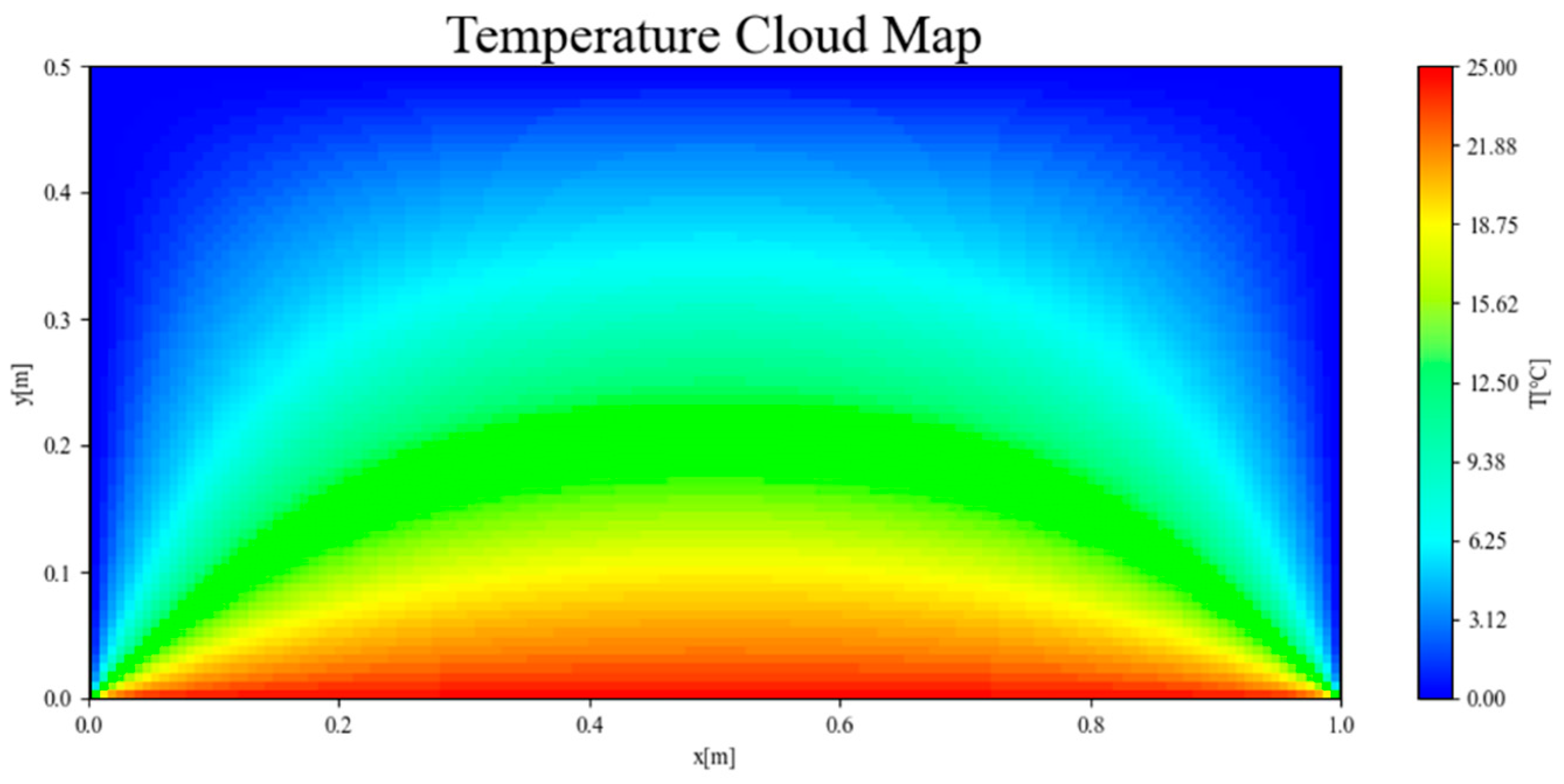
The simulation experiment is configured according to the complete boundary conditions and energy equations in Section 2. The simulation is initiated from the initial conditions and terminated when the temperature reaches a steady state. Subsequently, a temperature distribution contour map, as shown in Figure 2, can be obtained. The results of the contour map indicate that, under the combined action of the four boundary conditions, the overall temperature distribution after heating is symmetrical about the position where x = 0.5. When the observation surface shifts from the symmetrical plane to the left and right sides, the temperature gradient near the heating surface gradually increases, and the left and right walls exert an obvious impact on the overall temperature distribution, which is consistent with the heat conduction law.

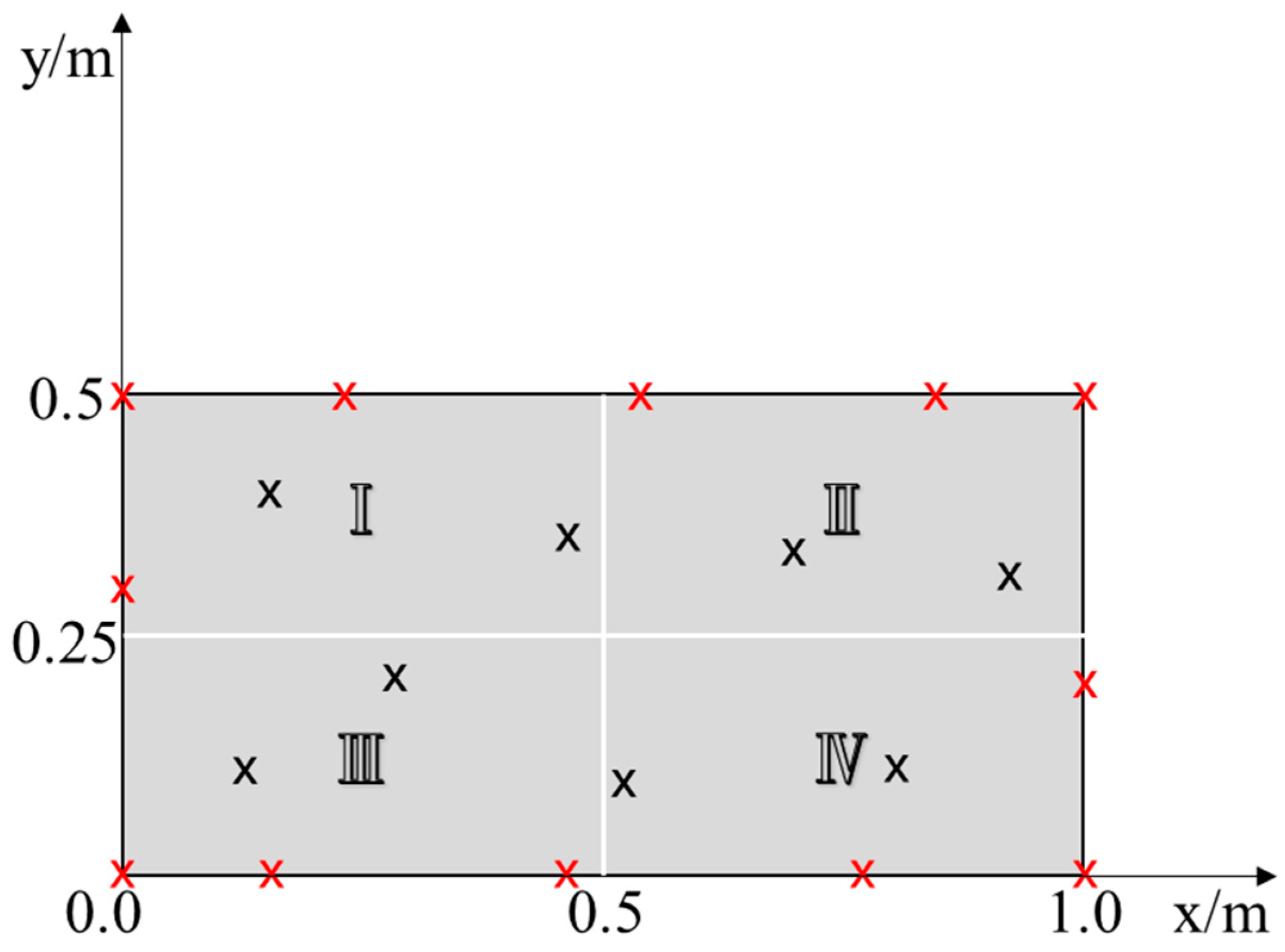
After obtaining the simulation results, we sample the temperature data of 20 coordinate points (approximately 0.2% of finite element nodes) within the plane. In order to improve the accuracy of the model while ensuring universality, restrictions are placed on the positions of the sample points. We draw a vertical line at x = 0.5, and then a horizontal line is drawn at y = 0.25, so that the two lines intersect at the center point of the solution domain, and the solution domain is evenly divided into four symmetrical and mutually independent regions. The four sub-regions are named as I, II, III and IV in the order from left to right and from top to bottom. Fixed points are taken at the four vertices; eight positions are evenly sampled on the four boundaries, and four positions are randomly sampled within the plane. The sample points are represented by ‘x’ in the figure, among which the sample points at the vertices and boundaries are colored red and those within the plane are colored black. The final sampling results are shown in Figure 3. Currently, there are three sample points on the boundary of each sub-region and two inside.

Store the coordinate information and temperature data of the sample points into the temperature database established based on MySQL to complete the acquisition of labeled data to facilitate the subsequent invocation during the inversion calculation.

4.2. Inversion of Boundary Conditions and Temperature Field Based on PINNs Method

For this problem, the network structure illustrated in Figure 4 is set up. The spatial coordinates x and y are taken as inputs, and the object temperature T is the output. The network consists of eight hidden layers, with sixteen neurons in each layer. The tanh function is used as the activation function for all of them. The Adam optimizer is used for optimization. The initial learning rate is set to 0.01, and a polynomial decay strategy [20] with a multiplication factor of 0.8 is adopted to dynamically adjust the learning rate in units of every 10,000 iterations. The loss function is the sum of the differential equation loss, the data loss and the boundary condition loss.

In the PINNs framework, automatic differentiation is a key component that allows the neural network to compute derivatives of the output (temperature T) with respect to the inputs (spatial coordinates x, y). After the neural network outputs the temperature field T(x,y), the automatic differentiation engine uses the computational graph and chain rule to first calculate the first-order derivatives ∂T/∂x and ∂T/∂y and then further compute the second-order derivatives ∂²T/∂x² and ∂²T/∂y². These second-order derivatives are directly used to calculate the residual of the Laplace equation (∂²T/∂x² + ∂²T/∂y²), thereby constructing the PDE loss term. Unlike traditional numerical methods, PINNs do not require finite differences or other numerical approximations to calculate these derivatives but, instead, obtain exact derivative values directly through the neural network’s computational graph, enabling physical laws to be directly embedded into the learning process.

The partial differential equation to be solved in this problem involves first-order and second-order partial derivatives and does not consider the time term. Set the weight ω_nn of each loss term to 1 and use the default weights and biases of the optimizer. The loss function can be expressed as

$$L_{Total}=L_{Data}+L_{PDE}+L_{bc}$$

(12)

$$L_{Data}={\displaystyle \frac{1}{N_{Data}}}{\sum }_{i=1}^{N_{Data}}{\left|u\left(x^i,y^i\right)-u_{Data}^i\right|}^2$$

(13)

$$L_{PDE}={\displaystyle \frac{1}{N_{PDE}}}{\sum }_{i=1}^{N_{PDE}}{\left|{\displaystyle \frac{{\partial }^{2}T}{\partial x^2}}+{\displaystyle \frac{{\partial }^{2}T}{\partial y^2}}\right|}^2$$

(14)

$$L_{bc}={\displaystyle \frac{1}{N_{bc}}}{\sum }_{i=1}^{N_{bc}}\left({\left|u\left(0,y\right)\right|}^2+{\left|u\left(1,y\right)\right|}^2+{\left|u\left(x,0.5\right)\right|}^2\right)$$

(15)

Since the gradients between different boundary conditions in this problem are relatively large, in order to increase the stability of the network, the number of iterations is set to 100,000 rounds, and “hard constraints” are added at the boundaries. It is stipulated that the inversion results of the network do not exceed the upper and lower limits of the set boundary conditions to ensure that the calculations of the PINNs method at the boundaries do not deviate from the constraints of physical laws [21]. The absolute error of each point in the computational domain and the average relative error over the entire domain are selected as indicators to evaluate the performance of the neural network in the temperature field inversion prediction [22]. Since the PINNs method belongs to a stochastic optimization method, its results will be affected by network initialization and random parameter settings, and it cannot be guaranteed that each training result is the global minimum [23]. For the non-convex optimization problem such as parameter training, ten rounds of training are carried out in this problem, and the best result is selected as the training result. During the training phase, the average time required for each solution is two hours, which translates to an average iteration time of 0.072 s per iteration. In comparison to conventional methods that require integration with finite element solvers, this remarkable improvement significantly enhances the computational efficiency of the IHTP. The final temperature field calculation results are shown in Figure 5. The coordinate positions of the labeled data points used by the PINNs method in the training stage are reflected in the temperature contour map as black “x”.

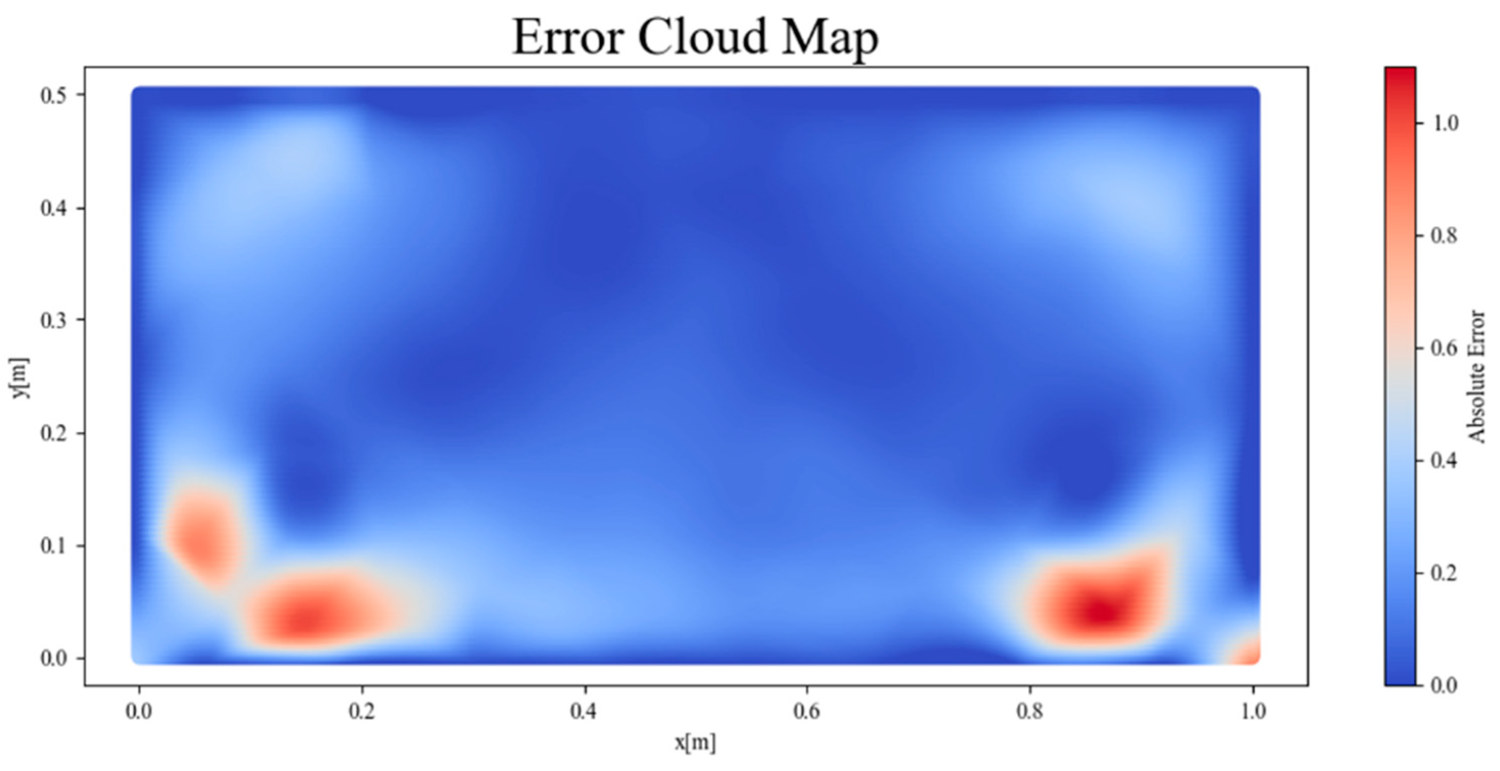
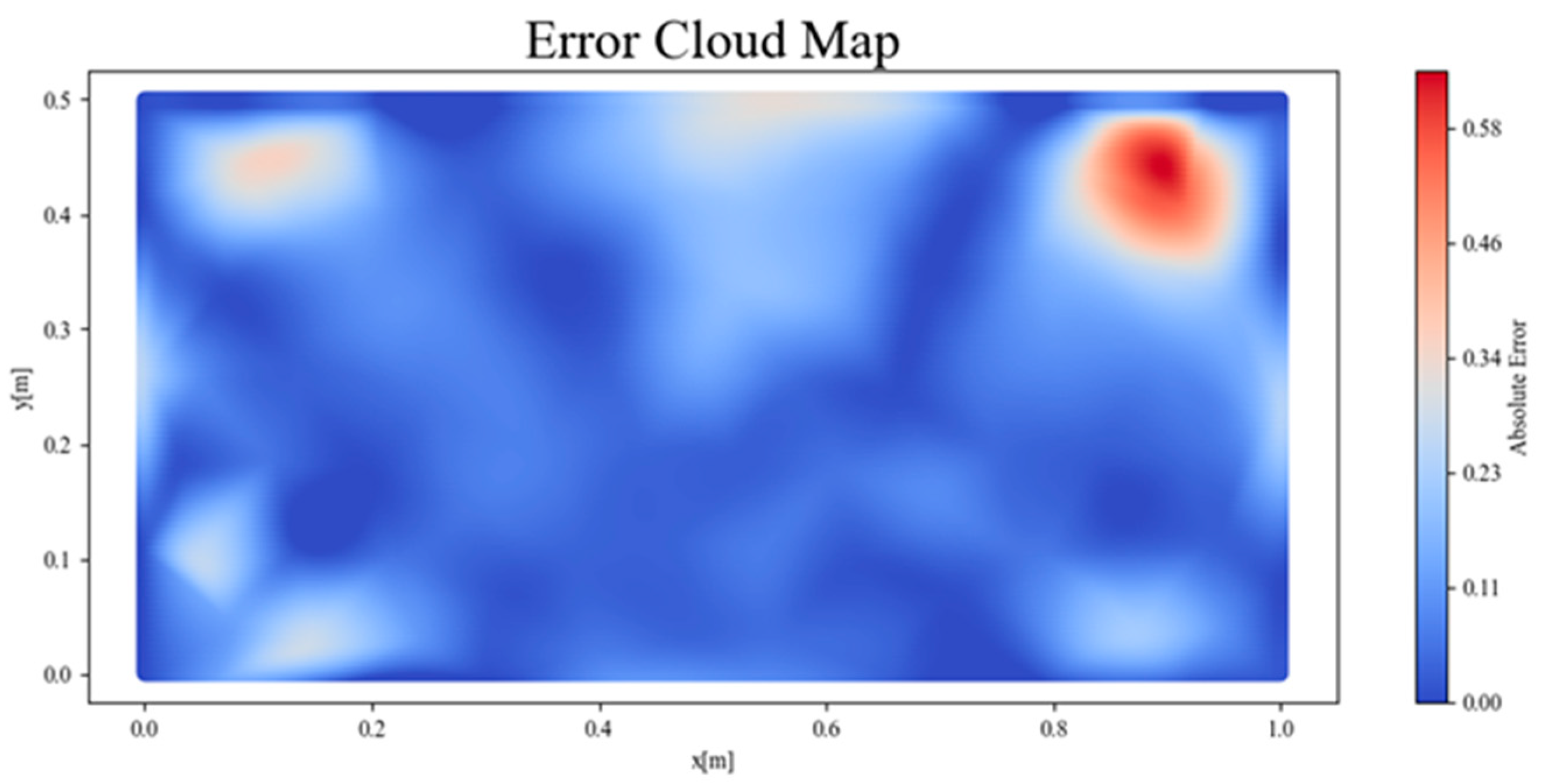
The output of the final loss function $L_{Total}$ in the training process is approximately 5.78. On the premise of ensuring continuity and calculation accuracy, the cubic interpolation method is used to calculate the absolute error distribution at various locations within the plane, as shown in Figure 6. Meanwhile, the average relative error of the plane is calculated to be approximately 7.8%.

The results of the contour map show that the temperature field solved by the PINNs method is basically the same as that solved by the finite element method on the whole. The absolute error at various locations within the plane is typically less than 0.5 °C, and the maximum is around 1 °C, with a relatively uniform distribution. It is proved that the PINNs method can qualitatively predict the temperature distribution of the entire plane well; that is, under the condition of sparse labeled data, it can solve the physical process represented by the PDE through the constraints of the governing equation and boundary conditions, and it achieved the expected effect. However, at the boundary positions, especially at the locations where the temperature gradient changes greatly, such as near the vertices $\left(\mathrm{0,0}\right)$ and $\left(\mathrm{0,1}\right)$ where the bottom boundary and the left and right boundaries meet, there is a relatively large difference in the temperature distribution obtained by the PINNs method and the Fluent solver. This indicates that, when solving problems with missing boundary conditions, large gradients and the superposition of multiple boundary conditions, there remains room for improvement in the inversion accuracy of this network structure.

4.3. Generalized Verification of PINNs Applied for Inverse Heat Transfer Problems

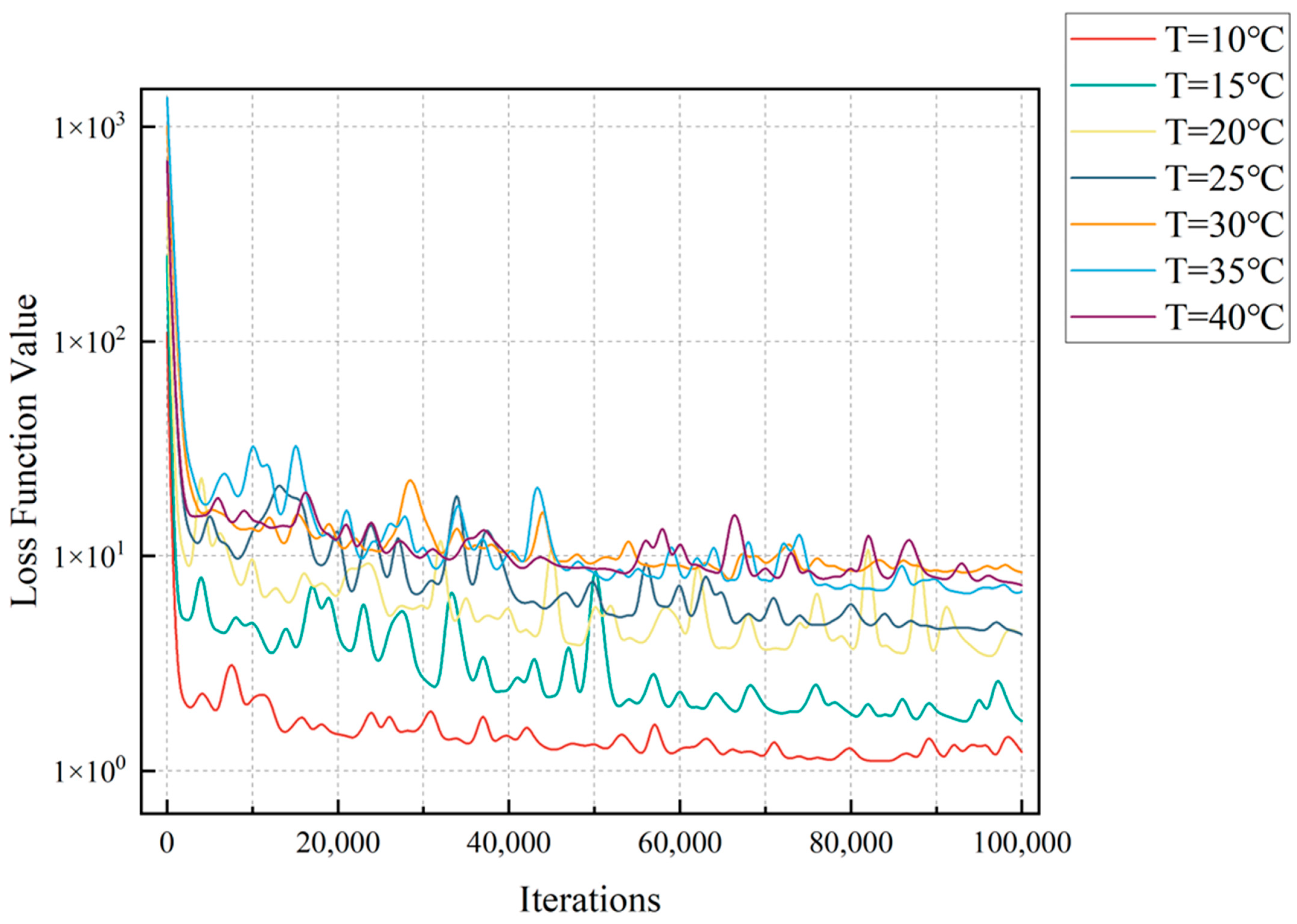
In this research, the temperature boundaries of the heat conduction problem are set to range from 10 °C to 40 °C. In order to study the accuracy of the PINNs method within this temperature range, seven working conditions are established. Starting from 10 °C, with an increment of 5 °C as a gradient, a total of seven working conditions are set. The model generalized verification of the PINNs method is carried out by adjusting the temperature values of the boundary layer. Similarly, in order to ensure the repeatability and stability of the results, ten rounds of training are independently carried out for each working condition, and the loss functions with the minimum average relative errors for each working condition are, respectively, selected and shown in

Table 1. Average relative error and loss function values at different heating temperatures.

Component	Temperature of Heating (°C)	Average Relative Error	$\mathit{L}\mathit{T}\mathit{o}\mathit{t}\mathit{a}\mathit{l}$
1	10	0.070385	1.21974
2	15	0.070473	1.70852
3	20	0.072126	4.31557
4	25	0.077490	4.32680
5	30	0.081967	8.37566
6	35	0.080866	6.81910
7	40	0.081620	7.29384

.

According to the iteration trend of the loss function shown in Figure 7, within this temperature range, the solutions obtained by the PINNs method can all achieve convergence. However, due to the different correlations between features and regression values under different working conditions, the magnitudes of their final convergence values also vary. The larger the temperature gradient is, the larger the final loss function value will be.

In order to observe the impact of temperature gradient changes on the solutions obtained by the PINNs method more intuitively, the temperature distribution contour maps and absolute error contour maps under different working conditions are drawn, respectively, as shown in Figure 8.

Based on the above results, it can be observed that the temperature range set by the boundary conditions will affect the solutions obtained by the PINNs method to some extent. When the temperature gradient increases, the inversion error will rise slightly, but it always remains within 10%. This proves that the PINNs method has a certain generalized ability in this application scenario.

4.4. Impact of Sample Point Positions on the Inversion Results

In the above research, by analyzing the temperature contour map and the absolute error contour map when the bottom boundary condition is 25 °C, it can be observed that the positions with relatively large errors are concentrated at the junctions of the bottom and the side edges. To further reduce the errors and improve the inversion accuracy, the controlled variable method is adopted to explore the impact of the sample point positions on the inversion results.

According to the method of controlling variables, each subdomain is solved individually, and the division strategy is shown in Figure 3. While keeping the number and positions of the sample points on the boundary unchanged, the number of sample points is separately increased in one of the sub-regions each time, so that the number of sample points inside the sub-region triples from the original number. The positions of the sample points in the four solutions and the corresponding absolute error loss contour maps are shown in Figure 9.

The calculation results show that when the sample points are encrypted in sub-regions I and II, the changes in their absolute error contour maps are not obvious. However, after the sample points in sub-regions III and IV are encrypted, the absolute errors in the corresponding regions decrease to a certain extent. This is mainly because the temperature gradient changes greatly at the junctions of the bottom and the side edges, and it is relatively sensitive to the regional temperature changes. If the PINNs method does not obtain enough feature points in this region, it may lead to insufficient inversion accuracy in this region and, thus, cause relatively large errors. Existing research [24] has demonstrated that the PINNs method can solve the forward problem of the heat conduction equation without relying on labeled data when the partial differential equation, initial conditions and boundary conditions are complete. Considering that the goal of the PINNs method is to obtain relatively accurate results using as sparse labeled data as possible, the method of improving the inversion accuracy by adjusting the positions of sample points without increasing the number of sample points is more universally applicable in practical applications.

To further refine the sampling strategy, the solution results of different sub-regions in Figure 9 are summarized. Based on the conclusion that the regions with large temperature gradient changes are more sensitive to temperature changes, a new sampling method is adjusted and obtained. Draw two quarter rounds with a radius of 0.35 m, respectively, with vertices $\left(\mathrm{0,0}\right)$ and $\left(\mathrm{0,1}\right)$ as the centers and the bottom edge and the left and right-side edges as the boundaries. Take these two regions as the regions with relatively large temperature gradient changes within the computational domain. Sample 4 positions evenly in each region to replace the previous eight randomly sampled positions within the plane, and obtain the updated sampling coordinates, as shown in Figure 10. The representation method of the sample points in the figure is also consistent with that in Figure 3.

Using the PINNs method to solve the inverse problem, the obtained absolute error contour map is shown in Figure 11. The error areas and magnitudes within the two quarter rounds have been significantly reduced. At this stage, the average relative error is approximately 6.78%, which is reduced by approximately 1% compared to that before the sample points were updated. This result demonstrates that the positions of the sample points will have an impact on the inversion results. Increasing the sample point density at positions with larger temperature gradients effectively reduces solution errors and enhances inversion accuracy.

4.5. Impact of Adaptively Scaled Weights Based on Learning Rate Annealing Procedure on the Inversion Results

In the research from Section 4.2, Section 4.3 and Section 4.4, the weight ω_nn of each loss term was uniformly set to 1. To some extent, this can simplify the mapping relationship of the PINNs method during the solution process. However, comparing the absolute error between the PINNs method and the labeled data performs poorly in enforcing the boundary conditions, increasing the overall error loss. This is because the ill-posed inverse problem model and the limited labeled data cause conflicts among different parts of the loss function during the training process [25]. The different magnitudes of magnitude of the values of $LPDE$, $Lbc$ and $LData$ lead to unbalanced gradients in the backpropagation of the network. This causes the model’s solution to be severely biased towards the term with the largest gradient, rather than the entire loss function [26]. This will lead to an increase in the errors corresponding to the other two terms, thus affecting the convergence of the PINNs method when applied to solve inverse problems. The principle of the PINNs method is to incorporate physical prior knowledge into the training of the loss function. The most important part, and the core that gives physical meaning to the training process, is the incorporation of the governing equation (PDE). Drawing on the method proposed by Wang et al. [27], we apply the Learning Rate Annealing procedure combined with Adaptive Scaling of Weights to mitigate the interference of unbalanced gradients on convergence.

For the loss function of Equation (12), since $L_{PDE}$ is the core of the convergence of the PINNs method, the gradients of $L_{PDE}$ and $L_{Data}$ are adjusted based on the gradient of $L_{PDE}$. The weight ${\omega }_{PDE}$ of $L_{PDE}$ is set to be constantly 1. At the same time, set the weights ${\omega }_{bc}$ and ${\omega }_{Data}$ (uniformly represented by $\omega nn$ in Equations (17) and (18)) of $L_{bc}$ and $L_{Data}$ as trainable parameters. The new loss function is expressed as,

$$L_{Total}=L_{PDE}+{\omega }_{bc}{L}_{bc}+{\omega }_{Data}{L}_{Data}$$

(16)

During each training session, calculate the gradient values of $L_{PDE}$, $L_{bc}$, and $L_{Data}$, respectively, in backpropagation. Then, based on the correspondence between the maximum value of the gradient of $L_{PDE}$ and the average values of the gradients of $L_{bc}$ and $L_{Data}$, calculate ${\widehat{\omega }}_{bc}$ and ${\widehat{\omega }}_{Data}$ (uniformly represented by ${\widehat{\omega }}_{nn}$ in Equations (17) and (18)), i.e.,

$${\widehat{\omega }}_{nn}={\displaystyle \frac{\mathit{max}\left\{\left|\nabla L_{PDE}\right|\right\}}{\overline{\left|\nabla {\omega }_{nn}{L}_{nn}\right|}}}$$

(17)

where | | is the elementwise absolute value; $\mathit{max}\left\{\left|\nabla LPDE\right|\right\}$ is the maximum value of $\left|\nabla L_{PDE}\right|$; and $\overline{\left|\nabla {\omega }_{nn}{L}_{nn}\right|}$ is the average value of $\left|\nabla {\omega }_{nn}{L}_{nn}\right|$.

Subsequently, the weights are updated using the method of moving average update,

$${\omega }_{nn}=(1-\alpha ){\omega }_{nn}+\alpha {\widehat{\omega }}_{nn}$$

(18)

where α is the weight of the moving average, which is used to control the smoothness of the update. It has a very low sensitivity, and when it takes values within a reasonable range, it will not significantly affect the training results. Generally, α = 0.1.

Other settings remain consistent with those in Section 4.3. The absolute error contour plot obtained by training with the updated loss function is shown in Figure 12. The error at the boundary is significantly reduced. The average relative error is approximately 5.32%, which is about 2% lower than that of the traditional PINNs method. Meanwhile, the maximum absolute error has decreased from approximately 1.0 to approximately 0.6, with a decline rate reaching 40%. This result effectively demonstrates that adjusting the loss function using adaptively scaled weights can mitigate the interference of unbalanced gradients on convergence and enhances the inversion accuracy.

4.6. Generalization to Unseen or Inconsistent Boundary Conditions

Although our validation uses fully specified Dirichlet conditions, the adaptively weighted PINN is naturally suited to cope with perturbed or partially unknown boundaries. First, its sparse data robustness—requiring only ~0.2% of domain samples—ensures stable reconstruction, even when large swathes of boundary measurements are missing or corrupted. Second, our gradient-sensitive sampling concentrates collocation and measurement points in regions of high-temperature gradient (e.g., boundary junctions), helping the network “see” and adapt to unexpected boundary shifts. Finally, the Adaptive Weight Scaling via Learning Rate Annealing dynamically rebalances the PDE, boundary-condition, and data-mismatch losses at each iteration, mitigating conflicts when observed data imply BCs that deviate from training assumptions.

Nevertheless, several challenges remain before tackling truly “unknown” boundaries in practical settings. If actual BCs strongly violate the embedded PDE constraints (for example, abrupt flux changes), the network may have difficulty reconciling physics and data—future work will explore automatic inconsistency detection and on-the-fly loss reweighting. Our current implementation also lacks uncertainty quantification, so integrating Bayesian PINNs or ensemble methods will be crucial to provide confidence bounds on both the reconstructed field and inferred BCs. Lastly, real-world BCs often vary over time; extending our steady-state framework to a time-dependent PINN will be necessary to address transient or periodically perturbed boundary conditions.

5. Conclusions

This research investigates the application of Physics-Informed Neural Networks (PINNs) for solving inverse problems in two-dimensional steady-state heat conduction. Our key findings include the following:

(1)

PINNs effectively solve inverse heat transfer problems within a temperature range of 10 °C to 40 °C with high computational efficiency (0.072 s per iteration). The method maintains absolute errors below 1 °C and average relative errors under 10% across the computational domain, providing a viable alternative to traditional CFD methods for rapid PDE solutions in engineering applications.

(2)

The strategic optimization of sampling point distribution enhances solution accuracy without increasing data requirements. By concentrating sampling points in regions with steep temperature gradients, we achieved an approximately 1% reduction in the average relative error, offering practical implications for experimental design and sensor placement.

(3)

Our adaptive weight scaling strategy based on learning rate annealing addresses unbalanced gradients in the loss function, reducing the maximum absolute error by 40% (from 1.0 °C to 0.6 °C) and decreasing the average relative error by approximately 2%.

The PINNs method demonstrated in this study offers several key advantages for inverse heat transfer problems: computational efficiency (0.072 s per iteration), ability to work with sparse measurement data (just 0.2% of domain nodes), integration of physical laws ensuring physically consistent solutions, and flexibility in handling unknown boundary conditions. However, the method also presents certain limitations: sensitivity to sample point distribution requiring strategic placement in high-gradient regions, challenges in balancing different components of the loss function, stochastic optimization nature necessitating multiple training runs, and dependence on careful hyperparameter tuning for optimal performance.