1. Introduction
Paragliding sails are characterized by a deformable fabric wing. It is held in position by rigid vertical textile ribs that provide form and structural properties to the fabric. The inflation of the wing is guaranteed by an opening in the bottom side of the wing, which allows mass exchange between the inside part of the wing and the outside part. Standard flight conditions involve slightly positive angles of attack in order to enable canopy inflation and lift generation. In addition, canopy filling is allowed by the location of the stagnation point in the air inlet region, which leads to a pressure value similar to the undisturbed flow’s total pressure. Undesirable operating conditions can produce paraglider deflation. Specifically, a passage through a thermal column or the presence of atmospheric turbulence can produce a depression zone induced by a negative angle of attack or an aerodynamic stall. The canopy’s leading edge closes, and the wing deflates over itself. It is very easy to understand that the prediction of issues related to canopy closure is a key problem in this context.
The seminal papers in the literature are mainly devoted to ram-air gliding parachutes [
1,
2,
3,
4,
5,
6,
7,
8,
9,
10]. In these studies, wind tunnel tests were carried out for full fabric or semi-rigid models; in particular, the influence of aspect ratio, angle of attack, and air inlet on aerodynamic wing performance were studied. Based on these experimental results, Lingard [
11] developed a theoretical investigation on ram-air parachute aerodynamics for delivery systems. Some other papers on paraglider airfoils have been published [
12,
13,
14,
15,
16,
17]. Belloc [
12] performed an experimental study focused on the evaluation of the spanwise arched shape in terms of longitudinal and lateral stability. It is worth noting that the author used a non-deformable wind tunnel model. Mashud and Umemura [
13] carried out internal and external pressure measurements on an inflatable model, also considering the variation in the shape of the fabric. Belloc et al. [
14] performed a large numerical investigation to evaluate the influence of the position and dimension of the air intake on aerodynamic performance. Boffadossi et al. [
15] optimized the air inlet of a paraglider using numerical and experimental approaches. Abdelqodus et al. [
16] presented a numerical study on the performance improvement produced by the shark-nose technology compared to a typical inlet. Hanke and Schenk [
17] used a photogrammetry to study the in-flight shape of a full-scale paraglider wing.
In this study, we present an experimental wind tunnel investigation that we conducted with the goal of qualitatively evaluating the fabric deformation of an inflatable wing for paragliding. We also wanted to study how these deformations are correlated with aerodynamic performance and boundary layer separation phenomena. In particular, our interests concern the inflation/deflation phases and local deformations. The inflation and deflation phases concern the whole wing, and they were detected through a piezoelectric sensor placed on the wing surface. In contrast, local deformations necessitated the use of non-contact measurements in order not to influence the fabric’s behavior. We applied infrared thermography to detect local surface deformations and boundary layer separation phenomena. Experimental tests were carried out on a Clark Y airfoil, which is not commonly adopted in the paragliding community; in the present study, it was selected because there is a large experimental dataset regarding this airfoil in the open literature. This element made it possible to compare the open wing aerodynamic performance with its standard rigid version.
The paper is organized as follows.
Section 2 describes the experimental setup.
Section 3 shows the results obtained. Finally,
Section 4 contains the conclusions.
2. Materials and Methods
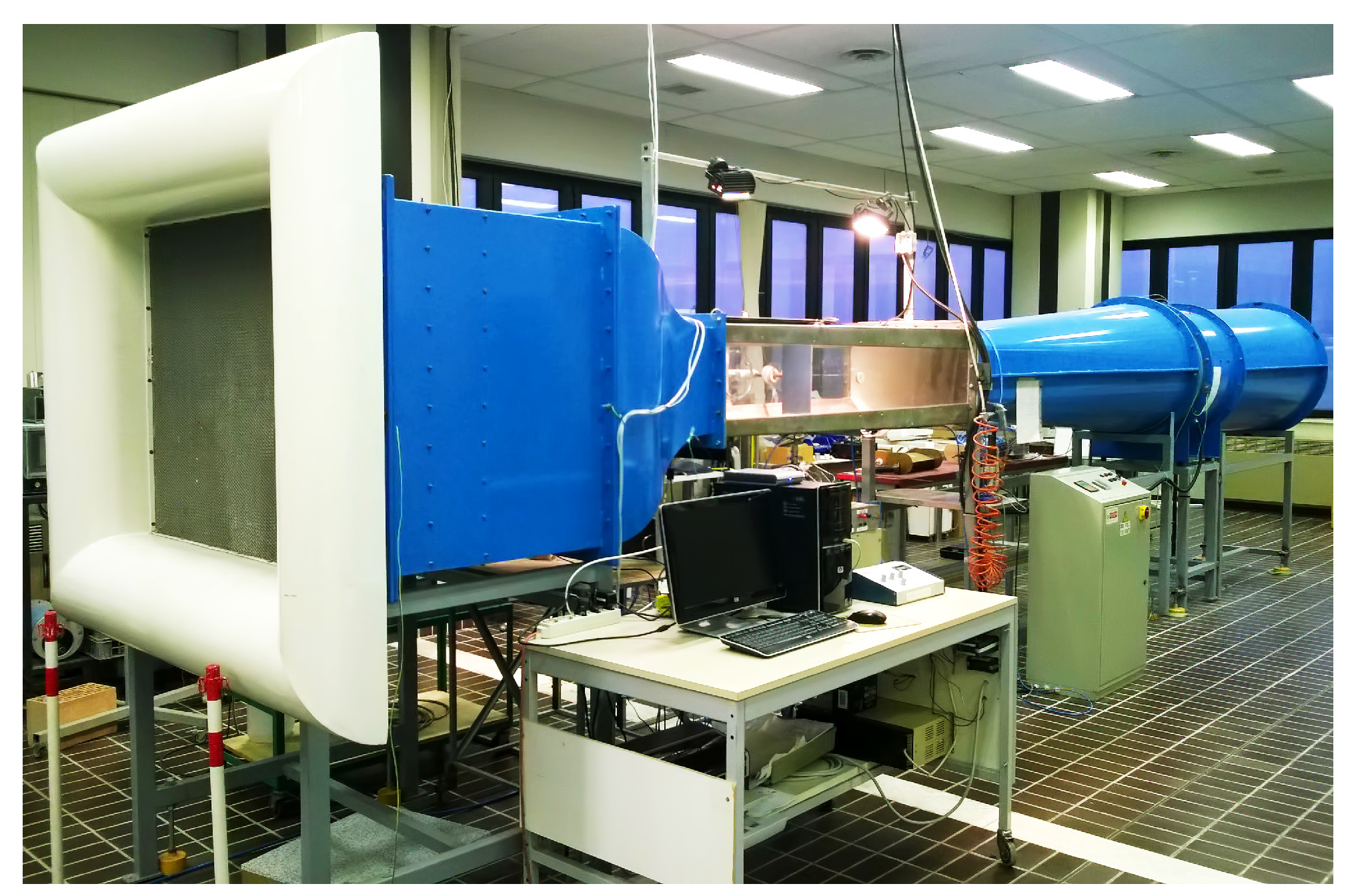
Aerodynamic tests were carried out to correlate fabric deformations with the performance of the wing section. In particular, a load balance was used for the measurement of the lift, drag, and moment coefficients. A wake rake device was adopted to evaluate the velocity in the wake region and the drag coefficient. All tests were carried out in the wind tunnel available at the Dipartimento di Ingegneria Industriale e Scienze Matematiche of Università Politecnica delle Marche (
Figure 1). This facility is an open-circuit subsonic wind tunnel with a test section of 620 mm in width, 380 mm in height, and 1500 mm in length. The maximum velocity at the inlet is 38 m/s, and the mean turbulence in the inlet section is 0.3%.
The uncertainties and full scales of the load balance are listed in
Table 1. Pressure measurements for flow velocity and wake rake analysis were carried out with a Druck LPM 9481 (Baker Hughes, Houston, TX, USA) differential pressure transducer. The instrument uncertainty is ±0.1% of the full scale, ranging from 0.1 Pa to 1000 Pa.
Thermographic measurements were performed through the ’Heated Thin-Foil’ technique. This method uses a fixed heat flux boundary condition on the wing surface, achieved through Joule heating inside a thin electrically conductive layer applied to the wing. In this way, it is possible to correlate the temperature distribution over the wing with boundary layer separation phenomena as a unique function of the convective heat transfer coefficient, h [
18,
19,
20]. From the h value and temperature behavior, it is possible to obtain information about the dimensions and position of the laminar separation bubble (LSB). Indeed, inside the LSB, the air is in a quasi-static condition, and the h coefficient is lower. The result is very low heat dissipation by convection and a high-temperature zone.
Thermographic measurements were performed with an SC3000 FLIR camera (Teledyne FLIR, Wilsonville, OR, USA). The camera is equipped with a 320 × 240 QWIP sensor array and a lens with a 20° × 15° field of view. The minimum focus distance is 0.3 m. The thermal sensitivity is 20 mK at 30 °C with an uncertainty equal to ±1% of the measured value. For each angle of attack (
), investigated, 100 thermographic images were acquired at a frequency of 50 Hz. The frames were then post-processed with MATLAB R2021bcode. The post-processing allowed an initial cleaning of the noise by averaging all the images acquired; then, a filter was applied to remove any spike smaller than the camera’s resolution (20 mK) between two subsequent pixels. A finite difference method was used on a selected straight line on the profile chord in order to solve the energy conservation equation and obtain the distribution of the convective heat transfer coefficient [
21]. This procedure has two critical points: the local view factor and the detection of the wing’s leading and trailing edges. The view factor varies with the angle of attack and along the wing chord due to the surface curvature.
Figure 2 shows the view factor calculated for two cases: a Clark Y airfoil at 0° and a flat plate. The ratio between them was also reported for each pixel. The ratio value indicates that the measurement error introduced by the view factor is negligible from the 10% mark of the chord to the trailing edge, where the LSB is usually located. However, no point before the 10% mark of the chord can be considered reliable, since the view factor of the suction side assumes very low values. The second source of uncertainty is the detection of the leading and trailing edges of the wing section. To reduce this uncertainty, hot points were placed near the model’s leading and trailing edges for each angle of attack investigated (
Figure 3).
The infrared camera was placed outside the wind tunnel at a distance of 0.67 m from the profile. The resulting spatial resolution on the wing surface, corresponding to the size of one pixel, was 0.65 mm. A ZnSe infrared optical window measuring 150 mm long, 50 mm wide, and 4 mm thick was applied to the plexiglass wall of the wind tunnel to observe the wing section. The infrared window had a transmissivity coefficient of 0.70 in the camera’s wavelength range, as measured using a black body. Finally, a high-current, low-voltage power supply was used to uniformly heat the wing surface by the Joule effect using a thin conductive fabric layer applied over the model. This fabric was an EMI shielding fabric made of a nylon ripstop base material with a conductive copper–nickel layer. The fabric had a total thickness of 0.135 mm, a surface resistivity of 0.08 /m2, and thermal conductivity equal to 40 W/mK. The fabric’s emissivity, experimentally measured, had a value of 0.85. Voltage and current were constantly monitored in order to have the same electric power for all tests, equal to 168 W/m2.
2.1. Description of Models
The wing section was a Clark Y airfoil whose chord and span dimensions were 200 mm and 376 mm, respectively. The chord dimension was chosen to avoid excessive wind tunnel blockage, whereas the spanwise dimension was set equal to the wind tunnel’s height to reduce the finite wing effect without the use of end plates.
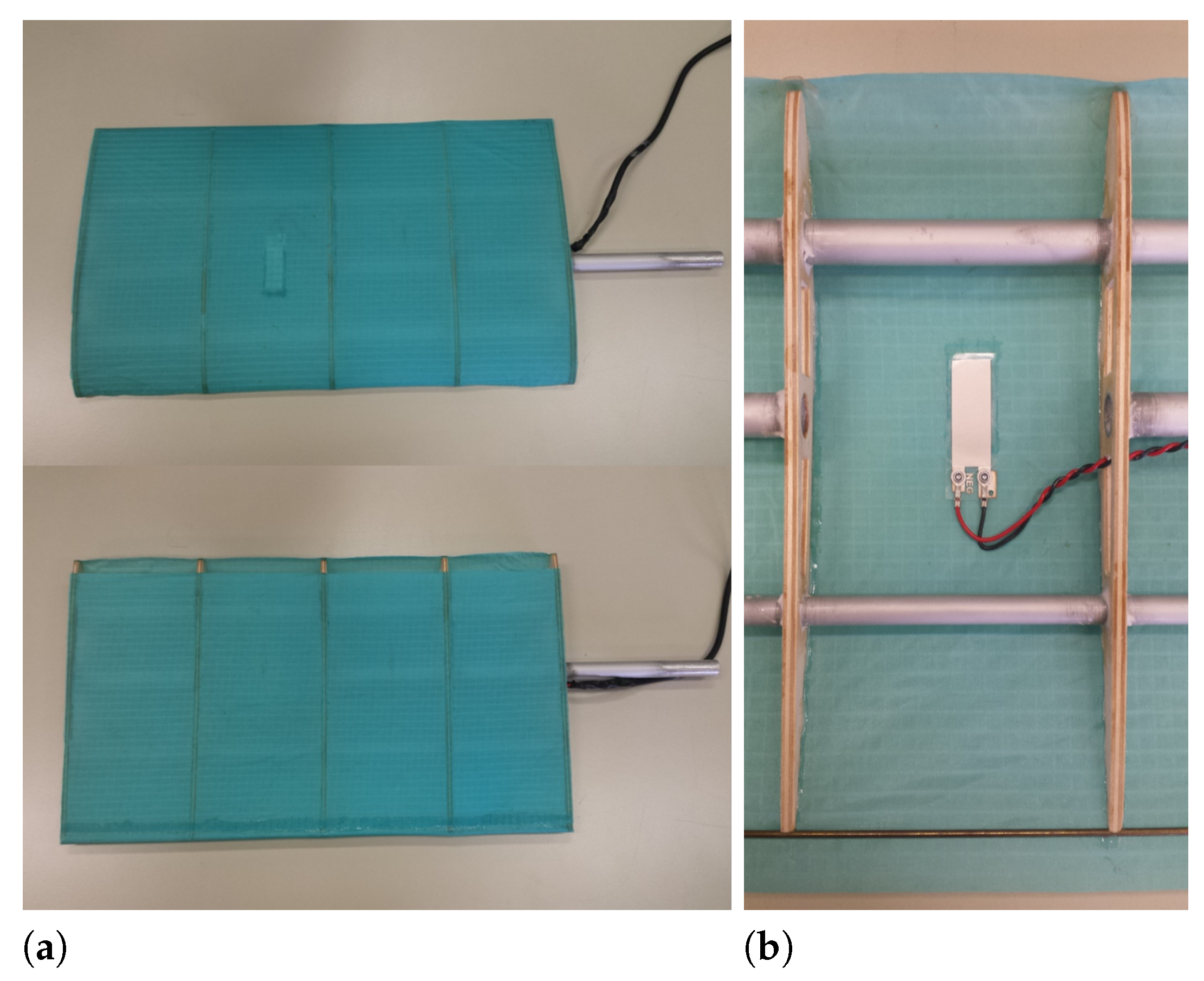
An initial model (model A) was built for aerodynamic tests and inflation/deflation phase detection with a piezoelectric sensor. This model was a semi-rigid wing made of a solid structure covered with a real paragliding fabric. The solid structure consisted of five wooden ribs equally spaced and mounted on three aluminum rods. The air intake was applied from the 1% mark to the 6% mark along the chord length, which is the usual range for paragliding. The piezoelectric sensor was placed on the inner side of the suction side from the 32.8% mark to the 50.5% mark along the chord length (
Figure 4).
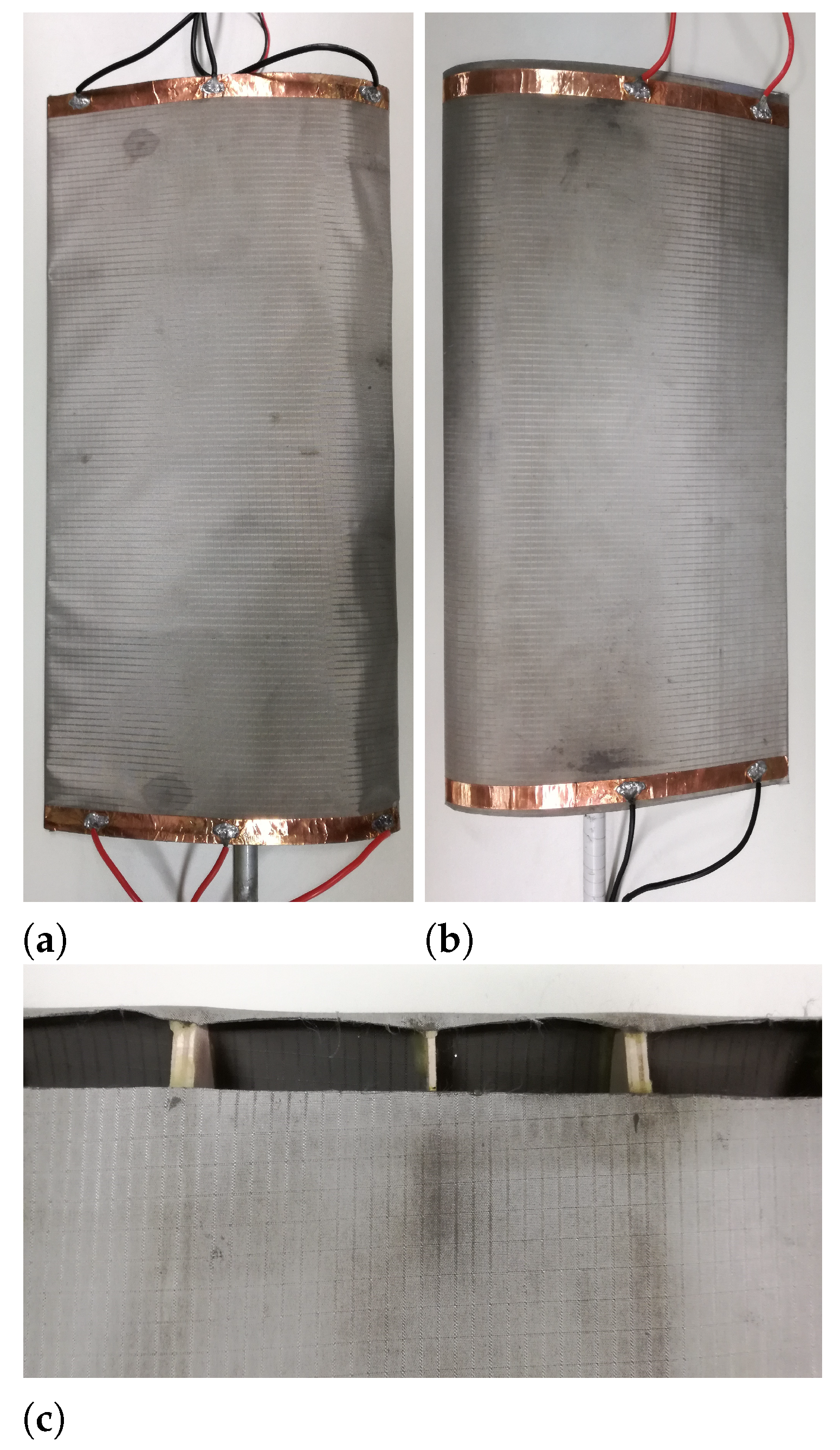
Thermographic analyses were performed on two different models. A rigid one (model B) was built as a reference for the LSB’s position and temperature distribution. It was made of polyurethane foam cut with an automated hot wire machine. Two wooden ribs were placed at the wing border. Finally, a fiberglass lamination process was used to reinforce the structure, and the wing was then covered with the conductive fabric. The inflatable model (model C) is a semi-rigid wing with the same rigid structure as model A. However, the rigid structure was coated with the conductive fabric for this model. The air intake was always applied from 1% to 6% of the chord length. A balsa nose with a width of 1.5 mm was placed between each consecutive pair of ribs to prevent excessive deformation of the leading edge (
Figure 5). To ensure current flow from the power supply to the fabric, copper tape was applied on the spanwise tip of the wing surface. This tape consisted of thin copper foil (25
m) placed over a conductive acrylic pressure- sensitive adhesive. Two welded wires for each copper tape allowed electrical connections.
2.2. Piezoelectric Signal Measurement
The voltage signal produced by the piezoelectric sensor was acquired with a Fluke oscilloscope, model 199C, after passing through a preamplifier. The time base of the instrument was set to the minimum available, corresponding to 5 ms/div. The total acquisition time was 6 s, and the sample rate was equal to 10 kHz. The vertical sensitivity (V/div) was set as a function of the signal amplitude to avoid loss of resolution.
The instrument’s bandwidth can be set to 200 MHz or 10 kHz. For both bandwidths, the signal was acquired first without the piezoelectric sensor (test 1); then, the sensor was connected but not loaded (test 2). The results are shown in
Table 2. It can be seen that for test 2, there was an increase in the mean and standard deviation for the bandwidth of 200 MHz. This did not occur at a bandwidth of 10 kHz, and the standard deviation was an order of magnitude lower than in the first case. For these reasons, the 10 kHz bandwidth was adopted.
Finally, the signal was filtered with a preamplifier in order to eliminate the high-frequency components and clearly detect the inflation/deflation phases of the wing section.
Figure 6 shows the cases with and without filtering while alternately passing from a situation of inflation to a situation of deflation. The signal filtering at 10 Hz made it possible to clearly detect the inflation/deflation phases. Furthermore, from 10° to −4°, the wing deflated, and the peak was positive; in contrast, from −4° to 10°, there was inflation, and the peak was negative.
3. Results
The tests were carried out at two different Reynolds numbers:
and
. The investigated angles of attack varied from −12° to 12°, with an angular step size of 2°. The maximum occupation of the wind tunnel section was 6.5%; accordingly, a blockage correction was applied [
22]. The correction introduced variation of the free-stream dynamic pressure and of the actual angle of attack that differed from the geometric one in load balance tests. Equations (
1) and (
2) were used to apply these corrections:
where
is the geometric angle of attack,
is the measured dynamic pressure, V is the model volume, and W and H are the test chamber’s width and height. The coefficients
,
,
, and
depend on the test chamber’s dimensions [
22]. Furthermore, in Equations (
1) and (2),
and
are the lift and drag coefficient, respectively.
To evaluate the effect of air intake, tests were also performed after closing the air intake with adhesive tape. In the following, the label "open wing" refers to the models with the air intake open; in contrast, the label "closed wing" is adopted for the models with tape covering the air intake.
3.1. Detection of Inflation and Deflation Phases
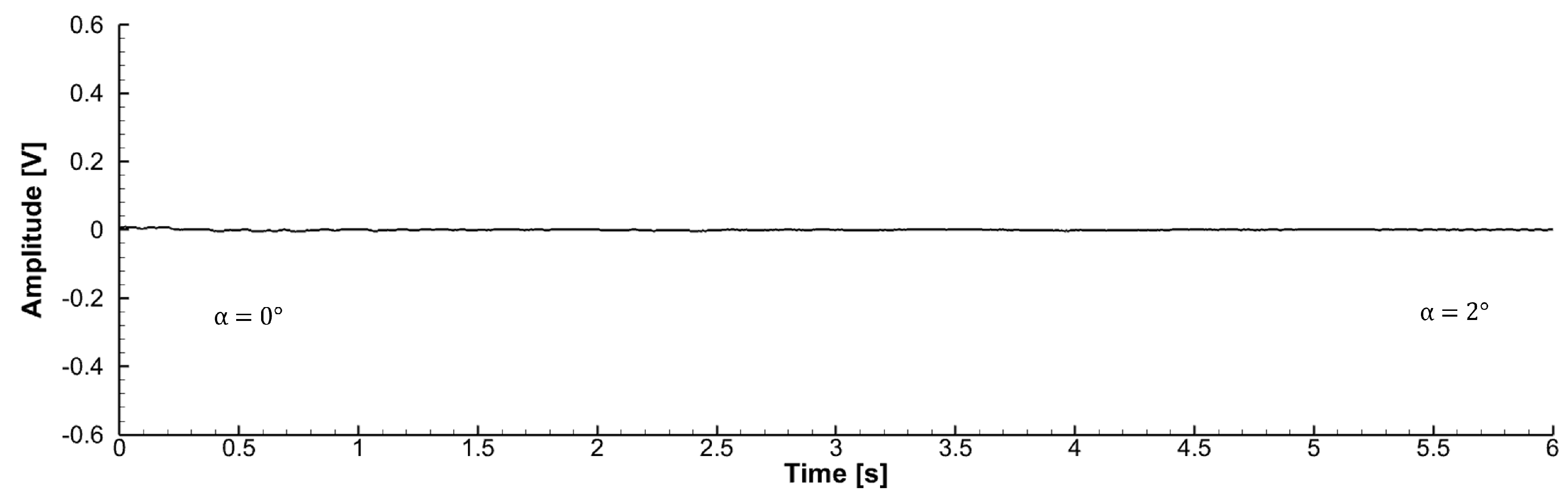
The piezoelectric sensor tests were performed as the angles of attack were increased and decreased with an angular step size of 2°. The inflation/deflation phases are dynamic phenomena, and they occur while the angle of attack is changing. For this reason, the signal of the piezoelectric sensor was acquired for 6 s during the wing rotation, and the signal was presented as a time history. In particular, the acquisition procedure was as follows: the acquisition of the piezoelectric signal began at a certain angle of attack; then, the model was rotated to change the angle of attack; finally, the acquisition was stopped. The process was repeated for each considered variation in angle of attack, by keeping the wind on throughout the test. It is important to note that the angle of attack was changed with a pitching and posing technique during signal acquisition. The first preliminary test was performed by changing the angle of attack in a wind-off condition.
Figure 7 shows the piezoelectric signal obtained for one angle-of-attack variation. It is important to note that there is no peak in the signal for the wind-off condition. This result ensures that a peak in the signal of the piezoelectric sensor is only caused by the inflation/deflation phases and is not related to a deformation of the model’s structure due to the angle-of-attack variation.
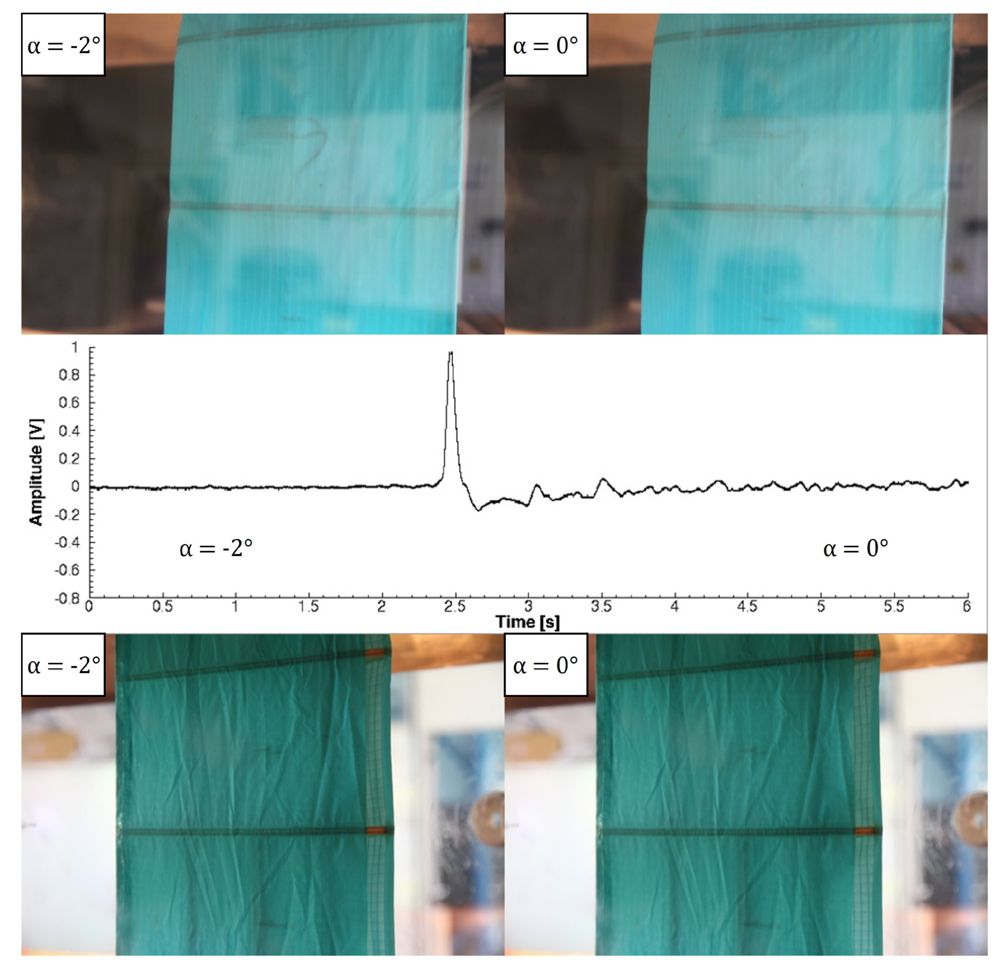
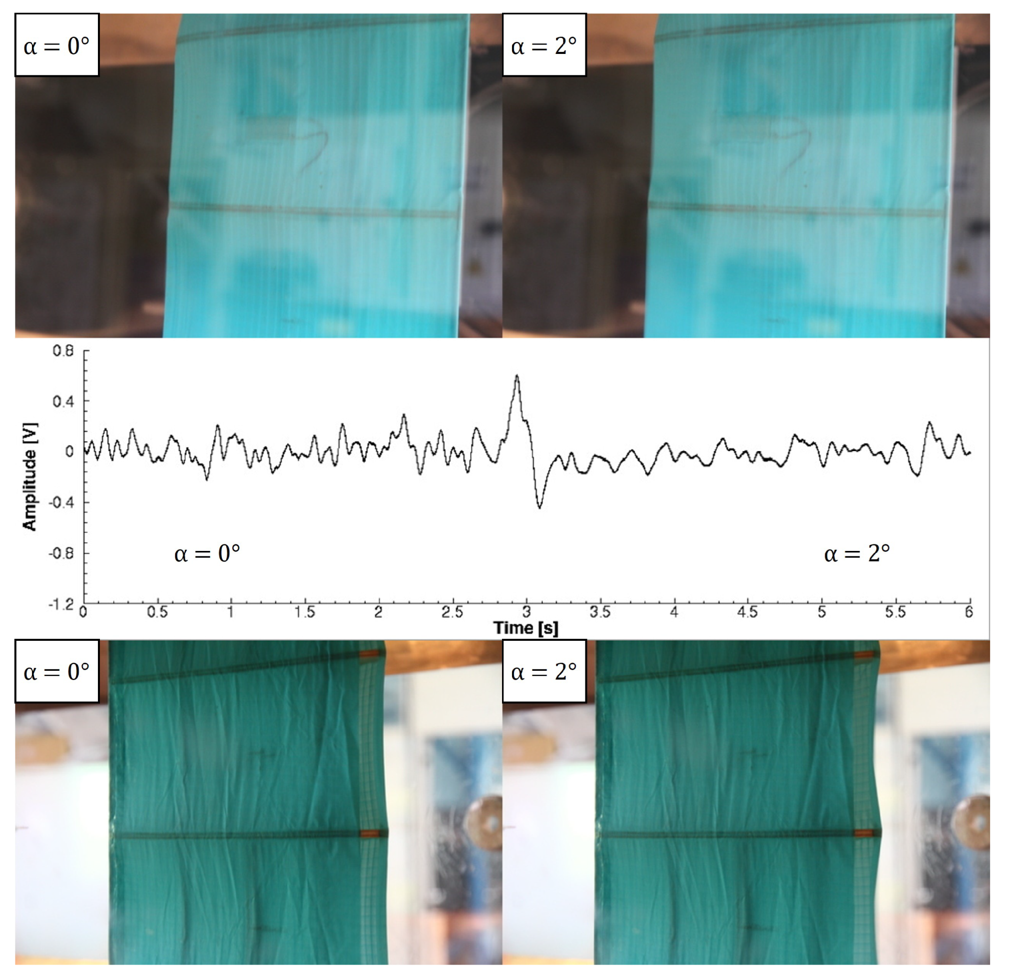
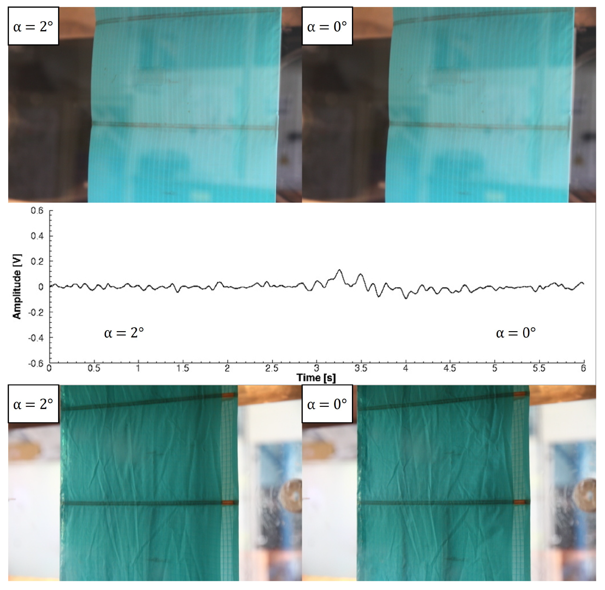
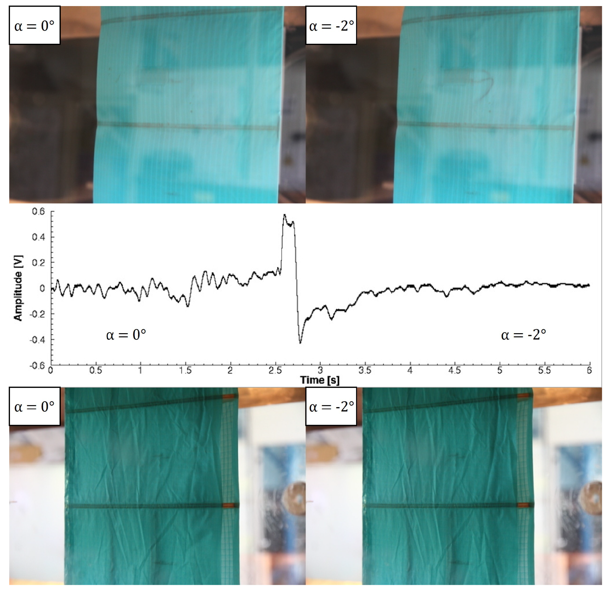
The following figures show the most relevant results and are composed of five elements:
- •
The top zone contains images of the wing’s suction side at initial and final angles of attack (indicated on the images) in the left and right positions, respectively;
- •
The central zone presents the voltage signal generated by the piezoelectric sensor;
- •
The bottom zone is organized in the same manner as the upper one, but the images are relative to the wing’s pressure side.
For Re =
and increasing angles of attack (
Figure 8 and
Figure 9), there is an initial positive voltage peak between −2° and 0°. A positive peak would correspond to a wing deflation, but the image shows the opposite behavior. However, the inflation is limited to the leading edge zone, and the piezoelectric sensor experiences a deformation similar to that in the deflation case. Subsequently, between 0° and 2°, the entire suction side inflates, and the piezoelectric sensor produces a negative voltage peak. For Re =
(
Figure 10 and
Figure 11), between 0° and 2° there is a positive voltage peak corresponding to a partial inflation of the suction side in the leading edge zone. Moving from 2° to 4°, there is a simultaneous inflation of the wing suction and pressure side and the piezoelectric signal shows a negative voltage peak.
For Re =
and decreasing angles of attack (
Figure 12 and
Figure 13), there is a first small positive voltage peak between 2° and 0°, and the pressure side deflates. Then, the suction side of the wing collapses, and there is a higher voltage peak (between 0° and −2°). The different amplitudes of the two peaks can be explained by the fact that the piezoelectric sensor is placed on the suction side. It is more affected by the deformations on this side. The test points out that a deformation on the opposite side can also be detected by the piezoelectric sensor, but with lower magnitude. In Re =
(
Figure 14 and
Figure 15), the trend is similar except for a change in angles. In particular, from 0° and −2°, only the pressure side deflates; moreover, at −2° and −4°, the suction side collapses. The piezoelectric sensor detects both these deformations with a higher voltage peak for the first case than the second, and the same is true for the Re =
configuration.
For all the cases studied, the signal amplitude of the piezoelectric sensor increased with the Re because of the higher velocity and the forces involved. However, for the case reported in
Figure 8, there was different behavior. The signal amplitude of the piezoelectric sensor was higher for the Re =
than the corresponding case at Re =
(
Figure 10). This anomaly could be due to a larger zone of inflation near the leading edge, which involves a larger part of the piezoelectric sensor. The result is a higher deformation and a signal amplitude increase.
3.2. Measurement of Aerodynamic Coefficients
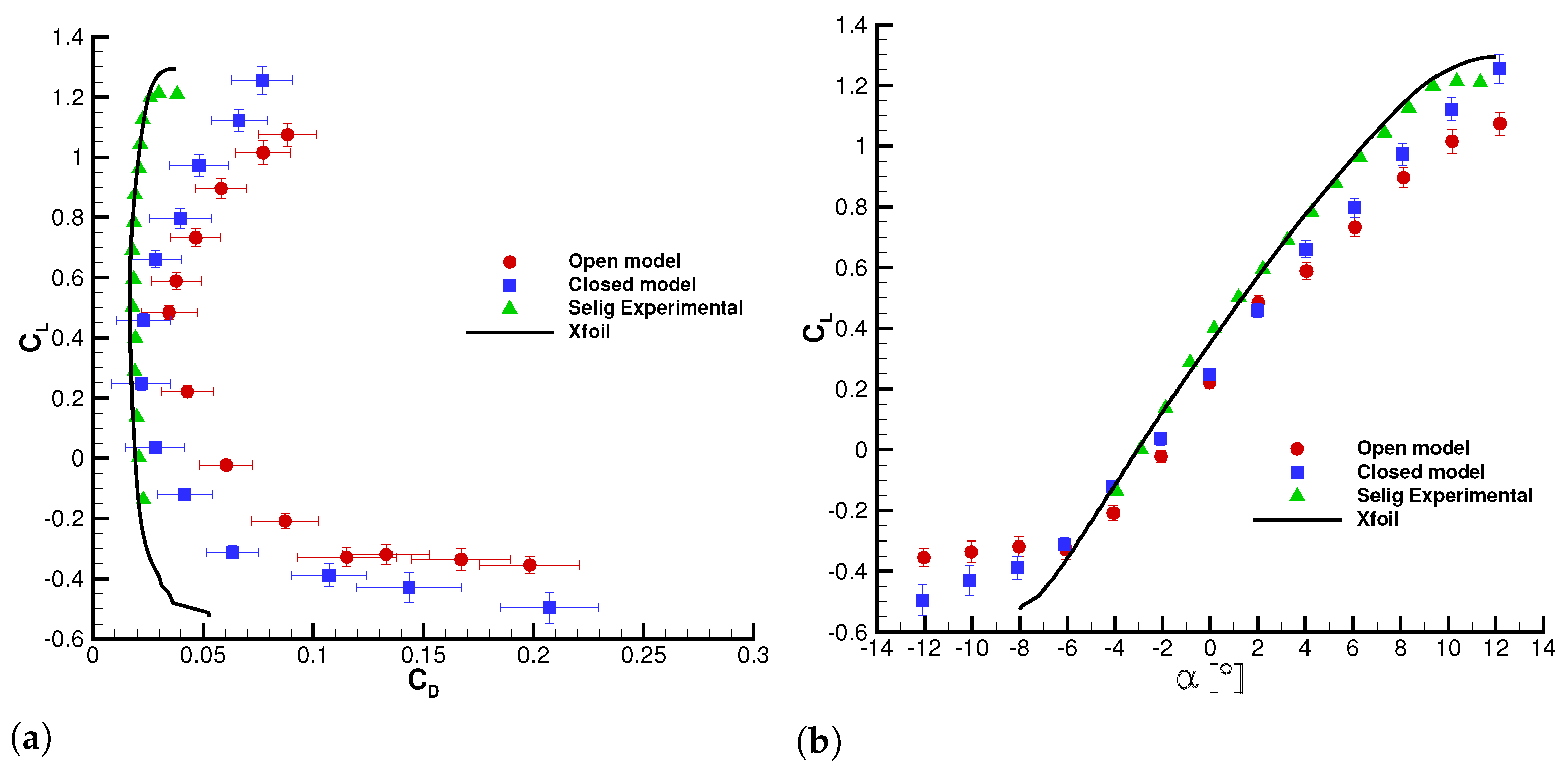
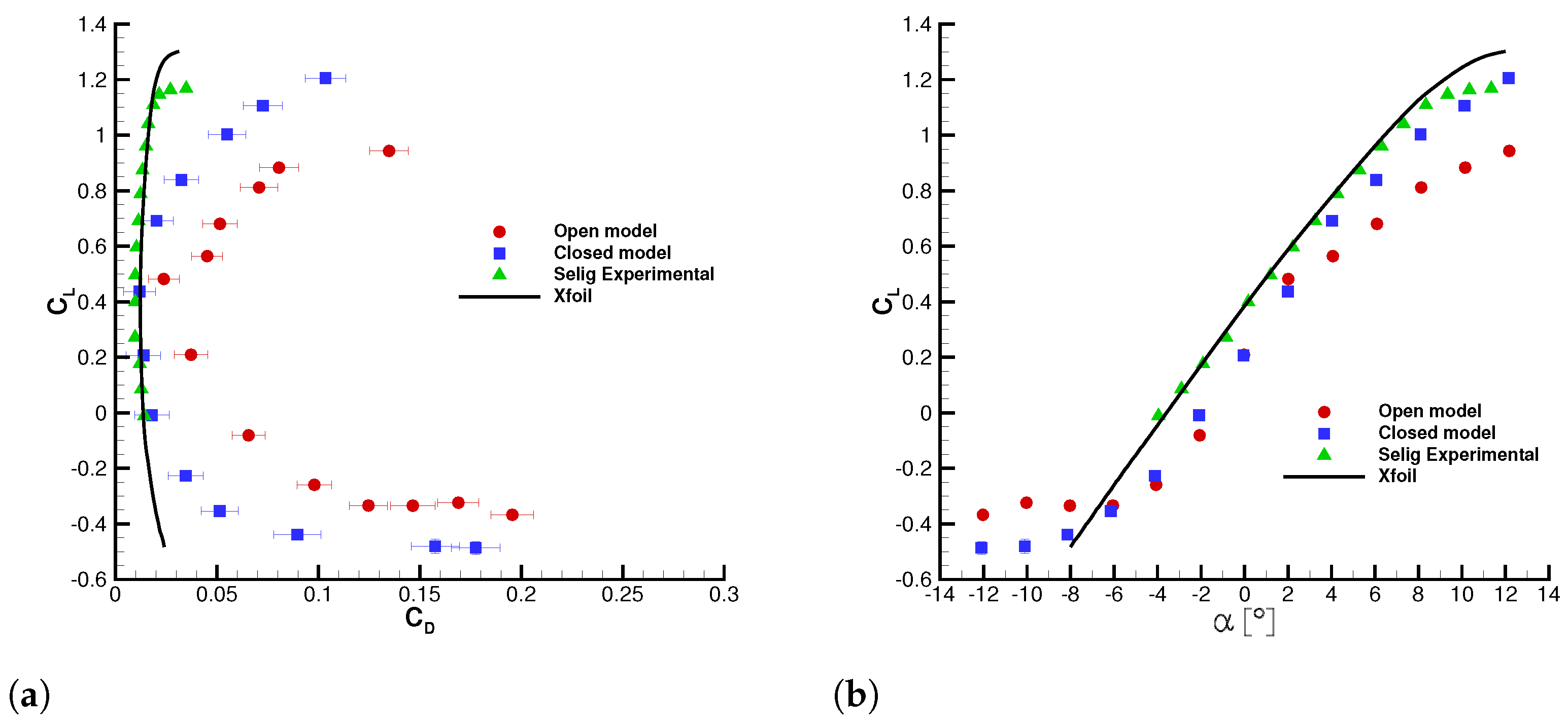
The results are shown in
Figure 16 and
Figure 17, where the experimental data are compared with literature data of a rigid wing [
23] and an Xfoil numerical simulation. It is worth noting that
,
, and
represent the lift, drag, and moment coefficient, respectively.
where
L and
D are the lift and drag force,
is the moment at 25% of chord length,
is the air density,
is the free-stream velocity,
b and
c are the model span and chord dimensions.
The – curves are shifted to the right for both close and open wings and the zero-lift angle is higher than the rigid model. At these angles of attack, the wing is deflated and the surface is pressed against the model structure. Therefore, the wing camber is reduced, and the zero lift angle increases. From 2° to 4° there is also a change of – curve slope only for the open wing. At the same time, there is complete inflation of the wing section, as shown by the piezoelectric data. This explains the change of slope, which is related to the different shape assumed by the wing. A similar behavior was also noted at Re = ; it is important to note that the effect is more evident due to the greater deformation.
The Eiffel polar diagrams show an increase of for all considered angles of attack. This is particularly true for higher angles of attack. Specifically, the aerodynamic drag increases because of the leading edge deformation and the high surface roughness of the fabric. The open wing has always a greater drag coefficient, but the difference with closed wing one is more marked at negative angles of attack. The increase of and the decrease of values reduces the aerodynamic efficiency, as confirmed by a more closed – curve. The aerodynamic efficiency is higher for the rigid wing and decreases for the soft models; in particular, the open wing has the lowest efficiency.
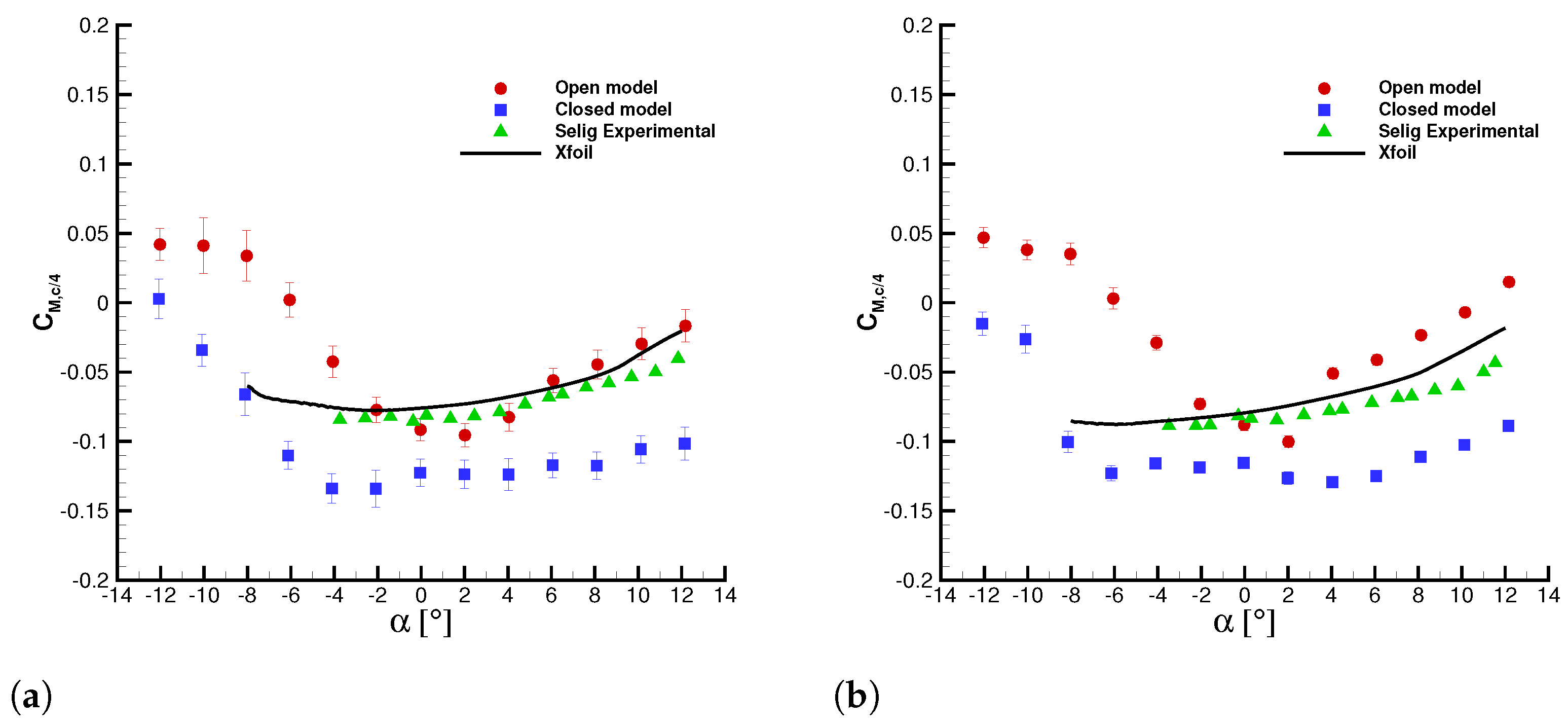
Finally,
Figure 18 shows the
coefficients of open and closed wings. The open wing does not put in evidence a zone of constant values for the angles of attack considered. In contrast, the closed wing exhibits a constant
at positive angles. The rigid wing also shows a constant value of moment coefficient at low angles of attack with a small increase towards positive angles of attack. The magnitude of the
increases when a flow separation appears. A similar behavior was also observed for the closed wing for negative angles of attack, but for the open wing configuration this phenomenon is anticipated. It is important to note that a drop in the moment coefficient is observed when the open wing inflates. This behavior is very evident at Re =
due to the higher aerodynamic forces involved. The moment coefficient drop does not appear for the rigid and closed wings.
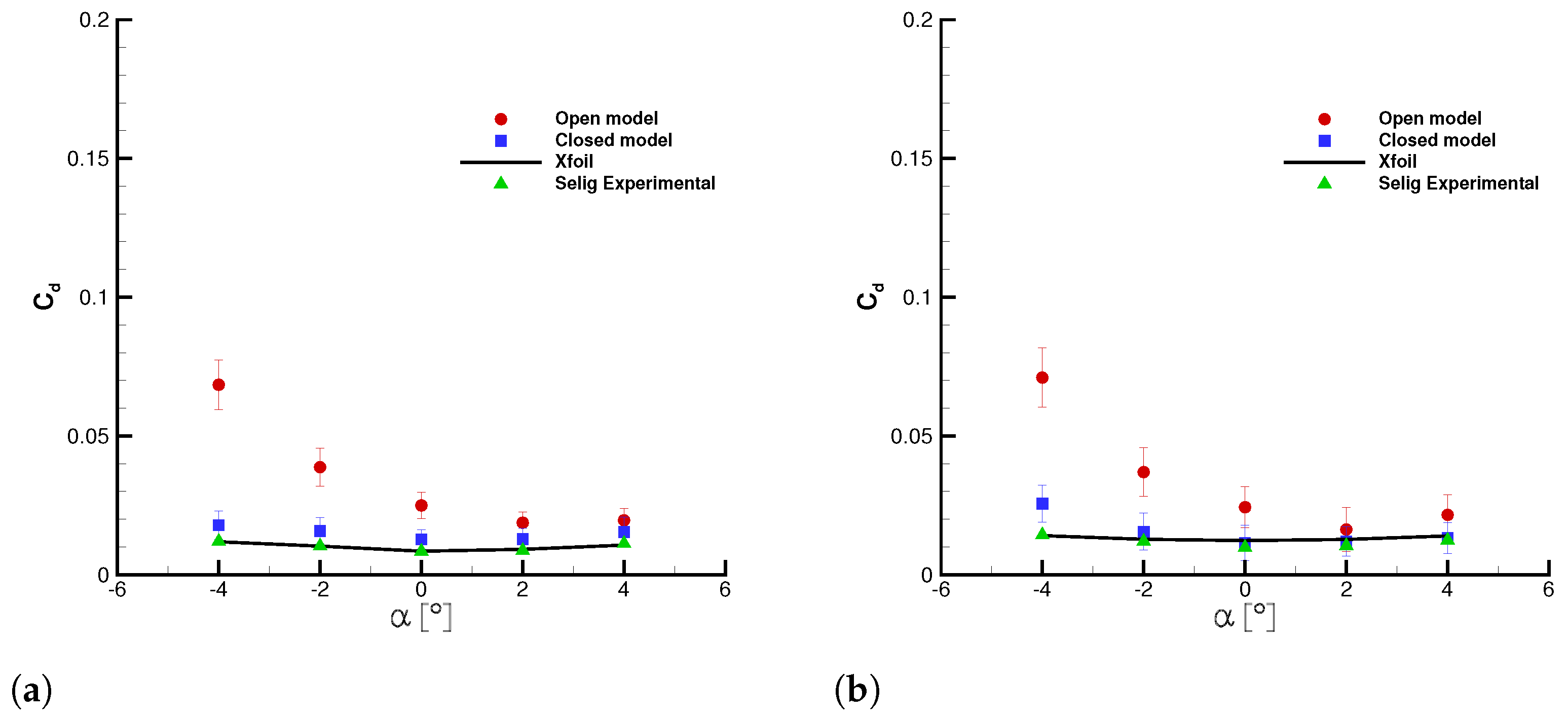
3.3. Wake Rake Analysis
The wake rake measurements were performed at angles of attack ranging from −4° to 4°.
Figure 19 and
Figure 20 show dimensionless velocity profiles in the wing wake region. The model is placed in order to align its pressure side with negative Y values on the plots. For the two Reynolds numbers, it can be observed that the wake thickness of the open wing is greater, and the minimum value of velocity is lower than the closed model. These differences are very evident at −2° and decrease at positive angles of attack.
The curves’ shape suggests a strong increase of the aerodynamic drag for the open wing, especially at negative angles of attack. This could be due to the presence of the air intake in the wing pressure side. At positive angles of attack, the difference in values is smaller because there is no discontinuity element on the suction side, and the wing is also at nearly full inflation.
The velocity distribution allows us to evaluate the drag coefficient by using the momentum equation to a control volume. The momentum loss across the wing is directly related to its aerodynamic drag.
Figure 21 shows the wing drag coefficient measured by the wake rake for the open and closed wings. The results are in good agreement with the load balance measurements.
3.4. Infrared Thermography Analysis
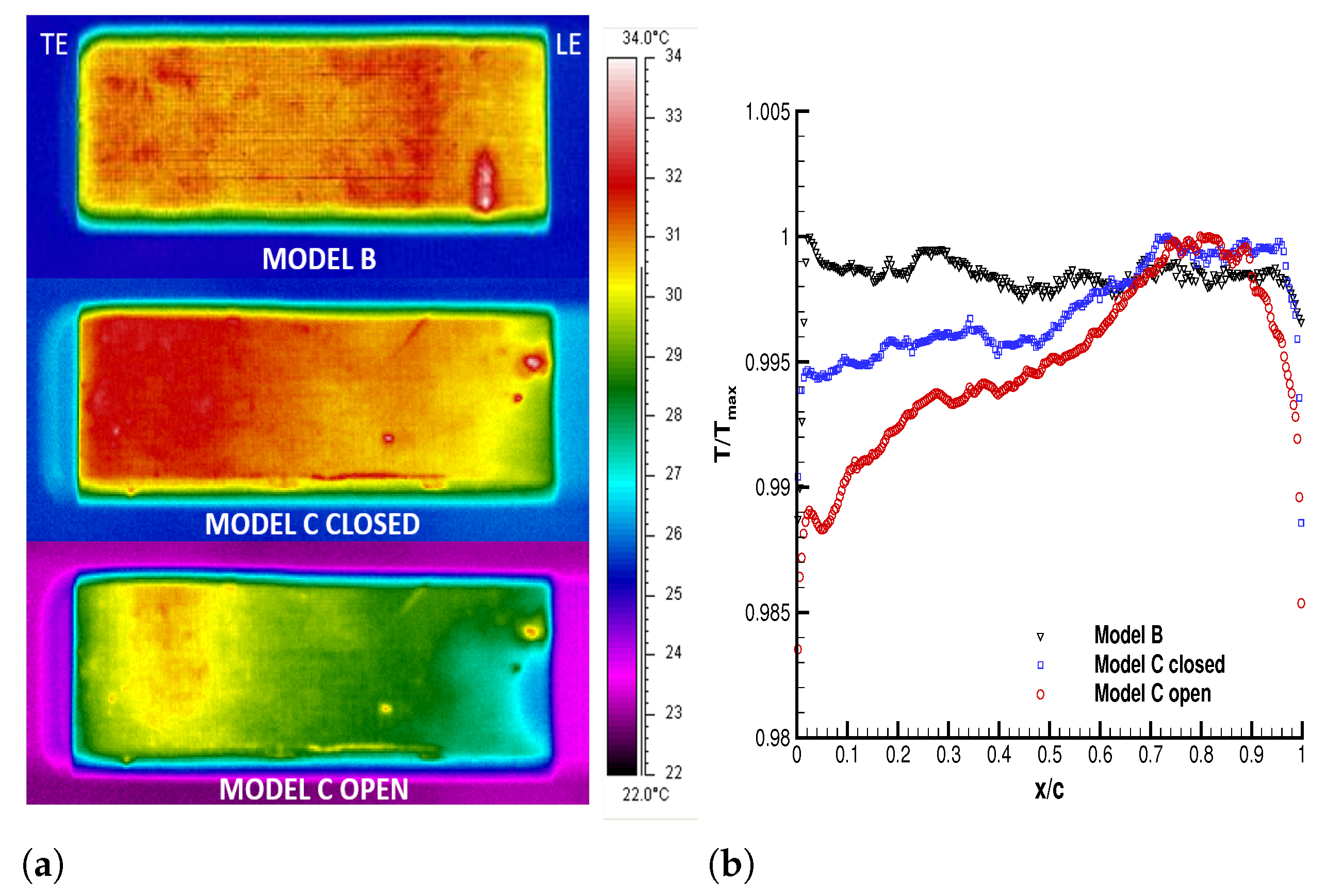
A preliminary test was performed to verify the heating uniformity of the models surface in a wind-off condition.
Figure 22 shows the thermographic images and the ratio between the local temperature and the highest temperature along the wing chord for the three tested configurations.
Model B has a strong uniformity on the wing’s suction side, which guarantees the correct functioning of the fabric as a heating source. In the two other cases (open and closed model C), a loss of uniformity can be noticed. Indeed, there is a temperature increase in the trailing edge and a decrease near the leading edge. The leading edge zone of the open wing is subjected to continuous air exchange through the air intake. The cold air inlet from the outside allows for a higher heat transfer, and the wing surface is cooled both from the inside and the outside. This effect is less effective for the closed wing because there is no air entry from outside. Instead, the trailing edge is the area with the highest temperature for both the open and closed wings. This warmer zone is due to the mutual heating between the fabric and the static air inside the wing.
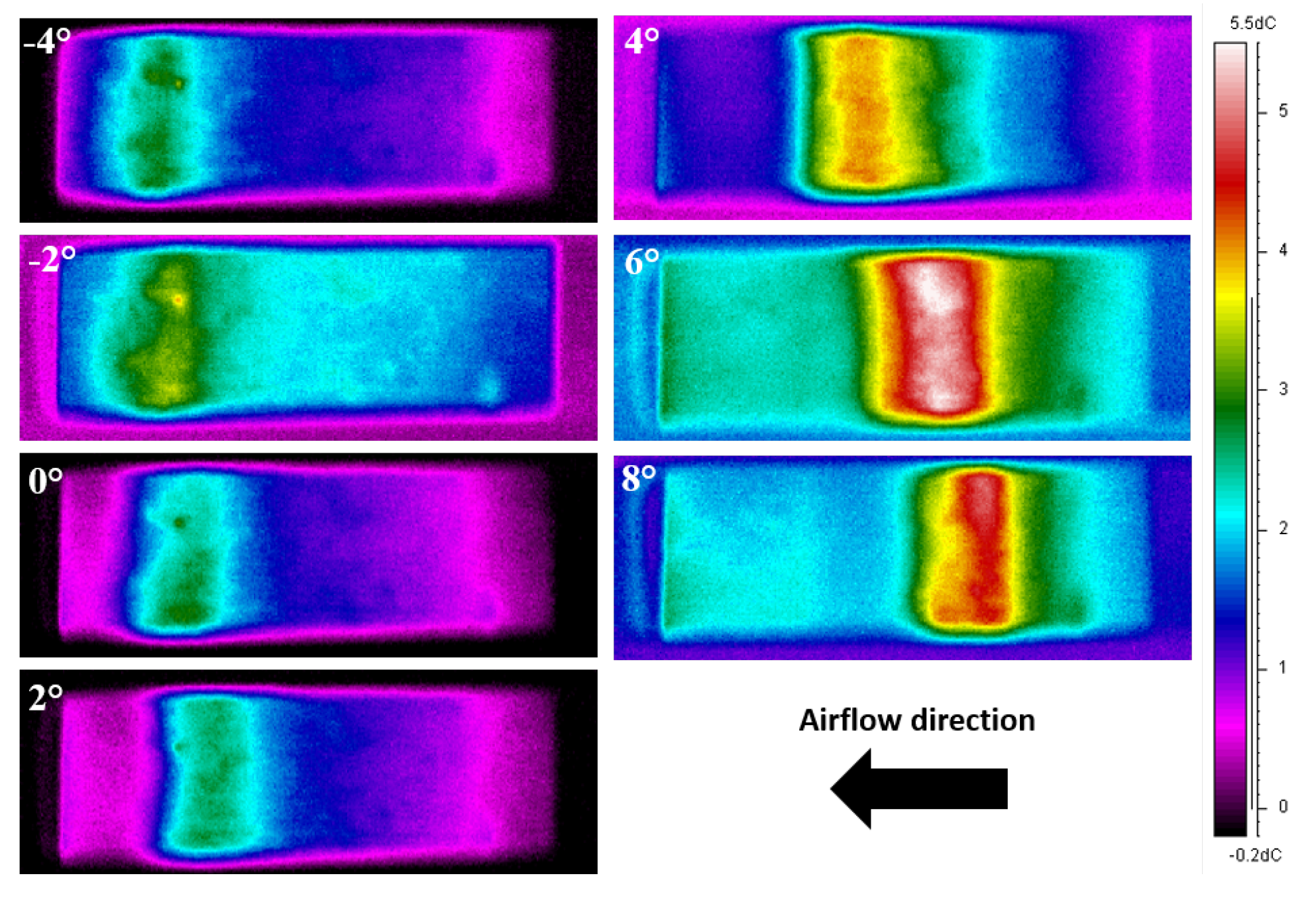
Thermographic analysis was performed for angles of attack between −4° and 8° with a step size of 2°. Only the suction side of models B and C was analyzed. Model C was tested with the air intake open and closed. For each angle of attack, a first thermographic image was acquired with the conductive layer powered. Then, a second thermographic image, obtained without electric power, was subtracted to the first one. Note that the following figures always show the temperature difference obtained between the previous acquisitions.
In
Figure 23 and
Figure 24, thermographic images of model B at Re =
and Re =
can be observed, respectively. The LSB is clearly detectable by a warmer zone in the suction side temperature distribution. It is also very noticeable that it moves from the wing’s trailing edge to the leading edge with increasing angles of attack.
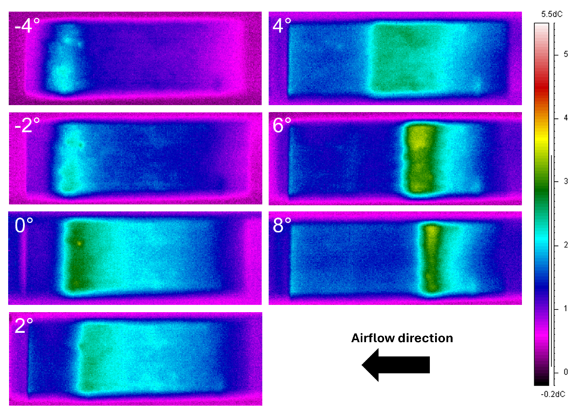
Figure 25 and
Figure 26 show the results for model C closed configuration for Re =
and Re =
, respectively. From the thermographic images, it can be noted that the temperature uniformity along the span direction was lower than that of model B. The LSB was detectable up to 4°, and its position and extension were similar to those for model B. However, the temperature non-uniformity does not allow a quantitative analysis of the LSB. At
= 6°, the higher temperature area was placed in the same position as model B only for the zone near the wooden rib. In this zone, the fabric is more rigid and less subjected to deformations. It is also important to note that this warmer zone moves toward the leading edge in unconstrained zones. This effect is related to the construction features of the leading edge of the wing. Indeed, between each pair of consecutive ribs, a balsa reinforcement was included (
Figure 5). This element creates a geometric discontinuity to the airflow.
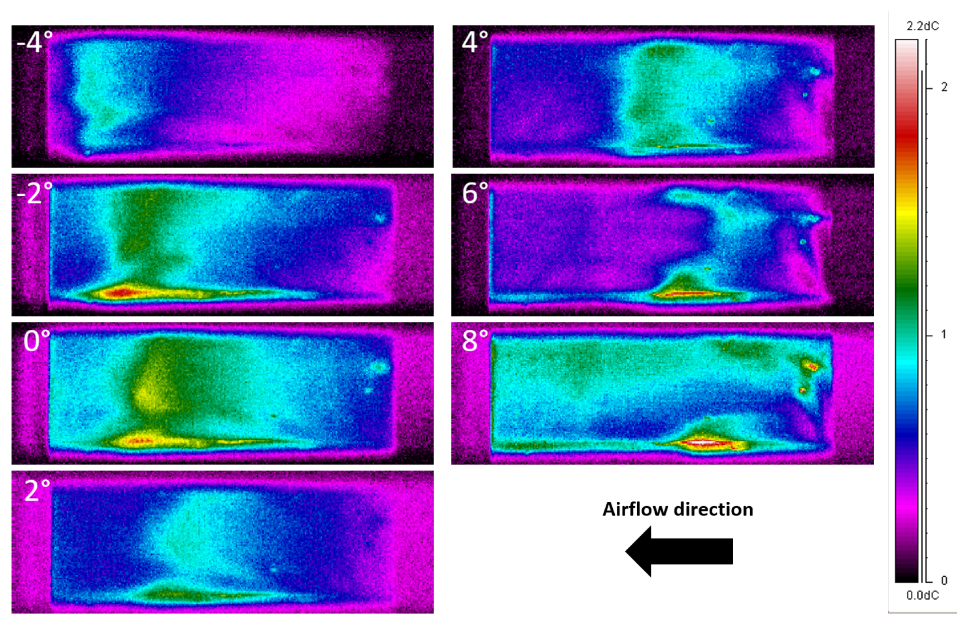
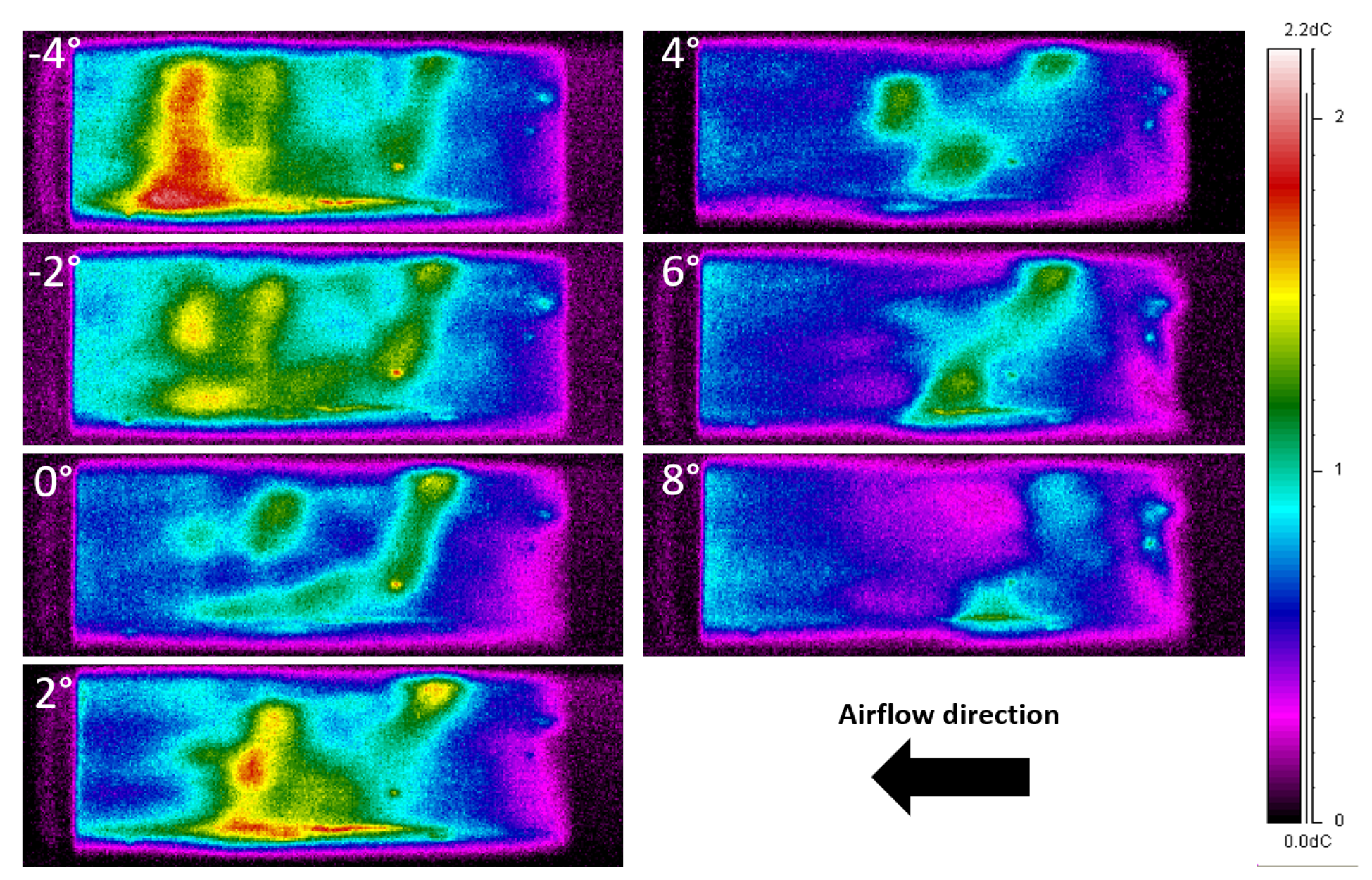
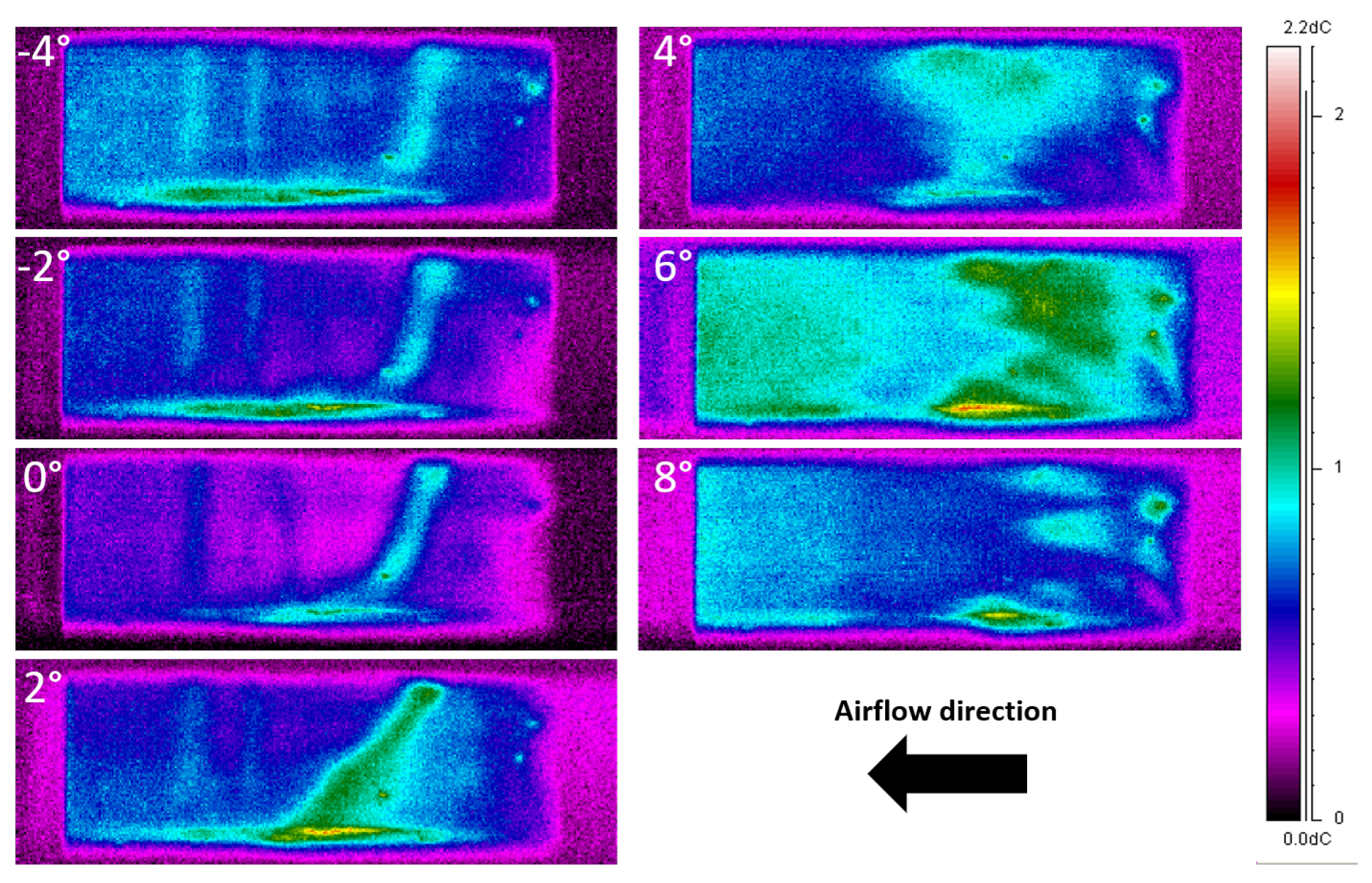
Figure 27 and
Figure 28 show the results for model C open, for Re =
and Re =
. The temperature uniformity is reduced, and the LSB is no longer detectable. However, the results put in evidence that the temperature distribution is strictly related to the fabric deformations: a local deflation in the wing surface corresponds to a greater temperature value in the thermographic image.
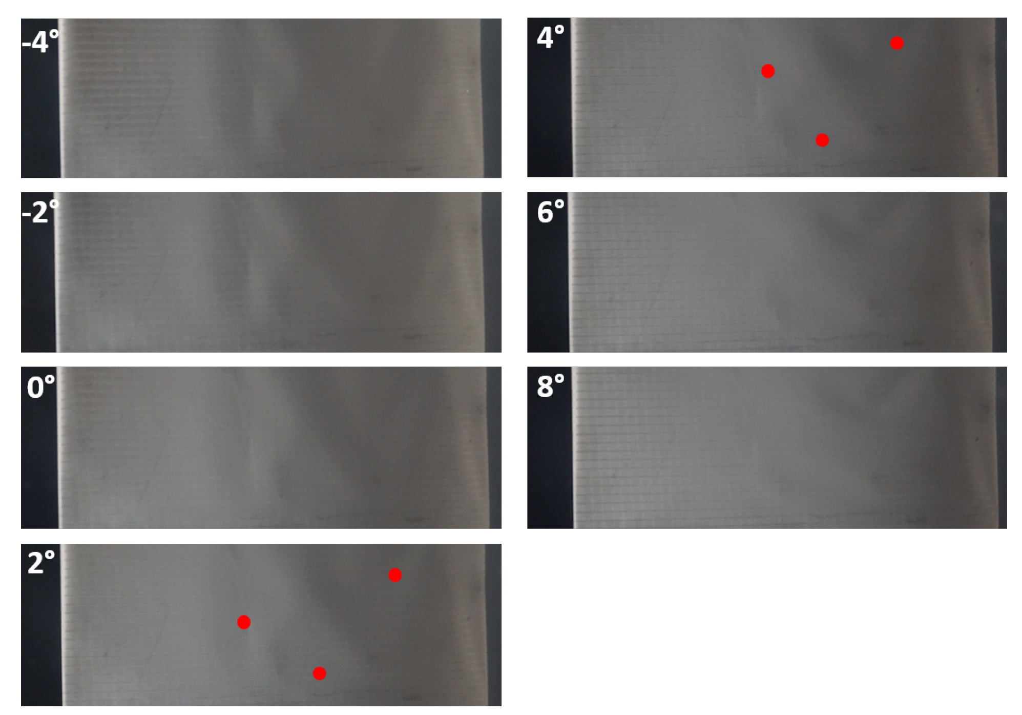
Figure 29 and
Figure 30 show the photographic images of the wing suction side at the angles of attack indicated on the figure itself, respectively, for Re =
and Re =
. Looking at the Re =
case, a higher temperature in the thermographic images corresponds to a local deflation zone on the photographic images. This is particularly clear for angles of attack equal to 2° and 4° (highlighted by red dots in
Figure 29). Furthermore, for Re =
this is even more evident since there is a higher fabric deformation. From −4° to 2° there are two vertical lines (highlighted in green in
Figure 30) in the photographic image that correspond to two lines of higher temperature in the thermographic image. These two zones are placed immediately after the rods of the model structure; from the image, it can be easily seen that the model is deflated and the fabric is pressed against the rigid structure. At this Re and
= −4°, there is an almost vertical line placed about 20% of the wing chord in the thermographic image. For higher angles of attack, this line seems to increase its slope, keeping its initial point position unchanged. Looking at the corresponding photographic image, it can be find another zone locally deflated with the same behavior, highlighted by a red line in
Figure 30. These fabric deformations disappear in the thermographic and photographic image at
= 4° when the suction side of the model inflates. From the above considerations, the fabric deformations and the temperature distribution are correlated. In fact, the surface deformations create some zones that the flow can not properly follow. This condition induces undesired boundary layer local separation and an increase of local temperature. It is interesting to note that the open configuration of model C shows the similar behavior of the closed one when it is totally inflated. Finally, the effect induced by the balsa reinforcement is clearly evident also in this case for an angle of attack of 8° and Re =
.
4. Conclusions
In this paper, the surface deformations of an inflatable wing were qualitatively investigated by infrared thermography and piezoelectric sensing. The first makes it possible to achieve a qualitative map of local deformations over a wing’s surface, while the second is able to detect the inflation/deflation phases of the wing. These deformations were correlated with aerodynamic performance and boundary layer separation phenomena investigated at Re = and Re = by means of wind tunnel experimental tests. Both the open and closed wings sections were evaluated for the sake of comparison.
The results showed that the inflatable wing presented lower lift and higher drag than the rigid one due to the fabric deformations. The open model always exhibited a higher than the closed wing; this was even more evident at negative angles of attack, where the air intake makes a significant contribution. Indeed, wake rake measurements showed a thicker wake at negative angles, while the difference decreased for positive angles of attack. The measurements point to a strong correlation between aerodynamic performance and wing inflation. Specifically, when the wing inflates, there is a change in the – slope and a drop in the coefficient, which becomes less negative.
The LSB was not clearly detectable in the inflatable model, especially for the open wing. Indeed, the temperature distribution was non-uniform and strongly affected by fabric deformations. However, these tests showed a strong interaction between the temperature distribution and the fabric deformations. Indeed, local wing deflation produced a higher-temperature zone clearly detectable in the thermographic images. The increase in temperature was caused by a convex zone corresponding to the local deflation of the wing surface. In these zones, the airflow was subjected to undesirable boundary layer separation phenomena or to a velocity decrease induced by surface curvature. In both cases, the convective heat transfer was lower. The results demonstrate the feasibility of thermographic approaches in detecting local deformations of an inflatable wing’s surface.
The results presented in this paper also confirm the feasibility of piezoelectric measurements for detecting with precision the inflation or deflation phase of a wing.
Author Contributions
Conceptualization, L.G., V.D., M.F. and R.R.; methodology, L.G., V.D., M.F. and R.R.; formal analysis, L.G., V.D., M.F. and R.R.; investigation, L.G., V.D., M.F. and R.R.; data curation, L.G., V.D., M.F. and R.R.; writing—original draft preparation, L.G., V.D., M.F. and R.R.; visualization, L.G., V.D., M.F. and R.R.; supervision, L.G., V.D., M.F. and R.R. All authors have read and agreed to the published version of the manuscript.
Funding
This research received no external funding.
Institutional Review Board Statement
Not applicable.
Data Availability Statement
The raw data supporting the conclusions of this article will be made available by the authors on request.
Conflicts of Interest
The authors declare no conflicts of interest.
References
- Burk, S.M.; Ware, G.M. Static aerodynamic characteristics of three Ram-Air inflated low aspect ratio wing. In NASA Technical Note; D-4182; NASA: Washington, DC, USA, 1967. [Google Scholar]
- Hassell, J.L., Jr.; Ware, G.M. Wind tunnel investigation of Ram-Air-Inflated all-flaxible wings of aspect ratio 1.0 to 3.0. In NASA Technical Memorandum; SX-1923; NASA: Washington, DC, USA, 1969. [Google Scholar]
- Nicolaides, J.D. Parafoil Wind tunnel test. Technical Report. AFFDL-TR-70-146. 1971. Available online: https://apps.dtic.mil/sti/tr/pdf/AD0731564.pdf (accessed on 6 January 2025).
- Mittal, S.; Saxena, P.; Singh, A. Computation of two-dimensional flows past ram-air parachutes. Int. J. Numer. Methods Fluids 2001, 35, 643–667. [Google Scholar]
- Mohammad, A.M.; Johari, H. Computation of Flow over a High Performance Parafoil. In Proceedings of the 20th AIAA Aerodynamic Decelerator Systems Technology Conference, Seattle, WA, USA, 4–7 May 2009. [Google Scholar]
- Ross, J.C. Computational Aerodynamics in the Design and Analysis of Ram-Air-Inflated Wings. In Proceedings of the 12th AIAA Aerodynamic Decelerator Systems Technology Conference, London, UK, 10–13 May 1993. [Google Scholar]
- Kenneth, J.D.; Bergeron, K.; Nyren, D.; Johari, H. Aerodynamic Investigations of a Ram-Air Parachute Canopy and an Airdrop System. In Proceedings of the 23rd AIAA Aerodynamic Decelerator Systems Technology Conference, Daytona Beach, FL, USA, 30 March–2 April 2015. [Google Scholar]
- Matos, C.; Mahalingam, R.; Ottinger, G.; Klapper, J.; Funk, R.; Komerath, N. Wind tunnel measurements of parafoil geometry and aerodynamics. In Proceedings of the 36th AIAA Aerospace Sciences Meeting and Exhibit, Reno, NV, USA, 12–15 January 1998. [Google Scholar]
- Potvin, J.; Peek, G.; Brocato, B. Modeling the Inflation of Ram-Air Parachutes Reefed with Sliders. J. Aircr. 2001, 38, 818–827. [Google Scholar] [CrossRef]
- Carruthers, A.C.; Filippone, A. Aerodynamic Drag of Parafoils. J. Aircr. 2005, 42, 1081–1083. [Google Scholar] [CrossRef]
- Lingard, J.S. Precision aerial delivery seminar, Ram-Air Parachute design. In Proceedings of the 13th AIAA Aerodynamic Decelerator Systems Technology Conference, Clearwater Beach, FL, USA, 15–18 May 1995. [Google Scholar]
- Belloc, H. Wind tunnel investigation of a rigid paraglider reference wing. J. Aircr. 2015, 52, 703–708. [Google Scholar] [CrossRef]
- Mashud, M.; Umemura, A. Experimental investigation on aerodynamic characteristics of Paraglider wing. Trans. Jpn. Soc. Aeronaut. Space Sci. 2006, 49, 9–17. [Google Scholar]
- Belloc, H.; Chapin, V.; Manara, F.; Sgarbossa, F.; Forsting, A.M. Influence of the air inlet configuration on the performances of a paraglider open airfoil. Int. J. Aerodyn. 2016, 5, 83–104. [Google Scholar]
- Boffadossi, M.; Savorgnan, F. Analysis on Aerodynamic Characteristics of a Paraglider Airfoil. Aerotec. Missili Spaz. 2016, 95, 211–218. [Google Scholar] [CrossRef]
- Abdelqodus, A.A.; Kursakov, I.A. Optimal Aerodynamic Shape Optimization of a Paraglider Airfoil Based on the Sharknose Concept. MATEC Web Conf. 2018, 221, 05002. [Google Scholar] [CrossRef]
- Hanke, K.; Schenk, S. Evaluating the geometric shape of a flying paraglider. Int. Arch. Photogramm. Remote Sens. Spatial Inf. Sci. 2014, 40, 265–272. [Google Scholar]
- Montelpare, S.; Ricci, R. A thermographic method to evaluate the local boundary layer separation phenomena on aerodynamic bodies operating at low Reynolds number. Int. J. Therm. Sci. 2004, 43, 315–329. [Google Scholar] [CrossRef]
- Astarita, T.; Cardone, G.; Carlomagno, G.M.; Meola, C. A survey on infrared thermography for convective heat transfer measurements. Opt. Laser Technol. 2000, 32, 593–610. [Google Scholar] [CrossRef]
- Astarita, T.; Cardone, G.; Carlomagno, G.M. Infrared thermography: An optical method in heat transfer and fluid flow visualisation. Opt. Lasers Eng. 2006, 44, 261–281. [Google Scholar]
- Ricci, R.; Montelpare, S. A quantitative IR thermographic method to study the laminar separation bubble phenomenon. Int. J. Therm. Sci. 2005, 44, 709–719. [Google Scholar]
- Barlow, J.B.; Rae, W.H., Jr.; Pope, A. Low-Speed Wind Tunnel Testing, 3rd ed.; Wiley: Hoboken, NJ, USA, 1999. [Google Scholar]
- Selig, M.S.; Donovan, J.F.; Fraser, D.B. Airfoil at Low Speeds, 1st ed.; H.A. Stokely: Virginia Beach, VA, USA, 1989. [Google Scholar]
Figure 1.
The subsonic wind tunnel of Università Politecnica delle Marche.
Figure 1.
The subsonic wind tunnel of Università Politecnica delle Marche.
Figure 2.
View factors of the suction sides of the wing and of a flat plate.
Figure 2.
View factors of the suction sides of the wing and of a flat plate.
Figure 3.
Positioning of hot points: (a) wing’s leading edge and (b) wing’s trailing edge.
Figure 3.
Positioning of hot points: (a) wing’s leading edge and (b) wing’s trailing edge.
Figure 4.
Model A: (a) pressure and suction side and (b) detail of the piezoelectric sensor’s position.
Figure 4.
Model A: (a) pressure and suction side and (b) detail of the piezoelectric sensor’s position.
Figure 5.
Models for thermographic tests: (a) model C, (b) model B, and (c) model C intake detail.
Figure 5.
Models for thermographic tests: (a) model C, (b) model B, and (c) model C intake detail.
Figure 6.
Piezoelectric signal: (a) signal not filtered and (b) signal filtered at 10 Hz.
Figure 6.
Piezoelectric signal: (a) signal not filtered and (b) signal filtered at 10 Hz.
Figure 7.
Piezoelectric signal in the wind-off condition from = 0° to = 2°.
Figure 7.
Piezoelectric signal in the wind-off condition from = 0° to = 2°.
Figure 8.
Piezoelectric signal at Re = from = −2° to = 0°.
Figure 8.
Piezoelectric signal at Re = from = −2° to = 0°.
Figure 9.
Piezoelectric signal at Re = from = 0° to = 2°.
Figure 9.
Piezoelectric signal at Re = from = 0° to = 2°.
Figure 10.
Piezoelectric signal at Re = from = 0° to = 2°.
Figure 10.
Piezoelectric signal at Re = from = 0° to = 2°.
Figure 11.
Piezoelectric signal at Re = from = 2° to = 4°.
Figure 11.
Piezoelectric signal at Re = from = 2° to = 4°.
Figure 12.
Piezoelectric signal at Re = from = 2° to = 0°.
Figure 12.
Piezoelectric signal at Re = from = 2° to = 0°.
Figure 13.
Piezoelectric signal at Re = from = 0° to = −2°.
Figure 13.
Piezoelectric signal at Re = from = 0° to = −2°.
Figure 14.
Piezoelectric signal at Re = from = 0° to = −2°.
Figure 14.
Piezoelectric signal at Re = from = 0° to = −2°.
Figure 15.
Piezoelectric signal at Re = from = −2° to = −4°.
Figure 15.
Piezoelectric signal at Re = from = −2° to = −4°.
Figure 16.
Load balance results at Re = : (a) – and (b) – curves.
Figure 16.
Load balance results at Re = : (a) – and (b) – curves.
Figure 17.
Load balance results at Re = : (a) – and (b) – curves.
Figure 17.
Load balance results at Re = : (a) – and (b) – curves.
Figure 18.
– curves: (a) Re = and (b) Re = .
Figure 18.
– curves: (a) Re = and (b) Re = .
Figure 19.
Wake rake results at Re = : (a) = −2° and (b) = 2°.
Figure 19.
Wake rake results at Re = : (a) = −2° and (b) = 2°.
Figure 20.
Wake rake results at Re = : (a) = −2° and (b) = 2°.
Figure 20.
Wake rake results at Re = : (a) = −2° and (b) = 2°.
Figure 21.
– curves: (a) Re = and (b) Re = .
Figure 21.
– curves: (a) Re = and (b) Re = .
Figure 22.
Heating uniformity test: (a) Thermographic images and (b) temperature distribution along the wing chord.
Figure 22.
Heating uniformity test: (a) Thermographic images and (b) temperature distribution along the wing chord.
Figure 23.
Thermographic images of model B at Re = .
Figure 23.
Thermographic images of model B at Re = .
Figure 24.
Thermographic images of model B at Re = .
Figure 24.
Thermographic images of model B at Re = .
Figure 25.
Thermographic images of model C closed at Re = .
Figure 25.
Thermographic images of model C closed at Re = .
Figure 26.
Thermographic images of model C closed at Re = .
Figure 26.
Thermographic images of model C closed at Re = .
Figure 27.
Thermographic images of model C open at Re = .
Figure 27.
Thermographic images of model C open at Re = .
Figure 28.
Thermographic images of model C open at Re = .
Figure 28.
Thermographic images of model C open at Re = .
Figure 29.
Photographic images of model C open at Re = .
Figure 29.
Photographic images of model C open at Re = .
Figure 30.
Photographic images of model C open at Re = .
Figure 30.
Photographic images of model C open at Re = .
Table 1.
Load balance features.
Table 1.
Load balance features.
| Channel | Full Scale | Uncertainty |
|---|
| Lift [N] | 50 | |
| Drag [N] | 20 | |
| Moment [Nm] | | |
Table 2.
Comparison of the signals acquired with the two different bandwidths.
Table 2.
Comparison of the signals acquired with the two different bandwidths.
| 200 MHz | 10 kHz |
|---|
|
Mean
|
Standard Dev.
|
Mean
|
Standard Dev.
|
|---|
| Test 1 | | | | |
| Test 2 | | | | |
| Disclaimer/Publisher’s Note: The statements, opinions and data contained in all publications are solely those of the individual author(s) and contributor(s) and not of MDPI and/or the editor(s). MDPI and/or the editor(s) disclaim responsibility for any injury to people or property resulting from any ideas, methods, instructions or products referred to in the content. |
© 2025 by the authors. Licensee MDPI, Basel, Switzerland. This article is an open access article distributed under the terms and conditions of the Creative Commons Attribution (CC BY) license (https://creativecommons.org/licenses/by/4.0/).


