Deep LBLS: Accelerated Sky Region Segmentation Using Hybrid Deep CNNs and Lattice Boltzmann Level-Set Model

Abstract

Accurate segmentation of the sky region is crucial for various applications, including object detection, tracking, and recognition, as well as augmented reality (AR) and virtual reality (VR) applications. However, sky region segmentation poses significant challenges due to complex backgrounds, varying lighting conditions, and the absence of clear edges and textures. In this paper, we present a new hybrid fast segmentation technique for the sky region that learns from object components to achieve rapid and effective segmentation while preserving precise details of the sky region. We employ Convolutional Neural Networks (CNNs) to guide the active contour and extract regions of interest. Our algorithm is implemented by leveraging three types of CNNs, namely DeepLabV3+, Fully Convolutional Network (FCN), and SegNet. Additionally, we utilize a local image fitting level-set function to characterize the region-based active contour model. Finally, the Lattice Boltzmann approach is employed to achieve rapid convergence of the level-set function. This forms a deep Lattice Boltzmann Level-Set (deep LBLS) segmentation approach that exploits deep CNN, the level-set method (LS), and the lattice Boltzmann method (LBM) for sky region separation. The performance of the proposed method is evaluated on the CamVid dataset, which contains images with a wide range of object variations due to factors such as illumination changes, shadow presence, occlusion, scale differences, and cluttered backgrounds. Experiments conducted on this dataset yield promising results in terms of computation time and the robustness of segmentation when compared to state-of-the-art methods. Our deep LBLS approach demonstrates better performance, with an improvement in mean recall value reaching up to 14.45%.

1. Introduction

In applications such as object detection, tracking, and recognition, precisely segmenting the sky region is essential for understanding the scene’s context and environment [1,2]. Separating the sky region provides a distinctive visual cue that can assist in categorizing and organizing images based on their sky characteristics. This enables efficient retrieval of images containing specific sky types or scenes, which is mainly used for image retrieval and indexing systems [3,4]. Moreover, in augmented reality (AR) and virtual reality (VR) applications, accurate sky region segmentation is essential for realistic scene rendering [5,6]. By accurately separating the sky, virtual objects or effects can be seamlessly integrated into the sky region, enhancing the overall visual quality and realism of the augmented or virtual environment.

The field of image segmentation has witnessed a significant surge in interest, particularly in the subclass of sky region segmentation. This particular area of research has garnered extensive attention, driven by the growing demand for accurate and efficient detection of objects in the sky, especially in the context of aerial surveillance, drone navigation, satellite imaging, and military applications [7]. The sky region often exhibits complex and variable background patterns, such as clouds, gradients, and atmospheric effects. These variations make it difficult to define a consistent boundary for the sky region. Unlike many other objects or regions in an image, the sky region often lacks clear edges and distinct texture. This absence of prominent features makes it challenging to identify the boundaries of the sky region accurately. The color and intensity distribution of the sky region can overlap with other regions in the image, such as buildings, mountains, or water bodies. This similarity in color and intensity makes it challenging to differentiate the sky region from its surroundings. The sky region is highly sensitive to lighting conditions, resulting in significant variations in illumination throughout the day and under different weather conditions. Additionally, shadows from objects in the scene can further complicate the segmentation process by altering the appearance and boundaries of the sky region. In many outdoor scenes, objects such as trees, buildings, or mountains can partially or fully occlude the sky region. These occlusions and overlapping objects introduce additional complexity to the segmentation task as they can interfere with the accurate delineation of the sky region.

Thus, addressing these challenges requires the development of sophisticated algorithms and techniques that can handle complex backgrounds, handle variations in color and texture, account for illumination changes and shadows, handle occlusions and overlapping objects, and adapt to scale and perspective variations. Research has been continuously conducted to advance image processing methods, overcome challenges, and improve the accuracy and robustness of region segmentation [8,9].

Machine learning and deep learning have proven to be powerful techniques for image segmentation and classification applications [10,11,12,13]. One widely adopted deep learning method for image segmentation involves the application of Convolutional Neural Networks (CNNs). These networks are particularly effective at capturing spatial information within images, making them well-suited for segmentation tasks [14]. They are effective in capturing spatial information through convolutional layers and can learn hierarchical representations from input images. Several extension architectures to the CNN are commonly used for image segmentation, including U-Nets, Fully Convolutional Networks (FCNs) [15], and SegNet [16]. These architectures typically consist of an encoder part that captures the features from the input image and a decoder part that upsamples the features to generate the segmentation map. CNNs can handle complex image structures and capture both local and global contextual information. They can learn powerful feature representations through a deep architecture. Moreover, CNNs can be trained end-to-end, allowing for efficient optimization. Several approaches have been proposed to address the challenges of region segmentation with deep learning in image processing. Hasenbalg et al. [1] emphasized the importance of accurate sky region segmentation in applications like object detection, tracking, and recognition. They provided a benchmark for evaluating various segmentation methods, highlighting the need for robust techniques in the presence of extreme variations in illumination, shadow, occlusion, scale, and clutter. In image retrieval and indexing systems, researchers have explored several methods for efficiently categorizing and organizing images based on their sky characteristics [2,3,4]. The focus of this paper is on the precise segmentation of the sky region, crucial for such applications.

Han et al. [17] proposed a deep level-set method that combines deep learning techniques with the level-set method. The deep level-set method aims to improve the accuracy and efficiency of image segmentation by incorporating learned priors from FCN neural networks. However, their work cannot achieve the required segmentation output when the scene is more complex and contains clutter. Additionally, the paper does not address the execution time.

Zheng et al. [18] introduced a combination of deep learning and the level-set method for image segmentation. They present a deep learning framework that incorporates level-set evolution into the loss function, enabling simultaneous learning of image features and level-set evolution for accurate segmentation.

Moreover, Albalooshi et al. [19] emphasize the significance of utilizing an unsupervised pre-trained deep neural network to guide the evolution of active contour segmentation for object segmentation. Their approach capitalizes on the learned representations from the deep neural network, enabling their algorithm to effectively capture and exploit the unique features associated with objects of interest. By incorporating these distinctive features, the accuracy of the segmentation process is greatly enhanced, leading to more precise and reliable results. Their work highlights the importance of leveraging the power of deep neural networks. Through unsupervised pre-training, the deep neural network can autonomously learn relevant features from a large dataset, enabling it to effectively guide the active contour evolution. This approach addresses the challenge of accurately identifying and segmenting objects, which often exhibit complex patterns and textures that require sophisticated analysis.

Liu et al. [20] proposed a hybrid deep learning with a Lattice Boltzmann method (LBM) framework for rapid image segmentation. However, their method does not adequately consider noise and artifacts presented in the input images. When the input images contain significant levels of noise or artifacts, the segmentation accuracy may be adversely affected, leading to inaccurate boundaries.

In a study carried out by Singh et al. [21], Convolutional Neural Networks (CNNs) were employed to segment and discriminate cotton boll pixels from sky pixels. Three fully convolutional neural network models (VGG16 [22], InceptionV3 [23], and ResNet34 [24]) were used as encoders and trained on a dataset. The trained models were evaluated using evaluation metrics such as intersection-over-union (IoU), F1-score, precision, and recall deployed in cotton harvesting applications.

The sky view factor (SVF) has gained recognition as an important indicator for evaluating the openness of streets in urban planning [25]. It quantifies the ratio of visible sky area to the total sky area at a specific point in space. With the availability of street view images (SVIs) and the emergence of SVI services providing panoramic data of urban street levels, Xia et al. [25] developed a method to measure street-level SVF by leveraging semantic segmentation techniques to extract sky area data from SVIs. This enabled the estimation of the fisheye photographic-based sky view factor (SVFf).

Accordingly, deep learning and the lattice Boltzmann level-set method are two distinct approaches that have been used in various image segmentation applications. However, the combination of these two techniques has not been addressed very well in the context of sky region segmentation. To the best of our knowledge, there is no specific solution that combines CNNs with a lattice Boltzmann level-set approach for segmentation in all-sky images. Thus, in this paper, we introduce a hybrid approach by integrating CNNs and the lattice Boltzmann level-set method, highlighting our contributions, challenges, and applications.

We benchmark our model against leading CNN-based segmentation models, including DeepLabV3+, FCNs, and SegNet. This selection is based on several key factors, including their proven effectiveness in semantic segmentation tasks, their architectural advantages, and their relevance to the challenges associated with sky region segmentation. The ability of DeepLabV3+ to handle multi-scale features and preserve spatial resolution makes it particularly suitable for sky region segmentation, where the sky often lacks clear edges and textures, and its appearance can vary significantly due to lighting conditions, occlusions, and atmospheric effects. FCNs incorporate skip connections that fuse feature maps from different layers of the network. This helps preserve fine-grained details by combining low-level features (e.g., edges) with high-level semantic information, which is particularly useful for segmenting the sky region, where subtle gradients and color variations are common. SegNet is computationally efficient and can handle large images, making it suitable for real-time applications such as drone navigation or aerial surveillance, where sky region segmentation is often required. SegNet’s ability to handle complex scenes with occlusions and overlapping objects aligns well with the challenges of sky region segmentation, where objects like trees, buildings, or mountains may partially occlude the sky. By selecting these three models, we aimed to provide a comprehensive comparison of different segmentation approaches. All three models are suited to address the specific challenges of sky region segmentation, such as complex backgrounds, varying lighting conditions, and the absence of clear edges.

Table 1. Summary comparison with existing methods.

Method	Advantages	Disadvantages	Our Contribution (Deep LBLS)
DeepLabV3+ [26]	High accuracy in semantic segmentation	Computationally intensive	Combines DeepLabV3+ with LBLS for improved boundary detection
	Multi-scale feature aggregation	limited ability to handle complex boundaries	Faster convergence with LBM
FCN [27]	End-to-end training	Struggles with fine details	Enhances FCN with LBLS for better object completeness and boundary smoothness
	Preserves spatial resolution	Limited contextual understanding
SegNet [16]	Simple encoder-decoder architecture	Limited feature extraction capabilities	Improves SegNet’s performance with LBLS, especially in handling occlusions and complex skies
	Easy to train	Lower accuracy in complex scenes
Level-Set Methods [17,18]	Effective for boundary evolution	Computationally expensive	Integrates level-set with LBM for faster convergence and reduced computational cost
	Handles topological changes	Sensitive to initialization
Lattice Boltzmann Methods [20]	Efficient for fluid dynamics and boundary tracking	Limited application in image segmentation	Combines LBM with deep learning for accurate and efficient sky region segmentation
	Parallelizable	Requires careful parameter tuning

summarizes the key differences, advantages, and disadvantages of our proposed method compared to existing approaches.

In the context of aerial surveillance using drones, accurate segmentation of the sky region is crucial for various tasks such as object detection, scene understanding, and anomaly detection. By integrating the Deep LBLS approach into the image processing pipeline of the aerial surveillance system, the system can focus on identifying objects of interest against the sky background, enhancing surveillance capabilities. Moreover, the segmented sky region can serve as a reference point for anomaly detection. Unusual activities or objects in the sky, such as unauthorized drones or aircraft, can be easily identified against the segmented sky background, triggering timely alerts. Additionally, segmentation of the sky region can aid in drone navigation and collision avoidance. By accurately delineating the sky area, drones can better navigate through complex environments and avoid collisions with obstacles or other airborne objects.

Our proposed method combines CNN techniques with the lattice Boltzmann level-set approach, aiming to enhance accuracy, processing efficiency, and robustness to variations in sky appearance, lighting conditions, and complex backgrounds. In the subsequent sections, we provide a detailed description of our proposed deep LBLS method.

Hence, we introduce a new method for segmenting the sky region in images using a combination of deep learning and the lattice Boltzmann level-set approach. Our contributions in this research are:

• Improved Accuracy: By integrating deep learning techniques with the lattice Boltzmann level-set approach, our goal is to surpass the precision and reliability of conventional segmentation methods, resulting in more accurate delineation of sky regions.
• Efficient Computational Process: We present a method that achieves a balance between computational efficiency and prediction accuracy in sky region segmentation. Deep learning algorithms are often computationally intensive, however, the incorporation of the lattice Boltzmann level-set approach mitigates this, offering an effective solution.
• Robustness to Variations: Our method addresses the challenges posed by diverse sky appearances, varying lighting conditions, and complex backgrounds. The proposed framework is capable of learning intricate patterns and features, enabling the system to adjust to different sky scenarios.
• Integration of Lattice Boltzmann Level-Set: We incorporate the lattice Boltzmann level-set approach into the deep CNNs framework to provide additional advantages. The lattice Boltzmann method is adept at tackling dynamic boundaries and evolving shapes, which aids in achieving more precise and smoother segmentation outcomes for sky regions.

The rest of the article is organized as follows. Section 2 illustrates the proposed deep Lattice Boltzmann Level-Set (deep LBLS) model. Results and discussions are discussed in Section 3. Finally, Section 4 presents our conclusions and future directions.

2. Materials and Methods

This section introduces our fast and robust sky region segmentation approach. We’ll begin with a general outline of the method, followed by an in-depth exploration of each step.

2.1. Outline of the Key Steps in the Proposed Technique

Our segmentation approach integrates deep CNN within the level-set image fitting for accurate boundary and region extraction of the sky region. Additionally, the proposed method incorporates the LBM to reduce computational time. A functional framework of the proposed segmentation is illustrated in Figure 1, which is based on four algorithmic steps. The first step involves using dense feature maps to cluster the intensity information of the sky region by leveraging a supervised CNN model. The input of the deeply learned neural networks is then employed in the second stage of our segmentation process to map the intensity levels of an input-testing image. The mapped output values are subsequently utilized to evolve the energy function of the level-set protocol in the third stage of our proposed approach. Finally, the LBM is used to solve the curve evolution problem and optimize the convergence of the contour to the most optimum sky region boundaries.

2.2. Deep Learning Based Sky Region Segmentation

We utilize deep CNNs for semantic segmentation of the sky region as a first step. This phase involves training a deep neural network to learn the features and patterns in the image data about the sky region and then performing those features to make predictions about the location and boundaries of the sky region in our testing imagery. During the training phase, we utilize the Cambridge-driving Labelled Video Database (CamVid) [28], because it consists of images containing the sky region along with corresponding ground truth segmentation masks. These segmentation masks have pixel-level annotations that indicate which regions belong to the sky area. The dataset encompasses a diverse range of outdoor images with various lighting conditions, occlusions, and backgrounds.

To enhance the dataset for optimal neural network performance, we standardize the image dimensions to a uniform resolution and adjust the pixel values for normalization, aligning with the specifications of the deep learning model utilized. Image augmentation techniques are employed to enrich the training dataset’s variety, thereby boosting the model’s performance. This is achieved through the application of random transformations to the training images throughout the training process.

The dataset is partitioned into three subsets: 421 images for training, 140 images for validating, and 140 images for testing. In the training phase, the network is supplied with the input images alongside their respective ground truth segmentation masks, enabling it to learn the mapping from input to accurate segmentation outputs. To optimize the model, adjustments are made to its parameters and weights via the Stochastic Gradient Descent (SGD) optimization technique. Furthermore, these parameters are iteratively updated to reduce the loss function, enhancing the model’s performance and accuracy.

Upon completing the training phase, we employ the previously unseen testing image set to deploy our deep neural network for the initial segmentation of the sky region during the testing phase. To comprehensively evaluate the performance of our proposed approach, we benchmark our model against leading CNN-based segmentation models, such as DeepLabV3+, FCNs, and SegNet. This comparison allows for a more nuanced understanding of how our model stands in relation to the current state-of-the-art in the field.

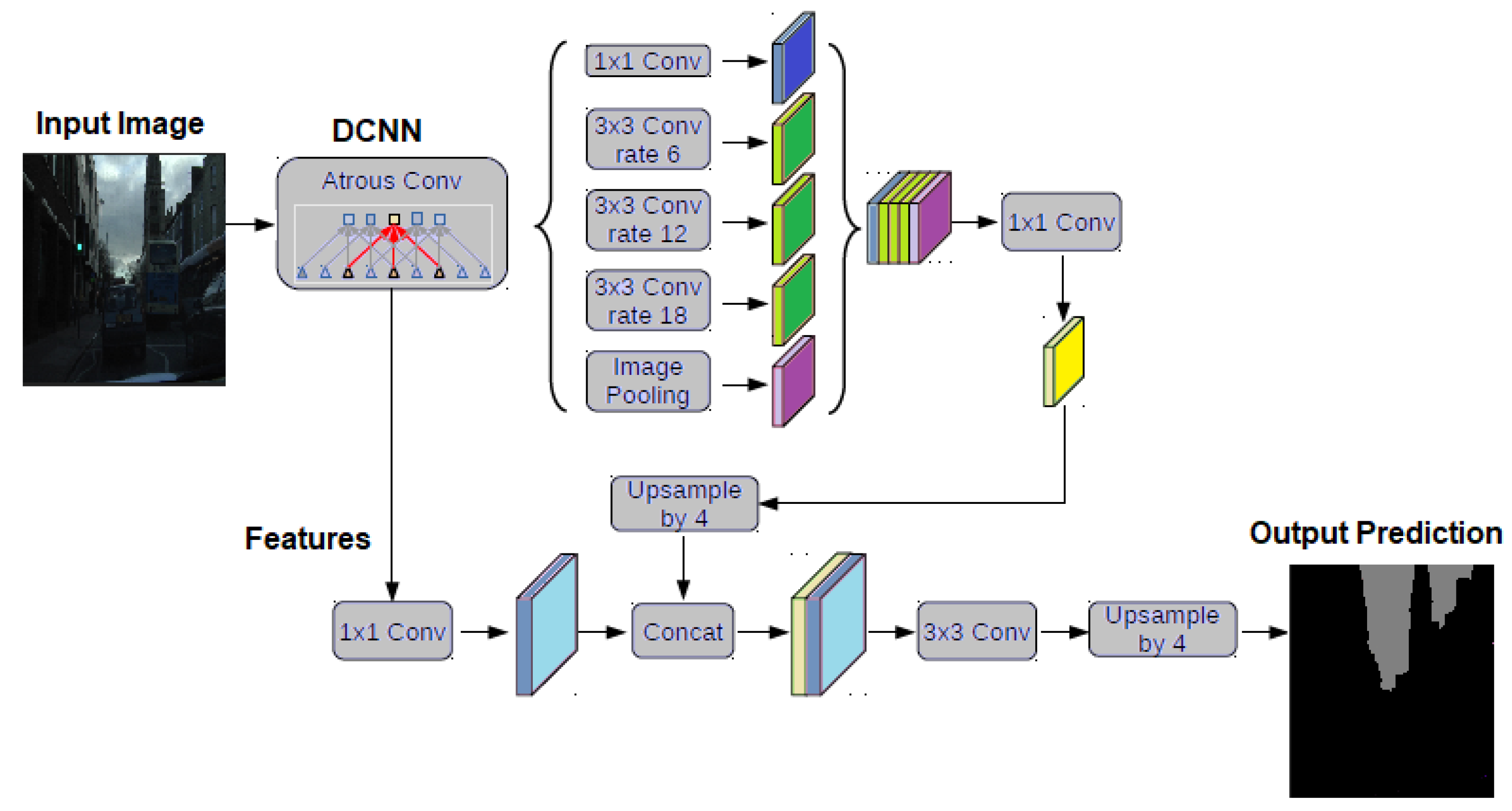
2.2.1. DeepLabV3+

DeepLabV3+ is a state-of-the-art method for semantic image segmentation [26]. It uses both atrous spatial pyramid pooling and decoder modules to enhance segmentation results. Figure 2 illustrates the structural components of the DeepLabV3+ algorithm.

In the DeepLabV3+ model, Atrous convolution is performed on the input feature map x for each location i on the output feature map y and a convolution filter w in the following manner:

$$y\left[i\right]=\sum _{k}x[i+r·k]w\left[k\right]$$

(1)

where the sampling stride of the input signal is determined by the atrous rate r that is used in the process.

DeepLabV3+ is known to use Atrous Spatial Pyramid Pooling (ASPP) [26], which prompts the feature representation for each pixel by capturing multi-scale context by sampling the input image at multiple rates. Additionally, DeepLabV3+ incorporates the Xception model and atrous separable convolution to make the model faster and more robust.

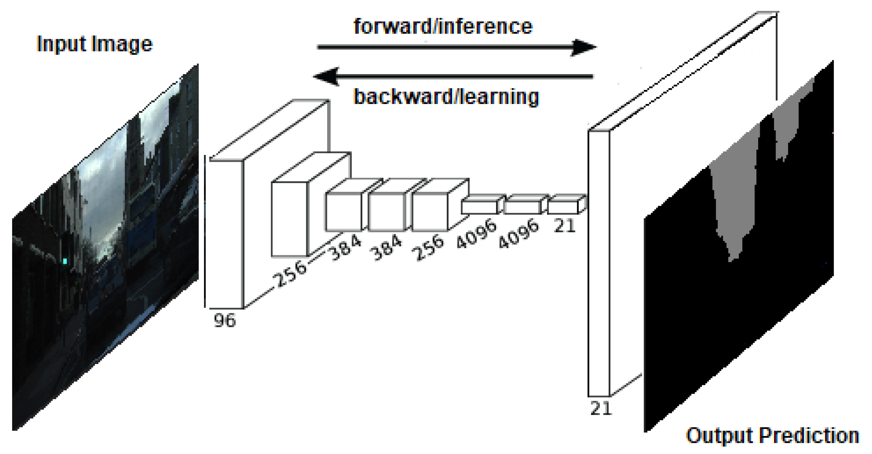
2.2.2. Fully Convolutional Networks (FCNs)

Fully Convolutional Networks (FCNs) are deep learning models designed for semantic segmentation tasks [27]. FCNs incorporate skip connections to fuse feature maps from different stages of the network. These connections help in preserving fine-grained details by combining low-level features with high-level semantic information. Moreover, FCNs employ transposed convolutions, also known as deconvolutions or upsampling layers, to recover the spatial resolution of the feature maps. Transposed convolutions increase the size of feature maps, allowing the network to generate a segmentation map with the same dimensions as the input image. FCNs can be trained in an end-to-end manner, meaning the entire network is trained jointly. The network learns to perform both feature extraction and pixel-wise classification simultaneously, optimizing the parameters of the entire model to minimize a segmentation loss function. FCNs produce dense predictions by generating a pixel-wise classification map for each input image. This means that every pixel in the input image is assigned a label or class, enabling accurate and detailed segmentation results. Figure 3 illustrates the structural components of the FCN algorithm.

Overall, FCNs belong to a powerful class of deep-learning models designed for semantic segmentation. They leverage skip connections, transposed convolutions, and end-to-end training to generate dense predictions and accurately segment objects within images. FCNs have found widespread applications in various domains, showcasing their effectiveness in pixel-level labeling tasks.

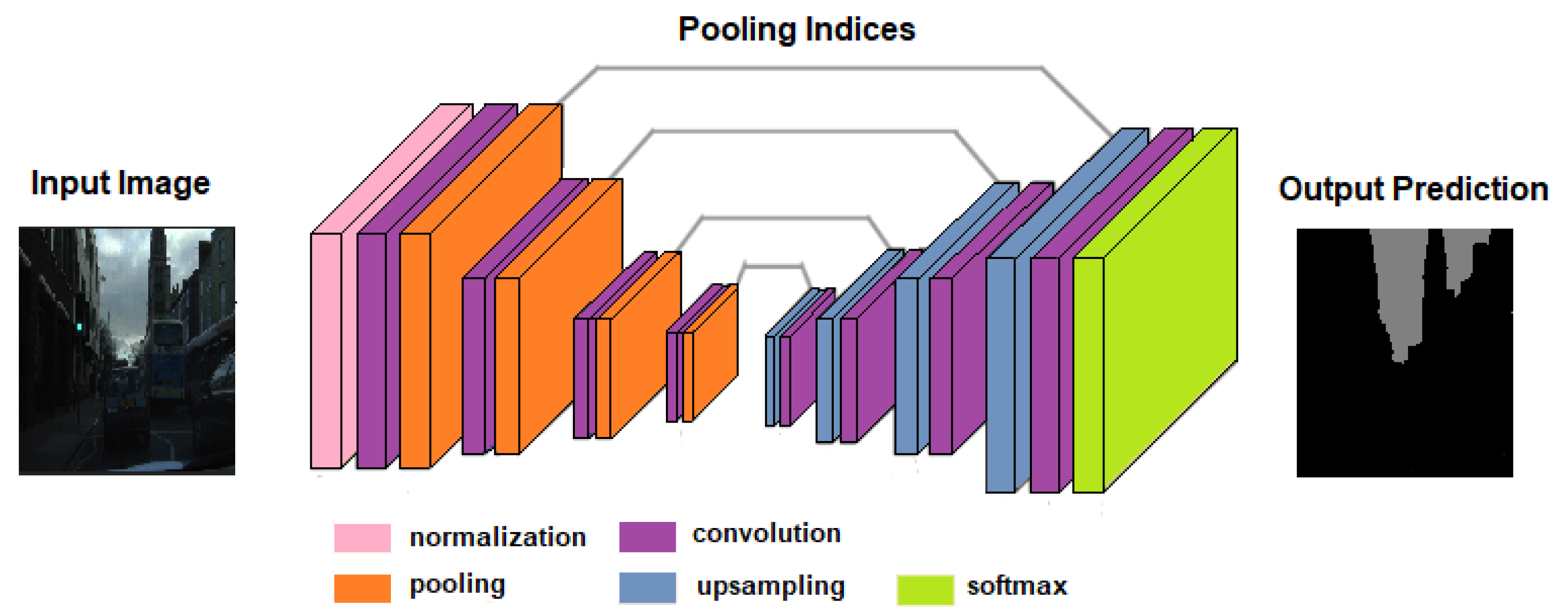
2.2.3. SegNet

SegNet [16] is a deep learning-based semantic segmentation method that uses an encoder-decoder architecture to learn the mapping between the input image and its corresponding semantic segmentation. The encoder part of the network extracts features from the input image, while the decoder part generates the segmentation mask. Figure 4 illustrates the structural components of the SegNet algorithm.

The SegNet architecture comprises three key components: the encoder, decoder, and segmentation module. The encoder extracts features from the input image while the decoder generates the segmentation mask. The segmentation module upsamples the decoder’s feature maps to produce the final segmentation mask. Training of the SegNet model involves end-to-end learning using a dataset of labeled images. During training, the model minimizes the disparity between predicted and ground truth segmentation masks, typically employing a combination of cross-entropy loss and dice loss.

Once trained, the model can perform semantic segmentation on new images. The input image undergoes encoding, generating feature maps that are then processed by the decoder to yield the segmentation mask. SegNet offers advantages over other deep learning-based semantic segmentation methods, including its capability to handle large images and produce high-quality segmentation masks. It is also relatively easy to train and can be trained with small datasets.

2.3. Evolve the Level-Set Energy Function

The level-set method is a mathematical framework for tracking the evolving interfaces and contours. This method represents the interface as the zero contour of a higher-dimensional level-set function and evolves it over time using partial differential equations. The evolution of this level-set function adheres to an equation that minimizes a cost function, typically incorporating terms associated with data fidelity and regularization.

We employ a variational level-set approach, where the contour C is defined by the zero level-set of an auxiliary functional denoted as $\phi (x,y,t)$ or simply $\phi$. The evolution of $\phi$ can be described by the following equation:

$${\displaystyle \frac{\delta \phi }{\delta t}}+F|\nabla \phi |=0$$

(2)

where $\phi$ represents the level-set function that represents the evolving boundary, $(x,y)$ are the spatial coordinates within the image, t is the time parameter that signifies the progression of the level-set function, $\nabla \phi$ refers to the gradient of $\phi$ with respect to $(x,y)$, which provides the normal direction of the evolving boundary, $|\nabla \phi |$ indicates the magnitude of the gradient, determining the speed at which the evolution occurs, and F is a speed function that governs the evolution of the level-set function based on desired characteristics or constraints. It can be derived from the image features, edge detectors, or other relevant information.

Thus, the variational level-set formulation utilizes the $\phi$ function to represent the evolving boundary, and its evolution is controlled by the speed function F and the gradient information provided by $\nabla \phi$. This approach enables the contour to adapt and evolve based on the desired characteristics and constraints defined by the speed function.

In practical applications, several numerical techniques, such as the lattice Boltzmann method, can be utilized to solve the level-set equation and iteratively evolve the level-set function over time. These numerical approaches discretize the equation and offer effective algorithms for updating the level-set function, allowing for the accurate capture of desired object boundaries.

2.4. Utilize LBM for Convergence Optimization

The lattice Boltzmann method is a numerical technique used to simulate fluid flow and other physical phenomena [29]. It is based on solving the Boltzmann equation using discrete velocity distributions on a lattice grid. The method offers advantages in terms of parallel computing, handling complex geometries, and capturing fluid interfaces. In classical level-set methods, the cost function minimization is typically addressed using calculus of variations. This mathematical framework provides techniques for finding the function that minimizes a given functional. However, this approach may involve computationally expensive operations, especially for complex problems or large datasets. To overcome these computational challenges, the proposed method utilizes the lattice Boltzmann method (LBM). LBM is a numerical simulation technique commonly used for fluid flow problems. It operates on a lattice grid and models the fluid behavior based on the distribution of particle velocities. By leveraging the LBM, our proposed model reduces the computational time required for solving the cost function minimization problem. In this approach, the LIF (Level-set Initialization Function) is introduced into the general equation of LBM. LIF provides an initialization or approximation for the level-set function, aiding in the optimization process. By incorporating the LIF into the LBM equation, the new model modifies the evolution equation. This modified equation enables efficient and accurate optimization of the level-set function, leading to improved results in terms of shape evolution, segmentation, or boundary tracking. Overall, the integration of the lattice Boltzmann method with the proposed LIF level-set function offers the advantages of reduced computational time and improved optimization capabilities compared to traditional level-set methods based on calculus of variations. This approach can be beneficial in applications where real-time or efficient computations are required, such as medical image analysis, computer graphics, or scientific simulations.

2.5. Experimental Setup

We conducted our experiments using the CamVid outdoor imagery dataset [28] to evaluate the effectiveness of our proposed method. This dataset comprises 421 images for training, 140 for validation, and another 140 for testing, with a particular focus on the sky class within this dataset. The experiments were executed using the Deep Learning Toolbox™ in MATLAB R2024a. The experimental setup included an AMD CPU, Intel processors, and Nvidia Tesla T4 GPUs, featuring a total of 24 cores and 384 GB of combined memory.

During the deep learning process, we employ the stochastic gradient descent with momentum. The momentum value provides a metrical indication of the contribution of the parameter update step of the previous iteration to the current iteration of stochastic gradient descent. In our deep learning stage, we utilize a value of 0.9 of momentum. We start with a learning rate of 0.0001, and then we reduce it by a factor of 0.3 every 10 epochs. The maximum number of epochs for training is 100. Mini batch size is set to 8 observations at each iteration. The training data are shuffled before each training epoch, and the validation data are shuffled before each neural network validation. The shuffling is performed to avoid discarding the same data every epoch.

2.6. Evaluation Metrics

The following evaluation metrics are used to assess the performance and accuracy of our segmentation algorithm:

•

Recall (RE) measures how well the proposed model computes all positive instances in the dataset. Recall ranges between [0, 1]. The higher the recall value, the better is segmentation performance.

$$RE={\displaystyle \frac{TP}{(TP+FN)}}$$

(3)

where $TP$, and $FN$ account for true positive, and false negative, respectively.

•

BF score, also known as the Berkeley Segmentation Benchmark score, is a common metric used to evaluate the accuracy of segmentation algorithms. This metric focuses on how well boundaries between different regions in an image are detected and defined, in which the $BFscore$ ranges from 0 to 1. When the value of the $BFscore$ is closer to “1”, this indicates faultless segmentation and that the contours of objects in the prediction stage perfectly match the ground truth. On the other hand, a value of $BFscore$ that is closer to “0” indicates segmentation weakness. The $BFscore$ is calculated as the harmonic mean of precision and recall, which balances the ability of an algorithm to correctly identify true boundaries (precision) with its ability to find all the actual boundaries (recall). $BFscore$ is calculated as:

$$BFscore={\displaystyle \frac{2\times precision\times RE}{(RE+precision)}}$$

(4)

where $precision=TP/(TP+FP)$, with $FP$ indicating False positive, and $RE$ is recall.

•

Jaccard similarity index for image segmentation is a measurement that ranges between 0 and 1, representing 0 to 100%. It quantifies the similarity between the predicted mask and the ground truth mask by comparing the members of each set to determine shared and unique elements. The higher the coefficient, the more similar the two sets are considered to be. This measurement is a commonly used proximity metric for computing the similarity between two objects. It is widely employed to measure segmentation accuracy.

$$jaccard(m_1,m_2)={\displaystyle \frac{|m_1\cap m_2|}{|m_1\cup m_2|}}$$

(5)

where $m_1$ and $m_2$ are the two sets of data being compared.

•

Dice similarity coefficient is the ratio of the intersection of two sets of data to their union. It is particularly useful for imbalanced datasets, where one set may be much larger than the other. It is a great choice for image segmentation tasks, as it is more sensitive to overlap between the predicted and ground truth masks. Just like the Jaccard similarity index measurement, it varies between 0 and 1, representing 0 to 100%.

$$Dice={\displaystyle \frac{2\times |m_1\cap m_2|}{|m_1|+|m_2|}}$$

(6)

where $|m_1|$ and $|m_2|$ represent the number of elements in each set.

2.7. Model Training

The training process involves feeding the network with labeled training data, where the input images are paired with their corresponding ground truth segmentation masks. The network learns to map the input images to the desired output augmentations through an optimization process, such as Stochastic Gradient Descent (SGD) [30], which we used in our experiments. During training, the network’s weights are adjusted to minimize the discrepancy between the predicted augmentations and the ground truth augmentations.

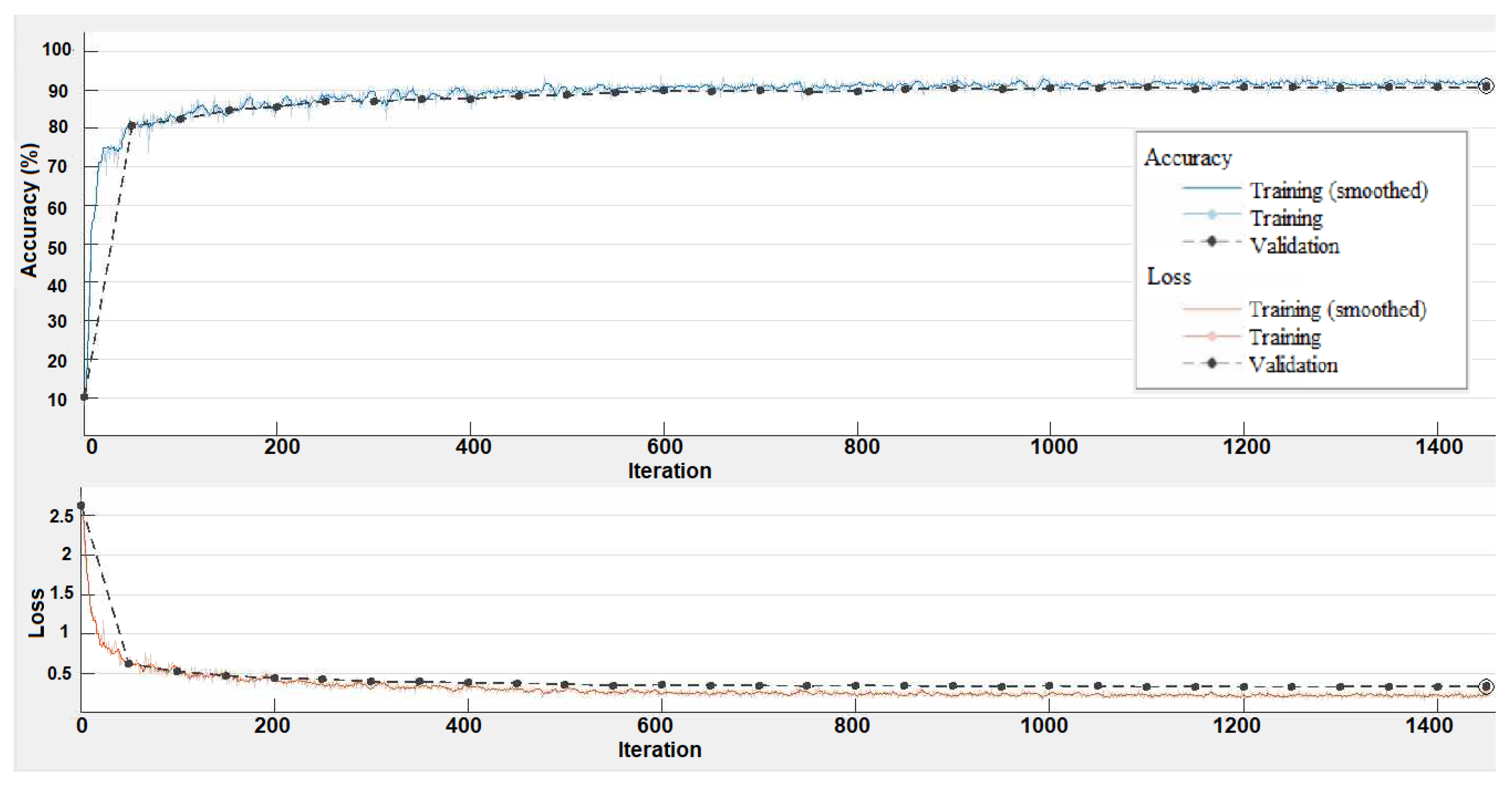
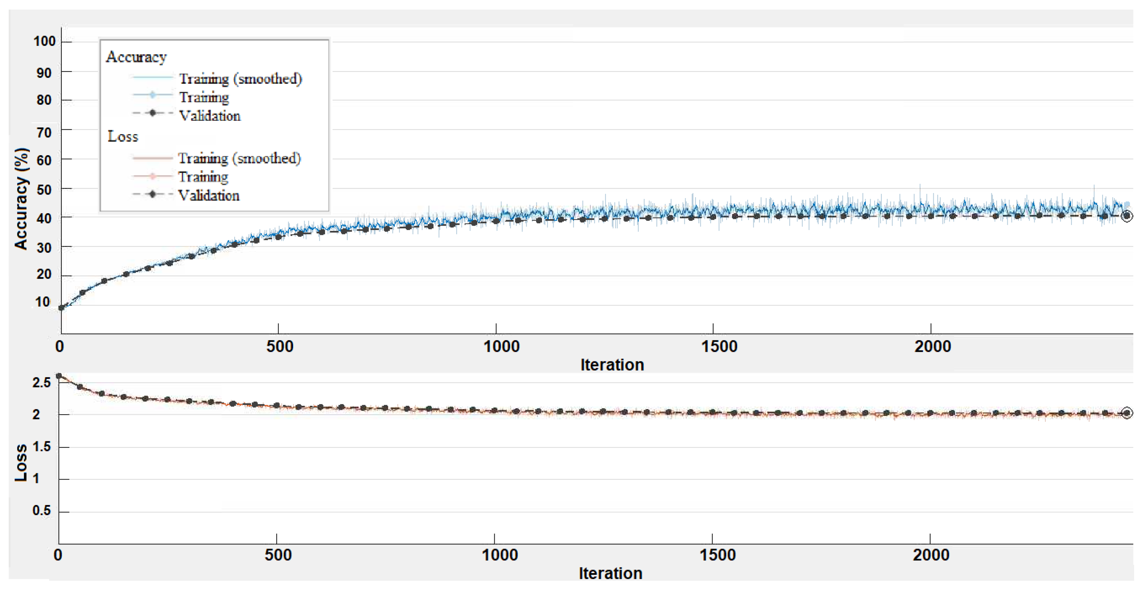
Figure 5 shows the training progress of the DeepLabV3+ network to prepare it for the LBLS model. The graph reveals the classification accuracy achieved on each mini-batch, reaching a value of 90%. This high accuracy suggests that the network is performing well and making accurate predictions during the training process. Furthermore, the training loss graph indicates the loss on each mini-batch, with a value of 0.4. This low training loss demonstrates that the model is effectively reducing the discrepancy between its predicted outputs and the true labels. By minimizing the loss function, the model is optimizing its parameters to improve its predictive capabilities.

Figure 6 illustrates the training progress of the FCN network to prepare it to be used in the LBLS model. The graph displays the classification accuracy achieved on each mini-batch, reaching a value of 70%. This accuracy value suggests that the network is making reasonably accurate predictions during the training process. The training loss graph provides information about the loss on each mini-batch, with a value of 0.1. This indicates that the model is effectively reducing the discrepancy between its predicted outputs and the true labels, as a lower training loss corresponds to a better alignment between predictions and ground truth.

Moreover, Figure 7 depicts the training progress of the SegNet network to prepare it to be used in the LBLS model. The graph shows classification accuracy on each mini-batch, in which it reaches 40%. The training loss graph provides information about the loss on each mini-batch, in which it reaches a value of 2.

Furthermore, Figure 7 illustrates the training progress of the SegNet network to prepare it to be used in the LBLS model. The graph represents the classification accuracy achieved on each mini-batch, reaching a value of 40%. The training loss graph provides information about the loss on each mini-batch, with a value of 2.

The lower accuracy and higher training loss of the SegNet model compared to DeepLabV3+ and FCN are primarily due to the inherent architecture of SegNet, which, while effective for many segmentation tasks, may struggle with complex sky region segmentation due to its relatively simpler encoder-decoder structure. SegNet does not incorporate advanced techniques like atrous convolutions or multi-scale feature aggregation, which are present in DeepLabV3+ and FCN. These limitations can lead to reduced performance, especially in scenarios with complex backgrounds, varying lighting conditions, and occlusions, as observed in the CamVid dataset.

Despite the lower baseline performance of SegNet, the integration of the LBLS model significantly improved its segmentation results, as will be seen in the next section. The low accuracy and high loss during SegNet training can be attributed to the fact that the CamVid dataset contains a wide range of outdoor scenes with significant variations in lighting, shadows, and occlusions, which can challenge simpler models like SegNet. In addition, SegNet’s architecture lacks the multi-scale feature extraction capabilities of DeepLabV3+ and FCN, making it less effective at capturing fine details and contextual information. Moreover, the training process for SegNet may require more extensive hyperparameter tuning or data augmentation to achieve better convergence. However, even with these limitations, the addition of LBLS provided a noticeable improvement in segmentation quality.

3. Results and Discussion

3.1. Visual Evaluation

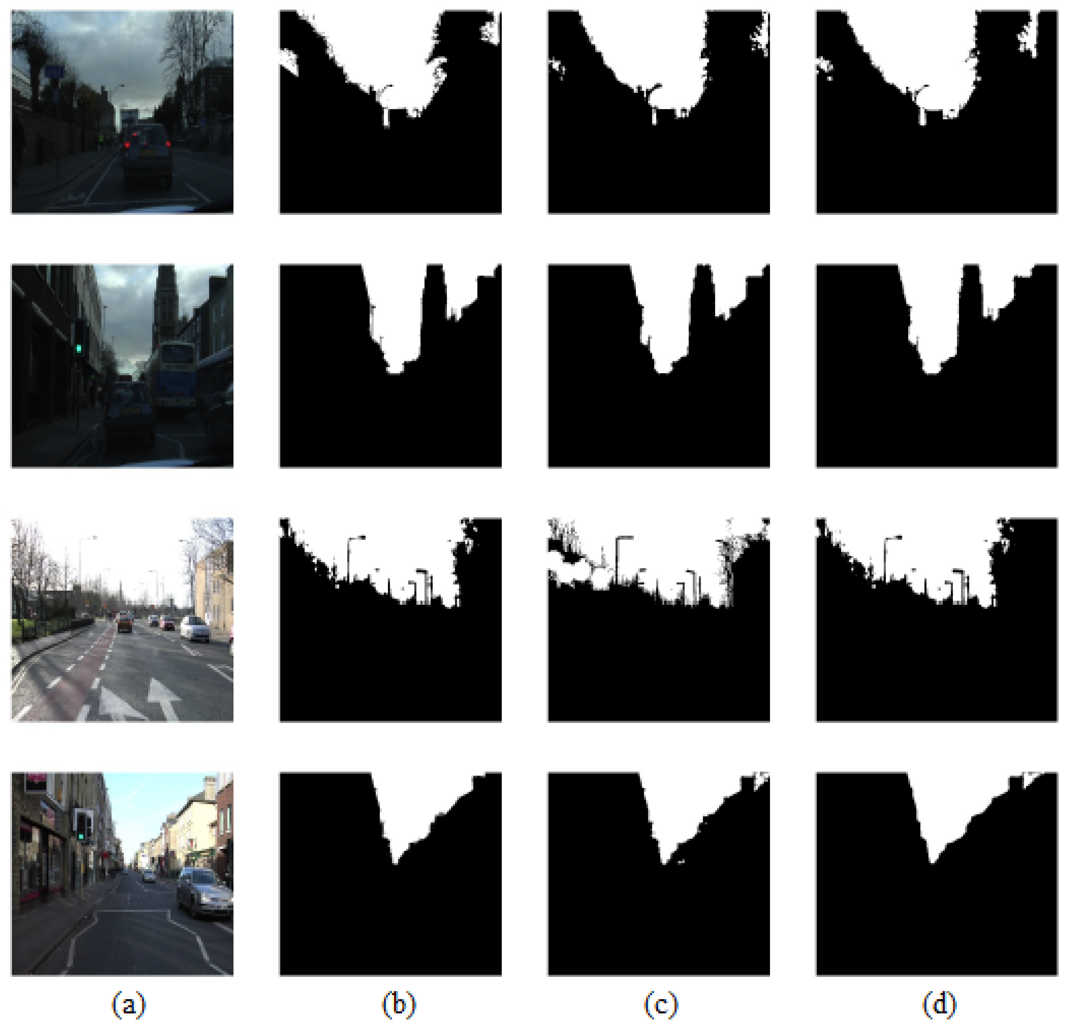
In this section, we conduct a visual evaluation of the results obtained from our proposed algorithm. Figure 8 presents the visual comparison of the outputs when applying DeepLabV3+ with and without LBLS (Lattice Boltzmann Level Set) on randomly selected testing images. The purpose was to assess the performance of our algorithm by comparing the results to the ground truth imagery.

Upon examining Figure 8, it is evident that the results achieved using DeepLabV3+ with LBLS exhibit a closer resemblance to the ground truth imagery. The visual comparison highlights the effectiveness of incorporating LBLS into the DeepLabV3+ algorithm, as it leads to improved segmentation results.

By utilizing DeepLabV3+ with LBLS, the algorithm demonstrates a higher level of accuracy in delineating object boundaries and preserving fine details. The segmentation outputs show smoother and more coherent contours, resulting in a visually appealing and closer representation of the true objects in the images.

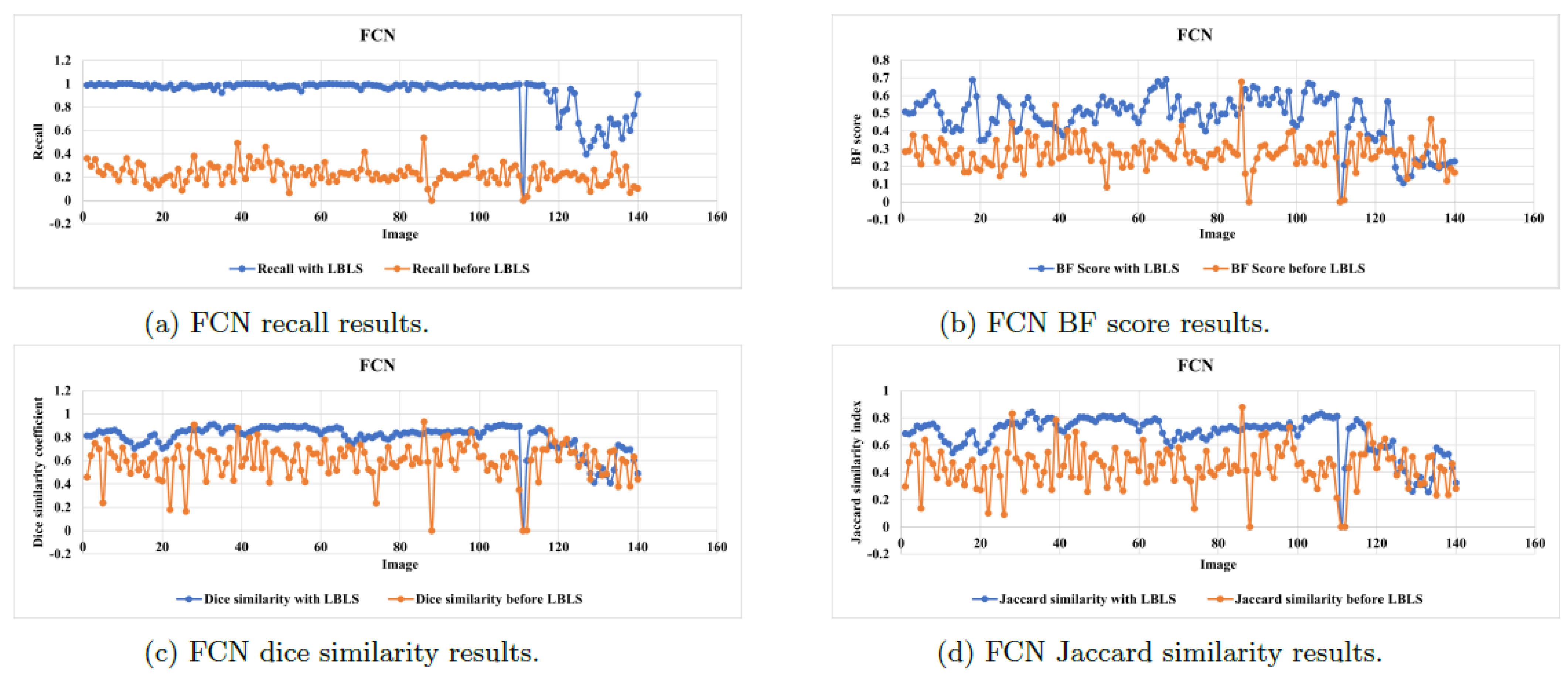
This visual evaluation provides qualitative evidence supporting the superiority of DeepLabV3+ with LBLS over the version without LBLS. The enhanced performance of the algorithm is evident in terms of its ability to produce segmentation results that are visually closer to the ground truth imagery. Moreover, we further evaluated the performance of our proposed algorithm by applying FCN (Fully Convolutional Network) with and without LBLS on randomly selected testing images. The results of this evaluation are presented in Figure 9, which showcases the comparison between the outputs obtained using FCN with and without LBLS, as well as their proximity to the ground truth imagery.

Upon analyzing Figure 9, it becomes apparent that the results achieved with FCN utilizing LBLS exhibit a higher degree of similarity to the ground truth imagery. The visual comparison clearly illustrates that incorporating LBLS into the FCN algorithm leads to improved segmentation results.

Incorporating LBLS into FCN shows better object completeness and better preservation of fine details and textures. The segmentation outputs showcase smoother contour delineation and a more cohesive representation of the true objects in the images.

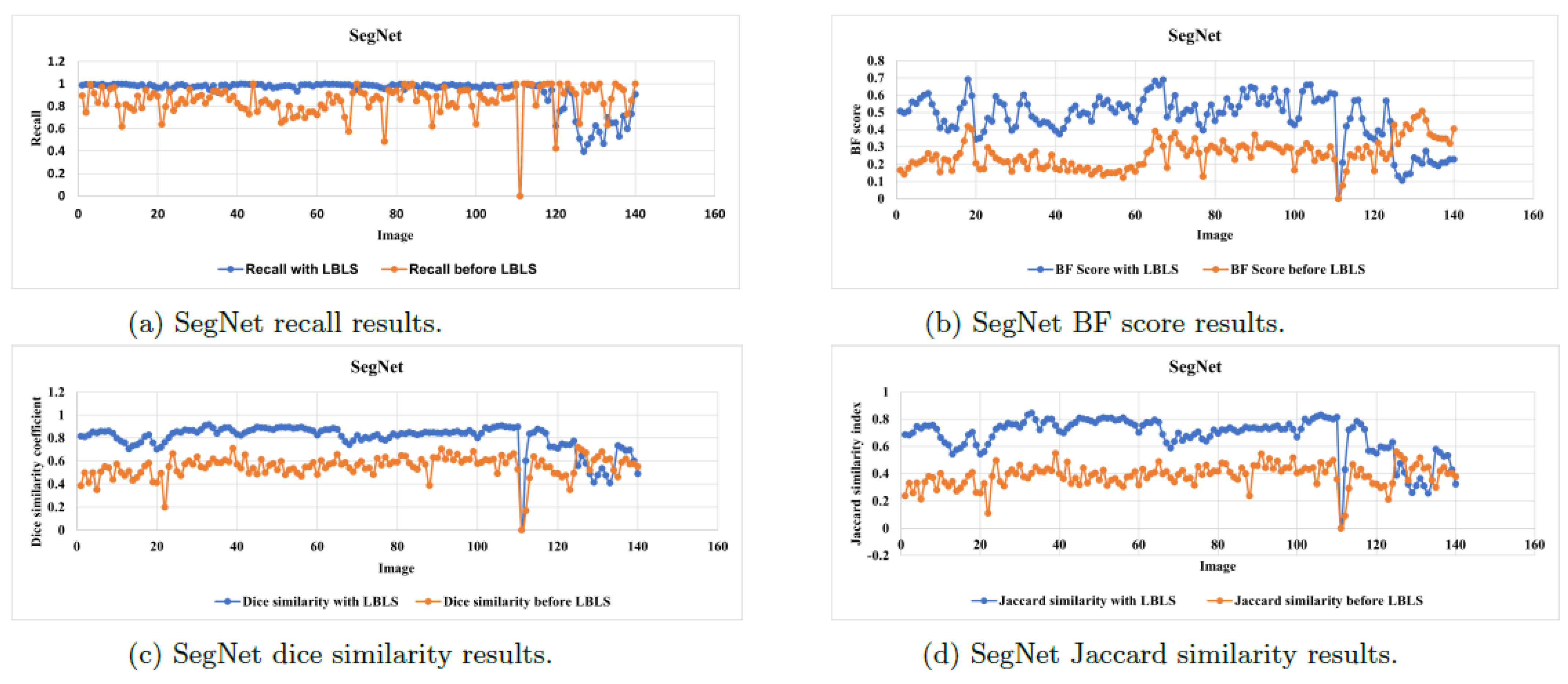
This visual evaluation provides compelling evidence supporting the effectiveness of FCN with LBLS over the version without LBLS. The inclusion of LBLS enhances the algorithm’s ability to produce segmentation results that closely resemble the ground truth imagery. In addition to the evaluations conducted on DeepLabV3+ and FCN, we also assessed the performance of SegNet, both with and without LBLS, on randomly selected testing images. Figure 10 provides a visual representation of the obtained results, highlighting the comparison between the outputs achieved using SegNet with and without LBLS, as well as their proximity to the ground truth imagery.

Upon careful examination of Figure 10, it is evident that the results obtained with SegNet incorporating LBLS exhibit a closer resemblance to the ground truth imagery. The visual comparison clearly demonstrates the effectiveness of integrating LBLS into the SegNet algorithm, as it leads to improved segmentation results.

By utilizing SegNet with LBLS, the algorithm excels in accurately delineating object boundaries, ensuring object completeness, and preserving fine details and textures. The segmentation outputs showcase smoother contours and a higher level of visual coherence, resulting in a more accurate representation of the true objects in the images.

This visual evaluation provides strong evidence supporting the superiority of SegNet with LBLS over the version without LBLS. The incorporation of LBLS significantly enhances the algorithm’s segmentation performance, leading to results that closely align with the ground truth imagery.

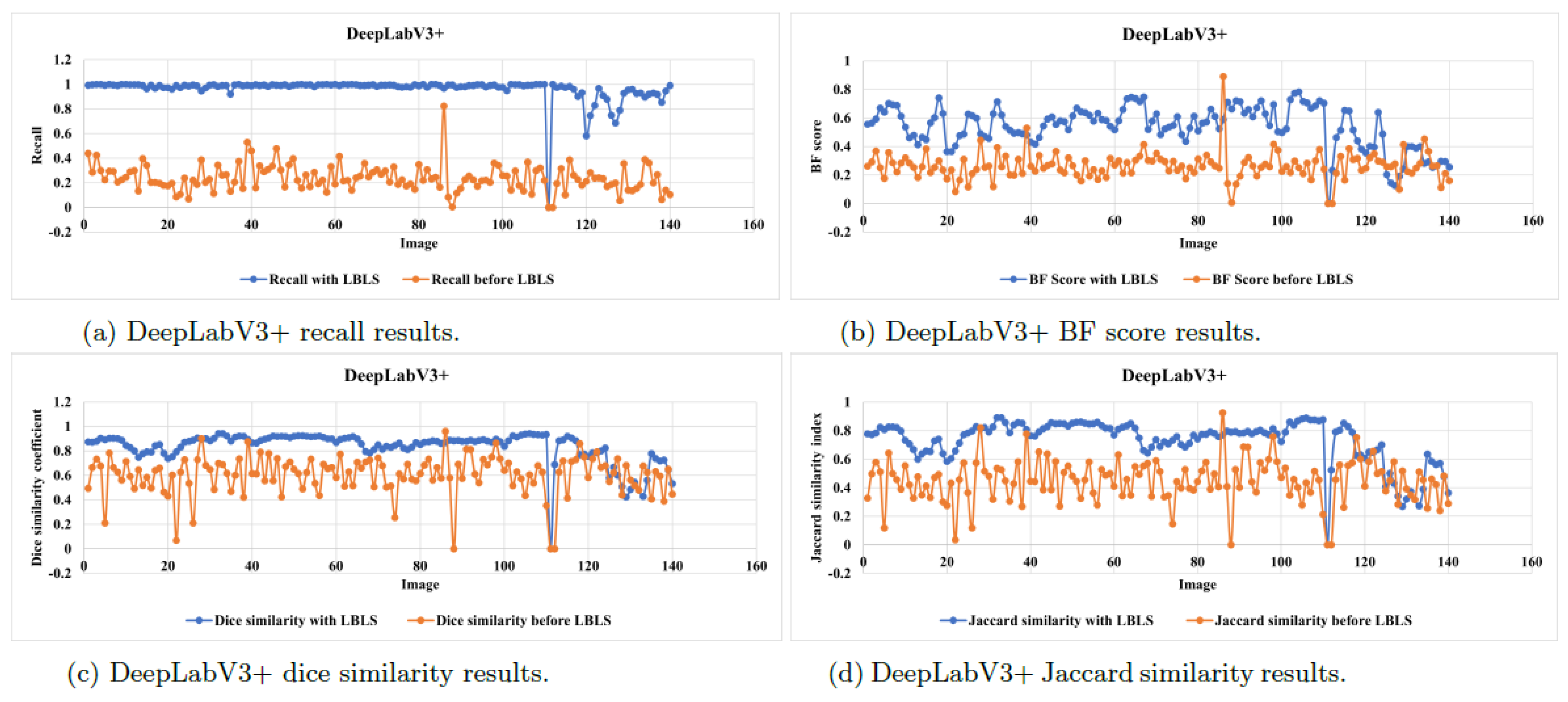
3.2. Quantitative Evaluation

Figure 11 illustrates the evaluation metrics applied with the DeepLabV3+ NN before and after applying the LBLS segmentation. Figure 11a shows the recall value of the sky region segmentation before and after applying lattice Boltzmann level-set (LBLS) segmentation. The output of the deep learning semantic segmentation using the DeepLabV3+ neural network is compared with the ground truth before and after applying the LBLS segmentation. It is observed that the recall value is significantly improved when utilizing LBLS segmentation.

Additionally, Figure 11b illustrates the $BFscore$ for testing images of the sky region segmentation before and after the application of LBLS segmentation. The $BFscore$ is a widely used metric for assessing the accuracy of boundary detection or segmentation algorithms. It quantifies the similarity between the detected boundaries and the ground truth boundaries.

Figure 11 also demonstrates higher values of the $BFscore$ after the LBLS segmentation is applied. This indicates that the boundaries of the sky region are more accurately detected and aligned with the ground truth boundaries. Consequently, the LBLS segmentation technique has effectively improved the boundary detection in the sky region, resulting in enhanced segmentation quality. Furthermore, Figure 11c illustrates the Dice similarity coefficient for testing images of the sky region segmentation before and after the application of LBLS segmentation.

The Dice similarity coefficient is a widely used metric for evaluating the similarity or overlap between two sets, such as the predicted and ground truth segmentation masks in image segmentation tasks. It is calculated by taking twice the intersection of the predicted and ground truth regions and dividing it by the sum of the sizes of both regions. The coefficient ranges from 0 to 1, where 1 indicates a perfect overlap or similarity between the predicted and ground truth regions, and 0 indicates no overlap.

The graph demonstrates an increase in the Dice similarity coefficient after the application of LBLS segmentation. This indicates an improvement in the accuracy and alignment of the segmented sky regions with the ground truth regions. The boundaries and overall segmentation of the sky region are more closely aligned with the true regions. A higher Dice coefficient signifies a greater degree of overlap between the predicted and ground truth regions, which suggests enhanced segmentation accuracy.

Based on the results mentioned above, the LBLS segmentation technique can effectively improve the segmentation quality of the sky region, leading to a higher level of similarity between the segmented regions and the ground truth. The increase in the Dice similarity coefficient demonstrates the success of LBLS in accurately aligning the segmented sky regions with the true regions, resulting in improved segmentation accuracy. Moreover, Figure 11d illustrates the Jaccard similarity index of testing images of the sky region segmentation before and after applying LBLS segmentation.

The Jaccard similarity index, also known as the Jaccard coefficient or Intersection over Union (IoU), is a metric commonly used to evaluate the similarity or overlap between two sets, such as the predicted and ground truth segmentation masks in image segmentation tasks. The Jaccard similarity index is calculated as the ratio of the intersection of the predicted and ground truth regions to the union of the predicted and ground truth regions. It ranges from 0 to 1, where a value of 1 indicates a perfect overlap or similarity between the predicted and ground truth regions, and a value of 0 indicates no overlap.

Figure 11 shows that the Jaccard similarity index increases after applying LBLS segmentation; it indicates an improvement in the accuracy and alignment of the segmented sky regions with the ground truth regions. This means that the boundaries and overall segmentation of the sky region are more closely aligned with the true regions. It also implies that the LBLS segmentation technique has successfully enhanced the segmentation quality of the sky region, resulting in a higher level of similarity with the ground truth. Similarly, Figure 12 and Figure 13 illustrate the segmentation metrics of recall, $BFscore$, dice similarity coefficient, and Jaccard similarity index values for the testing images of the sky region segmentation before and after applying LBLS segmentation for both FCN and SegNet, respectively. The figures provide an indication of the improvement in segmentation results after the application of LBLS. Therefore, our proposed deep LBLS methodology enhances robustness and improves the accuracy of the segmentation results. Thus, the proposed deep LBLS technique improves boundary detection of the sky region through its inherent characteristics and capabilities. This is because deep LBLS segmentation leverages spatial information to capture the boundaries accurately. The level-set framework allows for the representation of complex boundary shapes and topological changes over time. By utilizing this representation, LBLS can effectively model the intricate boundaries often present in the sky region. Additionally, the level-set equation in LBLS segmentation involves a cost function that guides the evolution of the level-set function. This cost function typically includes terms related to data fidelity and regularization. The data fidelity term ensures that the evolving boundary aligns with the observed image data, while the regularization term promotes smoothness and regularity. By optimizing this cost function, LBLS aims to minimize the discrepancy between the detected boundaries and the ground truth boundaries. Moreover, the use of atrous convolution and feature extraction techniques helps to capture relevant information for boundary detection. Atrous convolution allows for larger receptive fields, enabling the model to capture contextual information and improve boundary localization. Feature extraction techniques help extract meaningful features from the input images, which can aid in accurately detecting boundaries in the sky region. Finally, the iterative nature of LBLS segmentation allows for ongoing refinement of the boundary detection process. The level-set function evolves over multiple iterations, gradually aligning with the ground truth boundaries. This iterative refinement helps improve the accuracy and alignment of the detected boundaries with the true boundaries in the sky region.

By combining these elements, the LBLS segmentation technique enhances boundary detection in the sky region. It leverages spatial information, optimizes the cost function, incorporates advanced techniques like atrous convolution and feature extraction, and iteratively refines the detected boundaries. This comprehensive approach yields improved segmentation quality by accurately detecting and aligning boundaries with the ground truth, resulting in enhanced boundary detection in the sky region.

3.3. Performance Comparison Between the Three CNNs with and Without LBLS

From

Table 2. Performance comparison between the three used NNs.

Method	Mean Recall	Mean BF Score	Mean Dice Similarity	Mean Jaccard Index
DeepLabV3+ (without LBLS)	0.82464294	0.857826	0.938691	0.892261
DeepLabV3+ (with LBLS)	0.969233	0.874401	0.940048	0.893606
FCN (without LBLS)	0.649962	0.729197	0.906361	0.838899
FCN (with LBLS)	0.699643	0.757435	0.909279	0.841364
SegNet (without LBLS)	0.755992	0.825062	0.926336	0.871246
SegNet (with LBLS)	0.886145	0.873888	0.928046	0.873867

, it can be observed that in all three cases, our deep Lattice Boltzmann Level Set (deep LBLS) approach demonstrates better performance. For example: (1) DeepLabV3+ shows improvements of 14.45% in mean recall, 1.65% in mean $BFscore$, 0.136% in mean dice similarity coefficient, and 0.134% in mean Jaccard similarity index. (2) FCN exhibits improvements of 4.96% in mean recall, 2.82% in mean $BFscore$, 0.29% in mean dice similarity coefficient, and 0.24% in mean Jaccard similarity index. (3) SegNet displays improvements of 13.01% in mean recall, 4.88% in mean $BFscore$, 0.17% in mean dice similarity coefficient, and 0.26% in mean Jaccard similarity index. When comparing the three CNNs, DeepLabV3+ yields the best results for our object of interest segmentation.

The superiority of DeepLabV3+ over FCN and SegNet for the sky region segmentation can be attributed to the fact that DeepLabV3+ utilizes an advanced architecture specifically designed for semantic segmentation tasks. It incorporates atrous spatial pyramid pooling (ASPP), enabling multi-scale feature aggregation and effectively capturing contextual information. This architecture allows DeepLabV3+ to capture fine-grained details and maintain spatial resolution, resulting in better object segmentation. Moreover, because DeepLabV3+ employs dilated convolutions, also known as atrous convolutions, it expands the receptive field of the network without downsampling the feature maps. By incorporating dilated convolutions, DeepLabV3+ can capture information from a wider context while preserving fine details. This is particularly beneficial for objects with intricate structures or detailed textures.

3.4. Computation Speed

The time consumption was measured before and after implementing the lattice Boltzmann approach. Specifically, we compare the processing time of the deep lattice Boltzmann level-set (LBLS) with the three CNN models mentioned above to assess computation speed.

Table 3. Average computational time of sky region segmentation.

Method	Time (s)
DeepLabV3+ LS	4.7776
DeepLabV3+ LBLS	1.1536
FCN LS	1.2795
FCN LBLS	1.1817
SegNet LS	1.7932
SegNet LBLS	1.1487

presents the average time consumption comparison for all methods on the test set images. These results demonstrate that utilizing the LBLS significantly reduces computational time consumption.

It is important to notice that our deep Lattice Boltzmann Level set (deep LBLS) approach can reduce computational time due to several factors. One factor is that the lattice Boltzmann method (LBM), which is utilized in the LBLS approach, is known for its computational efficiency. LBM employs a simplified lattice-based grid structure and efficient numerical schemes to simulate fluid flow or interface evolution. This efficiency translates into reduced computational time compared to other methods. Moreover, our deep LBLS focuses on local computations within each lattice cell, which reduces the overall computational complexity. Instead of solving complex equations for the entire domain, deep LBLS performs calculations locally, simplifying the processing required and leading to faster execution. These factors enable deep LBLS to streamline computations and enhance computational efficiency compared to other methods, leading to faster processing times.

4. Conclusions

Sky region segmentation plays a significant role in various areas of image processing, contributing to scene understanding, image enhancement, retrieval systems, AR/VR applications, environmental monitoring, and video production. In this paper, we present a fast and robust approach for sky region extraction called deep learning lattice Boltzmann level-set segmentation (deep LBLS). Our method combines deep learning, the level-set method (LS), and the lattice Boltzmann method (LBM) to achieve accurate and efficient sky region segmentation while preserving fine details crucial for object identification and scene understanding. We introduce a newly formulated level-set function based on deep learning, enabling precise segmentation. The learning criteria of the level-set are achieved through deep neural networks. To accelerate the curve evolution process, we utilize LBM, ensuring faster convergence of the level-set function. Experimental results demonstrate that our proposed deep LBLS approach outperforms state-of-the-art learning-based methods in segmenting the sky region in natural visible images, achieving both superior accuracy and speed.

Moving forward, our future research will focus on exploring the application of the deep LBLS approach in satellite imagery for cloud detection and atmospheric analysis. Moreover, we will investigate the adaptability of the proposed method for real-time sky segmentation in drone imagery and aerial surveillance. Beyond sky region segmentation, the proposed deep LBLS approach has the potential to be adapted to other image segmentation tasks, such as medical imaging, where precise boundary detection and rapid convergence are critical. For instance, the method could be applied to segment tumors in medical scans or to delineate anatomical structures in MRI and CT images. Additionally, the approach could be extended to other domains, such as autonomous driving, where accurate segmentation of road scenes, including sky, road, and obstacles, is essential for navigation and safety. The versatility of the deep LBLS framework makes it a promising candidate for a wide range of segmentation challenges across different fields.