Article

Fourth-Order Numerical Derivation as Being an Inverse Force Problem of Beam Equations

1
Center of Excellence for Ocean Engineering, National Taiwan Ocean University, Keelung 202301, Taiwan
2
Department of Mechanical Engineering, National United University, Miaoli 360302, Taiwan
*
Author to whom correspondence should be addressed.
Eng 2025, 6(11), 324; https://doi.org/10.3390/eng6110324
Submission received: 22 September 2025 / Revised: 4 November 2025 / Accepted: 6 November 2025 / Published: 11 November 2025

Abstract

Besides the closed-form expansion coefficients of a weak-form numerical differentiator (WFND), we introduce a cubic boundary shape function with the aid of two parameters for reducing the boundary errors of fourth-order numerical derivatives to zero. So that the accuracy of numerical derivatives obtained by the new WFND can be improved significantly. The fourth-order numerical derivation can be modeled as a linear beam equation subjecting to specified boundary conditions and displacements to recover an unknown forcing term. By means of boundary shape functions, two numerical collocation methods automatically satisfying the boundary conditions are developed. For a simply supported linear Euler–Bernoulli beam with an elastic foundation, the unknown spatially–temporally dependent force is retrieved. The displacement at a final time and strain on the right-boundary of the beam are over-specified to recover the external force using the method of superposition of boundary shape functions (MSBSF). When the displacement is determined to satisfy the prescribed right-boundary strain, we can recover an unknown spatially–temporally dependent force by inserting the displacement into the linear beam equation. An embedded method (EM) is developed to transform the linear beam model into a vibrating linear beam equation, and then we can develop a robust technique to compute the fourth-order derivative of noisy data by using the EM and MSBSF. The four proposed methods for evaluating the fourth-order derivatives of noisy data are efficient and accurate.

1. Introduction

The n-th order numerical differentiation of a noisy signal in time is to recover a function f ( t ) on the right-hand side of an n-th order ordinary differential equation (ODE): x ( n ) ( t ) = f ( t ) . It is a highly ill-posed inverse problem because a small unavoidable perturbation of x ( t ) may result in a large error of the derivative [1]. The numerical differentiation is widely used in many inverse problems to retrieve unknown physical functions of variables, and has many engineering applications [2,3,4,5].
The differentiation of noisy data is an old and challenging problem, but it is a seriously ill-posed problem [1]. The fourth-order derivative of a function g ( t ) leads to differential algebraic equations:
x ˙ 0 ( t ) = x 1 ( t ) , x ˙ 1 ( t ) = x 2 ( t ) , x ˙ 2 ( t ) = x 3 ( t ) , x ˙ 3 ( t ) = x 4 ( t ) ,
x 0 ( t ) g ( t ) = 0 .
When Equation (2) is an algebraic equation, Equation (1) consists of a set of first-order ODEs with x i , i = 1 , , 4 the ith order derivative of g ( t ) . These differential operators are unbounded, such that one usually cannot obtain the correct solutions of x i ( t ) . Moreover, the above differential algebraic equations have index-five, which is very difficult to solve using a numerical method [6].
In the literature, most results are concerned with the first-order and second-order differentiation methods, which include the Euler method [7,8], the numerical differentiator [9,10,11,12], the sliding mode differentiator [13,14,15,16], the finite difference method [17], the polynomial interpolation method [18,19], the regularization method [20,21,22], the kernel-based numerical differentiation methods [23,24], and the fast Fourier transform method [25]. There are rare methods which can compute the fourth-order derivative accurately. Liu and Dong [26] proposed a closed-form fourth-order numerical differentiator for differentiating the noisy data four times by using the weak-form numerical differentiator (WFND). Duan and Wang [27] developed a regularization method for computing the fourth-order derivative and applied it in fluid–structure interactions.
This paper may shed a light on the solutions of higher-order numerical derivatives of noisy data using simple methods. One of the new techniques is that we model the fourth-order derivative problem as being an inverse force problem of a linear beam equation:
x ( 4 ) ( t ) = f ( t ) ,
which is subject to boundary conditions and is solvable in a weak sense. When the data of x ( t ) = g ( t ) are measured with noisy errors, the unknown force f ( t ) is recovered. It is an inverse force problem of the beam Equation (3), which provides the measured data of x ( t ) = g ( t ) and subjects the beam to prescribed boundary conditions as supplementary data. The forced vibrations of beams spur many applications in building structures, mechanical cutting tools, structural engineering, aerospace vehicles, and aircraft engineering [28,29,30]. Sometimes, the exerted forces acting on the beam are unknown and need to be identified [31,32,33], which corresponds to an inverse force problem of the beam equations.

2. Mathematical Preliminaries of WFND

By means of a weak sense solution of Equation (3) with sinusoidal functions as test functions and basis functions, the following results were proven in [26].
Theorem 1 
(Liu and Dong [26]). Given x ( t ) = g ( t ) , 0 t t f , z ( t ) = x ¨ ( t ) satisfies the following integral equation:
0 t f z ( t ) sin j π t t f d t = j π t f [ g ( 0 ) g ( t f ) cos j π ] j 2 π 2 t f 2 0 t f g ( t ) sin j π t t f d t ,
where j N is a free index.
Theorem 2 
(Liu and Dong [26]). Given x ( t ) = g ( t ) , 0 t t f , w ( t ) = x ( 4 ) ( t ) is governed by the following integral equation:
0 t f w ( t ) sin j π t t f d t = j π t f [ z ( 0 ) z ( t f ) cos j π ] + j 3 π 3 t f 3 [ g ( t f ) cos j π g ( 0 ) ] + j 4 π 4 t f 4 0 t f g ( t ) sin j π t t f d t ,
where j N is a free index, and z ( 0 ) and z ( t f ) are derived from Theorem 1.
Proof. 
Let
x ( 4 ) ( t ) = w ( t ) , 0 < t t f .
Applying the test function v j ( t ) = sin ( j π t / t f ) to Equation (6) and integrating it from t = 0 to t = t f , we can obtain a weak-form integral equation:
0 t f w ( t ) v j ( t ) d t = 0 t f x ( 4 ) ( t ) v j ( t ) d t .
Integration by parts of the right-hand side twice yields
0 t f x ( 4 ) ( t ) v j ( t ) d t = j π t f 0 t f x ( t ) cos j π t t f d t = j π t f [ z ( 0 ) z ( t f ) cos j π ] j 2 π 2 t f 2 0 t f z ( t ) sin j π t t f d t ,
due to v j ( 0 ) = v j ( t f ) = 0 for the test functions v j ( t ) . Using w ( t ) = x ( 4 ) ( t ) and inserting Equation (4) for the last integral term into Equation (8), we can derive Equation (5). □
Then, Liu and Dong [26], by inserting
z ( t ) = z ( 0 ) + t t f [ z ( t f ) z ( 0 ) ] + k = 1 m a k sin k π t t f ,
w ( t ) = w ( 0 ) + t t f [ w ( t f ) w ( 0 ) ] + k = 1 m b k sin k π t t f
into the weak-form integral Equations (4) and (5), and setting a m + 1 : = z ( 0 ) , a m + 2 : = z ( t f ) , b m + 1 : = w ( 0 ) and b m + 2 : = w ( t f ) , obtained the following closed-form solution of the coefficients a k , k = 1 , , m + 2 for z ( t ) :
a 1 a m a m + 1 a m + 2 = 2 t f I m 2 t f B C 1 0 C 1 e 1 e m e m + 1 e m + 2 , B j 1 = 0 t f 1 t t f sin j π t t f d t = t f j π , j = 1 , , m ,
B j 2 = 0 t f t t f sin j π t t f d t = t f cos j π j π , j = 1 , , m , C 11 = 0 t f 1 t t f sin ( m + 1 ) π t t f d t = t f ( m + 1 ) π , C 12 = 0 t f t t f sin ( m + 1 ) π t t f d t = t f cos ( m + 1 ) π ( m + 1 ) π , C 21 = 0 t f 1 t t f sin ( m + 2 ) π t t f d t = t f ( m + 2 ) π ,
C 22 = 0 t f t t f sin ( m + 2 ) π t t f d t = t f cos ( m + 2 ) π ( m + 2 ) π ,
e j : = j π t f [ g ( 0 ) g ( t f ) cos j π ] j 2 π 2 t f 2 0 t f g ( t ) sin j π t t f d t , j = 1 , , m + 2 .
In the above, B is an m × 2 matrix, which consists of first column vector { B j 1 , j = 1 , , m } and second column vector { B j 2 , j = 1 , , m } . C is a 2 × 2 matrix, which consists of four elements C 11 , C 12 , C 21 , and C 22 . Hence, B C 1 is an m × 2 matrix. Because B is normalized by C 1 , the term B C 1 in Equation (11) is dimensionless.
Similarly, Liu and Dong [26] obtained the following closed-form solution of the coefficients b k , k = 1 , , m + 2 for w ( t ) :
b 1 b m b m + 1 b m + 2 = 2 t f I m 2 t f B C 1 0 C 1 q 1 q m q m + 1 q m + 2 ,
where
q j : = j π t f [ a m + 1 a m + 2 cos j π ] + j 3 π 3 t f 3 [ g ( t f ) cos j π g ( 0 ) ] + j 4 π 4 t f 4 0 t f g ( t ) sin j π t t f d t , j = 1 , , m + 2 .
Here, w ( t ) is not independent of z ( t ) , which is related to z ( t ) through the coefficients a m + 1 = z ( 0 ) and a m + 2 = z ( t f ) .
It follows from Equation (13) that
C 11 C 12 C 21 C 22 = t f 2 [ cos ( m + 1 ) π cos ( m + 2 ) π ] ( m + 1 ) ( m + 2 ) π 2 ,
and C 1 is available as follows:
C 1 = ( m + 1 ) ( m + 2 ) π 2 t f 2 [ cos ( m + 1 ) π cos ( m + 2 ) π ] C 22 C 12 C 21 C 11 .
Therefore, the coefficients a k in Equation (11) and b k in Equation (15) can be determined exactly in closed form. When m is a large integer, the determinant of C is small, such that its inverse C 1 has a large value.
The drawback of Equation (15) is that a m + 1 = z ( 0 ) and a m + 2 = z ( t f ) appear in q j , as shown by Equation (16), in which, due to C 1 in Equations (15) and (18), the boundary errors of z ( 0 ) and z ( t f ) would be amplified to larger boundary errors of w ( t ) as follows:
w ( 0 ) w ( t f ) = C 11 C 12 C 21 C 22 1 q m + 1 q m + 2 .
Notice that when we take the second-order derivative of Equation (9) to compute the fourth-order derivative w ( t ) , it leads to w ( 0 ) = 0 and w ( t f ) = 0 , which may not hold generally. To overcome this drawback, we employ Equation (10) to compute the fourth-order derivative w ( t ) , which is better than taking the second-order derivative of Equation (9) to compute the fourth-order derivative w ( t ) .

3. Reducing Boundary Errors of Fourth-Order Derivative

In practice, when one applies the above method to test the examples for computing the fourth-order derivative, there appear large boundary errors as shown in Figures 8b and 9d of [26]. To remedy this drawback of the original WFND, we can consider a new boundary shape function α ( t ) to reduce the boundary errors by taking
z ( t ) = 1 α ( t ) c m + 1 + α ( t ) c m + 2 + k = 1 m c k sin k π t t f x ¨ ( t ) ,
where c m + 1 : = z ( 0 ) and c m + 2 : = z ( t f ) , and c k , k = 1 , , m + 2 are unknown coefficients to be given below. The boundary shape function α ( t ) satisfies α ( 0 ) = 0 and α ( t f ) = 1 . To satisfy the above two boundary conditions, the boundary shape function α ( t ) must be a time-varying function.
Rather than α = t / t f used in Equation (9), we consider the following cubic boundary shape function:
α ( t ) = ( 1 γ β ) t t f + γ t t f 2 + β t t f 3 ,
where γ and β are parameters used to reduce the boundary errors of the fourth-order derivative.
The idea for the introduction of α ( t ) in Equation (21) is that we have two extra parameters γ and β , to render w ( 0 ) = x ( 4 ) ( 0 ) and w ( t f ) = x ( 4 ) ( t f ) such that the two parameters γ and β can be determined to reduce the boundary errors of the fourth-order derivative.
Inserting t = 0 into Equation (21) yields α ( 0 ) = 0 . Inserting t = t f into Equation (21) yields
α ( t f ) = 1 γ β + γ + β = 1 ,
which satisfies α ( t f ) = 1 automatically.
The unknown coefficients c k , k = 1 , , m + 2 are determined by
c 1 c m c m + 1 c m + 2 = 2 t f I m 2 t f B C 1 0 C 1 e 1 e m e m + 1 e m + 2 ,
where e j are still defined by Equation (14), but with the new coefficient matrix given by
B j 1 = 0 t f 1 α ( t ) sin j π t t f d t , B j 2 = 0 t f α ( t ) sin j π t t f d t , j = 1 , , m , C 11 = 0 t f 1 α ( t ) sin ( m + 1 ) π t t f d t , C 12 = 0 t f α ( t ) sin ( m + 1 ) π t t f d t ,
C 21 = 0 t f 1 α ( t ) sin ( m + 2 ) π t t f d t , C 22 = 0 t f α ( t ) sin ( m + 2 ) π t t f d t .
If we take α ( t ) = t / t f , Equations (23) and (24) recover to Equations (12) and (13).
Due to the dependence of the coefficients in Equations (23) and (24) on α ( t ) , which is a cubic function of t, the closed-form formulas such as those in Equations (12) and (13) are no longer available. Instead, we apply the Gaussian quadrature to compute the coefficients in Equations (23) and (24).
Furthermore, we can compute the higher-order derivatives of noisy signals, which are available by sequentially taking the time derivatives of Equation (20) to the order we need:
y ( t ) : = z ˙ ( t ) = ( c m + 2 c m + 1 ) α ˙ ( t ) + k = 1 m k π c k t f cos k π t t f x ( t ) ,
w ( t ) : = z ¨ ( t ) = ( c m + 2 c m + 1 ) α ¨ ( t ) k = 1 m k 2 π 2 c k t f 2 sin k π t t f x ( 4 ) ( t ) ,
where
α ˙ ( t ) = 1 γ β t f + 2 γ t t f 2 + 3 β t 2 t f 3 , α ¨ ( t ) = 2 γ t f 2 + 6 β t t f 3
are derived from Equation (21).
Theorem 3 .
We assume that z ( 0 ) z ( t f ) . There exist two parameters:
γ = t f 2 x ( 4 ) ( 0 ) 2 ( c m + 2 c m + 1 ) , β = t f 2 [ x ( 4 ) ( t f ) x ( 4 ) ( 0 ) 6 ( c m + 2 c m + 1 ) ,
such that the fourth-order numerical derivative provided by Equation (26) can exactly match the end values of the true fourth-order derivative x ( 4 ) ( t ) with w ( 0 ) = x ( 4 ) ( 0 ) and w ( t f ) = x ( 4 ) ( t f ) .
Proof. 
Under the assumption of z ( 0 ) z ( t f ) , we have
c m + 2 c m + 1 0 .
From Equations (26) and (27), it follows that
x ( 4 ) ( 0 ) = ( c m + 2 c m + 1 ) 2 γ t f 2 ,
x ( 4 ) ( t f ) = ( c m + 2 c m + 1 ) 2 γ t f 2 + 6 β t f 2 ,
where
k = 1 m k 2 π 2 c k t f 2 sin 0 = 0 , k = 1 m k 2 π 2 c k t f 2 sin ( k π ) = 0
were used. By solving these two equations, we can derive γ and β in Equation (28). □
Theorem 3 is meaningful, allowing us to choose the suitable values of the parameters γ and β in the shape function α ( t ) of Equation (21) to reduce the boundary errors of the fourth-order derivative to zero. Using Equations (21), (26) and (28), we can compute the fourth-order derivative via
w ( t ) = ( c m + 2 c m + 1 ) 2 γ t f 2 + 6 β t t f 3 k = 1 m k 2 π 2 c k t f 2 sin k π t t f ,
upon giving x ( 4 ) ( 0 ) and x ( 4 ) ( t f ) , where the coefficients c k , k = 1 , , m + 2 are given by Equation (22).
If γ = β = 0 , Equations (20) and (31) recover to Equations (9) and (10) for the original weak-form numerical differentiator (WFND). Two extra data points of x ( 4 ) ( 0 ) and x ( 4 ) ( t f ) are supplemented to raise the accuracy of w ( t ) .
For the special case with z ( 0 ) = z ( t f ) , we have c m + 2 c m + 1 = 0 , and Equation (26) reduces to
w ( t ) = k = 1 m k 2 π 2 c k t f 2 sin k π t t f ,
for which α ( t ) is not required.

4. Examples Solved by the New WFND

To test the stability of the new WFND, we take a noisy input:
x ^ ( t i ) = x ( t i ) [ 1 + s R ( i ) ] ,
where s is noise intensity and R ( i ) [ 1 , 1 ] randomly.

4.1. Example 1

The first example is given by
x ( t ) = t sin π t , x ˙ ( t ) = sin π t + π t cos π t , x ¨ ( t ) = 2 π cos π t π 2 t sin π t , x ( t ) = 3 π 2 sin π t π 3 t cos π t , x ( 4 ) ( t ) = 4 π 3 cos π t + π 4 t sin π t .
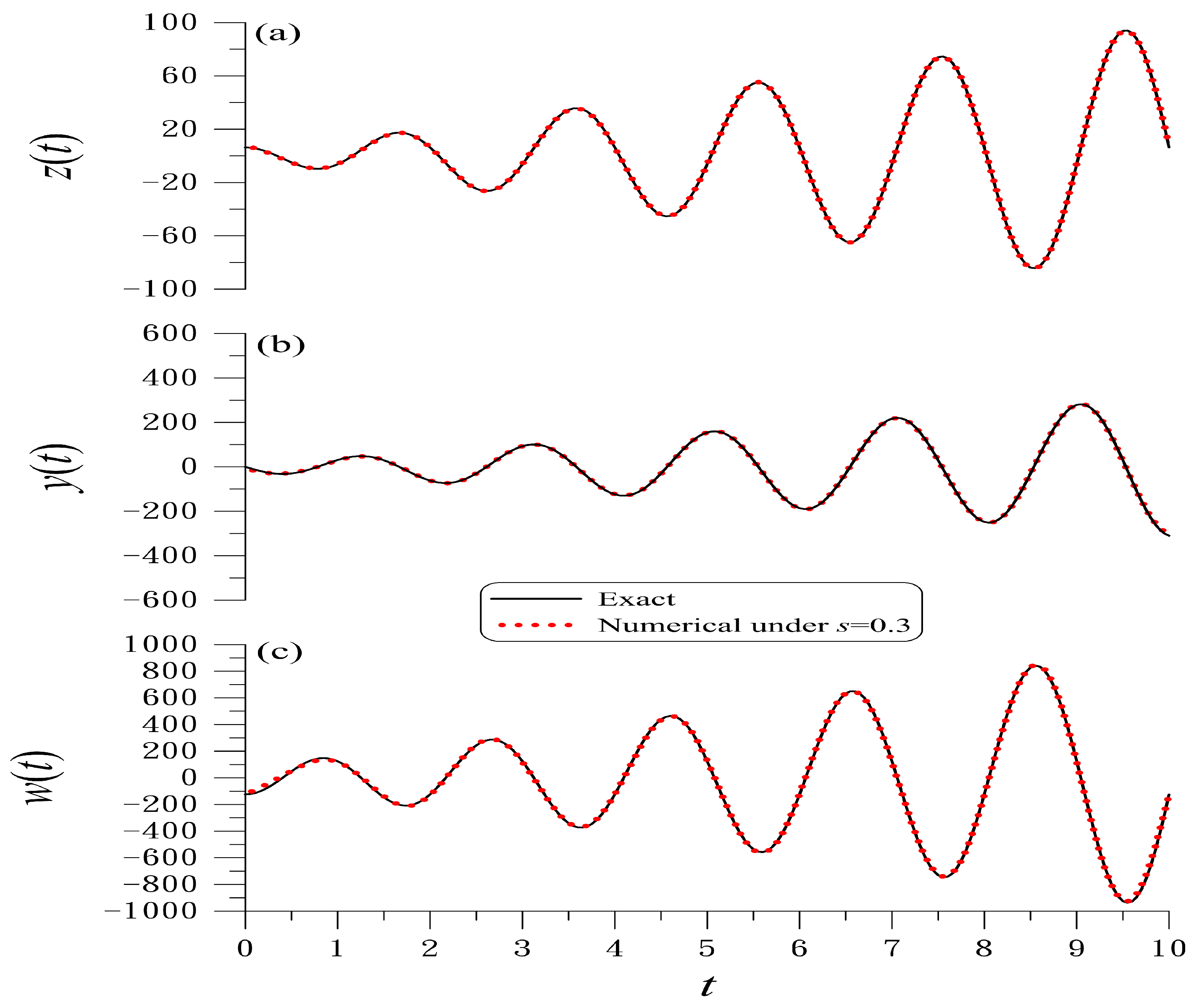
With t f = 10 and s = 0.3 , as shown in Figure 1a–c the recovered derivatives of second-order z ( t ) , third-order y ( t ) , and fourth-order w ( t ) are close to the exact ones, where we take m = 15 , γ = 10076 , and β = 3.2 × 10 11 . For the fourth-order derivative, it can be seen that γ and β are used to reduce the boundary errors to 7.93 × 10 3 , which is very small.
It is interesting that when the accuracy of the fourth-order derivative is improved by using the new WFND, the accuracy of lower-order derivatives is also improved significantly.
In the whole interval, the maximum error of z ( t ) is 1.435, which is much smaller than max | x ¨ ( t ) | = 94.077 . The maximum error of y ( t ) is 8.502, which is much smaller than max | x ( t ) | = 310.063 . The maximum error of w ( t ) is 30.499, which is much smaller than max | x ( 4 ) ( t ) | = 938.206 .

4.2. Example 2

Let
x ( t ) = t 2 / 2 + exp ( sin π t ) , x ˙ ( t ) = t + π cos π t exp ( sin π t ) , x ¨ ( t ) = 1 π 2 sin π t exp ( sin π t ) + ( π cos π t ) 2 exp ( sin π t ) , x ( t ) = π 3 sin 2 π t exp ( sin π t ) [ 3 + sin π t ] / 2 , x ( 4 ) ( t ) = π 4 cos 2 π t exp ( sin π t ) [ 3 + sin π t ] π 4 sin 2 2 π t exp ( sin π t ) / 4 2 π 4 sin 2 π t exp ( sin π t ) cos π t ,
within a time interval t 5 . With s = 0.2 , m = 15 , γ = 3900.38 , and β = 2.023 × 10 12 , Figure 2a–c presents higher-order derivatives which are not as accurate as those in example 1.
As shown in Equation (35), the higher-order derivatives are very complicated. However, the effect of γ and β on reducing the boundary error of the fourth-order derivative is obvious, as shown in Figure 2c, where the boundary errors are 9.45 × 10 5 . Upon comparing with the results obtained by the original weak-form numerical differentiator (WFND) as shown by the dashed-dotted lines in Figure 2 (Figure 9 of [26]), the improvement in accuracy can be seen.

4.3. Example 3

As an engineering application of the new WFND, we apply it to recover an unknown external force of a nonlinear beam equation:
x ( 4 ) ( t ) + x ¨ ( t ) x ( t ) = f ( t ) .
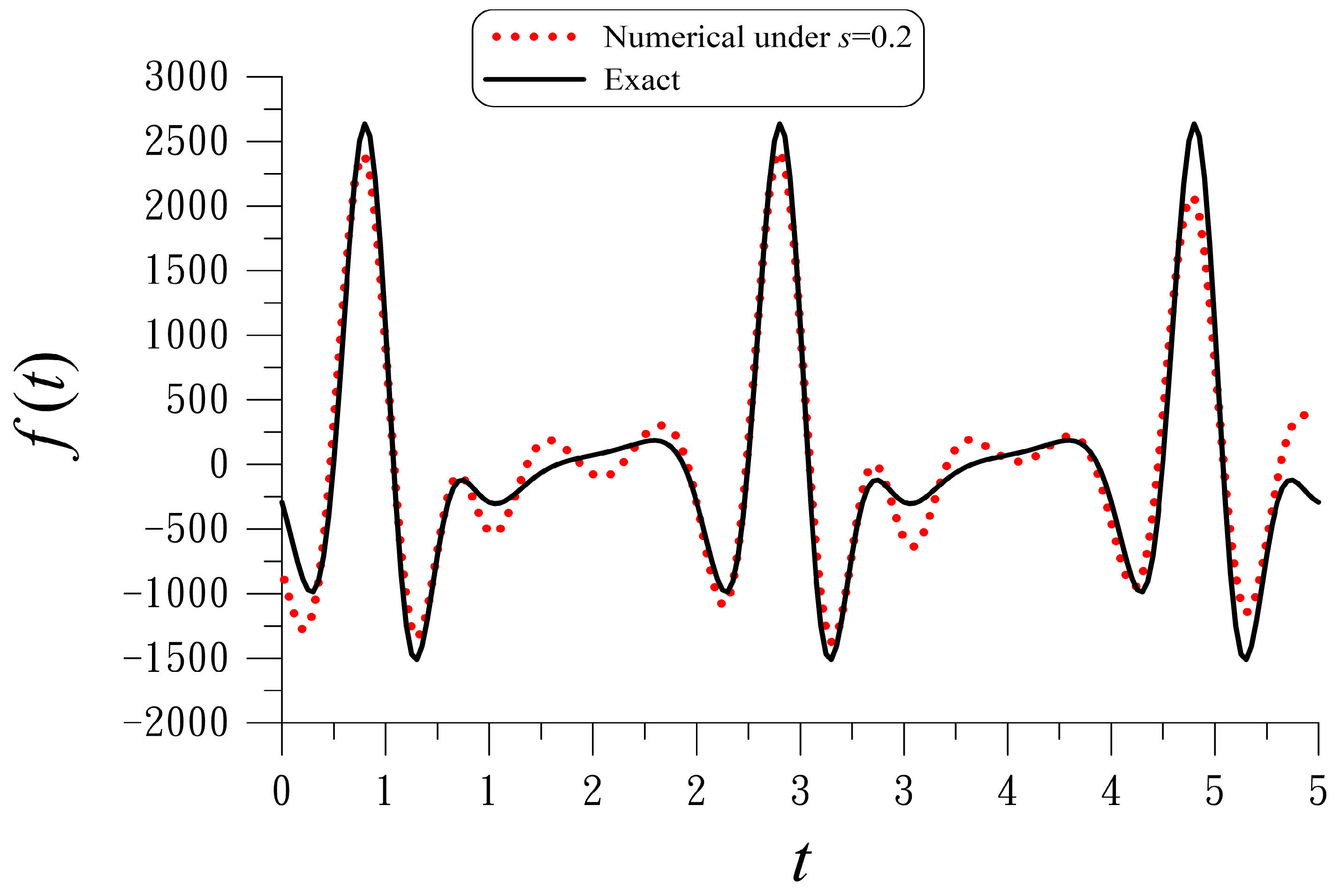
Upon giving the noisy displacement x ^ ( t i ) = [ t i 2 / 2 + exp ( sin π t i ) ] [ 1 + s R ( i ) ] within an interval t 5 , the unknown external force f ( t ) is to be retrieved.
With s = 0.2 , m = 15 , γ = 3900.38 , and β = 0 , we compare the numerically recovered external force to the exact one. The recovered solution of the external force f ( t ) is acceptable, as shown in Figure 3.
Next we consider a nonlinear ODE with a movable singularity [34]:
x ¨ ( t ) = 2 x ( t ) 1 x 2 ( t ) + 1 x ˙ 2 ( t ) ,
whose general solution is
x ( t ) = tan [ ln ( A t B ) ] ,
where A and B are constants. The point B / A is a moving singularity. We take x ( 0 ) = 1 and x ˙ ( 0 ) = 1 , such that A = 1 and B = 1 are fixed.
With m = 15 and t f = 1 , the maximum error of the recovery of the second-order derivative z ( t ) compared to the exact one is 6.614 × 10 3 , which is much smaller than max | x ¨ ( t ) | = 1 .

5. A Linear Beam Equation to Model the Fourth-Order Derivative

In this section, we develop the second method by considering a linear beam equation to model the fourth-order derivative as follows:
u x x x x ( x ) = F ( x ) , 0 < x < ,
which is solvable by subjecting to the boundary conditions:
u ( 0 ) = c 1 , u x x ( 0 ) = c 2 , u ( ) = c 3 , u x x ( ) = c 4 .
Hereon, x denotes the spatial coordinate, u is the displacement of the beam, and the subscript x denotes the derivative with respect to x.
Upon giving a noisy displacement u ^ ( x i ) = u ( x i ) [ 1 + s R ( i ) ] of the beam within an interval 0 x , the unknown external force F ( x ) to be recovered is an approximation of the fourth-order derivative of u ( x ) .

5.1. First Numerical Method

The single-parameter kth-order shape functions p j ( x , k ) , j = 1 , , 4 are determined by
p 1 ( 0 , k ) = 1 , p x x 1 ( 0 , k ) = 0 , p 1 ( , k ) = 0 , p x x 1 ( , k ) = 0 ,
p 2 ( 0 , k ) = 0 , p x x 2 ( 0 , k ) = 1 , p 2 ( , k ) = 0 , p x x 2 ( , k ) = 0 ,
p 3 ( 0 , k ) = 0 , p x x 3 ( 0 , k ) = 0 , p 3 ( , k ) = 1 , p x x 3 ( , k ) = 0 ,
p 4 ( 0 , k ) = 0 , p x x 4 ( 0 , k ) = 0 , p 4 ( , k ) = 0 , p x x 4 ( , k ) = 1 ;
and we can derive [35]
p 1 ( x , k ) = 1 k + 3 2 x k + 2 + k + 1 2 x k + 3 ,
p 2 ( x , k ) = x 2 2 2 4 ( k + 1 ) ( k + 4 ) k + 2 x k + 2 + 2 4 k ( k + 3 ) k + 2 x k + 3 ,
p 3 ( x , k ) = k + 3 2 x k + 2 k + 1 2 x k + 3 ,
p 4 ( x , k ) = 2 2 ( k + 2 ) x k + 3 2 2 ( k + 2 ) x k + 2 ,
where k N with k 1 is a free index.
Then, the following k-parameter boundary shape function
B ( x , k ) = h ( x ) p 1 ( x , k ) [ h ( 0 ) c 1 ] p 2 ( x , k ) [ h x x ( 0 ) c 2 ] p 3 ( x , k ) [ h ( ) c 3 ] p 4 ( x , k ) [ h x x ( ) c 4 ]
automatically satisfies the boundary conditions in Equation (40), where h ( x ) is an arbitrary four-times-differentiable function. It is required that h x x ( 0 ) and h x x ( ) must exist.
We suppose that the displacement can be expanded in terms of B ( x , k ) :
u ( x ) = k = 1 m a k B ( x , k ) ,
where a k are to be determined. For Equation (50), we specify the noisy data u ^ ( x i ) , and by the collocation method it follows that
k = 1 m a k B ( x i , k ) = u ^ ( x i ) , i = 1 , , q ,
where x i , i = 1 , , q are collocated points. Equation (51), together with
k = 1 m a k = 1 ,
leads to n q = q + 1 linear equations to determine the m unknown coefficients a k , k = 1 , , m .
As a consequence of Equations (39) and (50), we can estimate u x x x x ( x ) by
F ( x ) = k = 1 m a k B x x x x ( x , k ) .
The above numerical method to recover the fourth-order derivative represented by the external force F ( x ) will be named the first numerical method (FNM).

5.2. Second Numerical Method

We can also develop the second numerical method (SNM) as follows. For this purpose, we consider four simpler shape functions:
s 1 = 1 x , s 2 = x 3 + x 2 2 x 3 6 , s 3 = x , s 4 = x 6 + x 3 6 .
Then, the following basis function
D ( x , j ) = H ( x , j ) s 1 ( x ) [ H ( 0 , j ) c 1 ] s 2 ( x ) [ H x x ( 0 , j ) c 2 ] s 3 ( x ) [ H ( , j ) c 3 ] s 4 ( x ) [ H x x ( , j ) c 4 ]
automatically satisfies the boundary conditions in Equation (40), where j N is a free index. H ( x , j ) can be any complete basis, for example, H ( x , j ) = ( x / ) j , j = 1 , .
We suppose that the displacement is determined by
u ( x ) = j = 1 m b j D ( x , j ) .
Similarly, by means of Equations (51) and (52), we have n q = q + 1 linear equations to determine the m unknown coefficients b j , j = 1 , , m . Now, by means of of Equations (39) and (56), we can estimate u x x x x by
F ( x ) = j = 1 m b j D x x x x ( x , j ) .
Below, two examples are given to test the performance of FNM and SNM.

5.3. Example 4

The unknown force function F ( x ) is to be recovered from the following example:
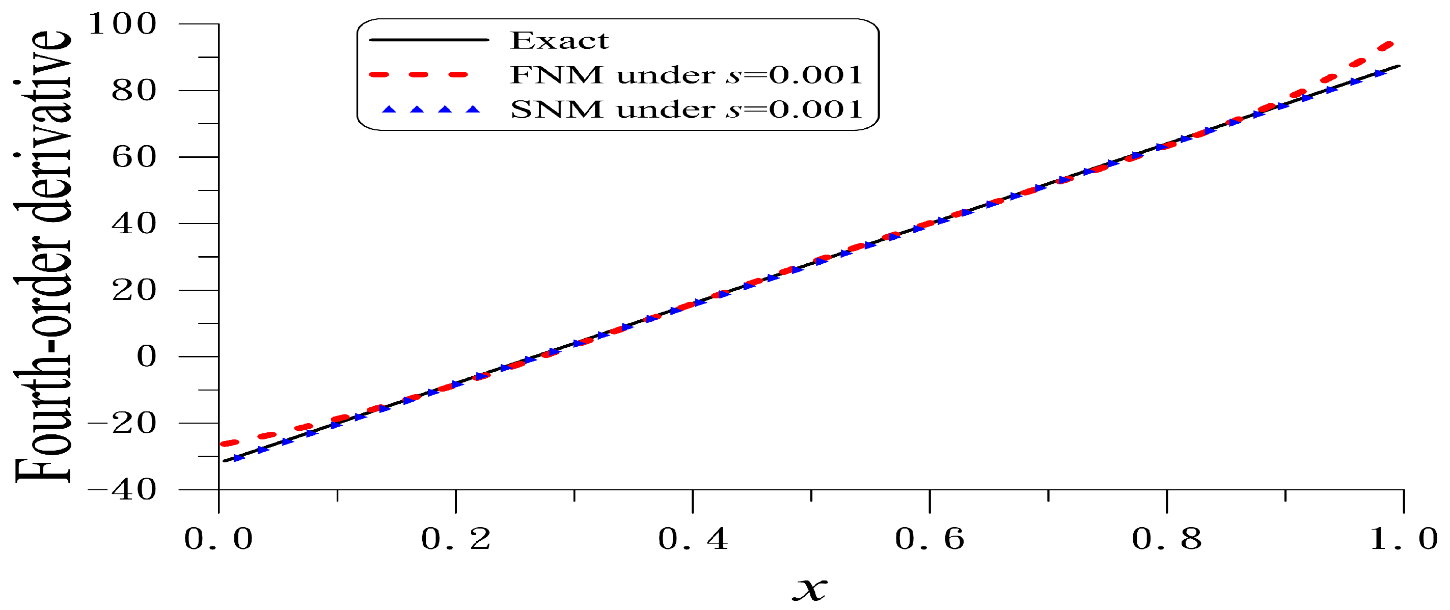
u ( x ) = x 5 4 3 x 4 2 3 x 3 + x , F ( x ) = 120 x 32 .
We take h = 1 + x . With s = 0.001 and m = 6 , the numerically recovered fourth-order derivative is compared to the exact one. The recovered solution obtained by the FNM is acceptable, as shown in Figure 4.
For the SNM, we take H ( x , j ) = ( x / ) j , j = 1 , , m with m = 5 . The recovered solution obtained by the SNM for example 4 is more accurate than that obtained by the FNM, as shown in Figure 4. However, for large noise, both methods cannot obtain a reliable fourth-order derivative of noisy data.

5.4. Example 5

The unknown force function F ( x ) is to be recovered from the following example:
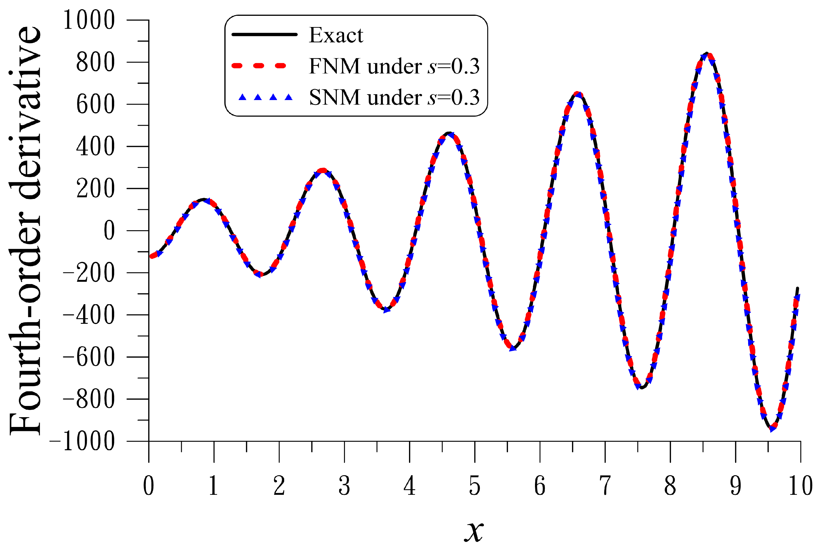
u ( x ) = x sin π x , F ( x ) = 4 π 3 cos π x + π 4 x sin π x .
With h = x sin π x , s = 0.3 , and m = 5 , the numerically recovered external force is compared to the exact one. The recovered solution obtained by the FNM is accurate, as shown in Figure 5.
For this example, we take H ( x , j ) = x j sin j π x , j = 1 , , m and m = 1 in the SNM. Under a noise of s = 0.3 , the numerically recovered fourth-order derivative is compared to the exact one. The recovered solution obtained by the SNM is accurate, as shown in Figure 5.

6. Embedded Method to Compute the Fourth-Order Derivative

In this section, we derive the embedded method and the method of superposition of boundary shape functions (MSBSF) to compute the fourth-order derivative of noisy data.

6.1. Embedded Method

We consider the following linear beam equation:
v x x x x ( x ) = F ( x ) , 0 < x < ,
where the external force F ( x ) to be recovered is the fourth-order derivative of noisy data v ( x ) . Equation (60) is a linear beam model to recover the fourth-order derivative, which is recast to an inverse force problem of a linear beam equation.
Let
u ( x , t ) = e t v ( x )
be a new variable. By using
u t t ( x , t ) = e t v ( x ) ,
and Equation (61), we can immediately obtain
u t t ( x , t ) u ( x , t ) = 0 .
Multiplying Equation (60) by e t yields
e t v x x x x ( x ) = e t F ( x ) ,
which, with the aid of Equation (61), becomes
u x x x x ( x , t ) = e t F ( x ) .
Inserting u t t u , which is zero in view of Equation (62), into Equation (64), we can derive
u t t ( x , t ) + u x x x x ( x , t ) u ( x , t ) = S ( x , t ) , ( x , t ) Ω : = { ( x , t ) 0 < x < , 0 < t t f } ,
u ( x , 0 ) = f ( x ) , u t ( x , 0 ) = h ( x ) , 0 < x < ,
u ( 0 , t ) = 0 , u x x ( 0 , t ) = 0 , u ( , t ) = 0 , u x x ( , t ) = 0 , t [ 0 , t f ] ,
where
S ( x , t ) = e t F ( x ) , f ( x ) = v ( x ) , h ( x ) = v ( x ) .
Although f ( x ) and h ( x ) have the same value of v ( x ) , they play different roles in Equation (66) as f ( x ) is for initial displacement and h ( x ) is for initial velocity. Therefore, we take different notations for them.

6.2. Method of Superposition of Boundary Shape Functions (MSBSF)

We are going to estimate the external force S ( x , t ) for Equation (65), which is a linear Euler–Bernoulli vibrating beam equation with an elastic foundation [36].
To recover S ( x , t ) in Equation (65), the supplementary data are given by
u ( x , t f ) = g ( x ) = e t f v ( x ) ,
u x ( , t ) = ε ( t ) = e t v x ( ) .
Liu et al. [35] employed the method of superposition of boundary shape functions (MSBSF) to recover S ( x , t ) for the linear Euler–Bernoulli beam equations. In Equations (65)–(70), the recovery of S ( x , t ) is quite difficult, because they are under-determined for an inverse force problem. Previously, Liu et al. [37] recovered the unknown spatially dependent forces of the linear Euler–Bernoulli beam equations.
The boundary shape function (BSF) satisfies seven conditions in Equations (66), (67), and (69), including four boundary conditions and three temporal conditions at initial time and final time. We can apply them to the linear beam Equation (65), and introduce a new approach of the inverse force problem of the linear beam equation by using the method of superposition of BSFs (MSBSF).
According to Equations (45)–(48), the following boundary shape functions endowed with a free index k are available [35]:
E ( x , t , k ) = E 0 ( x , t , k ) p 1 ( x , k ) E 0 ( 0 , t , k ) p 2 ( x , k ) E x x 0 ( 0 , t , k )
p 3 ( x , k ) E 0 ( , t , k ) p 4 ( x , k ) E x x 0 ( , t , k ) ,
E ( x , 0 , k ) = f ( x ) , E ( x , t f , k ) = g ( x ) , E t ( x , 0 , k ) = h ( x ) ,
E ( 0 , t , k ) = 0 , E x x ( 0 , t , k ) = 0 , E ( , t , k ) = 0 , E x x ( , t , k ) = 0 .
where p 1 , p 2 , p 3 , p 4 are derived in Equations (45)–(48), and
E 0 ( x , t , k ) = 1 t t f k + 1 f ( x ) + t t f k + 1 g ( x ) + t f t t f t t f k + 1 h ( x ) .
E ( x , t , k ) automatically satisfies the seven conditions in Equations (66), (67), and (69).

7. Numerical Algorithm and Examples

We express the displacement by
u ( x , t ) = k = 1 m a k E ( x , t , k ) .
In Equation (70), we over-specify ε ( t ) = u x ( , t ) to recover S ( x , t ) , such that, from Equation (75), it follows that
k = 1 m a k E x ( , t , k ) = ε ( t ) .
Collocating the discretized times t j , j = 1 , , n in Equation (76) yields
k = 1 m a k E x ( , t j , k ) = ε ( t j ) , j = 1 , , n ,
k = 1 m a k = 1 .
We can determine a k , k = 1 , , m from Equations (77) and (78), and then obtain u ( x , t ) from Equation (75) in the whole domain. Now, after inserting u ( x , t ) into Equation (65), S ( x , t ) can be recovered immediately.
This is a new approach to using MSBSF for the recovery of an unknown external force S ( x , t ) in the linear beam equation with an elastic foundation. It is interesting that with E ( x , t , k ) , k N acting as the bases, only linear equations are used to determine the expansion coefficients by Equations (77) and (78). Numerical examples will show that a small number of bases is sufficient to accurately recover the spatially–temporally dependent external force S ( x , t ) .
We will apply the method presented in Section 6 to compute the fourth-order derivative by using the linear beam model, which is embedded into the system in Equations (65)–(70).
To investigate the robustness of MSBSF, the random noises of R ( x ) [ 1 , 1 ] and R ( t ) [ 1 , 1 ] are imposed on
g ^ ( x ) : = g ( x ) + s R ( x ) , ε ^ ( t ) : = ε ( t ) + s R ( t ) .
In addition, we measure the accuracy of the numerical solution by the maximum error and the relative root-mean-square error:
ME : = max j = 1 , , N | S n ( x j , t j ) S ( x j , t j ) | ,
e ( S ) = j = 1 N [ S n ( x j , t j ) S ( x j , t j ) ] 2 j = 1 N S 2 ( x j , t j ) ,
where S n ( x j , t j ) and S ( x j , t j ) are, respectively, the numerically recovered force and exact force, and ( x j , t j ) , j = 1 , , N are testing points. We fix N = 2500 .
In Equations (68) and (69), f ( x ) , h ( x ) , and u ( x , t f ) are available from v ( x ) by measuring the data of displacements. An extra datum of v x ( ) is required, which is the slope of v ( x ) at the right-end point of the beam. Then we apply MSBSF to recover S ( x , t ) in Equation (65). Inserting t = 0 into S ( x , t ) , we can recover the external force F ( x ) = S ( x , 0 ) in Equation (60), which accounts for the fourth-order derivative of the noisy data v ^ ( x ) . The present technique is embedding the linear beam model in Equation (60) into a vibrating linear beam Equation (65); hence, we name it an embedded method (EM).
The unknown force functions F ( x ) = v x x x x are to be recovered from the following examples:
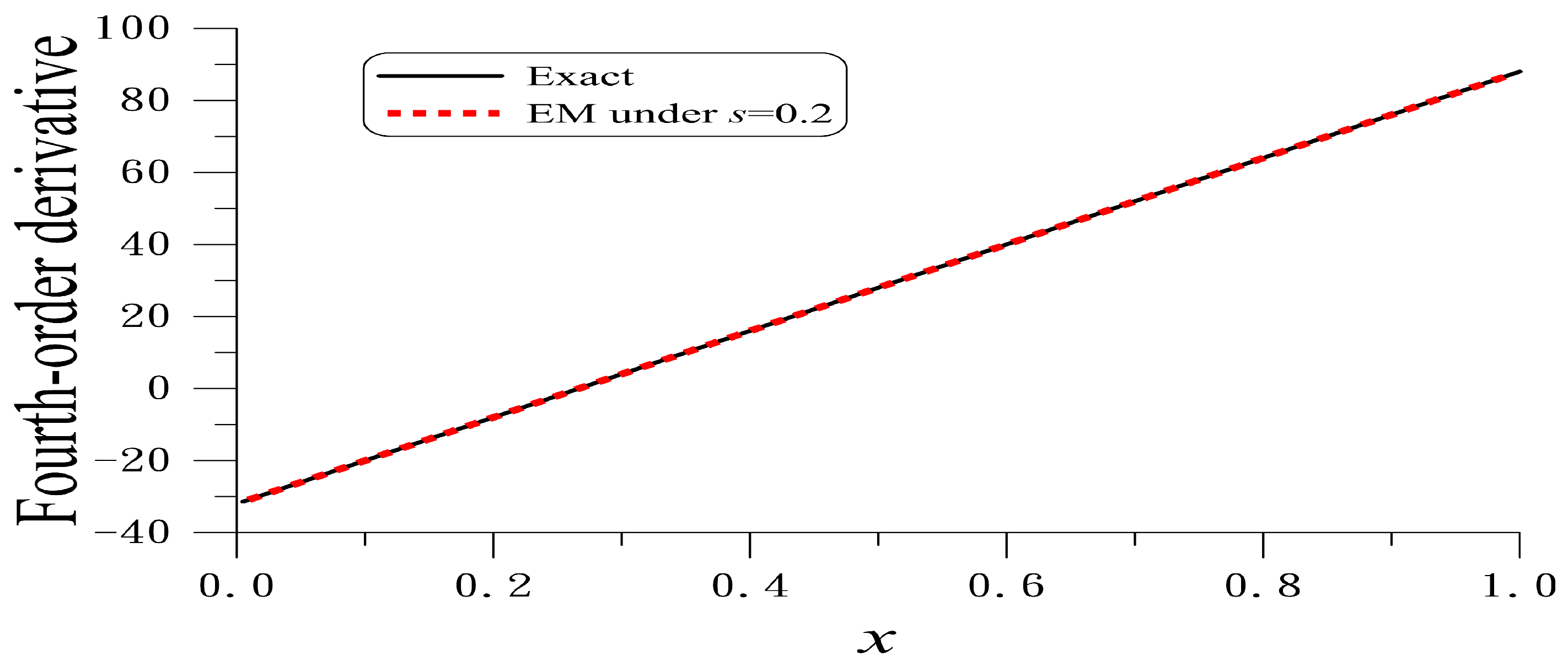
Example   6 : v ( x ) = x 5 4 3 x 4 2 3 x 3 + x ,
Example   7 : v ( x ) = x 4 2 x 3 + x + sin ( π x ) .
We take s = 0.2 , = 1 , and t f = 1 for example 6. With m = 2 , the numerically recovered external force is compared to the exact one in Figure 6. The recovered solution obtained by the EM is very good. The ME to recover the fourth-order derivative F ( x ) is 4.35 × 10 2 , which is much smaller that the maximum value 88 of F ( x ) ; e ( F ) = 6.93 × 10 4 is very small upon comparing to the noise s = 0.2 . Upon comparing to example 4 in Section 5.3, the EM is superior to the FNM and SNM in Section 5. They fail to recover the fourth-order derivative when the noise is large up to s = 0.2 .
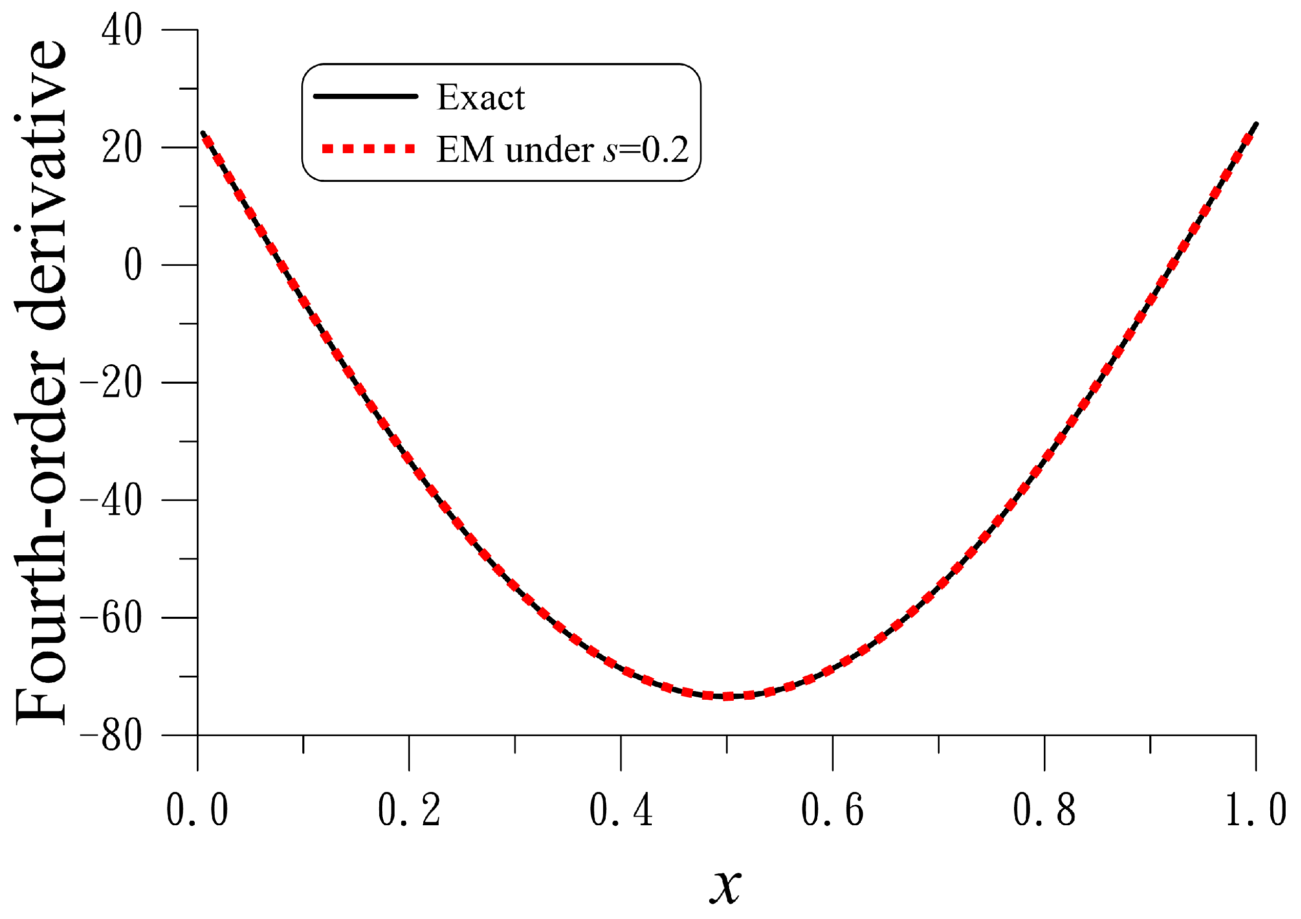
For example 7 with m = 3 , the numerically recovered external force is compared to the exact one in Figure 7, which is very accurate. The ME to recover the fourth-order derivative F ( x ) is 8.5 × 10 3 , which is much smaller that the maximum value 73.41 of F ( x ) ; e ( F ) = 1.31 × 10 4 is very small upon comparing to the noise s = 0.2 .

8. Conclusions

In this paper, we have modified the WFND and proposed a simple numerical method to compute the fourth-order derivatives of noisy data. We can find the fourth-order derivatives directly based on the measured data x ( t ) , not necessarily using the lower-order derivatives of the data x ( t ) . We have proven that there exist two parameters used in the boundary shape function, which can greatly reduce the boundary errors of the fourth-order derivative near to zero. At the same time, we have improved the accuracy of the lower-order derivatives. Three examples confirmed that the new WFND was stable and yet accurate against very large noise up to 20 % and 30 % in the fourth-order numerical derivative of noisy data. Then, we modeled the fourth-order derivative problem as an inverse force problem for a linear beam model. Two collocation numerical methods based on the boundary shape functions were developed to estimate the unknown external force, which is a good approximation of the fourth-order derivative.
We solved the inverse force problem of a linear beam equation with an elastic foundation by adopting MSBSF. Upon substituting the solution into the linear beam equation, we can recover the unknown spatially–temporally dependent force quickly and easily. Finally, we transformed the linear beam model into a system of vibrating linear beam equations by the embedded method (EM). Then, the MSBSF was applied to the embedded system to render very accurate estimations of the fourth-order derivative. Two examples were worked out, which revealed the robustness and accuracy of the EM and MSBSF techniques.
Author Contributions

Conceptualization, C.-W.C.; Methodology, C.-S.L. and C.-W.C.; Validation, C.-S.L. and C.-W.C.; Formal analysis, C.-S.L. and C.-W.C.; Investigation, C.-S.L. and C.-W.C.; Resources, C.-S.L.; Data curation, C.-S.L. and C.-W.C.; Writing—original draft, C.-S.L. and C.-W.C.; Writing—review & editing, C.-S.L. and C.-W.C.; Visualization, C.-W.C.; Supervision, C.-W.C.; Project administration, C.-S.L.; Funding acquisition, C.-S.L. All authors have read and agreed to the published version of the manuscript.

Funding

The NSTC 113-2221-E-019-043-MY3 granted by the National Science and Technology Council, who partially supported this study, is gratefully acknowledged.

Institutional Review Board Statement

Not applicable.

Informed Consent Statement

Not applicable.

Data Availability Statement

The data presented in this study are available on request from the corresponding author.

Conflicts of Interest

The authors declare no conflicts of interest.

References

  1. Liu, C.S.; Atluri, S.N. A GL(n,ℝ) differential algebraic equation method for numerical differentiation of noisy signal. Comput. Model. Eng. Sci. 2013, 92, 213–239. [Google Scholar]
  2. Hanke, M.; Scherzer, O. Inverse problems light: Numerical differentiation. Amer. Math. Mon. 2001, 108, 512–521. [Google Scholar] [CrossRef]
  3. Ramm, A.; Smirnova, A.B. On stable numerical differentiation. Math. Comput. 2001, 70, 1131–1153. [Google Scholar] [CrossRef]
  4. Ahn, S.; Choi, U.J.; Ramm, A.G. A scheme for stable numerical differentiation. J. Comput. Appl. Math. 2006, 186, 325–334. [Google Scholar] [CrossRef]
  5. Wang, X.; Shirinzadeh, B. High-order nonlinear differentiator and application to aircraft control. Mech. Sys. Sign. Process. 2014, 46, 227–252. [Google Scholar] [CrossRef]
  6. Tang, J.; Lu, J. Modified extended Lie-group method for Hessenberg differential algebraic equations with index-3. Mathematics 2023, 11, 2360. [Google Scholar] [CrossRef]
  7. Shmaliy, Y.S.; Zhao, S.; Ahn, C.K. Kalman and UFIR state estimation with coloured measurement noise using backward Euler method. IET Signal Proc. 2020, 14, 64–71. [Google Scholar] [CrossRef]
  8. Michel, L.; Ghanes, M.; Plestan, F.; Aoustin, Y.; Barbot, J.P. Semi-implicit homogeneous Euler differentiator for a second-order system: Validation on real data. In Proceedings of the 2021 60th IEEE Conference on Decision and Control (CDC), Austin, TX, USA, 14–17 December 2021; pp. 5911–5917. [Google Scholar]
  9. Xu, A.; Cen, Z. A remainder formula of numerical differentiation for the generalized Lagrange interpolation. J. Comput. Appl. Math. 2009, 230, 418–423. [Google Scholar] [CrossRef]
  10. Bai, H.; Xu, A.; Cui, F. Representation for the Lagrangian numerical differentiation formula involving elementary symmetric functions. J. Comput. Appl. Math. 2009, 231, 907–913. [Google Scholar] [CrossRef]
  11. Zhang, Y.; Jin, L.; Guo, D.; Yin, Y.; Chou, Y. Taylor-type 1-step-ahead numerical differentiation rule for first-order derivative approximation and ZNN discretization. J. Comput. Appl. Math. 2015, 273, 29–40. [Google Scholar] [CrossRef]
  12. Othmane, A.; Rudolph, J.; Mounier, H. Systematic comparison of numerical differentiators and an application to model-free control. Euro. J. Contr. 2021, 62, 113–119. [Google Scholar] [CrossRef]
  13. Levant, A.; Livne, M.; Yu, X. Sliding-mode-based differentiation and its application. IFAC-PapersOnLine 2017, 50, 1699–1704. [Google Scholar] [CrossRef]
  14. Kikuuwe, R.; Pasaribu, R.; Byun, G. A first-order differentiator with first-order sliding mode filtering. IFAC-PapersOnLine 2019, 52, 771–776. [Google Scholar] [CrossRef]
  15. Deepika, D. Frameworks for double hyperbolic function-based robust sliding mode differentiator and observer for nonlinear dynamics. Asian J. Contr. 2022, 24, 273–281. [Google Scholar] [CrossRef]
  16. Djennoune, S.; Bettayeb, M.; Al-Saggaf, U.M. Fixed-time convergent sliding-modes-based differentiators. Commun. Nonl. Sci. Numer. Simul. 2022, 104, 106033. [Google Scholar] [CrossRef]
  17. Li, J. General explicit difference formulas for numerical differentiation. J. Comput. Appl. Math. 2005, 183, 29–52. [Google Scholar] [CrossRef]
  18. Dutt, A.; Gu, M.; Rokhlin, V. Fast algorithms for polynomial interpolation, integration, and differentiation. SIAM J. Numer. Anal. 1996, 33, 0733082. [Google Scholar] [CrossRef]
  19. Dell’Accio, F.; Di Tommaso, F.; Siar, N.; Vianello, M. Numerical differentiation on scattered data through multivariate polynomial interpolation. BIT Numer. Math. 2018, 62, 773–801. [Google Scholar] [CrossRef]
  20. Nayak, A. A new regularization approach for numerical differentiation. Inv. Prob. Sci. Eng. 2020, 28, 1747–1772. [Google Scholar] [CrossRef]
  21. Chen, B.; Zhao, Z.; Li, Z.; Meng, Z. Numerical differentiation by a Fourier extension method with super-order regularization. Appl. Math. Comput. 2018, 334, 1–10. [Google Scholar] [CrossRef]
  22. Zhao, Z.; You, L. A numerical differentiation method based on Legendre expansion with super order Tikhonov regularization. Appl. Math. Comput. 2021, 393, 125811. [Google Scholar] [CrossRef]
  23. Davydov, O.; Schaback, R. Error bounds for kernel-based numerical differentiation. Numer. Math. 2016, 132, 243–269. [Google Scholar] [CrossRef]
  24. Egidi, N.; Maponi, P. The singular value expansion of the Volterra integral equation associated to a numerical differentiation problem. J. Math. Anal. Appl. 2018, 460, 656–681. [Google Scholar] [CrossRef]
  25. Egidi, N.; Giacomini, J.; Maponi, P.; Youssef, M. An FFT method for the numerical differentiation. Appl. Math. Comput. 2023, 445, 127856. [Google Scholar] [CrossRef]
  26. Liu, C.S.; Dong, L. Closed-form higher-order numerical differentiators for differentiating noisy signals. Appl. Math. Comput. 2019, 359, 386–403. [Google Scholar] [CrossRef]
  27. Duan, F.; Wang, J.J. A regularization method for delivering the fourth-order derivative of experimental data and its applications in fluid-structure interactions. Sci. China Techn. Sci. 2025, 68, 1321101. [Google Scholar] [CrossRef]
  28. Richard, M.C. Mechanics of Composite Materials, 1st Version; John Wiley and Sons: New York, NY, USA, 1979. [Google Scholar]
  29. Robert, J.M. Mechanics of Composite Materials, 1st Version; Hemisphere: New York, NY, USA, 1975. [Google Scholar]
  30. Abu-Hilal, M. Forced vibration of Euler-Bernoulli beams by means of dynamic Green functions. J. Sound Vib. 2003, 267, 191–207. [Google Scholar] [CrossRef]
  31. Nicaise, S.; Zair, O. Determination of point sources in vibrating beams by boundary measurements: Identifiability, stability, and reconstruction results. Electron. J. Differ. Equ. 2004, 20, 1–17. [Google Scholar]
  32. Liu, C.S. A Lie-group adaptive differential quadrature method to identify unknown force in an Euler-Bernoulli beam equation. Acta Mech. 2012, 223, 2207–2223. [Google Scholar] [CrossRef]
  33. Hasanov, A.; Baysal, O. Identification of unknown temporal and spatial load distributions in a vibrating Euler-Bernoulli beam from Dirichlet boundary measured. Automatica 2016, 71, 106–117. [Google Scholar] [CrossRef]
  34. Sachdev, P.L. Nonlinear Ordinary Differential Equations and Their Applications; Marcel Dekker Inc.: New York, NY, USA, 1991. [Google Scholar]
  35. Liu, C.S.; Kuo, C.L.; Chang, C.W. Recovering external forces on the vibrating Euler-Bernoulli beams by the methods of boundary shape functions. Mech. Sys. Sig. Proc. 2021, 148, 107157. [Google Scholar] [CrossRef]
  36. Fertis, D.G. Nonlinear Mechanics; CRC Press: London, UK, 1993. [Google Scholar]
  37. Liu, C.S.; Jhao, W.S.; Chang, C.W. A simple non-iterative method for recovering a space-dependent load on the Euler-Bernoulli beam equation. Math. Meth. Appl. Sci. 2018, 41, 7641–7654. [Google Scholar] [CrossRef]
Figure 1. Showing and comparing second-order to fourth-order numerical derivatives to the exact ones in (ac) of example 1.
Eng 06 00324 g001
Figure 2. Showing and comparing second-order to fourth-order numerical derivatives to the exact ones in (ac) of example 2.
Eng 06 00324 g002
Figure 3. For a nonlinear beam equation in example 3 comparing numerical and exact external forces.
Eng 06 00324 g003
Figure 4. For example 4, a linear beam model to recover the fourth-order derivative by comparing numerical and exact ones.
Eng 06 00324 g004
Figure 5. For example 5, a linear beam model to recover the fourth-order derivative by comparing numerical and exact ones.
Eng 06 00324 g005
Figure 6. For example 6, a linear beam model to recover the fourth-order derivative by comparing numerical result recovered by the embedded method (EM) and the exact fourth-order derivative.
Eng 06 00324 g006
Figure 7. For example 7, a linear beam model to recover the fourth-order derivative by comparing numerical result recovered by the embedded method (EM) and the exact fourth-order derivative.
Eng 06 00324 g007
Disclaimer/Publisher’s Note: The statements, opinions and data contained in all publications are solely those of the individual author(s) and contributor(s) and not of MDPI and/or the editor(s). MDPI and/or the editor(s) disclaim responsibility for any injury to people or property resulting from any ideas, methods, instructions or products referred to in the content.