Abstract
Accurate estimation of the mean fragment size is crucial for optimizing open-pit mining operations. This study presents an approach that combines clustering, hyperparameter optimization, and data augmentation to enhance prediction accuracy using the Xtreme Gradient Boosting (XGBoost) regression model. A dataset of 110 blasts was divided into 97 blasts for training and testing, whereas a separate set of 13 new, unseen blasts was used to evaluate the robustness and generalization of the model. Hierarchical Agglomerative (HA) and K-means clustering algorithms were used, with HA clustering providing a higher cluster quality. To address class imbalance and improve model generalization, a synthetic minority oversampling technique for regression with Gaussian noise (SMOGN) was employed. Hyperparameter tuning was conducted using HyperOpt by comparing Random Search (RS) with the Advanced Tree-structured Parzen Estimator (ATPE). The combination of ATPE with HA clustering and SMOGN in an expanded search space produced the best results, achieving superior prediction accuracy and reliability. The proposed HAC1-SMOGN model, which integrates HA clustering, ATPE tuning, and SMOGN augmentation, achieved a mean squared error (MSE) of 0.0002 and an R2 of 0.98 on the test set. This study highlights the synergistic benefits of clustering, hyperparameter optimization, and data augmentation in enhancing machine learning models for regression tasks, particularly in scenarios with class imbalance or limited data.
1. Introduction
Predicting the mean fragment size (50% passing size) in rock blasting is a critical component of mining operations because it directly affects downstream processes such as loading, hauling, and crushing [1,2]. Accurate predictions enable better planning and cost management, thereby enhancing the operational efficiency and safety [3]. However, the inherent complexity and variability of geological formations pose significant challenges for achieving precise predictions. Traditional empirical methods often fall short because of their inability to capture complex patterns and interactions within data [4]. This has led to increased interest in applying machine learning techniques to improve prediction accuracy [5].
Machine learning offers a promising alternative, as it can leverage large datasets to uncover hidden patterns and relationships that traditional methods may overlook. Bahrami et al. [6] demonstrated that an Artificial Neural Network (ANN) architecture utilizing a back-propagation algorithm over multi-variate analysis (MVA) was a competent measure for predicting rock fragmentation in the Sangan Iron ore mine. Shi et al. [7] compared Support Vector Machines (SVMs), ANN, MVA, and conventional Kuznetsov methods. The study showed that machine learning methods have a better prediction accuracy than traditional methods. Miao et al. noted that at the Dexing Copper Mine in China, [8] the SVM regression model yielded good prediction accuracy, high precision, and robust generalization ability. Among the various machine learning models, Extreme Gradient Boosting (XGBoost) has gained popularity in the field of rock blasting, owing to its high performance and robustness in handling diverse datasets. Nabavi et al. [9] demonstrated the superior overall performance of the XGBoost hybrid model for predicting blast-induced back breaks in the Chadormalu mine (Iran). The model outperformed other hybrid models, namely Random Forest (RF), gene expression programming (GEP), linear multiple regression (LMR) and nonlinear multiple regression (NLMR). Zhang et al. [10] used XGBoost as the principal model for predicting blast-induced PPV and integrated Particle Swarm Optimization (PSO), leading to an accuracy of 96.1% compared with the best empirical technique, with an accuracy (VAF) of only 54.5%. Chandrahas et al. assessed K Nearest neighbors (KNN), XGBoost, and RF and realized that the predicted values from XGBoost closely mirrored the measured values of PPV and fragmentation. Nonetheless, the performance of machine learning models is highly dependent on the selection of appropriate hyperparameters. Hyperparameter optimization, which largely depends on the tuning technique employed, is crucial for enhancing model performance, and several techniques have been proposed to address this need. Amoako et al. [11] used Grid Search and Bayesian Optimization for hyperparameter tuning with SVR and a multilayered ANN to estimate the mean fragment size. Both the models outperformed the conventional Kuznetsov model. Xie et al. [12] used a hybrid machine learning technique combining a firefly algorithm (a metaheuristic) with a Gradient Boosting Machine (GBM), ANN, SVM and Gaussian Process (GP). The study concluded that the FFA-GBM presented the highest computational stability and efficiency. Jia et al. [13] employed a grey wolf optimizer (GWO) to optimize an extreme learning machine (ELM) to predict the mean fragmentation size at an open-pit coal mine.
In this study, we applied Random Search (RS) and Adaptive Tree-structured Parzen Estimator (ATPE) as search optimization algorithms (SOAs). Random Search is one of the simplest and most widely used hyperparameter optimization techniques. This involves the random sampling of the hyperparameter space to determine the optimal configuration. However, recent advancements have introduced more sophisticated methods such as ATPE. ATPE is a Bayesian optimization technique that models the hyperparameter space and adaptively adjusts the search strategy based on previous results, potentially offering more efficient and effective optimization than Random Search.
In addition to hyperparameter optimization, clustering techniques can be employed to improve the model performance by grouping similar data points. Hierarchical Agglomerative (HA) clustering and K-means clustering are two commonly used methods. HA builds a hierarchy of clusters by progressively merging or splitting existing clusters, whereas K-means partitions data into a specified number of clusters by minimizing the variance within each cluster. By clustering the dataset, we can tailor the model to capture the specific characteristics of each group better, potentially leading to more accurate predictions. Hudaverdi et al. [14] applied hierarchical clustering to generate data clusters based on the elastic moduli of intact rock. Clustering resulted in two multi-variate regression analysis (MVRA) equations for predicting the blast fragmentation distribution. Nguyen et al. [15] concluded that combining Hierarchical K-means clustering and the cubist algorithm (CA) led to a superior model owing to the excellent accuracy of the PPV predictions. Sheykhi et al. [16] evaluated SVR standalone and hybrid fuzzy C-means clustering (FCM)–SVR for blast-induced ground vibrations. The study concluded that data clustering has a significant impact on the prediction accuracy.
However, one of the challenges faced in clustering is dealing with imbalanced datasets. For instance, in our study, Cluster 1 (C1) contained significantly fewer data points than Cluster 2 (C2). This imbalance can lead to biased models that do not generalize well [17]. To address this, a data augmentation technique, namely synthetic minority oversampling technique for regression with Gaussian noise (SMOGN version 0.1.2), was applied. SMOGN generates synthetic data points for the minority class, thereby balancing the dataset and improving the generalization ability of the model.
Despite the benefits associated with clustering and data augmentation, limited research exists, particularly in the field of rock blasting, where features exhibiting complex relationships and data size limitations are also a common phenomenon.
This study presents a step-by-step approach to combining these techniques to build robust models. The initial phase was aimed at evaluating the effectiveness of RS and ATPE as hyperparameter optimization techniques for predicting mean fragment size using XGBoost. Next, the impact of clustering using HA and K-means clustering is investigated. Finally, SMOGN is applied to Cluster 1, which consists of minority classes. By comparing the performance of the models across different configurations, we aimed to identify the best clustering technique, optimal hyperparameter optimization method, associated influential hyperparameters, and the influence of search space on model performance.
2. Materials and Methods
In this section, we provide an overview of the machine learning models and clustering techniques employed and present the dataset used in this study to predict the mean fragmentation size.
2.1. Dataset
The dataset comprised 110 blasts. Using this dataset, we developed an XGBoost model that used Hyperopt for hyperparameter tuning to predict the mean fragment sizes of muckpiles during mine blasting. The objective was to assess the impact of clustering based on the selected clustering techniques.
The compilation of the dataset was performed by Hudaverdi et al. [14]. The dataset was compiled from previous studies conducted in mines around the world. For example, the Mi symbol represents the Pinal Schist quarry in Arizona, USA. En, Rc, and Ru represent data from the Enusa and Reocin mines in Spain. The symbols represent various mines. These mines include open-pit uranium mines, copper mines (Mg), zinc mines, coal mines (Sm), manganese mines, and quarries (Ad, Oz). The rock formations also differed depending on the location and type of target ore. Thus, it ranges from dacite, andesite, micaceous schist, and muscovite schist, to moderately to heavily folded schistose.
The diversity of the data meant that an array of rock formations, including the blast design parameters, were available for analysis. However, according to Hudaverdi et al. [14], only the parameters that were common across all blasts were selected. The dataset includes rock, geometric, and explosive parameters, all of which represent the three key factors that affect rock fragmentation. These included burden, hole depth, stemming length, spacing, and hole diameter. As shown in Table 1, four geometric features of the seven input parameters were represented in ratio form to better understand their relationships and impact on fragmentation quality. These include the ratio of stemming to burden (T/B), burden to hole diameter (B/D), and bench height to drilled burden (H/B), which acts as a stiffness ratio, and spacing to burden (S/B), which is fundamental in determining the energy distribution in a rock mass. Powder Factor (PF) represents the explosive property. The rock mass structure expressed by XB indicates the intact rock prior to blasting, while the modulus of elasticity ‘E’ is a geo-mechanical parameter that represents the rock property.

Table 1.
Dataset statistics.
The objective of Hudaverdi et al. [14] was to establish a fragmentation prediction model based on a multivariate analysis. The target variable was the mean fragment size. The size of the mean fragment varied significantly because the data were sourced from different mines located in different parts of the world with distinctive geological conditions and blasting standards. Image analysis softwares were used to measure the mean fragment sizes based on the most popular fragmentation model, that is, the Kuznetsov equation adapted by Cunningham [18].
where
is the mean fragment size (cm), A is the rock factor, K is the powder factor (kg/m3), Q is the mass of the explosive being used (kg), Sanfo is the weight strength relative to ANFO, and 115 is the relative weight strength of TNT.
Other researchers have used the same dataset for machine learning. For example, Shi et al. proved that the prediction accuracy of the SVM model was better than that of the multivariate regression analysis (MVRA). Kulatilake et al. used traditional artificial neural networks (ANNs) and MVRA to predict mean fragment size. Amoako et al. assessed the potential of multi-layered ANN and SVR and utilized Grid Search for SVR and Bayesian Optimization for ANN.
A statistical summary of the data is outlined in Table 1 and Figure 1 (see the original data in Table A1 in the Appendix A).

Figure 1.
Correlations between input parameters and output parameter.
Figure 2 shows the relationship between the specific charge and the mean fragment size of the 12 monitored blasts, whose symbol is ‘Mr’ and forms part of the dataset [19].
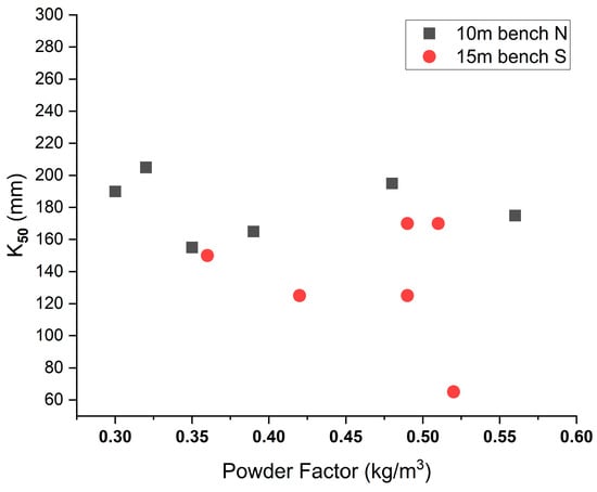
Figure 2.
Mean fragment size (K50) vs. specific charge for 12 blasts (Mr1-Mr12) at Mrica.
2.2. Machine Learning Algorithm
In this section, we discuss the machine learning algorithms utilized in this study. The Xtreme Gradient Boosting (XGBoost version 1.7.6) regression method forms the basis of this investigation. It was tuned using the Hyperopt library and by applying either a Random Search or an Adaptive Tree-structured Parzen Estimator (ATPE). The Python library, Windows 11, 64-bit OS, 32 gb RAM, and 11th Gen i5 comprise the computing environment. An overview of these methods is provided below.
2.2.1. XGBoost
It is a supervised machine learning model developed by Chen and Guerin [20]. This is an effective tree-based ensemble learning algorithm that uses a gradient boosting method. It combines multiple ‘weak’ or foundational learners to improve prediction efficiency [21]. Any tree added aims to correct prediction errors associated with a previous series of weak learners. XGBoost is briefly outlined as follows [22].
where
denotes the predicted value, F denotes the basic model, and M denotes the number of trees.
The objective function (L) is outlined below:
The objective function above is a representation of the loss function, that is, the difference between the actual and predicted values, and a regularization term () is added to address the complexity of the model and prevent overfitting.
where T is the number of leaves, γ is a regularization parameter for penalizing the number of leaves in the trees, λ is for penalizing large weights in the regression tree, and
represents the sum of squares of the weights of the leaves, which helps prevent assignment bias to the importance of any single feature or a set of features.
A Taylor expansion was applied to the loss objective function to promote efficient computation and improve the convergence [23].
Overfitting was prevented by managing tree overgrowth. This is controlled by the addition of the splitting threshold γ. The splitting of the leaf node is allowed only once the threshold value is less than that of the information gain. In addition, proper tuning of the parameters is essential for controlling model complexity.
2.2.2. Hyperopt Library for Hyperparameter Tuning
Hyperopt is an open-source library in Python that is explicitly used to optimize machine learning pipelines and model hyperparameters. The three essential steps of the Hyperopt functionality are defining the objective function, defining the search space, and selecting the search algorithm [24]. In this study, the traditional Random Search algorithm and Adaptive Tree-structured Parzen Estimator (ATPE), a modern form of Bayesian Optimization within the Hyperopt library, were assessed.
The following is a summary of search algorithms.
2.2.3. Random Search
This is an example of a naive optimization algorithm, that is, a simplistic and straightforward algorithm. According to Bergstra and Bengion [25], Random Search (RS) can be used as a natural baseline to gauge the performance of sophisticated models. The same study further demonstrated that Random Search, also known as random sampling, randomly explores the hyperparameter space and enables a more comprehensive search than other techniques such as grid search, which limits the search to a specific grid. Consequently, with fewer iterations, a Random Search can find a good solution in less computational time, particularly if the best solutions lie outside the predefined grid, as in the grid-search example. Additionally, it is more efficient in high-dimensional spaces. The number of iterations significantly affected the effectiveness of this technique. This was the basis for choosing Random Search as the standard model in our study.
2.2.4. Adaptive Tree-Structured Parzen Estimator (ATPE)
The Tree-structured Parzen Estimator (TPE) is a variant of Bayesian Optimization methods. It is referred to as ‘tree-structured’ because it handles conditional parameters that create a tree-like search space. It uses a Parzen window or kernel density estimator (KDEs) to create probability density functions in a hyperparametric search space [26]. TPE can construct a search space with a discrete or quantized uniform distribution, logarithmic uniform distribution, or uniform distribution, which presents a level of flexibility [27]. In addition, as a global optimization algorithm that uses sequential modeling, TPE has proven to be robust in handling conditional parameters, such as the learning rate and maximum depth. Thus, TPE overcomes the limitations associated with conventional Bayesian Optimization methods.
TPE works by modeling p(x∣y) and p(y) to reduce computation. It uses a truncated Gaussian mixture to model the prior distributions of each parameter, and updates them based on subsequent observations.
It then sorts the target values and splits y into two segments, using y∗ as the dividing boundary. The conditional probability density function (PDF) of x, given y, is subsequently established for each segment.
where
is the density formed by observation
which is greater than
and
is the density formed by the remaining observations [28].
Therefore, ATPE is an enhanced variant of the TPE. While TPE adopts a static approach with fixed strategies for balancing exploration and exploitation, ATPE, on the other hand, has an adaptive mechanism, that is, it can dynamically adjust exploration and exploitation based on search progress, leading to faster convergence owing to increased search efficiency. It is also more efficient than the standard TPE, especially for larger and more complex search spaces.
For the XGBoost model, such as that employed in this study, the role of the ATPE is to optimally search for the parameters associated with the main model, that is, the learning rate, max depth, subsample, n_estimators, min_child_weight, and colsample_bytree. The role of each parameter is crucial. For example, the learning rate controls how the model is trained by determining the step size at each iteration. N estimators are responsible for the number of trees to be used; the maximum depth determines how deep a tree can grow, which helps capture complex interactions between features.
2.3. Clustering Techniques
The objective of clustering is to achieve a high similarity within a class and a low similarity between classes. Clustering refers to the classification of data by identifying the features within a dataset that can describe their correlation or differentiation. The three main data-clustering techniques are partitioning, hierarchical clustering, and density-based clustering. In our study, we evaluated hierarchical clustering using an agglomerative approach and K-means clustering on our original dataset, that is, 97 blasts prior to preprocessing.
2.3.1. Hierarchical Agglomerative Clustering (HAC)
In HA, different data points are linked to form a branch in a tree representation of distance [29]. Therefore, HA clustering builds a tree-like cluster structure within the dataset. This tree-like structure, represented by the dendrogram in Figure 3, allows each node to represent a cluster of data points. This representation does not require a pre-definition of the number of clusters, which is common in partition-based clustering, thus making it more versatile for implementing and extracting insights. Agglomerative clustering initializes each data point as a cluster [30]. In this study, the Euclidean distance metric and Pearson Correlation Distance (PDC) were used to compute pairwise distances between data points. Euclidean distance is based on geometric distances in space, whereas correlation distance uses a correlation coefficient to capture the similarity of patterns between variables rather than absolute distances in space. Different linkage criteria were also used to check similarity by computing pairwise distances between clusters. Table 2 lists the performances based on the applied linkage criteria. To achieve the desired number of clusters, that is, segmentation of our dataset into a cluster size that would provide a desirable data size for machine learning, we cut our dendrogram at a height of 200, thus availing two clusters for our analysis (Figure 3).
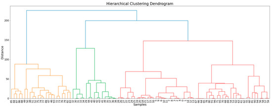
Figure 3.
A dendrogram of blast samples showing hierarchical agglomeration separation using PDC.

Table 2.
Outcome of HA clustering based on linkage criteria.
Table 2 presents the results of data classification based on the following Hierarchical Agglomeration methods: Ward, Single, Average, Complete and the Pearson Correlation Distance (PDC) output. The best cluster output was produced by the PDC. Although the original study only focused on the PDC, the results of this study were congruent with the earlier results of Hudaverdi et al. [14]. The groupings of the original data were (35 for Group 1 and 62 for Group 2). This justifies the use of PDC with the average linkage method as the best method.
2.3.2. K-Means Clustering
K-means clustering is a partition-based clustering method. It is commonly applied because of its simplicity. In K-means, the optimum number of K, which defines the number of predefined clusters and the centroid location of the cluster to maximize the intercluster variance between groups and minimize intracluster variance within the groups, is obtained through an iterative process. This technique was also assessed for its suitability to our dataset. The K-means class from Scikit-learn was implemented using Euclidean distance to assign data points to the nearest cluster centroids. The elbow and silhouette methods were used to determine the optimal value of K to avoid ambiguity, which is often associated with the identification of elbow points in the Elbow Method [31].
As shown in Figure 4, the elbow method stipulates that the optimal K is found within a range of four to seven clusters. From both the elbow and silhouette graphs, we can conclude that any cluster size between four and seven optimal K values yields satisfactory results when compared with the two clusters. To provide further insight into the comparison of clustering, Figure 5 shows the clustering of our dataset into two and four clusters. Based on the average silhouette coefficient value, although four clusters with an average silhouette score of 0.32 perform better than two clusters with a silhouette score of 0.12 (indicative of moderate clustering quality), machine learning is sensitive to the data size; therefore, the smallest possible cluster was chosen in order to maintain a reasonable data size to prevent intense data imbalance for model training and testing.
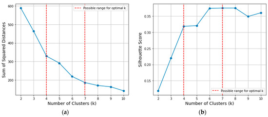
Figure 4.
(a) Elbow Method for optimal K and (b) Silhouette Score for optimal K.
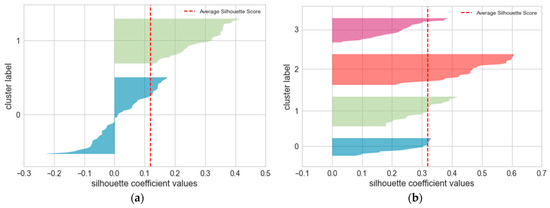
Figure 5.
Silhouette plots for K-means clustering: (a) 97 samples in 2 centers; (b) 97 samples in 4 centers.
2.3.3. Other Clustering Techniques
Alternative clustering techniques were used to justify the selection of the HA and K-means clustering. The results are presented in Table 3.

Table 3.
Comparing the performance of other clustering techniques.
From the above results, it is evident that Gaussian Mixture Models (GMMs) can be used to validate HA clustering and K-means clustering based on the proportion of data points.
2.3.4. Mean Vector Variables
This section displays the mean vectors of the two groups generated by HA, K-means, and GMM through feature comparison. The magnitude of the differences in the mean values indicates the extent of divergence or disparity between variables. Large differences suggest more pronounced distinctions between the groups in terms of the analyzed features, as shown in Figure 6.
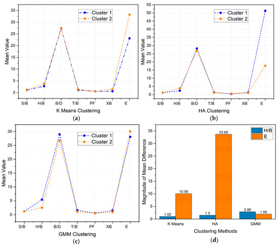
Figure 6.
Comparing mean difference by features and by clustering method: (a) K-means clusters; (b) HA clusters; (c) GMM clusters; (d) Comparison of all clustering methods.
Figure 6d shows that the modulus of elasticity (E) produced the highest magnitude of distinction between the two groups. It is more pronounced in HA, where the magnitude of difference is 33.66 than with K-means, which has a magnitude of difference of 10.06. This indicates that the modulus of elasticity (E) is a crucial feature that can provide a clear distinction between clusters. Therefore, this is a critical factor in predicting the cluster membership in new clusters. H/B was ranked second among all the features, with the value of the mean difference being the second highest.
2.3.5. Statistical Tests
The results of T statistics (two-way t-test) were used to determine whether there were significant differences between the means of the features of the two groups (see Table 4). The objective was to identify models with common attributes in terms of the overall statistical assessment. HA and K-means recorded the highest p-values outside the threshold alpha (α) value of 0.05, with each scoring 4/7 based on the number of features that were statistically significant. K-means and HA also had the highest measure of difference for t-statistics, 20.49 (E) and 12.22 (XB), respectively, which were also associated with the lowest p-values. This provided a basis for the evaluation of the two models. Table 4 shows all features of the two groups that were assessed.

Table 4.
T statistics of the features of the two groups based on clustering method.
2.4. Data Augmentation Using SMOGN
The synthetic minority oversampling technique for regression with Gaussian noise (SMOGN) addresses class imbalance by generating synthetic records by oversampling the minority class to balance the class distribution. It randomly produces new data samples through interpolation from the nearest neighborhood of minority class data [32]. The advantage of this technique is the generation of new and unique data points of the same class that are not duplicates. SMOGN was selected for its simplicity and effectiveness. Owing to the imbalanced nature of our clustered data, especially with reference to Cluster 1, data augmentation was implemented to improve the sample size and thus provide an adequate sample size for our machine learning exercise. Figure 7 and Figure 8 show scatter plots, feature distribution plots, and violin plots, respectively, which compare the real and augmented data obtained using the SMOGN. When assessing the quality of the generated data, the violin plots between the real and generated data should closely match in terms of the shape and spread. As can also be observed from the ensuing plots in Figure 9 and Figure 10, this condition is satisfied.

Figure 7.
(a) Scatter plot of real vs synthetic data points; (b) frequency distribution of H/B in KMC1 dataset.
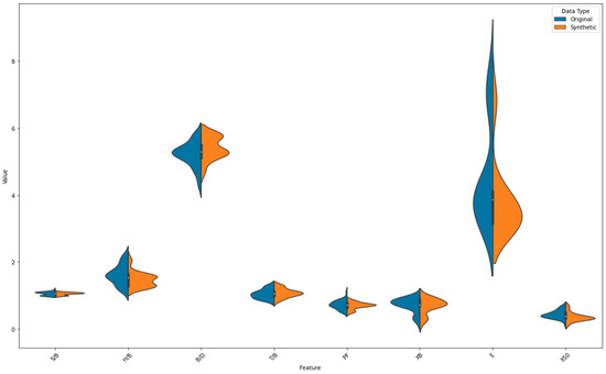
Figure 8.
Violin plot of original vs. synthetic for KMC1 dataset.
Below are the SMOGN generated data for HAC1.
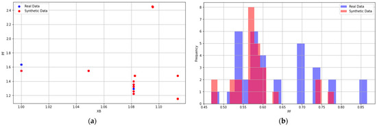
Figure 9.
(a) Scatter plot of real vs synthetic data points; (b) frequency distribution of PF in HAC1 dataset.
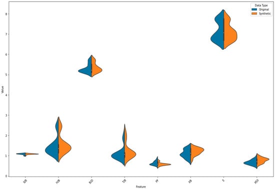
Figure 10.
Violin plot of HAC1 augmented data using SMOGN.
2.5. Data Processing for Machine Learning
A square root transformation was performed on the original data to handle the skewness and reduce the impact of outliers. This was also aimed at improving the data distribution to achieve normal distribution. As shown in Figure 11, the initial assessments noted that the square root transformation would most likely lead to better machine performance compared to the original data, as values that tended towards 0 were indicative of a better distribution.
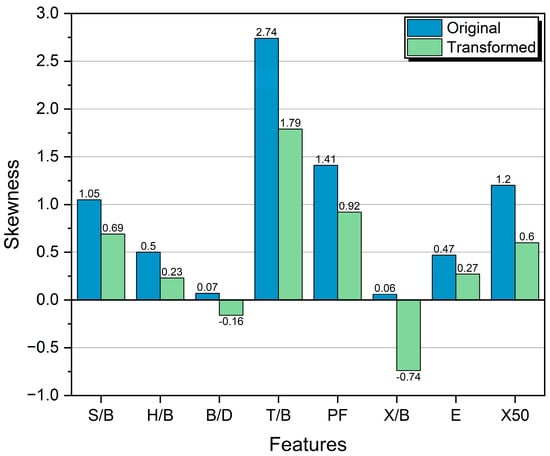
Figure 11.
Comparison of skewness—before and after square root transformation.
Table 5 presents the search spaces exposed to the search optimization algorithms. A small or limited search space was used to illustrate the impact of data augmentation using the SMOGN. A larger or expanded search space was used to determine the performance of different models over a large search space.

Table 5.
Search space configuration for selected hyperparameters.
The process of training the models is illustrated in Figure 12.
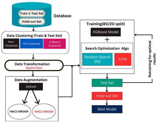
Figure 12.
Proposed framework used to predict the mean fragment size.
2.6. Evaluation Metrics
Two statistical measures, Mean Square Error (MSE) and coefficient of determination (R2), were employed as assessment metrics to evaluate the performance of the models. The MSE was used as the error criterion to determine the optimized hybrid models. R2 plays a crucial role in measuring model fitness, particularly in explaining variance in the data. By combining these two statistical measures, any misleading conclusions in model selection were avoided, ensuring a robust process that led to the selection of the model with the highest predictive power.
where
is the predicted value,
is the actual value,
is the mean of the actual values, and N the number of data points.
3. Results
3.1. Assessing the Impact of Clustering before SMOGN Application
The performances of the training and test sets were investigated to establish a baseline for assessing the impact of clustering; that is, the model performances on non-clustered and clustered datasets were compared to determine whether substantial benefits to the models accrued as a result of grouping.
3.1.1. Non-Clustered Data Set (Train and Test)
The transformed dataset with 97 blast points represents non-clustered data, principally set aside for training and testing. The objective of the analysis was to assess which predictive model between RS and ATPE would best leverage non-clustering. This marked the beginning of the model evaluation phase. 80% of this set was used for training and the remaining 20% was set aside for testing. Both the RS and ATPE were applied to 97 data points (77 for training and 20 for testing). Figure 13 shows line graphs depicting the performance of the trained models on the test set. It was apparent that ATPE demonstrated its superiority in predicting the mean fragment size from blasting operations, as it pertains to non-clustered datasets.
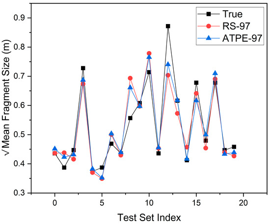
Figure 13.
Comparing the performance of RS-97 and ATPE-97.
Subsequently, the models were exposed to 13 new unseen blast data points in the holdout dataset. Table 6 lists the members of the hold-out set and their attributes.

Table 6.
Samples of the hold-out set.
As can be observed from the comparisons in Figure 14, ATPE-97 recorded considerably better prediction results in most instances and was thus consistent with its performance in the test set.
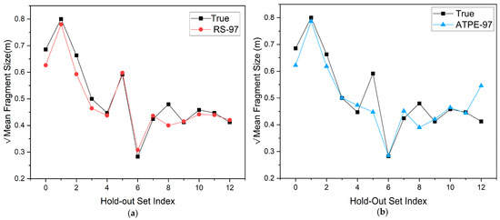
Figure 14.
Performance of RS-97 and ATPE-97 on the hold-out set. (a) RS-97 model, (b) ATPE-97 model.
3.1.2. Clustered Data Set (Train and Test)
Based on previous studies [15,16] that indicated clustering as a method for enhancing the performance and interpretability of machine learning models, clustering was first performed and applied to the training and test sets (97 blast points). Prior to the training, clustering was applied to the hold-out set. The 13 data points (hold-out set) were a subset of the entire database comprising 110 blast points; thus, for the purpose of identifying the cluster category for each of the new, unseen data, all the 110 blast samples were clustered. Consequently, HA using the Pearson Correlation Distance (PDC) with the Average Linkage Method proved effective because it resulted in a reasonable cluster size, that is, a data size that would be considered significant for any machine learning. HA produced 78 samples in Cluster 2 and 32 samples in Cluster 1. However, K-means produced 89 and 21 samples for Clusters 2 and 1, respectively. As presented in Table 7, the cluster membership of the hold-out set is based on the outcome of this process. The inherent groupings were identified as HAC1, HAC2, KMC1, and KMC2, with C1 and C2 representing Clusters 1 and 2, respectively. As indicated in Table 7, HAC2 had 10 blast samples and HAC1 had 3 blast samples. KMC2 had 11 blast sample points, whereas KMC1 had only 2 blast sample points.

Table 7.
Clustering members of the hold-out-set.
The following graphs depict the model performance results when exposed to the clustered datasets. The importance of these outcomes dictates the application of these models in real-world environments, where they can be used to estimate the mean fragment size of a muckpile with high accuracy.
3.1.3. Performance of Cluster 2 Models on New, Unseen Data
Cluster 2 had a significantly larger data size than Cluster 1; thus, to a substantial degree, it was more likely to provide relatively more reliable and stable performance. The hold-out set for Cluster 2 comprises 10 of the 13 members of the original hold-out set. Figure 15 shows a comparison of the results obtained after testing the models on the hold-out set. ATPE-HAC2 showed remarkable performance, registering minimal errors in predicting mean fragment size.
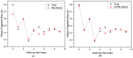
Figure 15.
Comparing performance of RS-HAC2 and ATPE-HAC2 on the hold-out set. (a) RS-HAC2 model. (b) ATPE-HAC2 model.
As shown in Figure 16, ATPE-KMC2 exhibited slightly better performance when gauged against the observed values in the hold-out set. While it achieved an R2 of 0.41, RS-KMC2 managed a lower R2 of 0.31. When evaluating the performance of these two predictive models against the true values, both generally exhibited high error rates, indicating substantial deviations between the actual and predicted values. This suggests that both models struggle to capture the underlying patterns in the data accurately. The differences between the predictions of the RS-KMC2 and ATPE-KMC2 models were smaller than those between the predictions of both models and the true values, suggesting an overall poor performance. This implies that both models may have captured similar aspects of the data, albeit insufficiently.
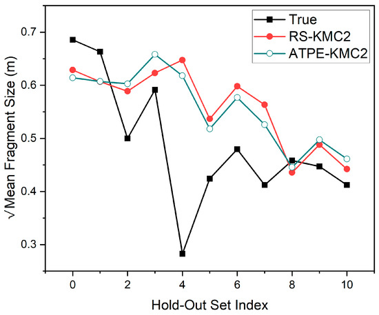
Figure 16.
Comparing the performance of RS and ATPE over KMC2 dataset.
3.1.4. Assessment of Clustering Impact on Cluster 2 Models
As previously mentioned, clustering is likely to improve the accuracy and robustness of the model. Therefore, this section evaluates whether the clustering is impactful. To ascertain this, the predicted values of the clustered models were examined and compared with their respective true values from the original hold-out set (13 data points). The main criterion was based on the search optimization algorithm used, i.e., RS or ATPE.
Bar plots were used to demonstrate alignment with the true values to easily identify the general performance and to determine overestimates and underestimates. The line of true fit illustrates a perfect prediction scenario, in which the predicted values match the actual values. The closer the proximity of a fit line to the line of true fit (y = x), the higher the prediction accuracy. As illustrated in Figure 17b, the line of fit for RS-97, with an R2 value of 0.93, is closer to the true fit line than that for RS-HAC2 (R2 = 0.89). In addition, the majority of the scattered plots are near the line of true fit for RS-97 compared to RS-HAC2, which are slightly spaced out. This implies that the RS-97 model is reliable and can be used to consistently reproduce more accurate mean fragment size values when Random Search is applied to the search space. The bar graph in Figure 17a presents a visualization of the general performance of the models. Good performance of the models was deduced, with only notable underestimates recorded for blasts with indices (0 and 5).
According to Figure 17d, the line of fit for ATPE-HAC2 with an R2 of 0.97 was closest to the true fit line, whereas that for ATPE-97 displayed a relatively large intersection angle with the true fit line, indicating a high dispersion between the predicted and actual values and had an R2 of 0.85. The scatter plots of the ATPE-HAC2 model were more compact and clustered around the true fit line, indicating that the model significantly captured the underlying pattern. In this case, clustering was proven impactful. A notable underestimation was observed for blast index 5.
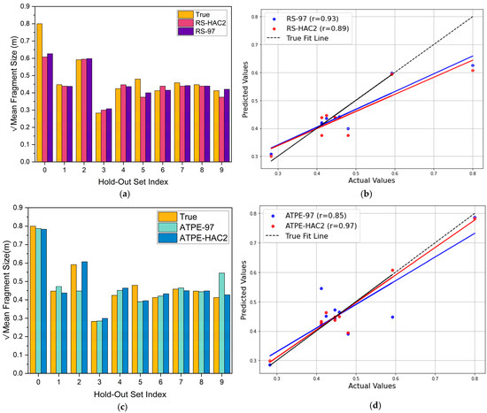
Figure 17.
Assessing clustering impact on HAC2 dataset. (a) Comparison of RS-97 and RS-HAC2 with True values. (b) Scatter plot comparing RS-97 and RS-HAC2. (c) Comparison of ATPE-97 and ATPE-HAC2 with True values. (d) Scatter plot comparing ATPE-97 and ATPE-HAC2.
As shown in Figure 18a,b, the assessment of K-means clustered data over a Random Search space reveals the superior performance of RS-97. It boasts a high R2 of 0.96 compared to that of RS-KMC2 with an R2 of 0.31. This means that it has a smaller intersection angle in comparison to the larger intersection angle of RS-KMC2, as well as a more compact cluster. This led to the conclusion that data clustering using K-means for Cluster 2 did not have a significant impact. It can be pointed out that there are a considerable number of underestimates and overestimates, with blast index 4 being the most pronounced. A similar inference was made for the search space over which the ATPE was deployed. As shown in Figure 18c, clustering using K-means did not improve the prediction quality. As can be observed, the line of fit for ATPE-97 was closer (r = 0.8) to the true fit line than that of ATPE-KMC2 (r = 0.41).
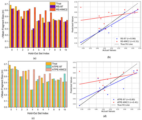
Figure 18.
Assessing the clustering impact on the KMC2 dataset. (a) Comparison of RS-97 and RS-KMC2 with True values. (b) Scatter plot comparing RS-97 and RS-KMC2. (c) Comparison of ATPE-97 and ATPE-KMC2 with True values. (d) Scatter plot comparing ATPE-97 and ATPE-KMC2.
3.2. Assessing the Impact of SMOGN on Cluster 1 Models Utilizing Limited Search Space
As stated earlier, clustering resulted in the following two clusters: Cluster 1 (C1) and Cluster 2 (C2). The consequence was C1 grouping, which had limited data compared to the data in C2. As noted for [33,34], blasting data are often challenging to acquire because of the infrequency of blasting in most operations. Consequently, it is difficult to assess the impact of clustering, particularly for imbalanced data. Thus, the synthetic minority oversampling technique for regression with Gaussian noise (SMOGN) was applied to the HAC1 and KMC1 models, which exhibited significant class imbalance. The main goal was to determine how data augmentation improved the generalization ability of the respective models. A total of 20 XGBoost–Random Search hybrid models were trained and tested with each model undergoing 5000 iterations. The best four models based on MSE and R squared were afterwards selected. The best model based on the clustering technique is represented by Model 4 in Figure 19 and Figure 20.
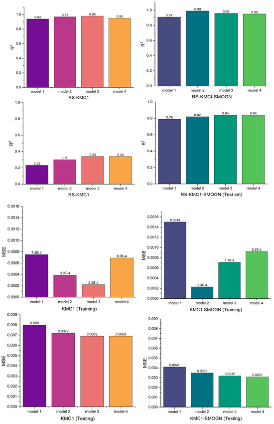
Figure 19.
Assessing SMOGN impact on KMC1 based on R2 and MSE over RS search space.
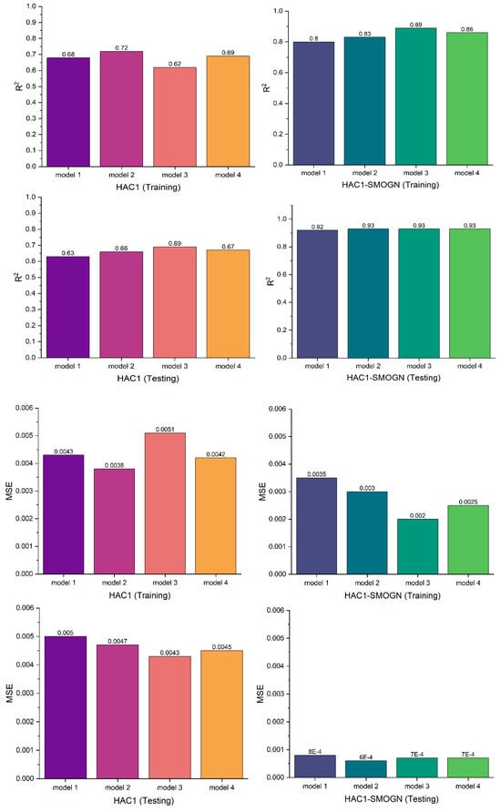
Figure 20.
Assessing SMOGN impact on HAC1 based on MSE and R Squared over RS search space.
Bar plots were used to compare the performance of the KMC1-SMOGN and KMC1 datasets within a limited search space.
It is evident from Figure 19 that the application of SMOGN can lead to better machine performance. High prediction accuracy was achieved during training, but dismal prediction results obtained during testing point to overfitting. Model 4 for KMC1 and Model 4 for KMC1-SMOGN were the best among the selected models. KMC1-SMOGN exhibited an increase of approximately 47% in R2. This improvement is significant in machine learning. The most likely explanation for the poor performance of KMC1 is insufficient data, which makes it difficult for the model to comprehend the true underlying patterns that generalize well to new data.
KMC1 exhibits an overfitting tendency. However, while KMC1-SMOGN did not perform as well as KMC1 during training, it maintained lower MSE values, indicating better performance in avoiding overfitting (see Model 1). The SMOGN-augmented data demonstrated that the model did not overlearn the training data or capture noise, resulting in improved generalization capabilities.
As shown in Figure 20, when evaluating the impact of data augmentation on HAC1, although a similar trend was expected, the HAC1 models exhibited slightly peculiar behavior. The unaugmented models (HAC1) demonstrated less overfitting than the KMC1 models. A review of the MSE results is consistent with the results of R2. As shown in the same figure, the best overall HAC1-SMOGN model showed improved performance on the training set and further demonstrated stable performance, achieving an R2 of 0.93. This model also resulted in the most significant differences in reducing the objective function, that is, MSE minimization. It achieved R2/MSE values of 0.86/0.0025 during training and 0.93/0.0007 during testing. The best HAC1 performance for R2/MSE was 0.69/0.0042 during the training and 0.67/0.0045 during the testing.
Table 8 presents the performance and associated hyperparameters of the models used to evaluate the impact of the data augmentation.

Table 8.
Summary of the associated hyperparameters based on RS and limited search space.
Figure 20 shows the results of assessing the HAC1 and HAC1-SMOGN models.
By achieving the lowest MSE and highest R2, the KMC1-SMOGN and HAC1-SMOGN models successfully demonstrated the efficacy of applying SMOGN to improve the model performance.
3.3. Assessing the Impact of SMOGN and Influence of Search Space Configuration on Cluster 1 Models
The best-performing models were exposed to both the test set and hold-out set to assess their performance. The best overall model, ATPE-HAC1-SMOGN, over an expanded search space demonstrated satisfactory ability to generalize new, unseen data. Figure 21 presents an overview of its performance on the hold-out set. The effects of the selected search space were reviewed to determine the performance of the models. As shown in the figure, the search space range played a critical role. As illustrated in Figure 21a,c, the model performed better in the expanded search space than in the limited search space. In both cases, the higher number of ‘n_estimators’ was perhaps indicative of the greater potential to capture complex patterns. Deeper trees, as opposed to trees in a limited space, may allow detailed feature interactions. The combination of a higher learning rate and higher number of trees may have led to better convergence. The log-uniform distributions of the learning rate used in the expanded search space may have allowed the exploration of smaller values that are critical for fine-tuning. It appears from the analysis of Figure 21 that although both models show strong performance, the models in the larger search space led to more robust models with better generalization abilities. To determine that this was indeed the case, as presented in Figure 21b,d, these models were exposed to the hold-out set in Cluster 1, i.e., three blasts for HAC1 and two blasts for KMC1. Overall, ATPE-HAC1-SMOGN has emerged as the model with the highest performance over the expanded search space. The performances of the other models were equally impressive. In general, no visual pickouts indicated extreme overestimation or underestimation. In addition, the performance of ATPE-KMC1-SMOGN was assessed within the expanded search space. Interestingly, Random Search (RS) over the expanded space not only matched Mr12 (0.53), but also outperformed ATPE-KMC1-SMOGN in the limited search space for Ru7 (0.49 compared to 0.51 against a true value of 0.8). This suggests that even though RS is generally regarded as a less powerful search optimization algorithm, it can surpass more advanced algorithms, such as ATPE, depending on the characteristics of the search space.
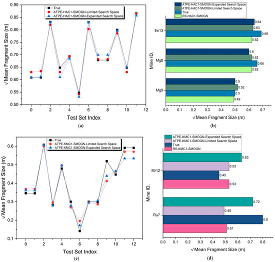
Figure 21.
Comparing model performances based on search space configuration and performance on the hold-out set. (a) ATPE-HAC1-SMOGN performance comparison on Limited & Expanded Search Space. (b) HAC1-SMOGN models’ performance on the hold-out set. (c) ATPE-KMC1-SMOGN performance comparison on Limited & Expanded Search Space. (d) KMC1-SMOGN models’ performance on the hold-out set.
Table 9 summarizes the associated models and their performance.

Table 9.
Summarized results of hyperparameters and respective model performances.
4. Discussion
In this study, when assessing the performance of different models, we were able to draw conclusions that highlight the advantages of the methods employed. ATPE, as a search space optimization algorithm, exhibited robust performance when compared to the Random Search algorithm. Models using ATPE on both clustered and non-clustered data showed that they were superior to RS. Although RS is a simple method, it demonstrated that it can also accurately predict the mean fragment size. The superior performance of ATPE might be attributed to its efficiency owing to its sequential optimization, as opposed to RS, where the optimization strategy can be termed ‘non-adaptive.’
The nature of the algorithm used for search space optimization determines the time that the model trains before convergence. Owing to its simplicity, RS, given a similar search space and the same number of iterations during training, was found to be computationally faster than ATPE.
As presented in Table 9, the two investigated search spaces generated two distinct probability density functions (PDFs). One is associated with smaller hyperparameter values and a larger search space results in large numbers (for example, n_estimators) and the use of comparatively higher learning rate values. A larger search space implies that exploration and exploitation would span a wider area; consequently, the probability of obtaining a global solution is enhanced. Although large search spaces are often associated with overfitting tendencies and while most models displayed some overfitting tendencies, a model such as ATPE-HAC1-SMOGN demonstrated robust performance, proving its reliability.
The superior predictive performance due to hyperparameter tuning is another highlight of this study. The XGBoost as the core model proved to be robust most likely due to the fact that it had a regularization term for handling model complexity and for managing overfitting. The hyperparameters for the mean fragment size regression model, that is, the learning rate, maximum depth, n_estimators, gamma, subsample, colsample_bytree, and min_child_weight, were also crucial in balancing the capacity of the model to learn complex patterns and generalize well to unseen data, with the aim of minimizing both overfitting and underfitting. For example, the best models were found to use lower gamma values (e.g., 0.0004 for ATPE-HAC1-SMOGN). Such low values may have allowed the model to create more splits, thereby allowing it to capture more detailed patterns.
When evaluating the impact of the clustering techniques, it was evident that hierarchical clustering was highly effective owing to its outstanding performance over K-means clustering. The HA model outputs were closer to the real values than those of the K-means. This may be largely attributed to the powerful nature of HA, which can capture structures more effectively than K-means, particularly if the data contain clusters of complex and non-complex shapes. Moreover, it is possible that the merge or split points, which are critical factors used in creating the cluster, were well chosen, resulting in high-quality clusters. K-means is more suited for handling large datasets, whereas HA, because of its higher computational complexity, is more suited for small-to medium-sized datasets, as is the case with our dataset. K-means is highly sensitive to the initial placement of centroids. Suboptimal clustering results and convergence to local minima in K-means clustering are often associated with poor initialization. The selection of the two clusters was based on domain knowledge, which may have led to the underperformance of the K-means clustering. The elbow and silhouette analysis recommended an optimal K of seven, although for the purposes of our machine learning, the dataset based on the clusters would be highly limited in terms of size. This means that the resulting cluster quality was moderate or nonideal. This points to the debate that machine learning engineers face, that is, balancing domain knowledge and statistical recommendations. In addition, the Euclidean distance metric may not be an ideal metric for measuring the similarity between data points.
This study also demonstrated the significance of data augmentation. The application of SMOGN to Cluster 1 of both K-means and HA showed that the data augmentation technique enhanced the performance of the models by reducing their tendency to overfit. Although the other models performed well, HAC1-SMOGN performed the best, with an MSE of 0.00023 and an R2 of 0.98. Assessment of the training, testing, and performance on the hold-out set showed that the model displayed great learning ability and was able to generalize well, not only on the test data, but also on the new, unseen data. This confirms that SMOGN is robust and continues to be a standard benchmark for handling challenges associated with imbalanced data in regression problems.
5. Conclusions
Our investigation of the application of machine learning via regression to predict the mean fragment size in rock blasting operations yielded valuable insights into search optimization for hyperparameter tuning and the significance of clustering and also addressed the issue of data imbalance through data augmentation.
The following can be concluded from this research:
- ATPE outperformed Random Search in search space optimization, resulting in more accurate predictions of the mean fragment size. However, ATPE models were slower to train than Random Search, which were faster due to their simplistic nature.
- Hierarchical clustering (HA) is more effective than K-means clustering in capturing complex data structures, leading to better model performance.
- XGBoost models tuned using ATPE showed strong performance owing to well-balanced hyperparameter tuning, which helped manage model complexity and generalization.
- The application of SMOGN significantly enhanced model performance by reducing overfitting, particularly in HA clusters.
- The research demonstrated that models in a larger search space generally achieved better performance, suggesting a greater likelihood of finding global solutions. However, it should be noted that large probability density functions increase the risk of overfitting unless robust models are used.
In conclusion, the small sample size was a limitation of this study. A large dataset with a good distribution would have yielded adequate data sample points, particularly in the clustered hold-out set. Other search optimization algorithms (SOAs), such as evolutionary algorithms, should be evaluated, especially over an expanded search space, to establish the performance and model training duration. Only one data-augmentation technique was used. In the future, other methods, such as adaptive synthetic sampling (ADASYN), bootstrapping, or variational autoencoders (VAEs), will be developed.
Author Contributions
Conceptualization, I.K.; Methodology, I.K. and A.H.; Software, I.K.; Validation, I.K. and T.S.; data curation, I.K., and A.H.; writing—original draft preparation, I.K.; writing—review and editing, T.S. and H.S.; visualization I.K.; supervision, T.S. and H.S. All authors have read and agreed to the published version of the manuscript.
Funding
The research work is part of a doctoral program supported by JICA.
Institutional Review Board Statement
Not applicable.
Informed Consent Statement
Not applicable.
Data Availability Statement
The data source used is cited, and all the data produced are reported in the manuscript.
Acknowledgments
We acknowledge JICA’s invaluable support, without which this research would not have been possible.
Conflicts of Interest
The authors declare no conflicts of interest.
Appendix A. Original Data (Hudaverdi et al. [14])

Table A1.
Parameters.
Table A1.
Parameters.
| Blast No. | Blast ID. | S/B | H/B | B/D | T/B | PF (kg/m3) | XB (m) | E (GPa) | X50 (m) |
|---|---|---|---|---|---|---|---|---|---|
| 1 | En1 | 1.24 | 1.33 | 27.27 | 0.78 | 0.48 | 0.58 | 60 | 0.37 |
| 2 | En2 | 1.24 | 1.33 | 27.27 | 0.78 | 0.48 | 0.58 | 60 | 0.37 |
| 3 | En3 | 1.24 | 1.33 | 27.27 | 0.78 | 0.48 | 1.08 | 60 | 0.33 |
| 4 | En4 | 1.24 | 1.33 | 27.27 | 0.78 | 0.48 | 1.11 | 60 | 0.42 |
| 5 | En5 | 1.24 | 1.33 | 27.27 | 0.78 | 0.48 | 1.08 | 60 | 0.46 |
| 6 | En6 | 1.24 | 1.33 | 27.27 | 1.17 | 0.27 | 1.08 | 60 | 0.37 |
| 7 | En7 | 1.24 | 1.33 | 27.27 | 1.06 | 0.33 | 1.08 | 60 | 0.64 |
| 8 | En8 | 1.24 | 1.33 | 27.27 | 0.91 | 0.41 | 1.11 | 60 | 0.42 |
| 9 | En9 | 1.24 | 1.33 | 27.27 | 0.91 | 0.41 | 1.11 | 60 | 0.26 |
| 10 | En10 | 1.24 | 1.33 | 27.27 | 0.99 | 0.36 | 1.08 | 60 | 0.42 |
| 11 | En11 | 1.24 | 1.33 | 27.27 | 1.06 | 0.33 | 1.11 | 60 | 0.31 |
| 12 | En12 | 1.24 | 1.33 | 27.27 | 1.06 | 0.33 | 1.11 | 60 | 0.38 |
| 13 | Rc1 | 1.17 | 1.5 | 26.2 | 1.08 | 0.33 | 0.68 | 45 | 0.46 |
| 14 | Rc2 | 1.17 | 1.5 | 26.2 | 1.12 | 0.3 | 0.68 | 45 | 0.48 |
| 15 | Rc3 | 1.17 | 1.58 | 26.2 | 1.22 | 0.28 | 0.68 | 45 | 0.48 |
| 16 | Rc4 | 1.17 | 1.96 | 26.2 | 1.3 | 0.34 | 1.56 | 45 | 0.75 |
| 17 | Rc5 | 1.17 | 1.75 | 26.2 | 1.31 | 0.29 | 1.56 | 45 | 0.96 |
| 18 | Rc6 | 1.17 | 1.75 | 26.2 | 1.16 | 0.36 | 1.56 | 45 | 0.76 |
| 19 | Rc7 | 1.17 | 1.67 | 26.2 | 1.22 | 0.31 | 1.8 | 45 | 0.53 |
| 20 | Rc8 | 1.17 | 1.83 | 26.2 | 1.34 | 0.3 | 1.8 | 45 | 0.56 |
| 21 | Rc9 | 1.17 | 1.83 | 26.2 | 1.29 | 0.32 | 1.8 | 45 | 0.74 |
| 22 | Rc10 | 1.17 | 1.83 | 26.2 | 1.23 | 0.35 | 1.8 | 45 | 0.44 |
| 23 | Mg1 | 1 | 2.67 | 27.27 | 0.89 | 0.75 | 0.83 | 50 | 0.23 |
| 24 | Mg2 | 1 | 2.67 | 27.27 | 0.89 | 0.75 | 0.78 | 50 | 0.25 |
| 25 | Mg3 | 1 | 2.4 | 30.3 | 0.8 | 0.61 | 1.02 | 50 | 0.27 |
| 26 | Mg4 | 1 | 2.4 | 30.3 | 0.8 | 0.61 | 0.75 | 50 | 0.3 |
| 27 | Mg5 | 1.1 | 2.4 | 30.3 | 0.8 | 0.55 | 1.18 | 50 | 0.38 |
| 28 | Mg6 | 1.1 | 2.4 | 30.3 | 0.8 | 0.55 | 1.24 | 50 | 0.37 |
| 29 | Mg7 | 1.1 | 2.4 | 30.3 | 0.8 | 0.55 | 1.33 | 50 | 0.38 |
| 30 | Ru1 | 1.13 | 5 | 39.47 | 1.93 | 0.31 | 2 | 45 | 0.64 |
| 31 | Ru2 | 1.2 | 6 | 32.89 | 3.67 | 0.3 | 2 | 45 | 0.54 |
| 32 | Ru3 | 1.2 | 6 | 32.89 | 3.7 | 0.3 | 2 | 45 | 0.51 |
| 33 | Ru4 | 1.2 | 6 | 32.89 | 4.67 | 0.22 | 2 | 45 | 0.64 |
| 34 | Ru5 | 1.2 | 6 | 32.89 | 3.11 | 0.35 | 2 | 45 | 0.54 |
| 35 | Ru6 | 1.2 | 6 | 32.89 | 3.22 | 0.34 | 2 | 45 | 0.69 |
| 36 | Mr1 | 1.2 | 6 | 32.89 | 0.8 | 0.49 | 1.67 | 32 | 0.17 |
| 37 | Mr2 | 1.2 | 6 | 32.89 | 0.8 | 0.51 | 1.67 | 32 | 0.17 |
| 38 | Mr3 | 1.2 | 6 | 32.89 | 0.8 | 0.49 | 1.67 | 32 | 0.13 |
| 39 | Mr4 | 1.2 | 6 | 32.89 | 0.8 | 0.52 | 1.67 | 32 | 0.17 |
| 40 | Mr5 | 1.2 | 6 | 32.89 | 0.8 | 0.42 | 1.67 | 32 | 0.13 |
| 41 | Mr6 | 1.4 | 6 | 32.89 | 0.8 | 0.36 | 1.67 | 32 | 0.15 |
| 42 | Mr7 | 1.2 | 6 | 32.89 | 0.6 | 0.56 | 1.03 | 32 | 0.18 |
| 43 | Mr8 | 1.4 | 6 | 32.89 | 0.6 | 0.3 | 1.03 | 32 | 0.19 |
| 44 | Mr9 | 1.4 | 6 | 32.89 | 0.6 | 0.35 | 1.03 | 32 | 0.16 |
| 45 | Mr10 | 1.16 | 5 | 39.47 | 0.5 | 0.39 | 1.03 | 32 | 0.17 |
| 46 | Mr11 | 1.16 | 5 | 39.47 | 0.5 | 0.32 | 1.03 | 32 | 0.21 |
| 47 | Db1 | 1.25 | 3.5 | 20 | 1.75 | 0.73 | 1 | 9.57 | 0.44 |
| 48 | Db2 | 1.25 | 5.1 | 20 | 1.75 | 0.7 | 1 | 9.57 | 0.76 |
| 49 | Db3 | 1.38 | 3 | 20 | 1.75 | 0.62 | 1 | 9.57 | 0.35 |
| 50 | Db4 | 1.5 | 5.5 | 20 | 1.75 | 0.56 | 1 | 9.57 | 0.55 |
| 51 | Db5 | 1.75 | 4.75 | 20 | 1.75 | 0.39 | 1 | 9.57 | 0.35 |
| 52 | Db6 | 1.25 | 4.75 | 20 | 1.75 | 0.33 | 1 | 9.57 | 0.23 |
| 53 | Db7 | 1.25 | 5 | 20 | 1.75 | 0.44 | 1 | 9.57 | 0.4 |
| 54 | Db8 | 1.2 | 2.4 | 25 | 1.4 | 0.28 | 0.5 | 9.57 | 0.35 |
| 55 | Db9 | 1.4 | 3.2 | 25 | 1.4 | 0.31 | 0.5 | 9.57 | 0.29 |
| 56 | Mi1 | 1 | 2.5 | 22.22 | 1.69 | 0.71 | 0.17 | 10 | 0.1 |
| 57 | Mi2 | 1 | 1.67 | 33.33 | 0.72 | 0.46 | 0.1 | 10 | 0.09 |
| 58 | Mi3 | 1 | 1.67 | 33.33 | 1.25 | 0.27 | 0.1 | 10 | 0.09 |
| 59 | Mi4 | 1 | 1.67 | 33.33 | 0.7 | 0.47 | 0.1 | 10 | 0.08 |
| 60 | Mi5 | 1 | 1.67 | 33.33 | 1.28 | 0.26 | 0.1 | 10 | 0.1 |
| 61 | Mi6 | 1 | 2.5 | 22.22 | 1.69 | 0.71 | 0.02 | 10 | 0.02 |
| 62 | Sm1 | 1.25 | 2.5 | 28.57 | 0.83 | 0.42 | 0.5 | 13.25 | 0.15 |
| 63 | Sm2 | 1.25 | 2.5 | 28.57 | 0.83 | 0.42 | 0.5 | 13.25 | 0.19 |
| 64 | Sm3 | 1.25 | 2.5 | 28.57 | 0.83 | 0.42 | 0.5 | 13.25 | 0.23 |
| 65 | Sm4 | 1.25 | 2.5 | 28.57 | 0.83 | 0.42 | 1.5 | 13.25 | 0.22 |
| 66 | Sm5 | 1.25 | 2.5 | 28.57 | 0.83 | 0.42 | 1.5 | 13.25 | 0.24 |
| 67 | Sm6 | 1.25 | 2.5 | 28.57 | 0.83 | 0.42 | 1.5 | 13.25 | 0.26 |
| 68 | Sm7 | 1.25 | 2.5 | 28.57 | 0.83 | 0.42 | 1.5 | 13.25 | 0.28 |
| 69 | Ad1 | 1.2 | 4.4 | 28.09 | 1.2 | 0.58 | 0.77 | 16.9 | 0.15 |
| 70 | Ad2 | 1.2 | 4.8 | 28.09 | 1.2 | 0.66 | 0.56 | 16.9 | 0.17 |
| 71 | Ad3 | 1.2 | 4.8 | 28.09 | 1.2 | 0.72 | 0.29 | 16.9 | 0.14 |
| 72 | Ad4 | 1.2 | 4 | 28.09 | 1.6 | 0.49 | 0.81 | 16.9 | 0.16 |
| 73 | Ad5 | 1.14 | 6.82 | 24.72 | 1.36 | 0.84 | 1.43 | 16.9 | 0.21 |
| 74 | Ad6 | 1.14 | 6.36 | 24.72 | 1.36 | 0.82 | 1.77 | 16.9 | 0.21 |
| 75 | Ad7 | 1.25 | 3.5 | 22.47 | 1.25 | 0.75 | 1.03 | 16.9 | 0.15 |
| 76 | Ad8 | 1.25 | 3.25 | 22.47 | 1.25 | 0.71 | 0.83 | 16.9 | 0.19 |
| 77 | Ad9 | 1.25 | 3.5 | 22.47 | 1.25 | 0.76 | 1.68 | 16.9 | 0.18 |
| 78 | Ad10 | 1.25 | 3.5 | 22.47 | 1.25 | 0.76 | 1.24 | 16.9 | 0.15 |
| 79 | Ad11 | 1.14 | 3.18 | 24.72 | 1.14 | 0.69 | 0.67 | 16.9 | 0.14 |
| 80 | Ad12 | 1.14 | 3.18 | 24.72 | 1.14 | 0.69 | 2.01 | 16.9 | 0.2 |
| 81 | Ad13 | 1.12 | 2.8 | 28.09 | 1 | 0.54 | 0.96 | 16.9 | 0.15 |
| 82 | Ad14 | 1 | 2.4 | 28.09 | 1 | 0.56 | 0.83 | 16.9 | 0.14 |
| 83 | Ad15 | 1.1 | 3.75 | 21.74 | 1 | 1.02 | 1.64 | 16.9 | 0.15 |
| 84 | Ad16 | 1.1 | 3.5 | 22.47 | 1.25 | 0.86 | 2.35 | 16.9 | 0.15 |
| 85 | Ad17 | 1.25 | 3.75 | 17.98 | 1.56 | 1.24 | 1.53 | 16.9 | 0.19 |
| 86 | Ad18 | 1 | 4 | 18.42 | 1.71 | 1.26 | 0.73 | 16.9 | 0.15 |
| 87 | Ad19 | 1 | 4 | 18.42 | 1.71 | 1.26 | 1.47 | 16.9 | 0.17 |
| 88 | Ad20 | 1.14 | 4 | 18.42 | 1.71 | 1.1 | 1.19 | 16.9 | 0.19 |
| 89 | Ad21 | 1.11 | 4.44 | 18.95 | 1.67 | 1.25 | 1.71 | 16.9 | 0.22 |
| 90 | Ad22 | 1.28 | 3.61 | 18.95 | 1.67 | 0.89 | 0.56 | 16.9 | 0.2 |
| 91 | Oz1 | 1 | 2.83 | 33.71 | 1 | 0.48 | 0.45 | 15 | 0.27 |
| 92 | Oz2 | 1.2 | 2.4 | 28.09 | 1 | 0.53 | 0.86 | 15 | 0.14 |
| 93 | Oz3 | 1.2 | 2.4 | 28.09 | 1 | 0.53 | 0.44 | 15 | 0.14 |
| 94 | Oz4 | 1.25 | 4.5 | 22.47 | 1.5 | 0.76 | 0.66 | 15 | 0.2 |
| 95 | Oz5 | 1.11 | 3.33 | 30.34 | 1.11 | 0.47 | 0.47 | 15 | 0.17 |
| 96 | Oz6 | 1.2 | 3.2 | 28.09 | 1.2 | 0.48 | 1.11 | 15 | 0.3 |
| 97 | Oz7 | 1.2 | 2.4 | 28.09 | 1 | 0.53 | 0.88 | 15 | 0.12 |
| 98 | En13 | 1.24 | 1.33 | 27.27 | 0.78 | 0.48 | 1.11 | 60 | 0.47 |
| 99 | Ru7 | 1.13 | 5 | 39.47 | 3.11 | 0.31 | 2 | 45 | 0.64 |
| 100 | Mg8 | 1.1 | 2.4 | 30.3 | 0.8 | 0.55 | 1.23 | 50 | 0.44 |
| 101 | Mg9 | 1 | 2.67 | 27.27 | 0.89 | 0.75 | 0.77 | 50 | 0.25 |
| 102 | Mr12 | 1.25 | 6.25 | 31.58 | 0.63 | 0.48 | 1.03 | 32 | 0.2 |
| 103 | Db10 | 1.15 | 4.35 | 20 | 1.75 | 0.89 | 1 | 9.57 | 0.35 |
| 104 | Mi7 | 1 | 1.67 | 33.33 | 0.7 | 0.47 | 0.09 | 10 | 0.08 |
| 105 | Sm8 | 1.25 | 2.5 | 28.57 | 0.83 | 0.42 | 0.5 | 13.25 | 0.18 |
| 106 | Oz8 | 1.2 | 2.4 | 28.09 | 1 | 0.53 | 0.82 | 15 | 0.23 |
| 107 | Oz9 | 1.11 | 3.33 | 30.34 | 1.11 | 0.47 | 0.54 | 15 | 0.17 |
| 108 | Ad23 | 1.11 | 4.44 | 18.95 | 1.67 | 1.25 | 1.63 | 16.9 | 0.21 |
| 109 | Ad24 | 1.28 | 3.61 | 18.95 | 1.67 | 0.89 | 0.61 | 16.9 | 0.2 |
| 110 | Ad25 | 1.2 | 2.8 | 28.09 | 1 | 0.5 | 1.49 | 16.9 | 0.17 |
References
- Roy, M.P.; Paswan, R.K.; Sarim, M.D.; Kumar, S.U.R.A.J.; Jha, R.; Singh, P.K. Rock Fragmentation by Blasting—A Review. 2016. Available online: https://www.researchgate.net/publication/317031336 (accessed on 27 June 2024).
- Zhang, Z.-X.; Hou, D.-F.; Guo, Z.; He, Z.; Zhang, Q. Experimental study of surface constraint effect on rock fragmentation by blasting. Int. J. Rock Mech. Min. Sci. Géoméch. Abstr. 2020, 128, 104278. [Google Scholar] [CrossRef]
- Zhang, Z.-X.; Sanchidrián, J.A.; Ouchterlony, F.; Luukkanen, S. Reduction of Fragment Size from Mining to Mineral Processing: A Review. Rock Mech. Rock Eng. 2022, 56, 747–778. [Google Scholar] [CrossRef]
- Armaghani, D.J. Rock Fragmentation Prediction through a New Hybrid Model Based on Imperial Competitive Algorithm and Neural Network. Smart Constr. Res. 2018, 2, 1–12. [Google Scholar] [CrossRef]
- Dumakor-Dupey, N.K.; Arya, S.; Jha, A. Advances in blast-induced impact prediction—A review of machine learning applications. Minerals 2021, 11, 601. [Google Scholar] [CrossRef]
- Bahrami, A.; Monjezi, M.; Goshtasbi, K.; Ghazvinian, A. Prediction of rock fragmentation due to blasting using artificial neural network. Eng. Comput. 2010, 27, 177–181. [Google Scholar] [CrossRef]
- Shi, X.Z.; Zhou, J.; Wu, B.B.; Huang, D.; Wei, W. Support vector machines approach to mean particle size of rock fragmentation due to bench blasting prediction. Trans. Nonferrous Met. Soc. China 2012, 22, 432–441. [Google Scholar] [CrossRef]
- Shi, X.-Z.; Zhou, J.; Wu, B.-B.; Huang, D.; Wei, W. Rock Fragmentation Size Distribution Prediction and Blasting Parameter Optimization Based on the Muck-Pile Model. Min. Metall. Explor. 2021, 38, 1071–1080. [Google Scholar] [CrossRef]
- Nabavi, Z.; Mirzehi, M.; Dehghani, H.; Ashtari, P. A Hybrid Model for Back-Break Prediction using XGBoost Machine learning and Metaheuristic Algorithms in Chadormalu Iron Mine. J. Min. Environ. 2023, 14, 689–712. [Google Scholar] [CrossRef]
- Zhang, X.; Nguyen, H.; Bui, X.N.; Tran, Q.H.; Nguyen, D.A.; Bui, D.T.; Moayedi, H. Novel Soft Computing Model for Predicting Blast-Induced Ground Vibration in Open-Pit Mines Based on Particle Swarm Optimization and XGBoost. Nat. Resour. Res. 2020, 29, 711–721. [Google Scholar] [CrossRef]
- Amoako, R.; Jha, A.; Zhong, S. Rock Fragmentation Prediction Using an Artificial Neural Network and Support Vector Regression Hybrid Approach. Mining 2022, 2, 233–247. [Google Scholar] [CrossRef]
- Xie, C.; Nguyen, H.; Bui, X.-N.; Choi, Y.; Zhou, J.; Nguyen-Trang, T. Predicting rock size distribution in mine blasting using various novel soft computing models based on meta-heuristics and machine learning algorithms. Geosci. Front. 2021, 12, 101108. [Google Scholar] [CrossRef]
- Jia, Z.; Song, Z.; Fan, J.; Jiang, J. Prediction of Blasting Fragmentation Based on GWO-ELM. Shock. Vib. 2022, 2022, 7385456. [Google Scholar] [CrossRef]
- Hudaverdi, T.; Kulatilake, P.H.S.W.; Kuzu, C. Prediction of blast fragmentation using multivariate analysis procedures. Int. J. Numer. Anal. Methods Géoméch. 2010, 35, 1318–1333. [Google Scholar] [CrossRef]
- Nguyen, H.; Bui, X.N.; Tran, Q.H.; Mai, N.L. A new soft computing model for estimating and controlling blast-produced ground vibration based on Hierarchical K-means clustering and Cubist algorithms. Appl. Soft Comput. 2019, 77, 376–386. [Google Scholar] [CrossRef]
- Sheykhi, H.; Bagherpour, R.; Ghasemi, E.; Kalhori, H. Forecasting ground vibration due to rock blasting: A hybrid intelligent approach using support vector regression and fuzzy C-means clustering. Eng. Comput. 2017, 34, 357–365. [Google Scholar] [CrossRef]
- Singh, N.D.; Dhall, A. Clustering and Learning from Imbalanced Data. 2018. Available online: http://arxiv.org/abs/1811.00972 (accessed on 7 July 2024).
- Yilmaz, O. Rock factor prediction in the Kuz–Ram model and burden estimation by mean fragment size. Geomech. Energy Environ. 2023, 33, 100415. [Google Scholar] [CrossRef]
- Ouchterlony, F.; Niklasson, B.; Abrahamsson, S. Fragmentation Monitoring of Production Blasts at MRICA. 1990. Available online: https://ltu.diva-portal.org/smash/get/diva2:1000771/FULLTEXT01.pdf (accessed on 3 July 2024).
- Chen, T.; Guestrin, C. XGBoost: A scalable tree boosting system. In Proceedings of the ACM SIGKDD International Conference on Knowledge Discovery and Data Mining, San Francisco, CA, USA, 13–17 August 2016; pp. 785–794. [Google Scholar] [CrossRef]
- Ali, Z.A.; Abduljabbar, Z.H.; Tahir, H.A.; Sallow, A.B.; Almufti, S.M. eXtreme Gradient Boosting Algorithm with Machine Learning: A Review. Acad. J. Nawroz Univ. 2023, 12, 320–334. [Google Scholar] [CrossRef]
- Cai, R.; Xie, S.; Wang, B.; Yang, R.; Xu, D.; He, Y. Wind speed forecasting based on extreme gradient boosting. IEEE Access 2020, 8, 175063–175069. [Google Scholar] [CrossRef]
- Shahani, N.M.; Zheng, X.; Liu, C.; Hassan, F.U.; Li, P. Developing an XGBoost Regression Model for Predicting Young’s Modulus of Intact Sedimentary Rocks for the Stability of Surface and Subsurface Structures. Front. Earth Sci. 2021, 9, 761990. [Google Scholar] [CrossRef]
- Rong, G.; Li, K.; Su, Y.; Tong, Z.; Liu, X.; Zhang, J.; Zhang, Y.; Li, T. Comparison of tree-structured parzen estimator optimization in three typical neural network models for landslide susceptibility assessment. Remote Sens. 2021, 13, 4694. [Google Scholar] [CrossRef]
- Bergstra, J.; Bengio, Y. Random Search for Hyper-Parameter Optimization Yoshua Bengio. 2012. Available online: http://scikit-learn.sourceforge.net (accessed on 20 May 2024).
- Watanabe, S. Tree-Structured Parzen Estimator: Understanding Its Algorithm Components and Their Roles for Better Empirical Performance. 2023. Available online: http://arxiv.org/abs/2304.11127 (accessed on 5 June 2024).
- Bergstra, J.; Bardenet, R.; Bengio, Y.; Kégl, B. Algorithms for Hyper-Parameter Optimization. In Proceedings of the Advances in Neural Information Processing Systems, Granada, Spain, 12–15 December 2011. [Google Scholar]
- Wen, L.; Ye, X.; Gao, L. A new automatic machine learning based hyperparameter optimization for workpiece quality prediction. Meas. Control 2020, 53, 1088–1098. [Google Scholar] [CrossRef]
- Effect of Different Distance Measures in Result of Cluster Analysis. Available online: www.aalto.fi (accessed on 7 July 2024).
- Pitafi, S.; Anwar, T.; Sharif, Z. A Taxonomy of Machine Learning Clustering Algorithms, Challenges, and Future Realms. Appl. Sci. 2023, 13, 3529. [Google Scholar] [CrossRef]
- Makwana, P.; Kodinariya, T.M.; Makwana, P.R. Review on Determining of Cluster in K-means Clustering Review on determining number of Cluster in K-Means Clustering. Int. J. Adv. Res. Comput. Sci. Manag. Stud. 2013, 1, 90–95. Available online: https://www.researchgate.net/publication/313554124 (accessed on 11 June 2024).
- Branco, P.; Torgo, L.; Ribeiro, R.P. SMOGN: A Pre-Processing Approach for Imbalanced Regression. 2017. Available online: https://www.researchgate.net/publication/319906917 (accessed on 21 June 2024).
- Krop, I.; Takahashi, Y.; Sasaoka, T.; Shimada, H.; Hamanaka, A.; Onyango, J. Assessment of Selected Machine Learning Models for Intelligent Classification of Flyrock Hazard in an Open Pit Mine. IEEE Access 2024, 12, 8585–8608. [Google Scholar] [CrossRef]
- Nguyen, H.; Bui, X.-N.; Drebenstedt, C. Machine Learning Algorithms for Data Enrichment: A Promising Solution for Enhancing Accuracy in Predicting Blast-Induced Ground Vibration in Open-Pit Mines. Inzynieria Miner. Pol. Miner. Eng. Soc. 2023, 1, 79–88. [Google Scholar] [CrossRef]
Disclaimer/Publisher’s Note: The statements, opinions and data contained in all publications are solely those of the individual author(s) and contributor(s) and not of MDPI and/or the editor(s). MDPI and/or the editor(s) disclaim responsibility for any injury to people or property resulting from any ideas, methods, instructions or products referred to in the content. |
© 2024 by the authors. Licensee MDPI, Basel, Switzerland. This article is an open access article distributed under the terms and conditions of the Creative Commons Attribution (CC BY) license (https://creativecommons.org/licenses/by/4.0/).