A Risk-Informed Framework for Public Safety Around Dams

Abstract

This paper presents a quantitative framework for assessing and managing public-safety risks around dams. The framework integrates a hazard–event–objective–control structure with the Analytic Hierarchy Process (AHP) to transform qualitative judgments into quantitative risk measures. Likelihoods, consequences, and overall risk are expressed on a ratio scale, allowing results to be aggregated, compared, and communicated in monetary terms. Probabilistic simulation accounts for uncertainty and generates outputs such as Value-at-Risk (VaR), loss-exceedance curves, and societal F–N charts, providing a clear picture of both expected and extreme outcomes. Optimization identifies control portfolios that achieve the greatest risk reduction for available budgets. A hypothetical dam case study demonstrates the framework’s application and highlights its ability to identify high-value safety investments. The framework offers dam owners and regulators a transparent, data-driven basis for prioritizing public-safety improvements and supports both facility-level (micro) and program-level (macro) decision-making consistent with international risk-tolerability and ALARP principles.

1. Introduction

Dams impose many hazards on the public through both their existence and operation. Dam owners bear the responsibility of managing these hazards to ensure public safety. Over the past 35 years, fatalities from hydraulic hazards at dams have been reported to be nine times higher than those caused by dam failures [1]. Most of these incidents result from transient hydraulic conditions that were either not identified or addressed by dam owners, or not perceived as hazardous by the public.

The importance of addressing public-safety risks at dams has been emphasized in numerous studies and reports published through the Association of State Dam Safety Officials (ASDSO). For example, Hidden Dangers and Public Safety at Low-Head Dams [1] highlights the persistent hazards associated with low-head structures, while What We Know (and Don’t Know) About Low-Head Dams [2] identifies significant knowledge gaps and the need for greater public awareness. The Lessons Learned series on the ASDSO Dam Failures website likewise underscores the importance of recognizing and mitigating hydraulic hazards such as submerged rollers that can form at dams of all sizes.

A Canadian perspective is provided by [3], who presented BC Hydro’s approach for assessing public-safety hazards around dams. The program involved detailed site evaluations upstream, at spillways, and in tailrace areas to identify risks and recommend effective control measures.

Ontario’s regulatory framework also reflects these priorities. The Ontario Ministry of Natural Resources and Forestry’s publication Public Safety for Dam Owners [4] outlines best practices for identifying public hazards, improving public awareness, and implementing signage and operational controls. It reinforces the need for structured methods of risk evaluation that extend beyond qualitative ranking.

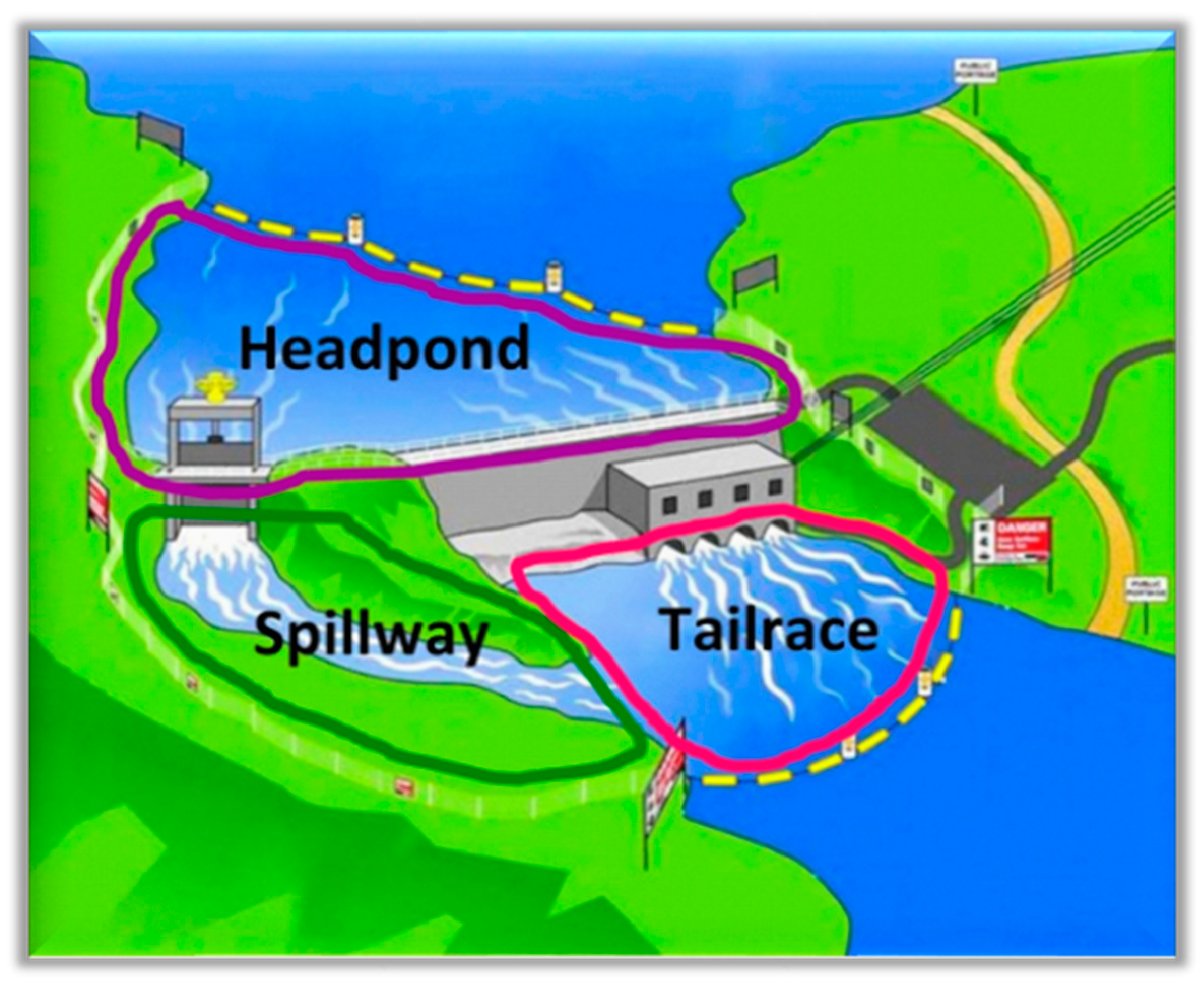
The Canadian Dam Association (CDA) guidelines [5] present a stepwise process for public-safety risk assessment around dams. The approach begins with identifying hazardous areas, as illustrated in Figure 1, which shows typical headpond, spillway, and tailrace zones where the public may be exposed to risk. These areas form the basis for further assessment, including the identification of public activities and associated hazards within each zone. Hazards are then classified, and risks are rated using a simple ordinal scale: both likelihood and consequence are scored from 1 to 5, and their product yields a risk value between 1 and 25. These scores are compared against thresholds of low, medium, or high risk, and risk treatment consists of introducing physical or operational control measures to reduce likelihood or consequence.

This methodology has value in structuring the assessment process by defining hazardous areas, documenting public activities, and providing a straightforward means of ranking risks. However, it remains qualitative in nature and relies on ordinal scales and simple multiplication, which cannot capture the complex, often non-linear relationships among hazards, exposures, and outcomes. Although ordinal approaches are widely used, their limitations are well documented [6,7,8], and they may not always provide consistent or defensible support for decision-making.

This paper addresses these limitations by introducing a quantitative framework for public-safety risk assessment and treatment around dams. The framework integrates the hazard–event–objective–control structure with the Analytic Hierarchy Process (AHP) and rating-scale elicitation to derive ratio-scale estimates of likelihood and consequence. These parameters are propagated through probabilistic simulation to quantify expected losses and uncertainty, which are then analyzed using optimization and efficient-frontier methods to identify the most cost-effective control portfolios.

Results are expressed as monetary risk metrics, enabling consistent cost–benefit comparison of mitigation options and supporting transparent, defensible prioritization of controls. The framework bridges qualitative assessments and quantitative decision-making, aligning public-safety evaluation with contemporary risk-informed and ALARP-based practices.

The remainder of this paper is organized as follows: Section 2 outlines the methodology and framework formulation; Section 3 applies the framework to a representative dam site; Section 4 discusses the results, implications for decision-making, and integration with societal risk and international tolerability frameworks; and Section 5 presents conclusions and recommendations for implementation.

2. Methodology

2.1. Framework Overview

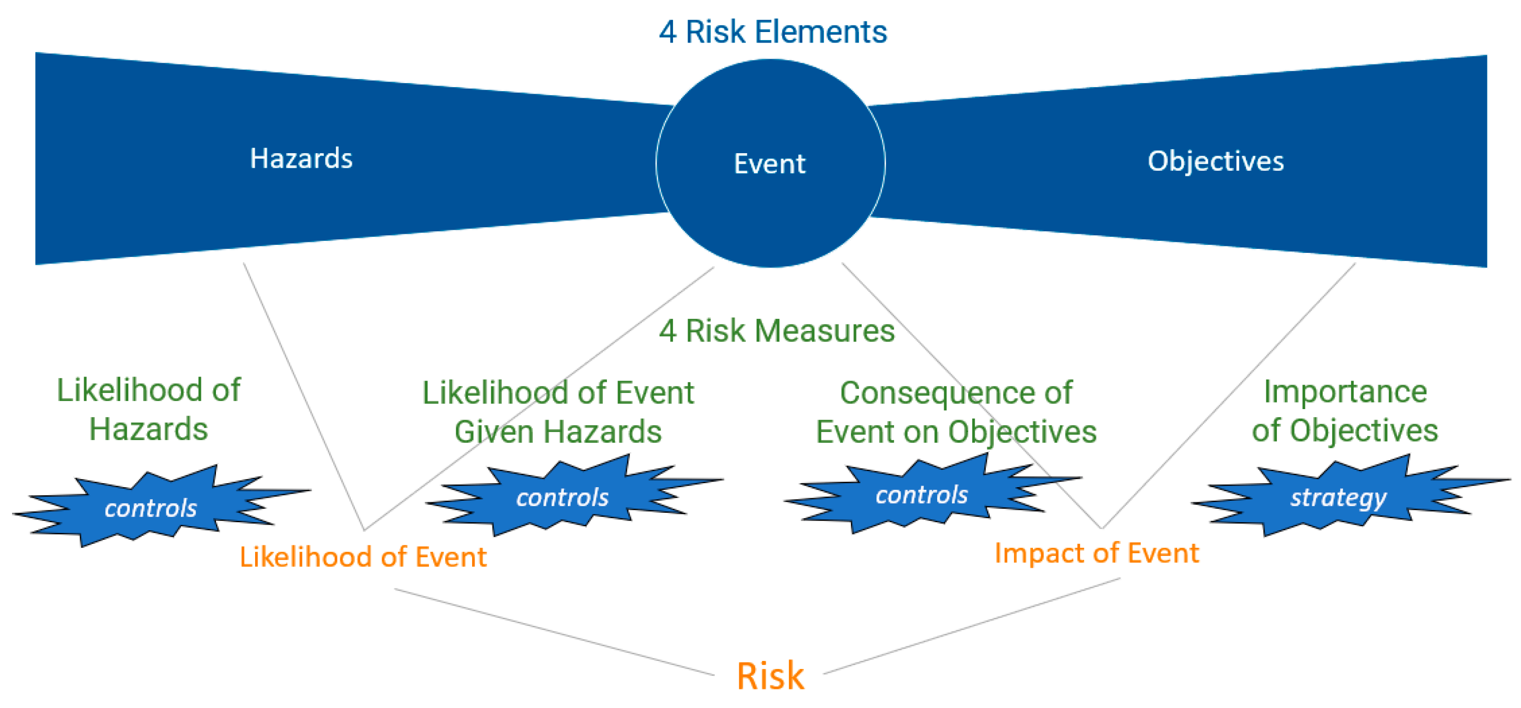
The proposed process for waterway public-safety risk assessment integrates the hazard–event–objective–control framework introduced by [9] with the Analytic Hierarchy Process (AHP). The framework identifies four fundamental risk elements—hazards, events, objectives, and controls—and three risk measures: likelihood, impact, and risk. These elements are visualized using a bow-tie diagram (Figure 2), which links causes to consequences and provides the foundation for quantitative evaluation. The AHP converts expert judgment into ratio-scale priorities through pairwise comparisons, enabling consistent quantification of likelihoods and consequences. It has been widely applied in engineering and infrastructure decision-making [10,11,12] and previously demonstrated for dam-safety risk prioritization [13,14]. Within this framework, AHP provides the structure for weighting hazards, evaluating conditional event probabilities, and estimating consequence severity across organizational objectives.

2.2. Process Outline

The overall procedure consists of nine iterative steps:

• Identify and categorize hazards.
• Map hazards to potential risk events.
• Estimate the likelihood of hazards and the conditional likelihood of events given those hazards (vulnerabilities).
• Define organizational objectives and assess their relative importance.
• Quantify event consequences for each objective.
• Compute overall event risks as the product of likelihood and consequence.
• Identify feasible control measures.
• Evaluate control effectiveness.
• Optimize the portfolio of controls to maximize total risk reduction.

These steps are implemented using the Expert Choice Riskion^® (version 6.19) decision-support platform, which automates the computation and visualization of results. The process translates qualitative insight into quantitative risk values that can be compared, communicated, and optimized.

2.3. Quantification Approaches

2.3.1. Likelihood Estimation

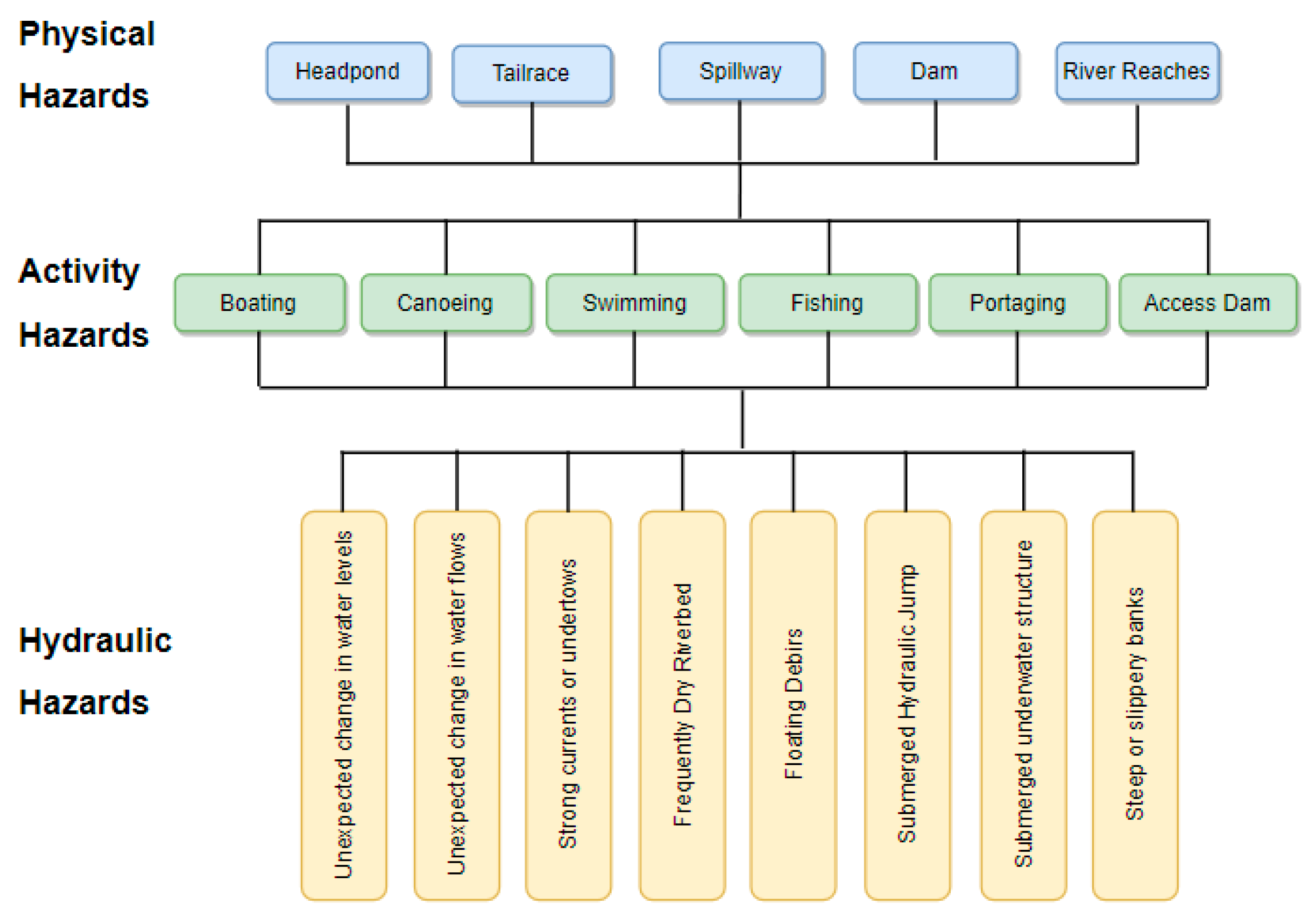
Hazards are grouped into three hierarchical levels—physical site features (e.g., headpond, spillway), activity-related hazards (e.g., boating, swimming), and operational or hydraulic hazards (e.g., rapid flow change).

• Hazard likelihoods are estimated from historical data or expert judgment as probabilities of occurrence within a defined period.
• Conditional event likelihoods, P(Event|Hazard), represent system vulnerability and are derived using AHP-based pairwise comparisons or direct rating scales, and where data permit, through probabilistic models such as Monte Carlo sampling.
• Event likelihoods are synthesized from hazard and conditional probabilities to represent total exposure.

This structure ensures traceability from physical causes to probabilistic event representation.

2.3.2. Consequences and Objectives

Consequences are quantified in relation to defined objectives, which represent valued outcomes potentially affected by hazardous events (e.g., public safety, public trust, operational disruption) The quantification process includes:

• Objective importance: Each objective is weighted based on its relative importance to stakeholders using AHP pairwise comparisons. These weights ensure that risk estimates reflect organizational priorities.
• Impact measurement: Consequences of events on each objective are quantified as fractional reductions in objective value or as monetary losses where possible. This includes metrics such as fatalities, injuries, economic costs, or service disruptions.

The event impact is then calculated as the product of event consequences and the importance of each objective. This ensures that resulting impact measures reflect both the severity of outcomes and their strategic significance.

2.3.3. Risk Computation and Estimates

Once likelihoods and consequences are quantified, risk is computed as the expected loss to each objective:

R = P(E) × C(E)

(1)

where P(E) is the event probability and C(E) the corresponding consequence. The aggregation of risks across all events yields the total risk profile for the site. When objective values are expressed monetarily, the results can be interpreted directly in economic terms, enabling cost–benefit and optimization analyses.

2.4. Addressing Non-Linearities Through Monte Carlo Simulation

Assessing public-safety risk around dams involves complex interactions among numerous hazards, potential events, and organizational objectives. Traditional deterministic approaches—where expected likelihoods and impacts are multiplied to compute expected risk—often fail to capture these complexities due to the flaw of averages [15]. Such methods assume linear relationships and independence among risk factors, assumptions that seldom hold in practice [16,17].

Non-linear behavior arises when multiple hazards contribute to the same event, when events interact to affect shared objectives, or when sequential impacts compound over time. For example, a single event triggered by several hazards should be counted only once, and repeated impacts on the same objective should reduce its remaining value rather than be summed [18,19]. To address these challenges, Monte Carlo simulation provides a robust probabilistic framework for modeling uncertainty and capturing the full range of possible outcomes [20,21].

In this framework, the system is simulated through thousands—or tens of thousands—of trials, each representing one possible realization of hazard occurrences, event triggers, and resulting consequences over a defined time frame. Random numbers drawn from a uniform distribution are compared with computed probabilities to determine whether hazards occur in each trial. Conditional probabilities govern event occurrence given specific hazards. When events occur, their consequences are applied to associated objectives, with reductions to objective values compounded across multiple impacts rather than treated as additive. This structure captures the inherently non-linear and interdependent behavior of dam-safety risk scenarios.

The simulation framework accommodates a large number of hazards and event pathways, potentially exceeding one hundred hazards, and records outputs such as total losses, frequency distributions, and cumulative exceedance probabilities. These results are used to construct loss-exceedance curves (LECs)—showing the probability that losses exceed given thresholds—and Value-at-Risk (VaR) metrics, which quantify the magnitude of potential losses at selected confidence levels. LECs and VaR are widely applied in probabilistic risk assessment and financial risk management to express tail-risk behavior and decision confidence [16,22,23]. Their adaptation to dam-safety analysis provides a transparent way to visualize and quantify both expected and extreme loss potential under uncertainty.

In this study, all simulation operations—including random sampling, event triggering, conditional-probability evaluation, and risk-metric generation—were implemented using the Expert Choice Riskion^® (version 6.19) decision-support platform. The software automates the iterative trial structure and output generation, ensuring that the resulting probabilistic risk characterization is both robust and reproducible. The simulation framework described above was subsequently applied to the case-study dam to evaluate risk distributions, convergence behavior, and loss-exceedance characteristics, the results of which are presented in Section 3.

2.5. Risk Treatment and Control Optimization

Risk treatment refers to the process of identifying and implementing measures to modify risk and achieve an acceptable level of public safety. In dam safety, this involves controls that act on the risk pathway to reduce the likelihood of hazardous events, limit vulnerability once an event is initiated, or mitigate the resulting consequences. This step corresponds to the treatment stage of the ISO 31000 risk-management framework and the guidance outlined in [5].

Controls are classified according to the element of the risk pathway they influence:

• Likelihood-reducing controls act on the hazard source to prevent or reduce its probability of occurrence, such as barriers, booms, or fences.
• Vulnerability-reducing controls reduce the susceptibility of people or systems once a hazard exists, for example through alarms, surveillance, or operational protocols.
• Consequence-reducing controls limit the severity of outcomes once an event has occurred, such as rescue procedures or rapid-shutdown mechanisms.

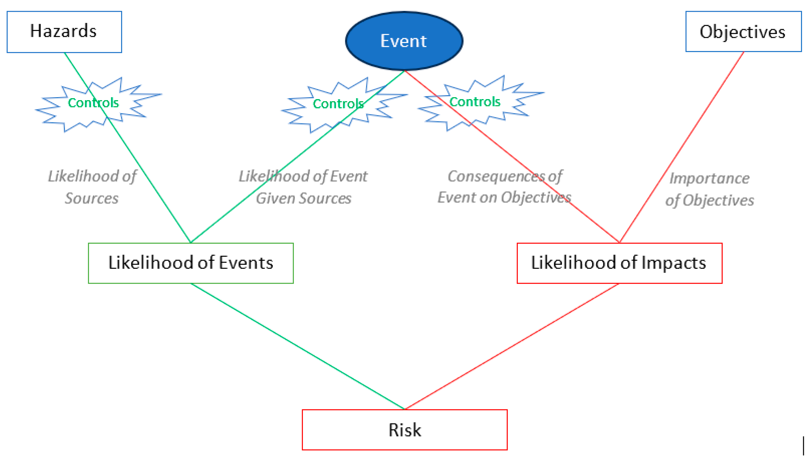
Figure 3 illustrates how these controls operate at different points along the risk pathway: likelihood-reducing controls act at the hazard stage, vulnerability-reducing controls between the hazard and event nodes, and consequence-reducing controls after event initiation to limit loss severity.

To further illustrate the range of typical public-safety controls and their conceptual placement along the pathway, each control is represented in the model by its effectiveness, expressed as a fractional reduction applied to the relevant parameter of the risk equation—likelihood, vulnerability, or consequence. When data are unavailable, effectiveness estimates are derived from expert judgment or analogous applications and represented as probability distributions to capture uncertainty [16,17].

Because multiple controls may influence the same pathway element, their combined effect is not assumed to be additive. Dependencies and overlaps are handled through conditional relationships to avoid overstating total risk reduction. During Monte Carlo simulation, control-effectiveness values are sampled in each trial, allowing uncertainty in performance and interaction to propagate naturally through the results.

This formulation ensures that control measures are consistently represented within the probabilistic framework and directly linked to the quantitative assessment of risk. The next section applies this structure to a representative dam site, where specific control measures are modeled and their combined influence on public-safety risk is evaluated.

Table 1. Representative control functions and targeted components of the risk pathway.

Control Measure	Type	Risk Pathway Target (H-V-C)
Signage	Physical	H-C
Safety Booms	Physical	H-C
Fencing/Barricades	Physical	H-C
Audible or Visual Signaling Devices	Physical/Operational	H-V-C
24/7 Video Surveillance	Operational	V
Operational Controls (Procedures)	Operational	V-C
Security Patrols	Operational	H-C
Public Education and Outreach	Educational	H-C
Written Notification to Property Owners	Educational	H-C

H = Hazard likelihood; V = Event vulnerability; C = Consequence Severity.

summarizes representative measures, their nature (physical, operational, or educational), and the components of risk they target.

3. Results (Application to Case Study Dam Site)

3.1. Case Study Overview

The framework was applied to a representative dam site featuring typical components—headpond, spillway, and tailrace—along with public access areas. The goal was to demonstrate how the framework translates qualitative insights into quantitative, decision-relevant results across the risk pathway: hazard identification → event likelihood → consequence estimation → risk quantification → control optimization.

3.2. Hazards and Risks Characteristics

The framework was applied to the case study dam site to identify key hazards, risk events, and their potential impacts on organizational objectives. The results below summarize the main findings from this stage of the analysis.

3.2.1. Hazard Categories

Hazards around a dam can be categorized as activity hazards, situational (hydraulic) hazards, physical hazards, and operational/procedural hazards. This hazard classification was developed by the authors as part of this study to provide a structured basis for systematic risk evaluation using AHP. The hazards described below were informed in part by established dam safety references, including the CDA’s Guidelines for Public Safety Around Dams [5] and the ASDSO’s Public Safety Hazards guidance [24]. We begin by presenting the identified hazards and estimating their likelihoods, followed by the likelihoods of risk events conditioned on those hazards, and finally the impacts of these events on defined objectives.

• Physical hazards—inherent features of the dam environment, including the presence of spillways, discharge structures, submerged infrastructure, steep banks, or confined reaches.
• Activity Hazards—recreational or human activities that can initiate risk events (e.g., boating, canoeing, swimming, portaging, fishing, and accessing dam structures).
• Hydraulic hazards—situational conditions resulting from dam operations, such as unexpected changes in water levels or flows, strong currents, submerged hydraulic jumps, or floating debris. These may be visible, deterring public exposure, or hidden, leading to significantly higher exposure likelihoods.
• Operational hazards—conditions introduced by operational procedures, such as automatic gate operations or remote flow controls, which can abruptly alter hydraulic conditions.

The identified hazards are structured into a three-level hierarchy (Figure 4), linking physical site conditions to activities and operational scenarios. This hierarchical view facilitates systematic risk evaluation and ensures that hazards are traced from their source through to potential exposure and impact.

Although operational and procedural hazards, such as automatic gate operations or remote flow control actions, were not included in this case study because they were not applicable to the selected example, the framework can readily incorporate them where relevant. In such cases, they would be treated as additional sources within the hazard hierarchy and assessed in the same manner, with likelihoods estimated based on operational data and potential consequences mapped to downstream public safety objectives.

3.2.2. Risk Events

From a public safety perspective, several types of risk events can occur around dams, most of which involve direct interaction between the public and hazardous conditions. These events represent the outcomes that matter most for risk management, as they lead to tangible losses—often in the form of fatalities. The case study considers the following representative public safety risk events:

• Loss of control of power boat resulting in fatality.
• Loss of control of canoe resulting in fatality.
• Inability to surface or control direction while swimming resulting in fatality.
• Falling into water while portaging resulting in fatality.
• Falling into water while fishing resulting in fatality.
• Jumping or falling from dam structure resulting in fatality.

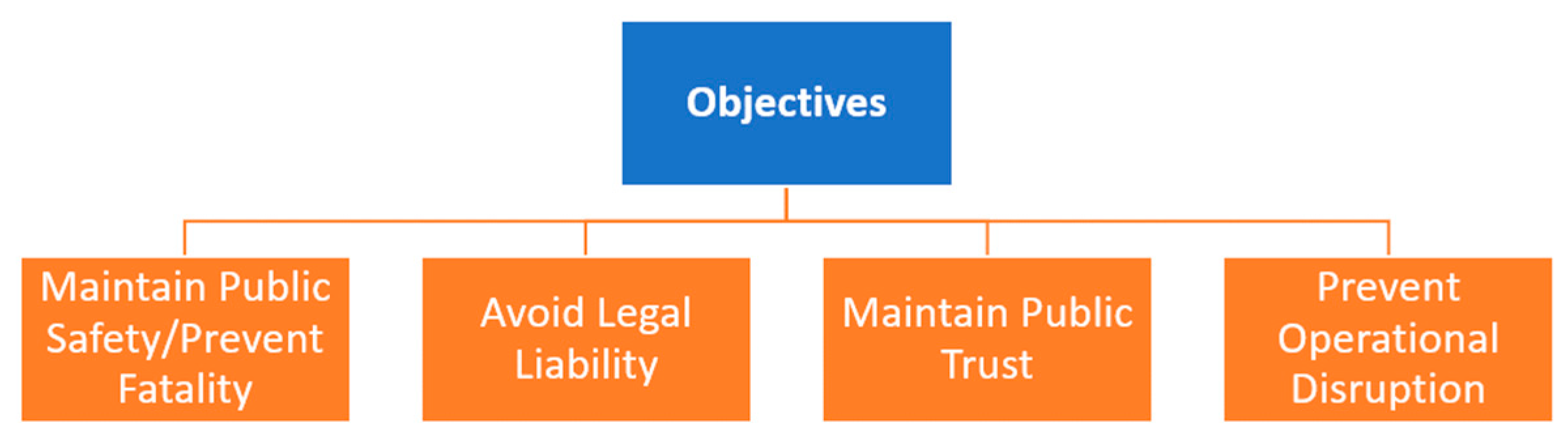
3.2.3. Objectives

Each risk event has the potential to cause losses to one or more of the dam owner’s organizational objectives. These objectives, typically structured in a hierarchical form, capture the key outcomes that the organization seeks to protect. For the purpose of this study, only the highest-level objectives are considered (Figure 5).

The relative importance of these objectives is organization-specific and reflects factors such as mission, strategic priorities, and stakeholder expectations. Their weights are derived through pairwise comparisons following the AHP, allowing subjective judgments to be expressed as ratio-scale priorities that can be integrated into quantitative risk assessments.

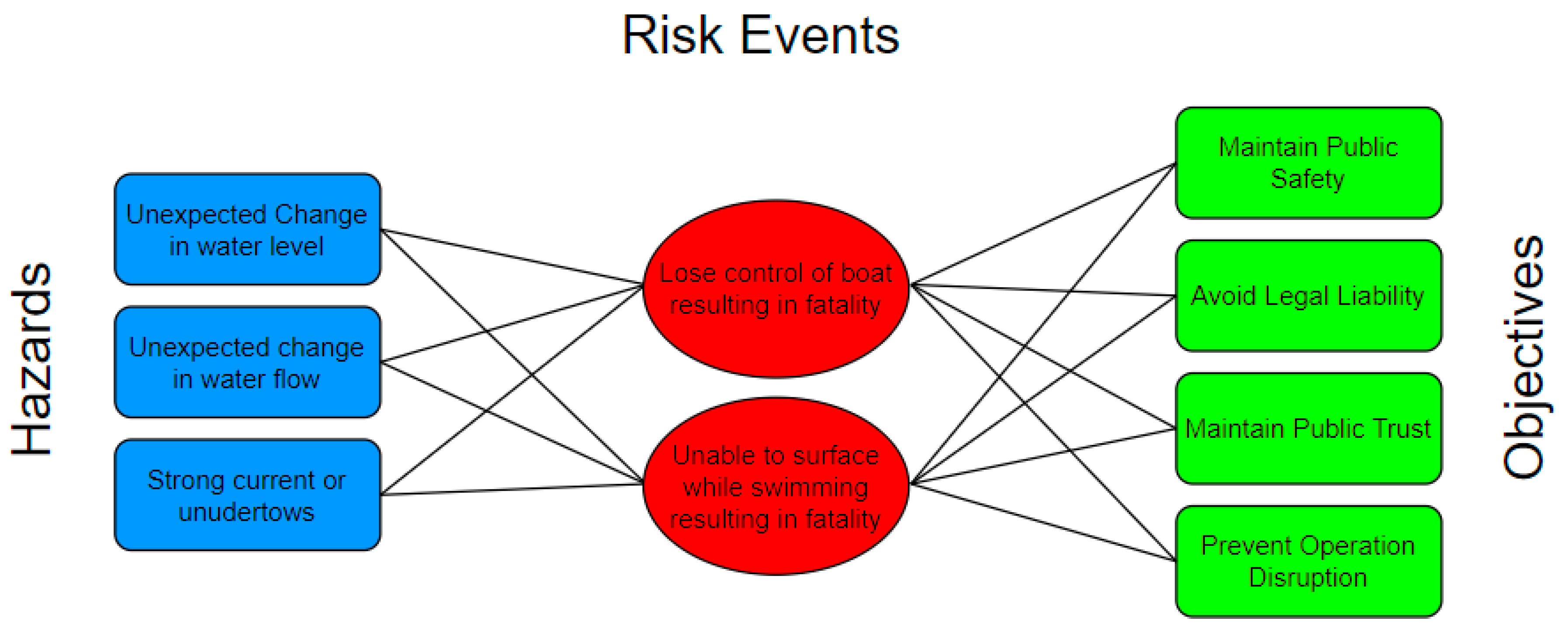
3.2.4. Mapping Hazards to Events and Events to Objectives

Each hazard identified earlier can give rise to one or more risk events, and conversely, a single event can be triggered by multiple hazards. For example, the event “inability to surface while swimming” can be caused by unexpected changes in water level, rapid changes in flow, or strong subsurface currents. Likewise, the hazard “unexpected change in water flow” can trigger several distinct events, including loss of control of a canoe or power boat.

Similarly, individual events can affect multiple objectives, and each objective may be impacted by several different events. These complex many-to-many-to-many relationships—between hazards and events, and between events and objectives—are illustrated in Figure 6. Their complexity makes traditional spreadsheet-based approaches inadequate.

To handle this complexity, specialized decision-support software such as Riskion^® (version 6.19) is employed to organize, synthesize, and compute likelihoods, consequences, and impacts within this interconnected system. This approach ensures that the risk assessment remains comprehensive, traceable, and defensible.

3.3. Risk Evaluation Outputs

3.3.1. Hazard Likelihood Estimation

Hazard likelihoods were evaluated across the three levels of the hazard hierarchy: physical, activity-related, and hydraulic.

Physical Hazards:

The presence of first-level physical hazards such as the headpond, spillway, and tailrace is deterministic and therefore represented by binary likelihoods (0 or 1) depending on whether each element exists at the site.

Activity Hazards:

Second-level activity hazards were modeled as Poisson processes based on historical activity rates. Using observed annual frequencies, the probability of at least one occurrence within a 10-year period was calculated as:

P(≥1) = 1 − e^−λt

(2)

where λ is the observed annual occurrence rate and t is the timeframe. Results (

Table 2. Yearly rates of activity hazards with all likelihoods assumed to occur at least once within a 10-year period.

Activity Hazard	Headpond	Spillway	Tailrace	Dam Structures
Boating	5	16	18	-
Canoeing	20	8	6	-
Swimming	20	6	7	-
Portaging	30	15	12	-
Fishing	15	28	22	-
Accessing Dam	-	-	-	5

All listed activity rates correspond to probabilities exceeding 99% over the 10 year analysis period.

) show that all major recreational activities, including boating, swimming, portaging, and fishing, have a near-certain probability (>99%) of occurring within a 10-year period in areas accessible to the public.

Hydraulic Hazards Likelihoods and Exposure Results

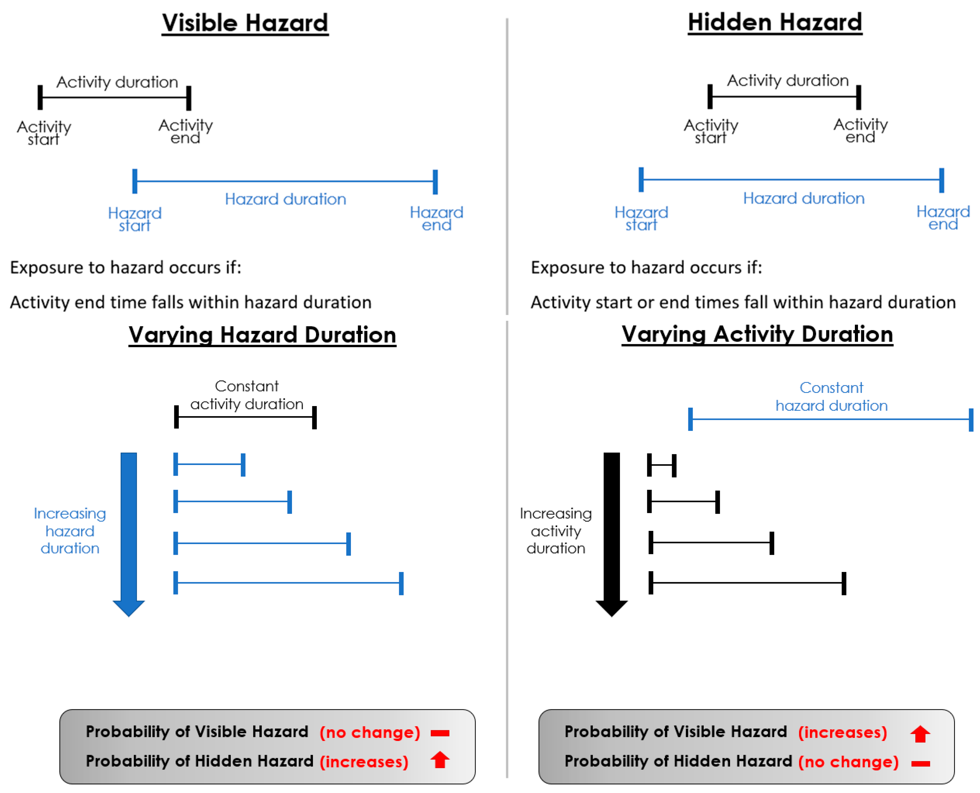
Hydraulic hazards resulting from dam operations are a major contributor to public safety risk, particularly when sudden changes in flow or water level occur during recreational activities. These hazards can be broadly classified as visible (e.g., turbulent flows or surface disturbances) or hidden (e.g., subsurface currents or flow changes without visual indicators). The distinction is significant, as hidden hazards lead to much higher exposure probabilities due to the reduced ability of recreationists to recognize and avoid them. Figure 7 illustrates how variations in activity duration and hazard duration influence exposure likelihood for visible versus hidden hazards.

To quantify exposure likelihoods, a Monte Carlo simulation was conducted based on random variations in four variables: (i) the start time of public activities, (ii) the duration of those activities, (iii) the occurrence time of hydraulic changes, and (iv) their duration. Overlaps between activity periods and hazard windows were used to estimate exposure probabilities. Simulations assumed that public interaction with the site occurs between 07:00 and 20:00, reflecting typical usage patterns.

The raw output of the simulation is the probability of overlap within a single day. To translate this into a 10-year exposure likelihood—the timeframe adopted for this analysis—the daily overlap probability was first divided by 365 to represent an annualized exposure rate. This value was then multiplied by the estimated number of recreationists per activity type over the 10-year period. This conversion allows the results to reflect the cumulative probability that at least one individual will be exposed to a hydraulic hazard over the project’s analysis horizon.

The simulation results in

Table 3. Assumptions used in Monte Carlo simulations to estimate likelihoods of being exposed to unexpected change to hydraulic hazards (change in water level or flow) while performing certain activities.

Assumptions	Headpond Activity				Operation
	Swimming/ Wading	Boating	Canoeing	Fishing from Land	Spilling	Generation
Number of recreationists per 10 year (N)	20	5	20	15
Timeframe (T)	10 years
Occurrence Period	7:00 a.m.–8:00 p.m.
Occurrence Mean	12:00 p.m.
Std. Dev. Of Occurrence (hours)	6	8	8	10	6	6
Mean of Duration of Activity (hours)	1	2	2	4	7	7
Std. Dev. Of Duration (hours)	0.3	1	1	1	1	1
Distribution Type	NORMAL
Likelihood of hazard exposure (L)	12%	17%	17%	27%	Obtained from MC simulations
Annual Likelihood of unexpected change in water flow during activity	6.58 × 10−2	2.33 × 10−2	9.32 × 10−2	1.64 × 10−2

highlight two key insights:

1.

Effect of Duration: The duration of both activities and hazards plays a critical role in determining exposure probability.

○

For visible hazards, exposure occurs only if an activity is already in progress when the hazardous condition is present. Longer activity durations therefore increase the probability of exposure, while the duration of the hazard itself has little effect, since the hazard is apparent and recreationists can typically avoid initiating activities in unsafe conditions.

○

For hidden hazards, exposure occurs when activity start or end times fall within the hazard period. In this case, the duration of the hazard is the dominant factor: the longer the hazardous condition persists, the greater the likelihood that recreational activities will overlap with it.

2.

Effect of Visibility: The results underscore the critical importance of hazard visibility. The likelihood of exposure to a hidden hazard during swimming activities was estimated at approximately 55%, compared to only 2% for a visible hazard. This dramatic difference demonstrates why visibility must be explicitly considered in risk assessments and control strategies.

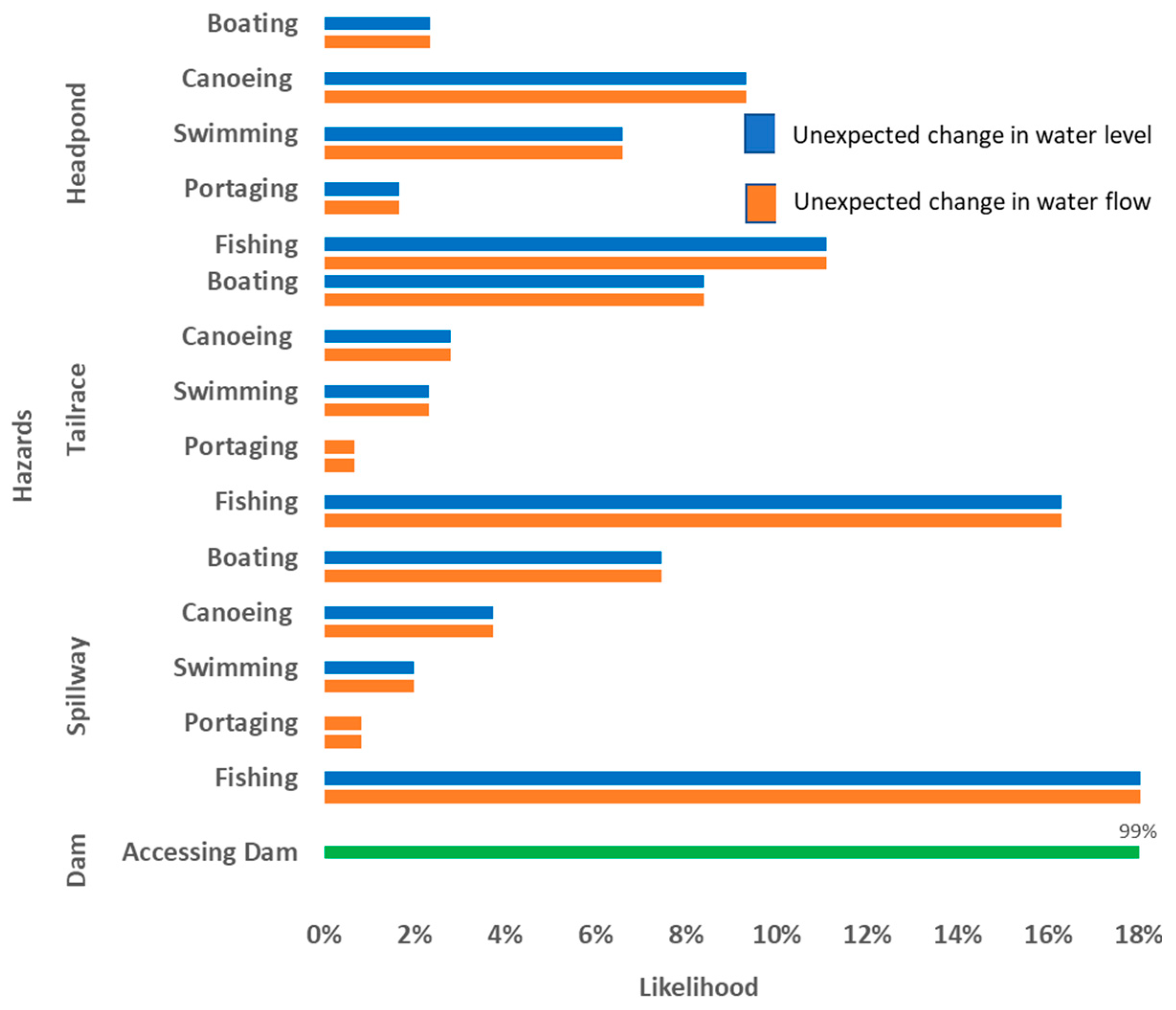
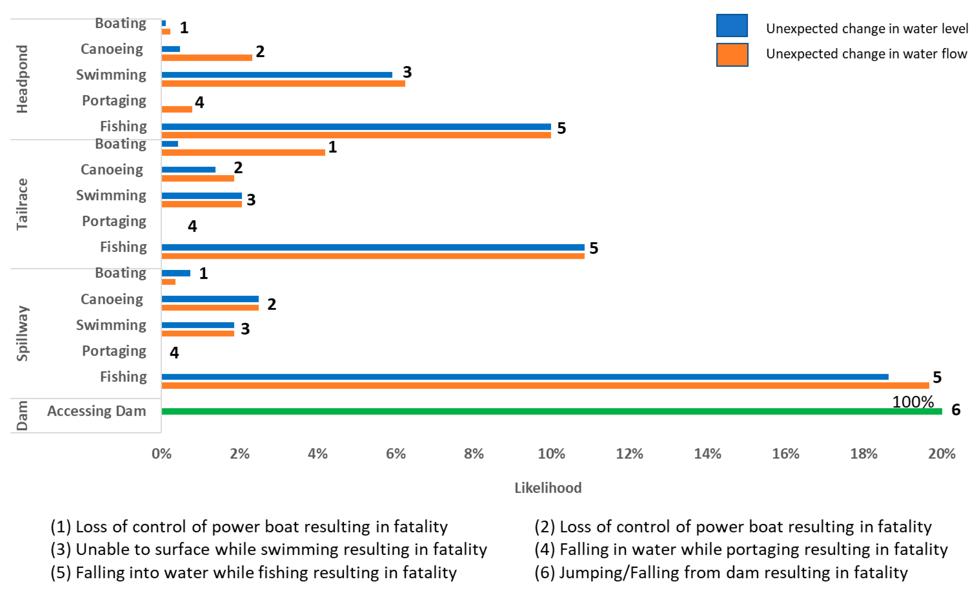
The synthesized likelihoods of two key hydraulic hazards, unexpected changes in water level and water flow, are shown in Figure 8. In this example site, the two hazards exhibit nearly identical likelihoods because the reservoir, spillway, and tailrace volumes are relatively small, meaning changes in flow and water level occur almost simultaneously. In systems with larger headpond storage, however, these two conditions may diverge significantly, with water flow changes occurring independently from sudden level fluctuations.

3.3.2. Measurement of Event Likelihoods Given Hazards (Vulnerabilities)

Once hazard likelihoods have been estimated, the next step is to quantify the conditional likelihood that a risk event will occur given the presence of those hazards—referred to as the vulnerability of events to hazards. This parameter captures how exposure translates into actual outcomes and is a critical component in computing overall risk.

Vulnerability estimation was carried out using expert judgment methods implemented in Riskion^® (version 6.19). The primary approach relies on pairwise probability comparison, where experts assess the relative likelihood of two probabilities (for example, whether a 10% probability is more likely than a 50% probability, and by how much). These judgments are synthesized using the AHP, which converts qualitative comparisons into ratio-scale quantitative estimates. When multiple experts contribute judgments, a geometric average is applied to preserve ratio properties and reduce individual bias. This approach has been shown to produce remarkably accurate results, as the eigenvector-based synthesis averages out judgment errors and captures underlying preference intensities.

A simpler but less precise alternative is the use of a rating scale (

Table 4. Likelihood intensity scale used for hazard occurrence assessment.

Intensity Name	Value (%)	Description
Almost certain	99.00	Almost certain to occur
Highly likely	95.00	Highly likely to occur
Very likely	90.00	Very likely to occur
More than likely	80.00	More than likely to occur
Likely	66.67	Likely to occur
Fifty–fifty	50.00	Fifty–fifty to occur
One in four	25.00	One in four to occur
Somewhat unlikely (one in ten)	10.00	Somewhat unlikely (one in ten) to occur
Unlikely (one in twenty)	5.00	Unlikely (one in twenty) to occur
Highly unlikely	1.00	One in a hundred
Extremely unlikely	0.10	One in a thousand
Will never happen	0.00	Virtually impossible

), where experts select a likelihood category (e.g., “likely,” “highly unlikely”) that corresponds to a predefined numerical probability. This approach is faster and still provides useful estimates, particularly in early-stage assessments.

Table 5. Vulnerability of events to hydraulic hazards and rationale for assigned values.

Hazard	Location	Vulnerability of Event to Hazard (%)	Reason/Comment
Unexpected change in water level	Headpond	5.00	Very large reservoir with slow and gradual level changes during spilling and generation. Resulting hydraulic conditions are not considered hazardous enough to trigger the event.
	Tailrace	50.00	Sudden elevation changes and turbulent, aerated flow may cause canoers to lose balance due to hydraulic conditions.
	Spillway	66.67	Rapid changes in water level can sometimes cause a canoe to capsize.
Unexpected change in water flow	Headpond	25.00	Very large reservoir with slow and gradual changes in water level during spilling and generation.
	Tailrace	66.67	Highly turbulent and aerated flow may cause a canoe to sink.
	Spillway	66.67	Very turbulent and fast flow likely to cause canoe capsizing.

presents an example of vulnerability estimates for the event “Loss of control of canoe resulting in fatality” under various hazard conditions. Vulnerability differs substantially across contexts. For instance, a sudden water level change in the headpond is associated with low vulnerability due to the large reservoir volume and gradual hydraulic transitions, whereas abrupt flow changes in the spillway can frequently result in canoe capsizing.

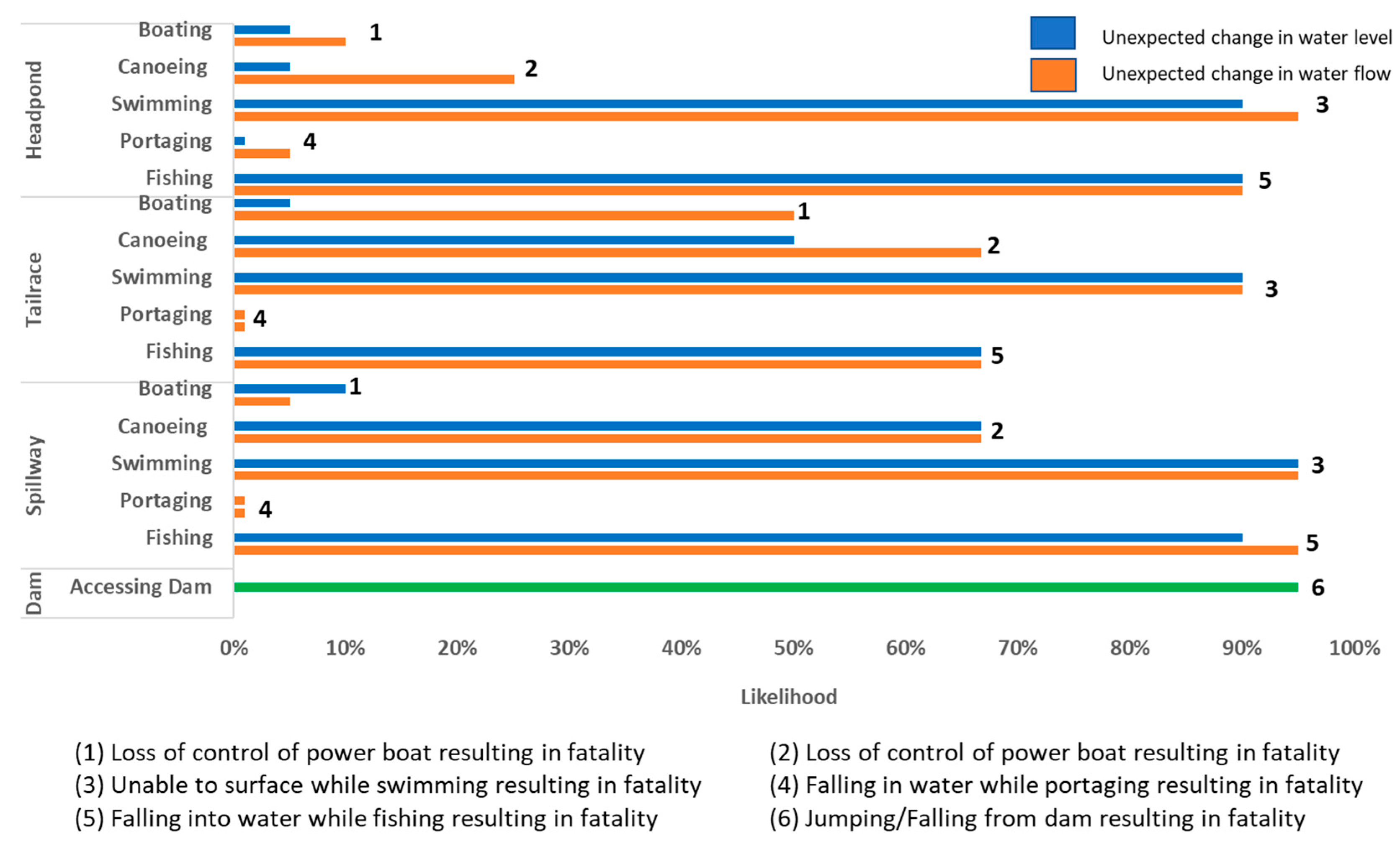
Figure 9 illustrates these conditional vulnerabilities for two representative hazards—unexpected changes in water level and flow—during power boating.

To demonstrate how hazard likelihoods and event vulnerabilities interact to produce overall event probabilities, Figure 10 presents synthesized results for two representative hydraulic hazards—unexpected changes in water level and water flow—across various public activities. The results highlight how activity–hazard interactions influence risk profiles, with certain combinations (such as fishing or swimming during flow changes). These outputs provide a critical bridge between hazard characterization and quantitative risk evaluation, forming the foundation for the overall synthesis of event likelihoods presented in Figure 11.

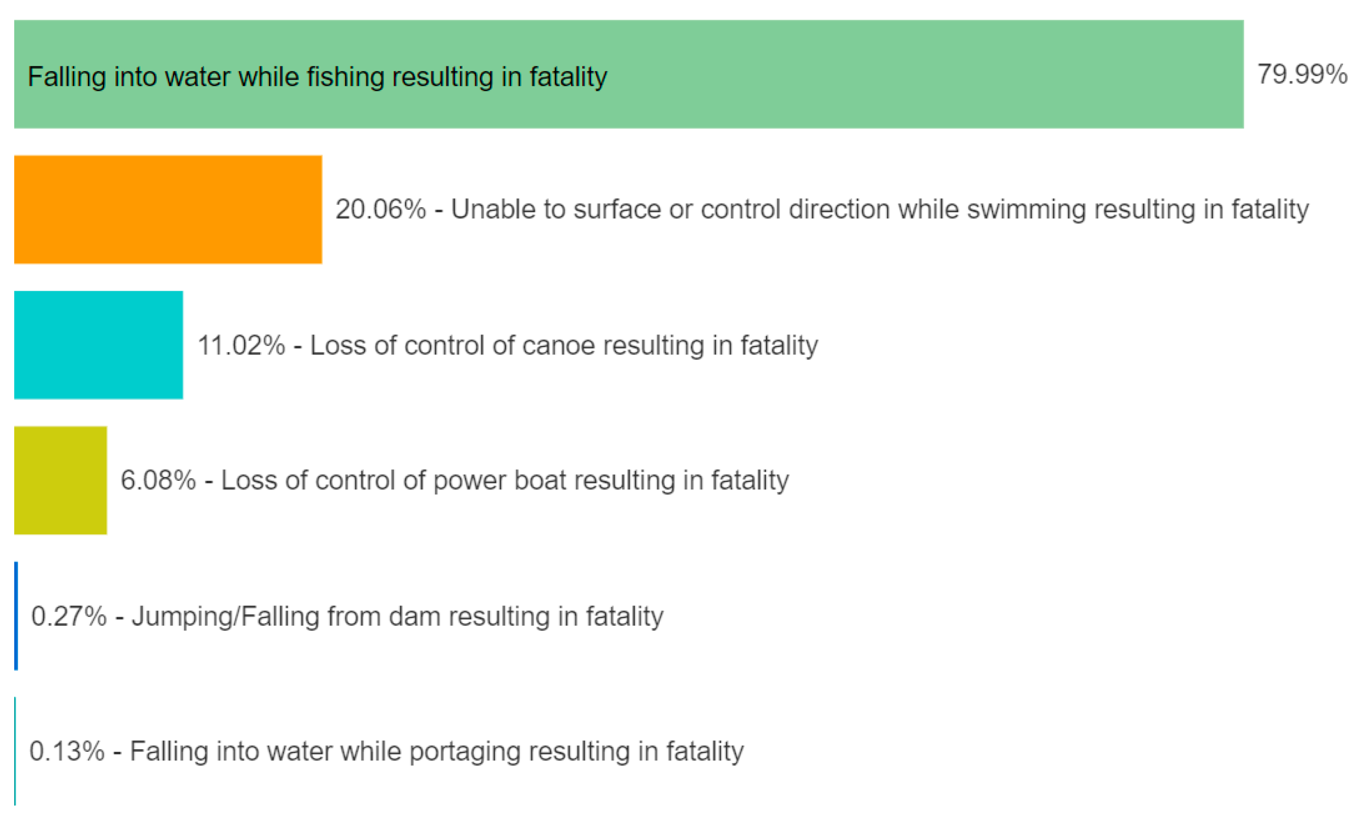
3.3.3. Event Likelihoods

The overall likelihood of each risk event is calculated by synthesizing two key components: the likelihood of the initiating hazards and the conditional likelihood of events given those hazards (vulnerabilities). This synthesis is performed within the Riskion^® (version 6.19) platform by computing the sum product of these two estimates, ensuring that the resulting event probabilities maintain ratio-scale integrity and accurately represent the underlying risk relationships.

Figure 11 presents the aggregated event likelihoods for the case study dam site, integrating the hazard occurrence probabilities with expert-derived vulnerability judgments. These results provide a comprehensive view of which events are most probable under existing site conditions and serve as a critical input for subsequent consequence assessments and risk quantification.

3.3.4. Importance of Objectives

While likelihoods and consequences are objective in nature, the importance of objectives is inherently subjective and reflects the mission, strategy, and values of the organization. Two organizations exposed to similar risks may prioritize objectives differently. For example, a software start-up might place higher importance on short-term revenue, whereas a large utility may prioritize public trust or legal compliance.

To quantify these subjective priorities, the AHP is used to derive ratio-scale weights for each objective based on pairwise comparison judgments. This process allows decision-makers to express relative importance in a structured way, and if multiple experts provide input, their judgments are combined using a geometric average to maintain ratio-scale consistency.

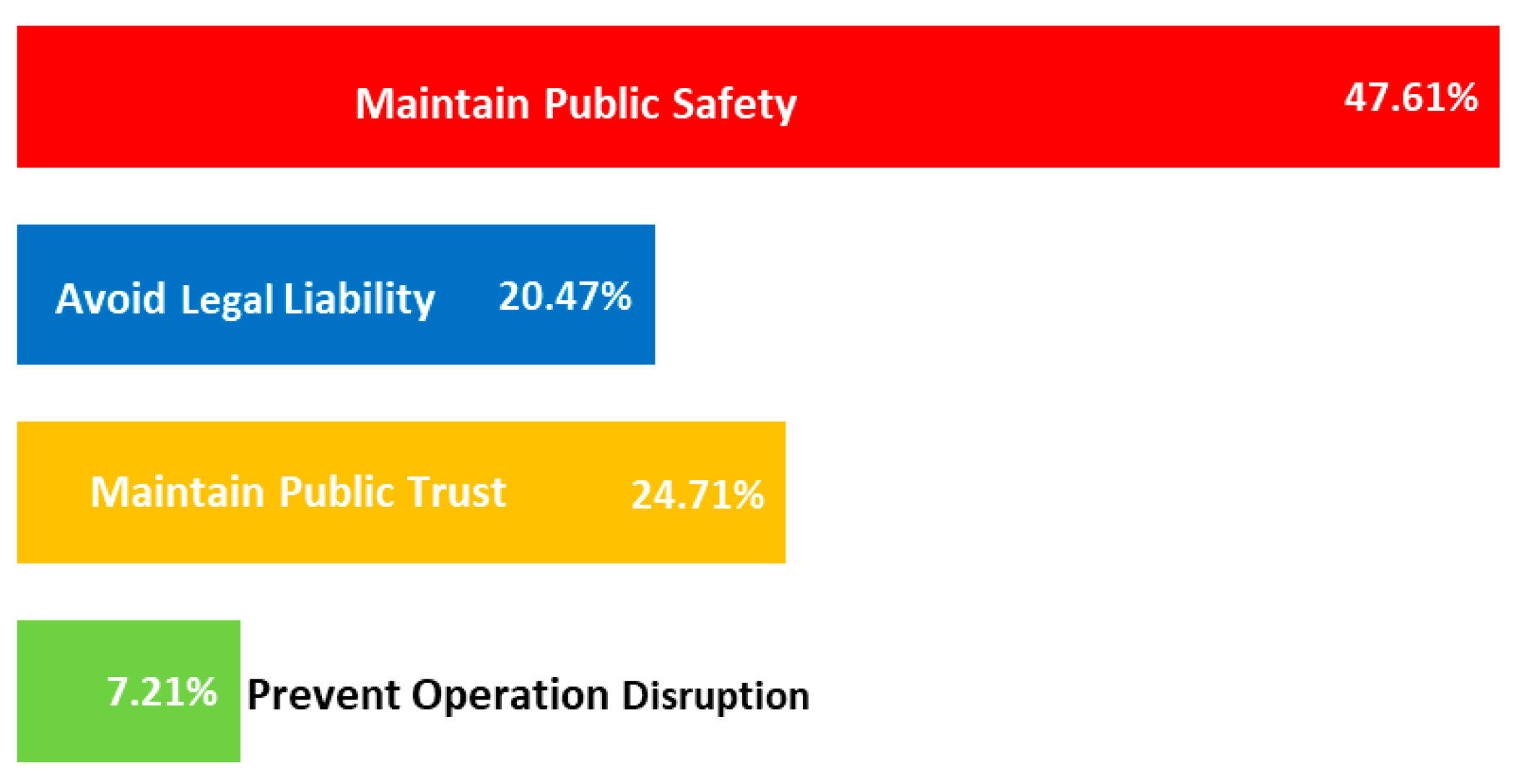
Figure 12 presents the resulting priority weights for the case study organization’s top-level objectives, which form the basis for computing event impacts and overall risk estimates in the following sections.

3.3.5. Measurement of Event Consequences to Objectives

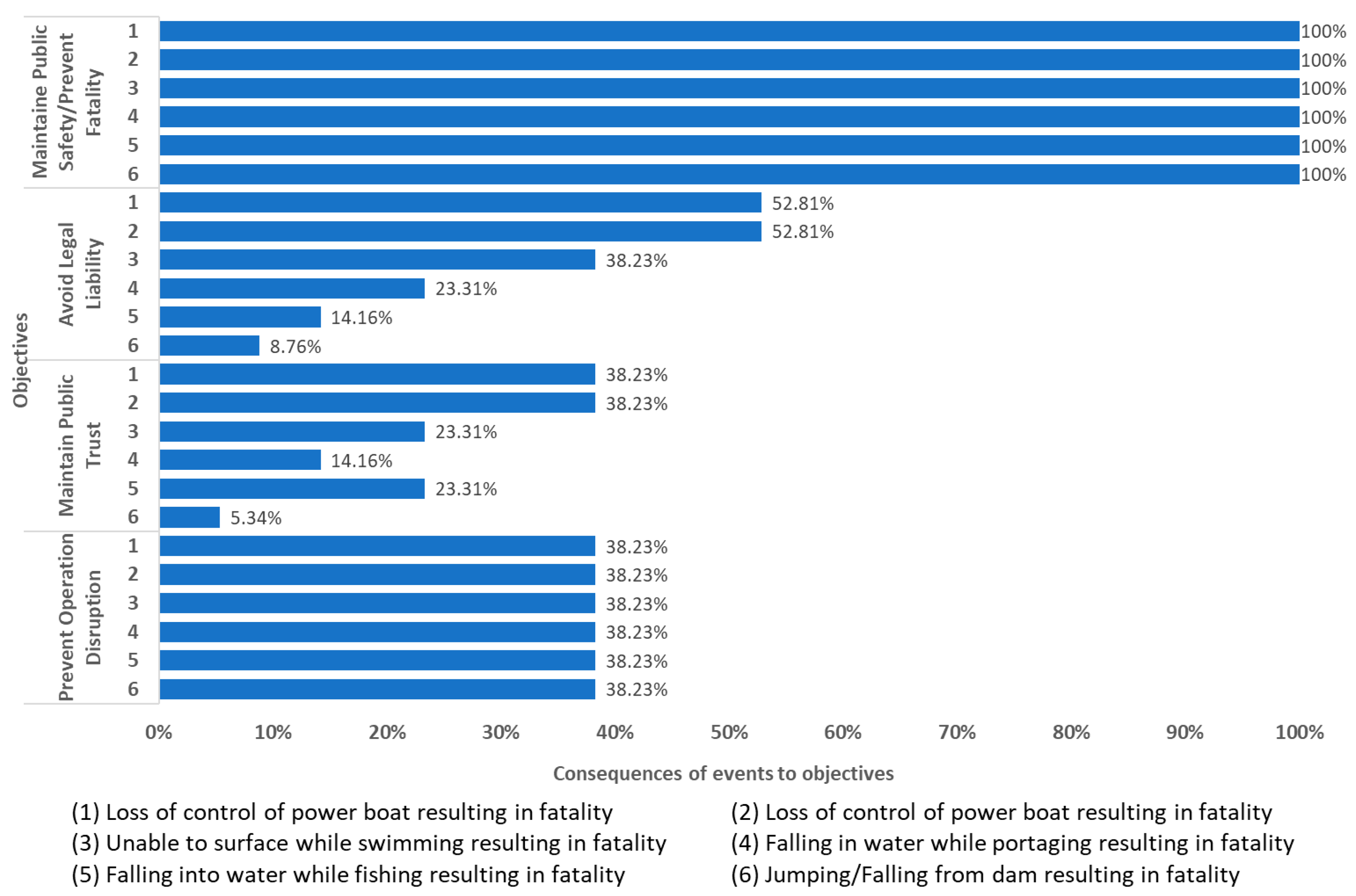
The consequences of risk events on organizational objectives represent the severity of their potential outcomes. These consequences are assessed through expert judgment, where each event is evaluated against each objective to determine the extent of its impact. A structured rating scale is used to ensure consistency and comparability in these judgments.

Table 6. Rating Scale for Consequences of Events on Objectives.

Intensity Name	Value	Description
Extreme	100%	Detrimental impact on organization objective
Significant to extreme	84.03%	Extreme impact on organization objective
Significant	71.36%	Significant impact on organization objective
Considerable to significant	59.84%	Extreme impact on organization objective
Considerable	52.81%	Considerable impact on organization objective
Moderate to considerable	38.23%	Moderate to considerable impact on organization objective
Moderate	23.31%	Moderate impact on organization objective
Low to moderate	14.16%	Low/moderate impact on organization objective
Low	8.76%	Low impact on organization objective
Very Low	5.34%	Very low impact on organization objective
Just a tad	2.60%	Extremely low impact on organization objective
Insignificant	1.16%	Insignificant impact on organization objective
None	0.00%	No impact to the organization objective

presents an example of the consequence rating scale used in this study. Each intensity level corresponds to a percentage value that reflects the degree of detriment the event could cause to an objective, ranging from “None” (0%) to “Extreme” (100%).

The consequence of each event is estimated for every objective individually. These values provide a basis for quantifying how different types of events, such as fatalities due to loss of vessel control or accidental falls, affect key organizational goals. Figure 13 illustrates the resulting consequence profiles for the considered risk events relative to the organization’s top-level objectives.

3.3.6. Measurement of Event Impacts

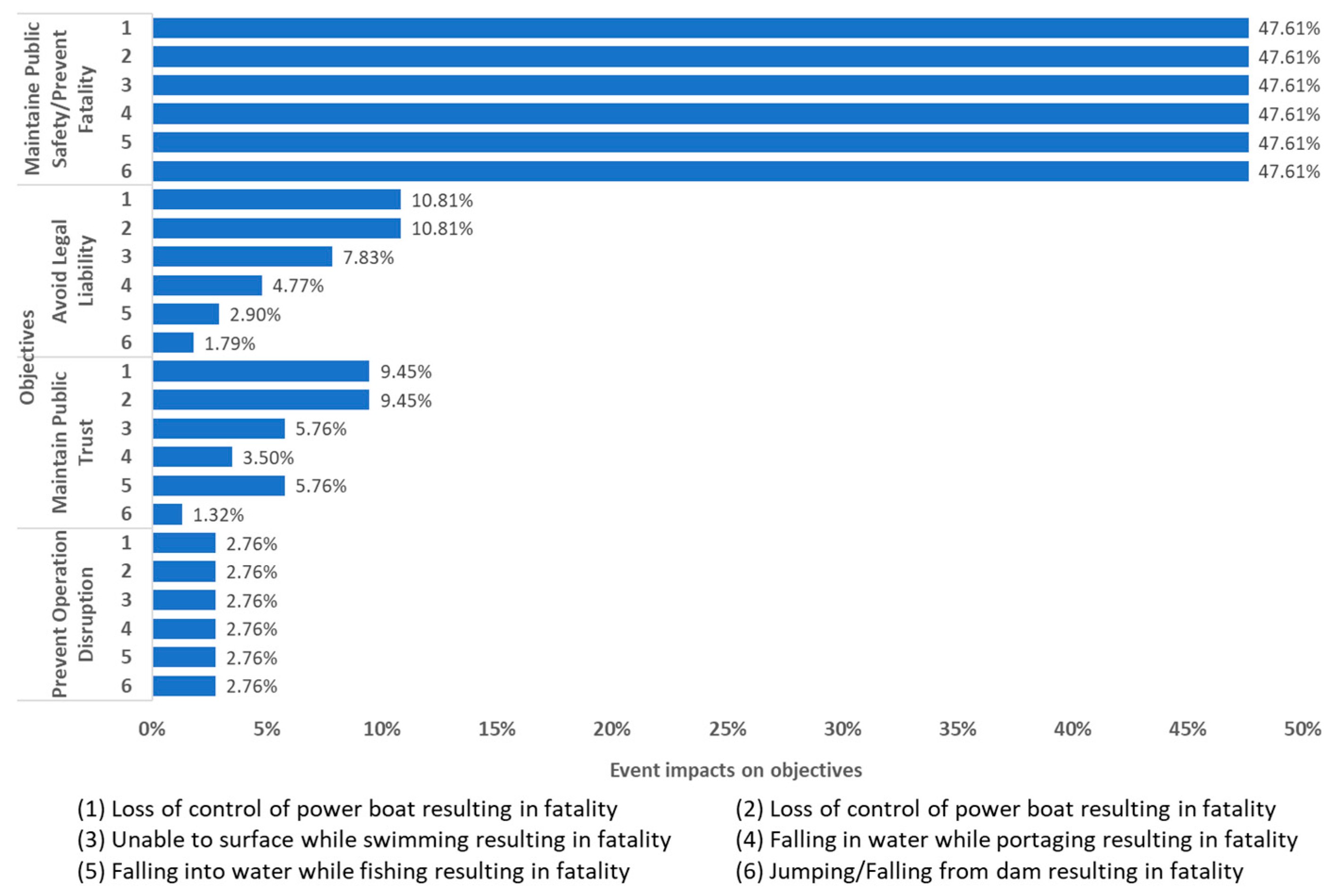
The impact of a risk event on organizational objectives combines two essential components: the consequence of the event for each objective and the relative importance (or weight) of that objective. As shown conceptually in Figure 6, this relationship is expressed mathematically as the sum product of the consequence values and the objective priorities.

This weighting is crucial because not all objectives are equally significant to an organization. For example, impacts on public trust may be assigned a higher priority than those on short-term financial performance, depending on the organization’s mission and strategic goals.

Figure 14 illustrates the resulting event impacts on the organization’s top-level objectives based on the consequence ratings and priority weights derived for this study.

3.3.7. Overall Event Impacts

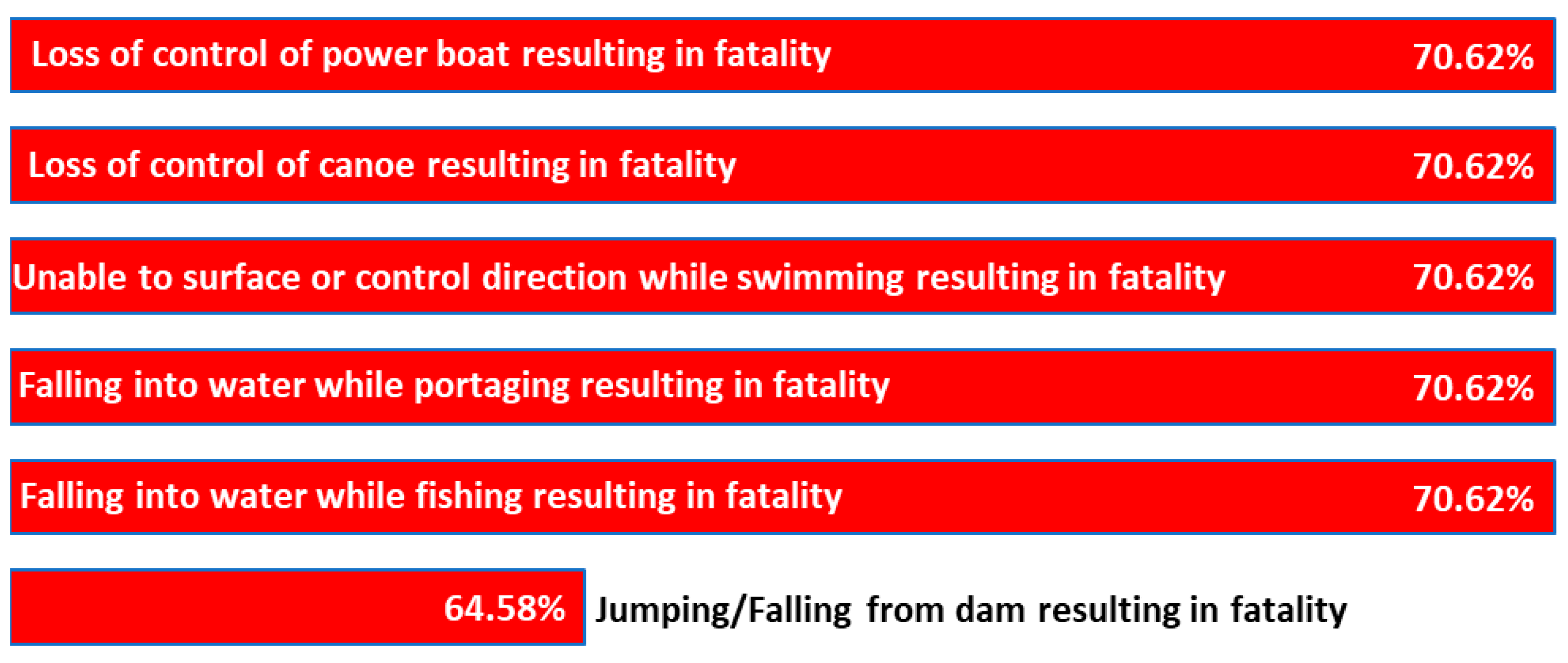
Once the individual consequences of each event on each objective have been established and combined with the corresponding objective weights, the total impact of each event can be synthesized. This synthesis captures the cumulative effect of a risk event across all relevant organizational objectives and provides a single, quantitative measure of its overall severity.

This approach ensures that the resulting impact measure reflects both the magnitude of the consequences and the strategic importance of the objectives affected. Because ratio-scale data are used for both consequence and importance, the computed impacts are mathematically meaningful and comparable across events.

Figure 15 presents the aggregated event impacts based on the analysis for this case study. These values form a critical input to the subsequent step of risk estimation, where they are combined with event likelihoods to quantify risk.

3.3.8. Computing Risk Estimates

Risk for each event is computed as the product of two fundamental components: the likelihood of the event occurring and its impact on the organization’s objectives. Each of these components, in turn, is derived from more granular estimates:

• Event likelihoods are calculated as the sum product of the likelihoods of hazards and the conditional likelihoods of the event given those hazards (vulnerabilities).
• Event impacts are computed as the sum product of the event’s consequences on each objective and the relative importance (weight) of those objectives.

This synthesis produces quantitative, ratio-scale estimates of risk, enabling meaningful comparisons across events and robust support for decision-making. It is important to emphasize that each of the four underlying estimates—hazard likelihood, conditional event likelihood, event consequence, and objective importance—must be expressed on a ratio scale. Using ordinal scales, as is often done in traditional risk matrices, results in mathematically invalid risk estimates and may lead to arbitrary or misleading management decisions [25].

Table 7. Likelihood, Impact, and Risk of Events as Percentage and Monetary Value.

Risk Event	Likelihood	Impact		Risk
		Percentage	Monetary	Percentage	Monetary
[09] Falling into water while fishing resulting in fatality	57.86%	50.64%	$12.44 M	29.30%	$7.20 M
[05] Unable to surface while swimming resulting in fatality	18.15%	46.20%	$11.34 M	8.39%	$2.10 M
[03] Loss of control of canoe resulting in fatality	10.52%	50.80%	$12.47 M	5.35%	$1.31 M
[01] Loss of control of power boat resulting in fatality	1.70%	50.06%	$12.29 M	3.06%	$752 k
[11] Jumping/Falling from dam resulting in fatality	0.26%	33.81%	$8.30 M	0.09%	$21 k
[07] Falling into water while portaging resulting in fatality	0.12%	37.32%	$9.16 M	0.05%	$11 k
Total Risk				46.23%	$11.35 M

summarizes the resulting event risks for the case study site, expressed both as percentages and as monetary values. The monetary estimates are obtained by applying a Value of Preventing a Fatality (VPF), a proxy for society’s willingness to pay for risk reduction. This approach enhances the interpretability of the results and facilitates cost–benefit analysis of risk treatment options.

3.3.9. Monetary Representation of Risk

Expressing risk in monetary terms can significantly enhance the clarity and utility of risk evaluation results by linking them directly to decision-making processes such as cost–benefit analysis, prioritization of mitigation measures, and investment justification. Because the importance of objectives in this framework is derived on a ratio scale, the total risk associated with each event can be converted into a monetary value by assigning a Value of a Prevented Fatality (VPF) to the consequences.

The VPF represents the societal willingness to pay for reducing the probability of fatality and is widely used in regulatory and policy contexts. It is not intended to reflect the value of an individual life in legal or ethical terms but rather serves as an economic indicator to support consistent decision-making.

Table 8. Reported VPF Values for Canadian Jurisdictions.

Jurisdiction	VPF Amount (Million)	In Today’s Dollars (Million)
Treasury Board of Canada Secretariat—2007 [27]	$6.11	$7.573
Transport Canada—1991 [28]	$1.5	$2.50
Policy Research Initiative—2007 [26]	$3.5–$9.5	$11.69

summarizes reported VPF estimates from Canadian jurisdictions. In this study, the upper-end estimate reported by the Policy Research Initiative [26], equivalent to $11.69 million in current dollars, is adopted.

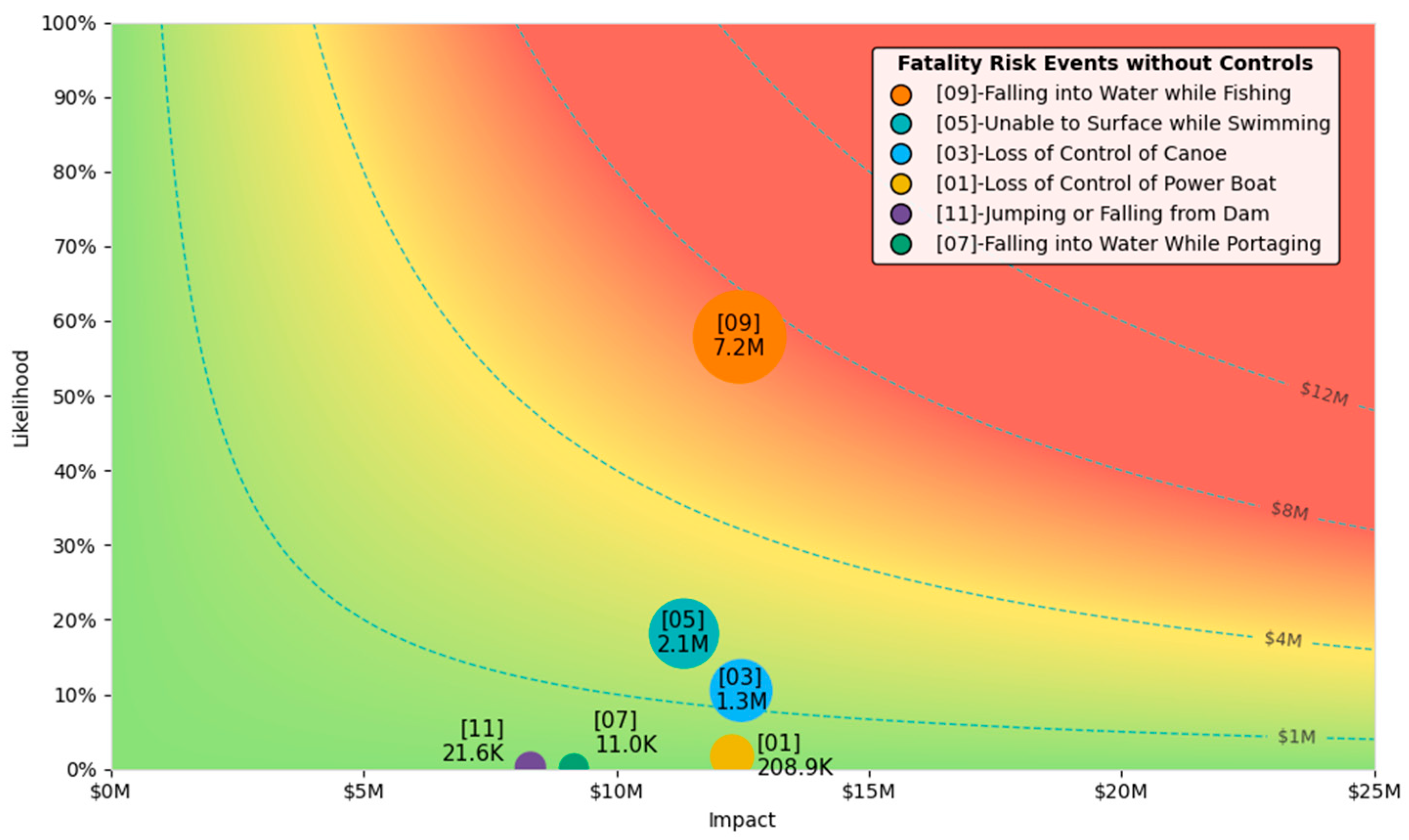
This translation enables a direct comparison between the expected risk and the potential cost of mitigation measures. For example, the total estimated risk across all events in the case study dam site over a ten-year period is approximately $11.35 million. This figure represents the expected monetary loss associated with public safety risks and provides a clear benchmark against which to assess the cost-effectiveness of control strategies. It also supports a more transparent discussion of risk treatment priorities by allowing decision-makers to evaluate whether proposed mitigation investments are justified relative to the magnitude of the risk they aim to reduce.

The spatial distribution of risk is visualized in Figure 16, where each event is represented by its likelihood (y-axis) and impact (x-axis), with bubble size proportional to overall risk. This representation helps identify which events warrant the greatest attention in risk treatment planning.

3.3.10. Bowtie Diagram with Estimates

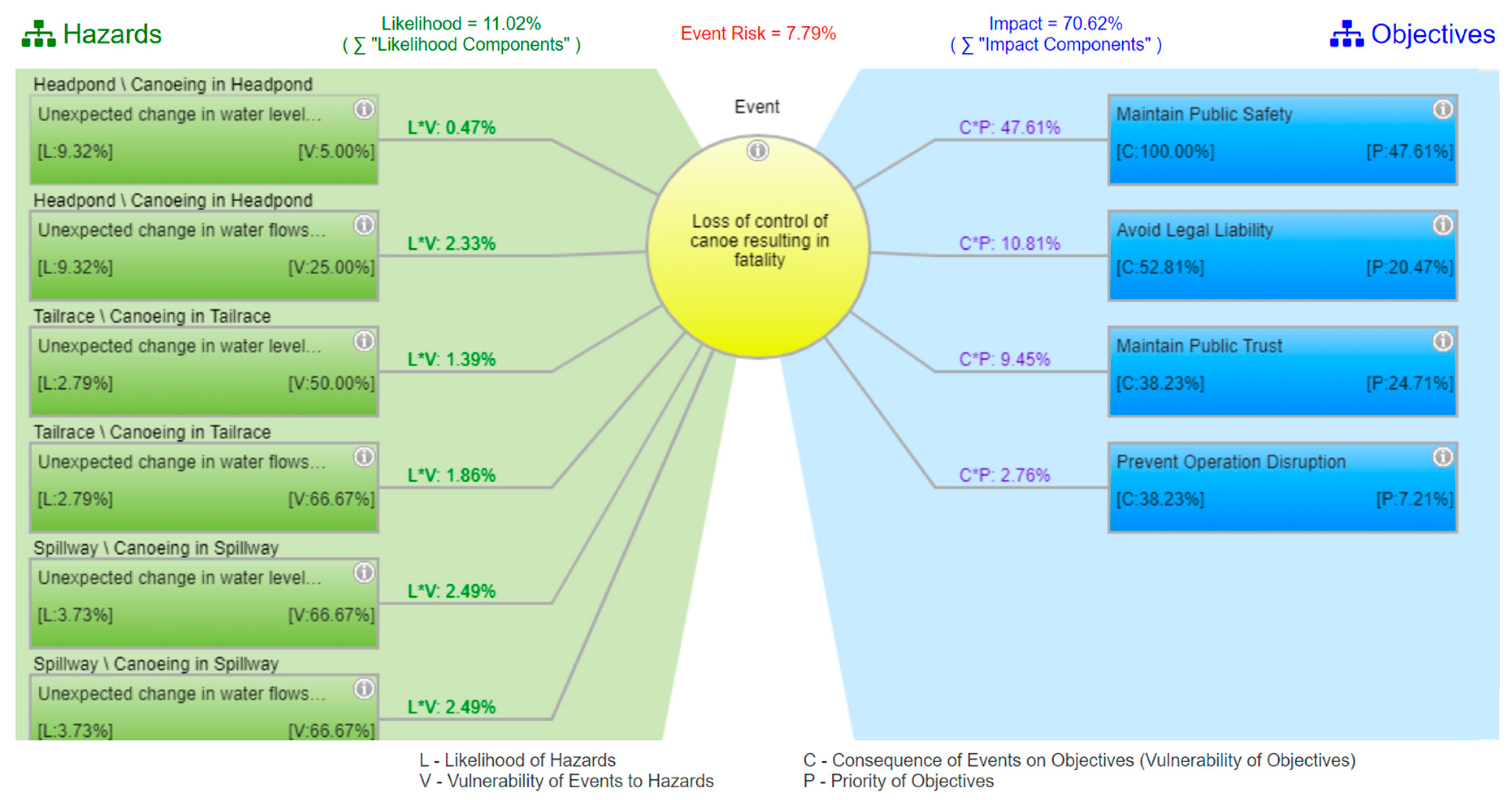
A bowtie diagram provides an integrated visualization of the relationships among hazards, events, objectives, and their quantitative measures. It connects the elements estimated throughout the analysis, including hazard likelihoods, event vulnerabilities (conditional likelihoods), consequences, objective importance, and the resulting event risk. Each bowtie diagram is centered on a specific risk event, with causes represented on the left side and consequences on the right.

Figure 17 illustrates this for the example event “Loss of control of a canoe resulting in fatality.” On the left, the hazard “canoeing in the headpond during an unexpected change in water level” has an estimated likelihood of 9.32 percent. The vulnerability of this event to that hazard is 5 percent, resulting in a contribution of 0.47 percent to the event likelihood. Summing the contributions from all applicable hazards yields a total event likelihood of 11.02 percent.

On the right side of the bowtie, the consequence of this event on the objective “Maintain Public Safety” is 100 percent. When multiplied by the priority of that objective (47.61 percent), the resulting impact is 47.61 percent of the organization’s total objective value. Adding the impacts across all affected objectives gives a total event impact of 70.62 percent. Multiplying this impact by the event likelihood produces an estimated event risk of 7.79 percent.

This visualization not only illustrates how risk is computed from its component parts but also shows how different elements of the risk framework interact in a structured and traceable way.

3.4. Simulation Outputs

3.4.1. Monte Carlo Simulation Framework

Monte Carlo simulation was applied to capture the full distribution of possible risk outcomes and address the non-linear interactions between hazards, events, and objectives that are not adequately represented through deterministic calculations. The simulations were conducted using the Riskion^® (version 6.19) platform, which integrates the computed likelihoods, vulnerabilities, consequences, and objective priorities developed in earlier stages of the analysis.

Each simulation trial represents a possible realization of system behavior over a 10-year operational period, incorporating uncertainty in hazard occurrence, event triggering, and resulting impacts. Random sampling from probability distributions was used to determine whether individual hazards occur, whether associated events are triggered, and what consequences follow for each organizational objective.

A large number of trials (typically >10,000) was performed to ensure statistical robustness. This allows the model to represent a wide range of plausible scenarios, from periods with no hazardous events to those involving severe incidents and high-consequence outcomes. Crucially, the simulation also accounts for non-linear effects, such as:

• Events triggered by multiple causes are counted only once, avoiding overestimation.
• Sequential impacts on objectives are compounded rather than summed, reflecting diminishing residual value after prior losses.

This simulation-based approach enables a more complete representation of risk by providing not just expected values but the entire distribution of possible outcomes—a necessary foundation for the analyses that follow.

3.4.2. Simulation Results and Risk Distribution

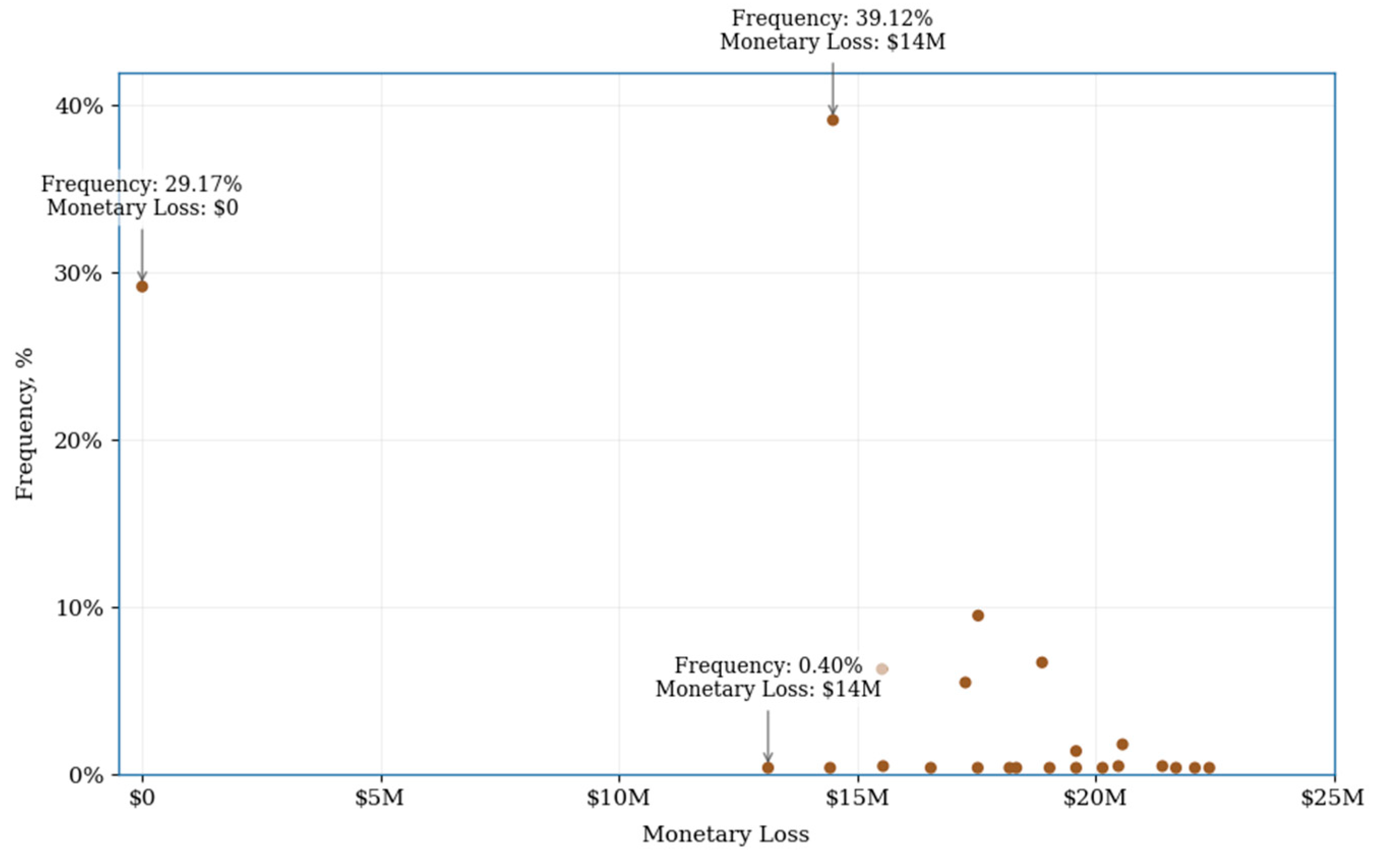
The Monte Carlo simulation produced a wide range of potential outcomes, reflecting the variability and uncertainty inherent in public-safety risks around dams. Each of the 10,000 trials represented a plausible 10-year operational period with randomized hazard occurrences, event triggers, and impacts on objectives.

Outcomes ranged from no losses in most runs to severe losses in rare but high-impact cases, such as sudden tailrace-level changes leading to vessel instability. In the most extreme trials, losses reached approximately $17 million, while roughly 29% of runs resulted in zero losses, highlighting the low-frequency but high-consequence nature of public-safety events.

The aggregated results are illustrated in the loss-frequency distribution (Figure 18), which captures the full spectrum of possible outcomes rather than a single expected value. These findings reinforce that public-safety risk around dams is inherently stochastic rather than deterministic—effective decision-making must therefore consider both the average risk and the probability of rare, high-consequence events.

3.4.3. Loss Exceedance Curve and Short-Term Risk Metrics

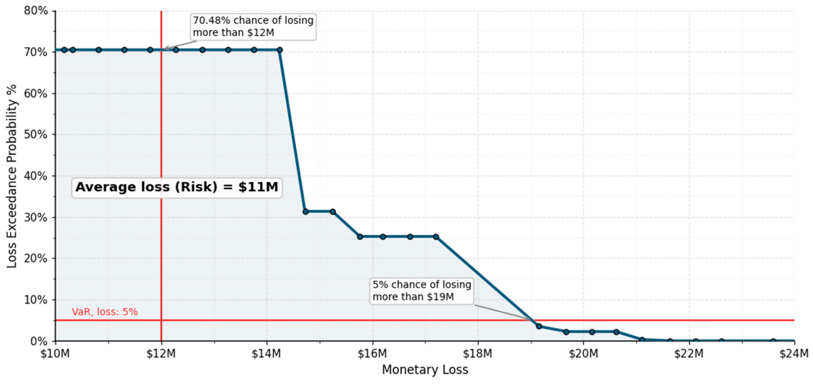
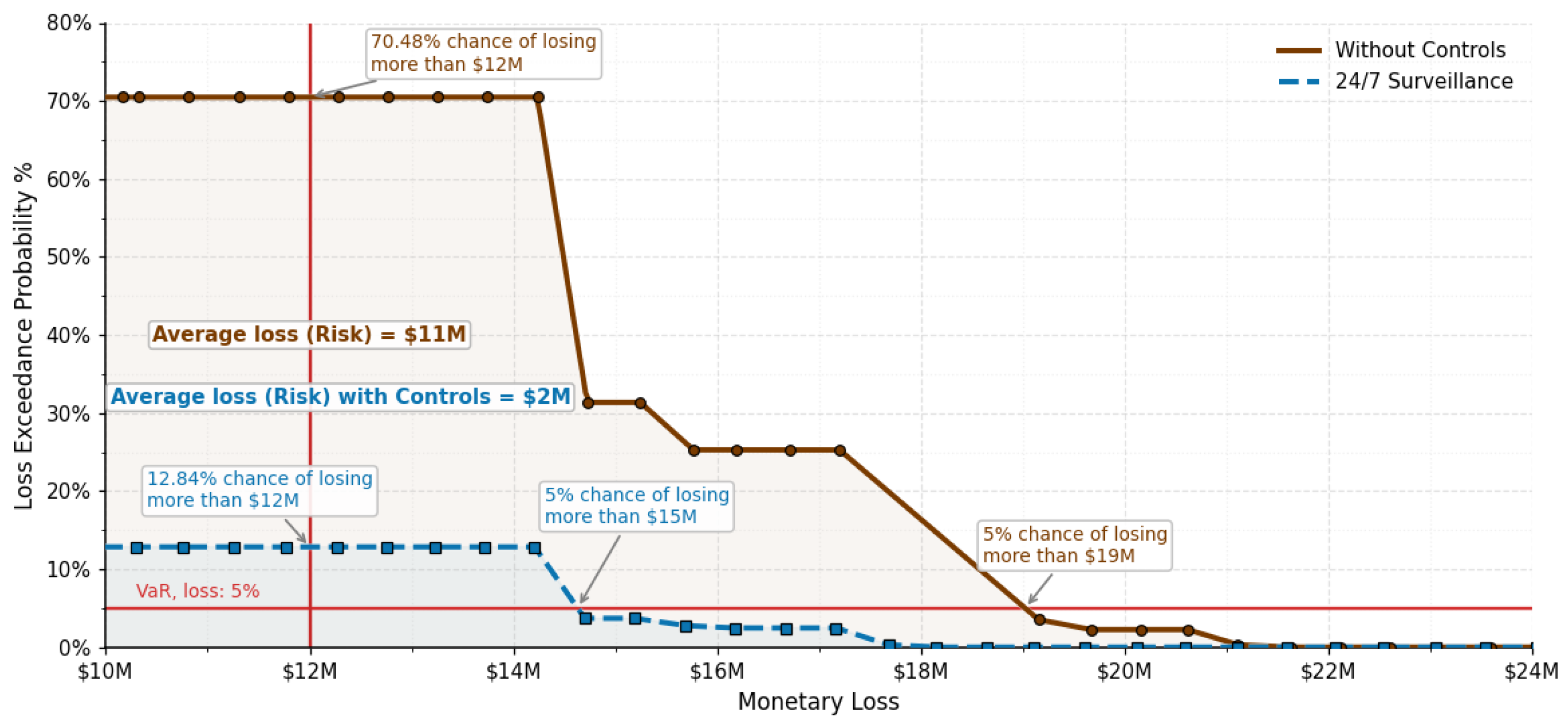
A loss exceedance curve (LEC) was developed to interpret the Monte Carlo simulation results in terms of both probability and consequence (Figure 19). The LEC expresses the likelihood that losses will exceed specific thresholds, providing a probabilistic view of potential outcomes. For instance, the analysis shows that there is less than a 5% chance that cumulative losses will exceed approximately $19.04 million over the 10-year simulation period. Similarly, the probability of experiencing losses greater than $12 million is about 70.48%.

These results are often referred to as “Value at Risk” (VaR) metrics and are widely used in risk management to quantify exposure at defined confidence levels. VaR estimates help decision-makers assess the magnitude of potential losses under rare but severe scenarios and inform the development of contingency plans and emergency response strategies.

Beyond supporting worst-case scenario planning, the exceedance probabilities also provide a practical view of short-term risk. Unlike long-term expected values, which reflect the average risk over many trials, short-term metrics capture the range and likelihood of more immediate losses that organizations may face in any given planning horizon. This probabilistic perspective enables more informed decisions about mitigation priorities, resource allocation, and acceptable levels of residual risk.

3.4.4. Long-Term Risk Behavior and the Law of Large Numbers

Monte Carlo simulation also provides insights into long-term risk dynamics. According to the law of large numbers, as the number of simulation trials increases, the average loss converges toward the expected value, which represents the system’s long-term risk profile. In this study, simulations involving thousands of trials consistently produced an expected loss of approximately $11.3 million over a 10-year period without risk controls.

This convergence indicates that while individual realizations may vary widely—with many trials producing no losses and others resulting in severe consequences—the average outcome becomes stable as the number of iterations grows. As such, the expected loss serves as a reliable measure of “steady-state” risk against which the effectiveness of future mitigation strategies can be evaluated.

Understanding this long-term behavior is critical for strategic planning. It informs investment decisions, policy development, and risk tolerance thresholds by highlighting the underlying baseline exposure of the system, even as short-term outcomes fluctuate around that average.

3.5. Treatment and Optimization Outcomes

3.5.1. Control Framework and Taxonomy

As described in Section 2.5, controls act at three stages of the risk pathway—likelihood, vulnerability, and consequence.

For the case-study dam, specific control measures were identified within each category based on site conditions, prior hazard assessments, and industry practice.

Each control was assigned an expected effectiveness distribution, cost estimate, and number of applications for modeling within the probabilistic framework.

The number of applications indicates the total count of hazard–event–objective combinations in which each control exerts influence within the simulation model, reflecting the breadth of its effect across the risk network rather than the number of physical installations.

The controls analyzed for the dam site are summarized in

Table 9. Taxonomy of control measures, targeted risk-pathway components, and modeled applications.

Control Name	Risk Pathway Target (H, V, C)	Applications
Headpond Boom	H-C	14
Headpond Fence	H-C	10
Headpond Signage	H-C	10
Tailrace Boom	H-C	10
Tailrace Fence	H-C	10
Tailrace Signage	H-C	10
Spillway Boom	H-C	10
Spillway Fence	H-C	10
Spillway Signage	H-C	10
24/7 Video Surveillance	V	81
Audible Danger Signaling Devices	H-C-V	73
Operational Controls	V-C	75
Public Education	H-C	23
Security Patrols	H-C	53
Dam Structure Fence	H-C	2

H = Hazard likelihood; V = Event vulnerability; C = Consequence Severity.

, which links each measure to its corresponding point of influence within the risk pathway and indicates the number of applications.

This applied taxonomy builds directly upon the generic control functions summarized earlier in Table 1.

3.5.2. Effectiveness Representation

Effectiveness represents the proportional reduction in hazard likelihood, event vulnerability, or consequence severity achieved when a control is implemented.

In this case study, effectiveness estimates were derived mainly from expert judgment, supported by operational experience and precedent data from comparable facilities. This approach captured site-specific factors such as public behavior, accessibility of hazardous areas, and the reliability of installed systems. Uncertainty in field performance—due to weather, user response, or system reliability—was represented through probability ranges.

To illustrate how these estimates were developed,

Table 10. Effectiveness of Headpond Boom in Reducing Likelihood of Hazards.

Target Hazard	Effectiveness	Comment
Boating Under Power	0.6	Reduces the number of powered boats entering the headpond; accounts for boom failures.
Floating debris/Power Boating	0.3	Reduces debris intrusion into the headpond, lowering risk to boats already inside.
Canoeing	0.4	Reduces canoer access; less effective than for motorboats due to ease of bypassing by land.
Floating debris/Canoeing	0.3	Similar rationale as above.
Swimming	0.4	Reduces swimmer entry; bypass possible from land without fencing.
Floating debris/Swimming	0.1	Minimal influence; bypass easy without fence.
Fishing from land	0	No effect on shore-based activity.

provides an example for boom controls installed in the headpond, spillway, and tailrace zones. These parameters were used to model reductions in the likelihood of public exposure to hydraulic hazards.

3.5.3. Standalone Risk Reduction

Each control was first evaluated individually to quantify its stand-alone risk reduction—the change in total simulated risk produced by implementing that control alone, without interaction effects.

This provides an intuitive measure of each option’s intrinsic value and a benchmark for later portfolio analysis.

Table 11. Control portfolio showing cost, number of applications, and stand-alone risk reduction.

Control Name	Cost [k $]	Stand-Alone Risk Reduction [k $]
Headpond Boom	1000	403
Headpond Fence	200	878
Headpond Signage	5	425
Tailrace Boom	500	439
Tailrace Fence	200	695
Tailrace Signage	5	76
Spillway Boom	500	715
Spillway Fence	100	828
Spillway Signage	1	152
24/7 Video Surveillance	30	9312
Audible Danger Signaling Devices	50	8966
Operational Controls	10	9027
Public Education	50	356
Security Patrols	100	3500
Dam Structure Fence	50	12

summarizes implementation cost, number of applications, and stand-alone risk reductions. Results show marked variation in performance.

Operational and monitoring controls achieved the largest absolute reductions at minimal cost.

For example, 24/7 video surveillance reduced total risk by about $9.3 million for a $30 k investment, and operational controls by $9.0 million for $10 k—both with benefit-to-cost ratios > 200:1.

By contrast, physical barriers such as headpond and tailrace booms offered limited incremental benefit relative to cost, each reducing risk by less than $1 million despite costs of $0.5–1.0 million.

Awareness and behavioral measures (e.g., signage, public education) showed moderate but cost-effective performance, with ratios typically between 10:1 and 150:1.

Overall, all control types contribute to risk reduction, but the magnitude varies widely, reinforcing the value of an optimization-based approach rather than ad hoc selection.

3.5.4. Selecting All Controls

To establish a benchmark for the upper bound of achievable risk reduction, a scenario was simulated in which all available controls were implemented simultaneously. The combined portfolio reduced total simulated risk from $11.35 million to $20,600, an overall reduction of approximately $11.33 million, at a total cost of $2.8 million, as summarized in

Table 12. Cumulative risk reduction and cost for implementation of all controls.

Scenario	Cost (k $)	Risk Reduction (k $)	Residual Risk (% of Baseline)
All Controls Implemented	2800	11,330	0.2%

.

While this represents the theoretical maximum reduction under the modeled conditions, it is neither practical nor economically justified for most dam owners. The results (Table 12) confirm diminishing returns beyond a certain investment level. Accordingly, subsequent analyses focus on cost-efficient and optimized portfolios capable of achieving comparable reductions at a fraction of the cost.

3.5.5. Selecting Typical Controls

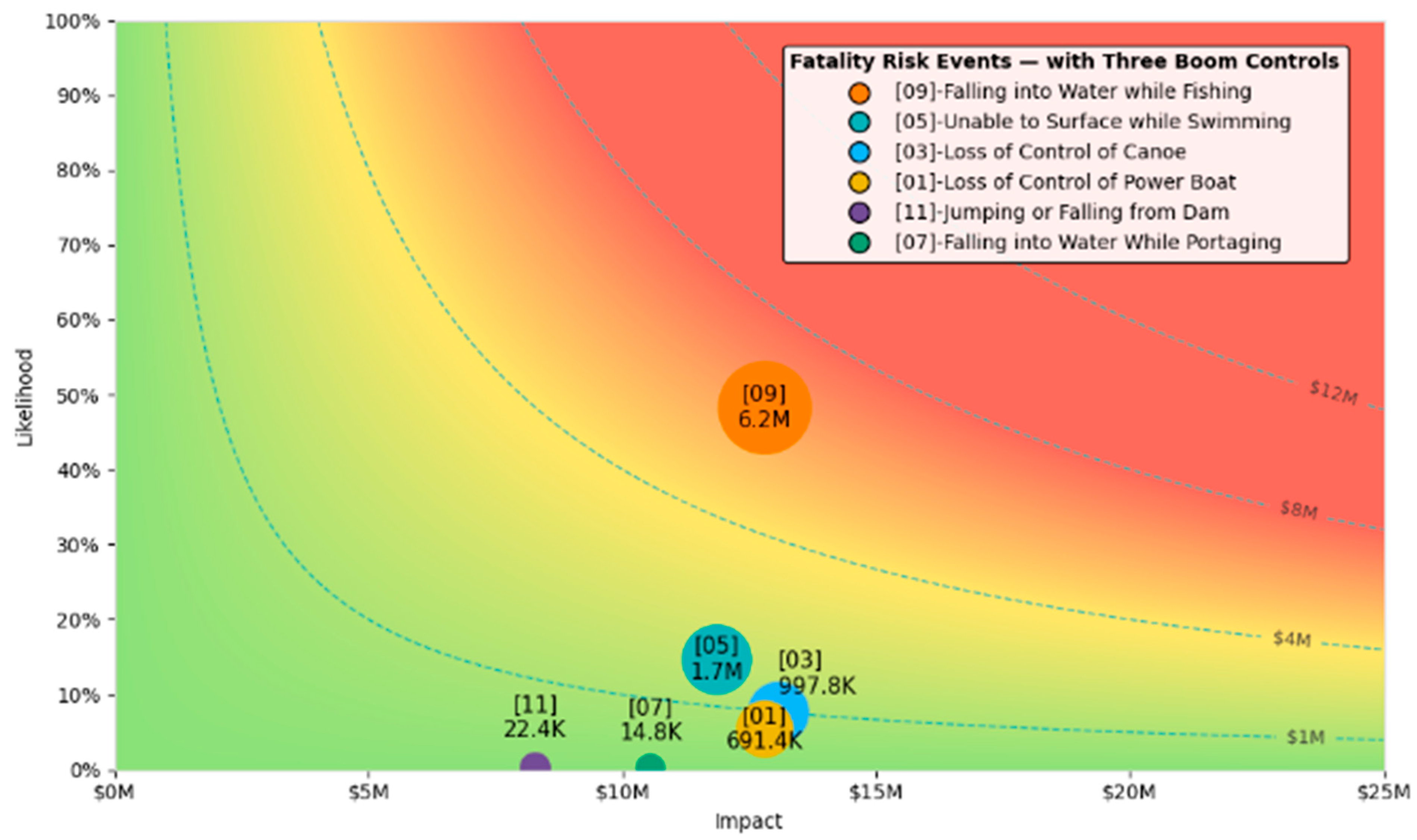
A scenario representing common industry practice—installation of three physical booms at the headpond, tailrace, and spillway—was simulated to assess the effectiveness of traditional barrier-only strategies.

As summarized in

Table 13. Risk reduction with three selected boom controls.

Scenario	Cost (k $)	Risk Reduction (k $)	Residual Risk (% of Baseline)
Three Booms Implemented	2000	1600	85.8%

, this configuration reduced total simulated risk from $11.24 million to $9.64 million, yielding a net reduction of $1.6 million for an investment of $2.0 million.

The resulting investment leverage (0.8) indicates that the achieved benefit is smaller than the expenditure, suggesting low cost-effectiveness when such measures are applied in isolation.

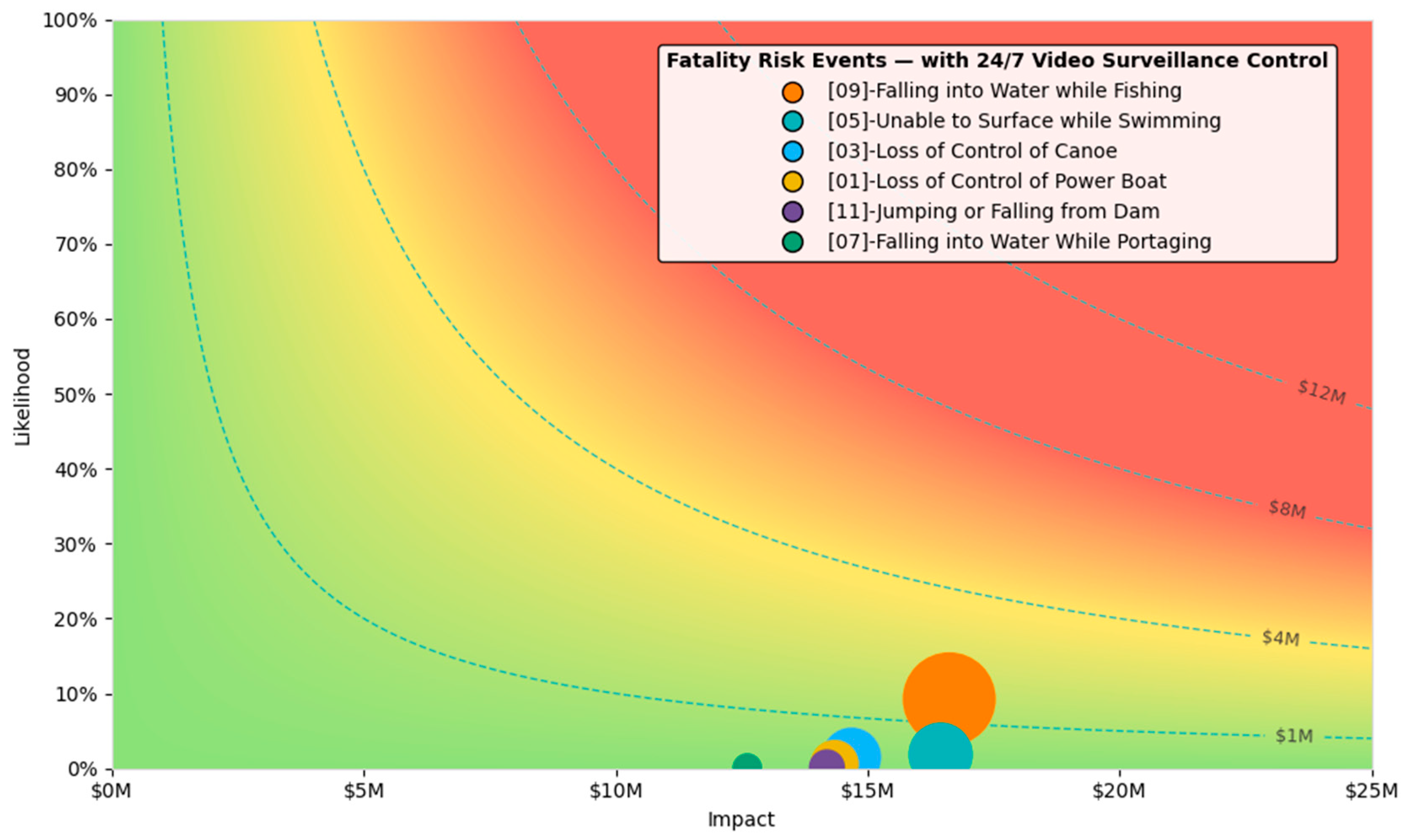
Risk heat maps (Figure 20) show minimal shifts in the distribution of event risk levels, with high-consequence scenarios largely persisting.

While these findings should not be interpreted as evidence that booms are ineffective overall, they demonstrate that physical barriers alone cannot substantially alter the public-safety risk profile.

In practice, booms are often installed as part of a layered defense strategy, complemented by operational and communication controls.

3.5.6. Selecting Controls Based on Standalone Risk Reduction

A more strategic approach involves prioritizing controls with the greatest stand-alone risk reduction per dollar invested. Under this scenario, the model identified 24/7 video surveillance as the most efficient single control measure. Implementing this control alone reduced total simulated risk from $11.24 million to $1.94 million—a reduction of $9.30 million for an investment of $30,000 (

Table 14. Risk reduction with 24/7 video surveillance control.

Scenario	Cost (k $)	Risk Reduction (k $)	Residual Risk (% of Baseline)
24/7 Video Surveillance	30	9300	17%

).

Event-specific results (Figure 21) show substantial decreases in both the likelihood and impact of fatality events, with significant compression of high-risk zones in the risk heat map. The loss-exceedance curve (Figure 22) further demonstrates a reduction in the expected average loss from $11.2 million to $1.9 million, along with notable improvement in short-term risk performance.

These outcomes highlight the dominant role of surveillance and monitoring systems in cost-effective public safety risk management. Even when applied alone, such controls can achieve reductions comparable to—or greater than—those obtained through multiple high-cost physical interventions. This insight provides a rational foundation for the optimization stage, where multiple complementary controls are combined to achieve maximum risk reduction under budgetary constraints.

3.5.7. Optimization

To identify the most cost-effective combination of interventions, a non-linear integer optimization algorithm was applied. The optimization maximized total risk reduction subject to a fixed budget constraint, explicitly accounting for overlapping and non-additive effects among controls.

Unlike the stand-alone analysis, this approach simultaneously evaluated all controls, ensuring that redundant or weakly interacting measures were not over-represented in the final portfolio.

For an assumed budget limit of $50,000, the optimization selected four controls—headpond signage, spillway signage, 24/7 video surveillance, and operational controls—as the optimum set (

Table 15. Optimum set of controls under a 50 k budget limit.

Scenario	Cost (k $)	Risk Reduction (k $)	Residual Risk (% of Baseline)
Optimized Portfolio (4 Controls)	50	11,000	2%

).

Together, these measures reduced total simulated risk from $11.24 million to $239,900, achieving a total risk reduction of approximately $11.0 million within the available budget.

This corresponds to a benefit-to-cost ratio of ~226:1.

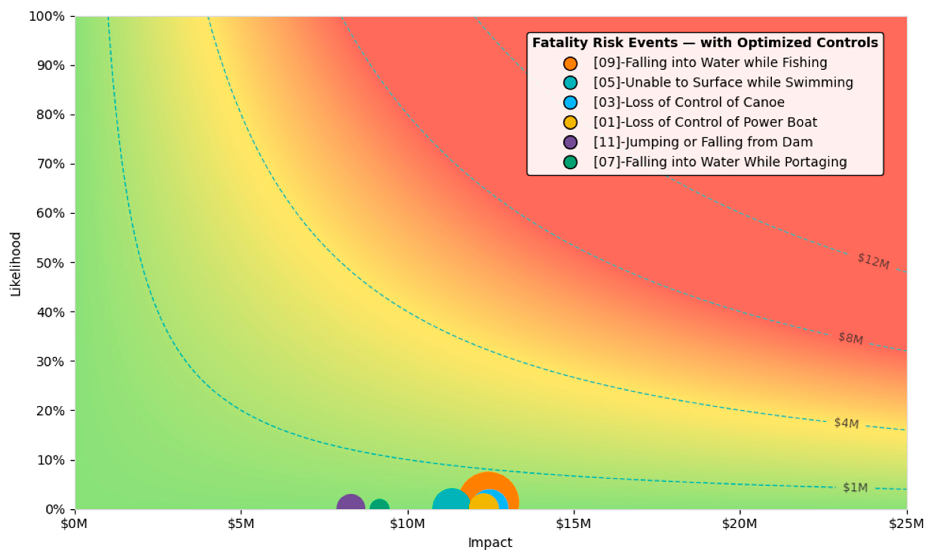
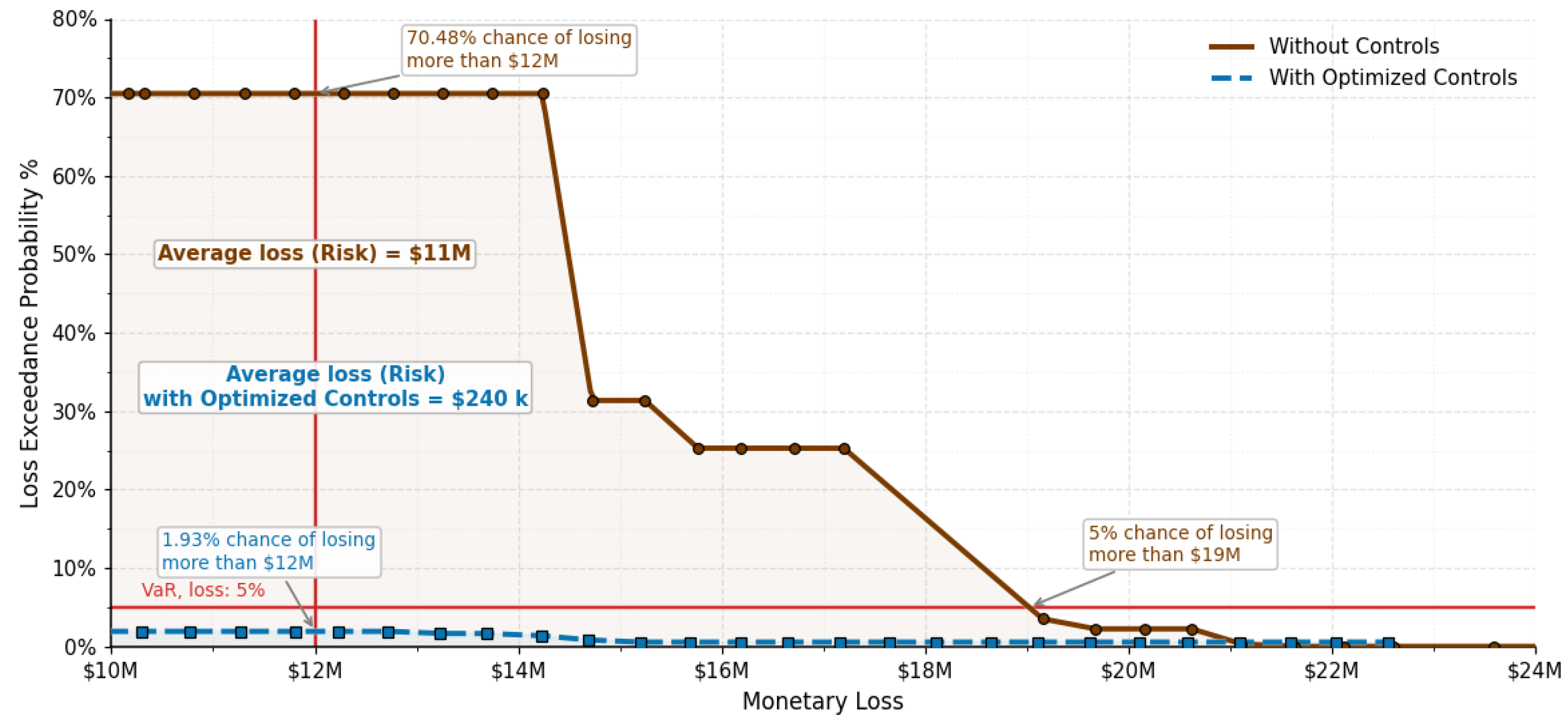
The corresponding risk heat maps (Figure 23) show a marked compression of high-risk zones across all event categories, while the loss-exceedance curve (Figure 24) illustrates a drop in mean loss from $11.4 million to $0.24 million, with the Value-at-Risk (VaR) at the 95th percentile effectively eliminated.

These findings demonstrate that the optimization algorithm consistently identifies low-cost, high-impact interventions, confirming that the most effective portfolio integrates informational, procedural, and monitoring controls rather than relying solely on physical infrastructure.

3.5.8. Efficient Frontier Analysis

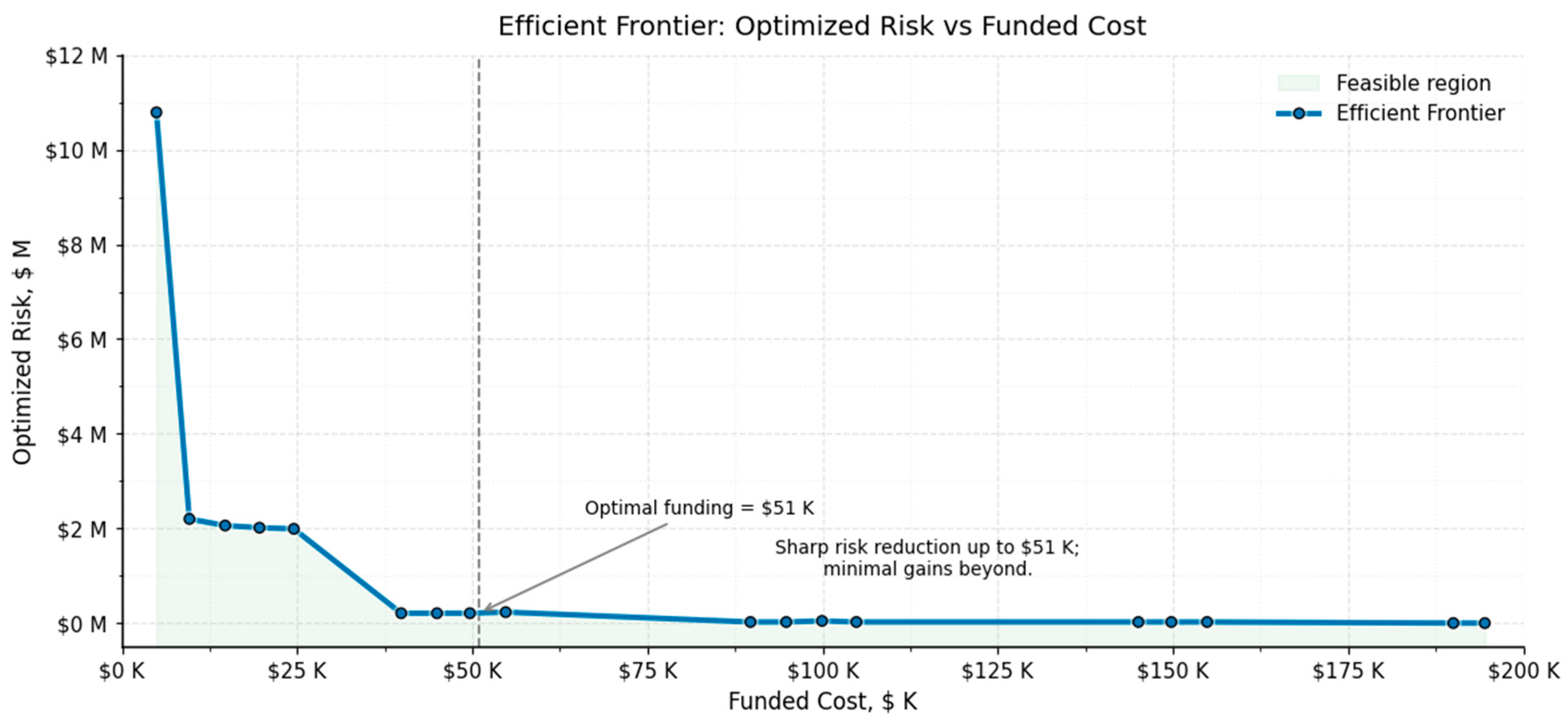
To explore the trade-off between investment and risk reduction, the optimization was repeated across a range of budget limits to construct an efficient frontier (Figure 25).

Each point on the curve represents the optimal control portfolio achieving the greatest simulated risk reduction for a given expenditure.

At low budgets, only a single control can be implemented.

For a $5000 budget, headpond signage alone is selected, providing a $0.43 million risk reduction (benefit-to-cost ≈ 86:1) but leaving residual risk above $11 million and a 68% probability of losses exceeding $12 million.

Increasing the budget to $10,000–15,000 allows operational controls, reducing total risk by about $9 million and lowering the short-term probability of major losses to below 2%.

Beyond $40,000, further spending yields little improvement, marking the onset of risk-mitigation saturation where incremental investment provides negligible benefit.

Table 16. Risk Reduction and Control Funding under Increasing Budget Scenarios. The downward arrow (↓) denotes reduction in risk.

Metric	$5 k	$11 k	$15 k	$21 k	$25 k	$41 k	$45 k	$51 k	$55 k	$91 k
Risk ↓ ($M$)	0.43	9.02	9.16	9.21	9.24	11.00	11.00	11.01	11.01	11.18
Cost ($k$)	5	10	15	20	25	40	45	50	55	90
Savings ($M$)	0.43	9.02	9.14	9.18	9.21	10.95	10.95	10.95	10.95	11.09
Leverage	86:1	902:1	610:1	460:1	369:1	275:1	244:1	220:1	200:1	124:1
Risk (Ctrl) ($M$)	11	2	2	2	2	0.3	0.2	0.2	0.2	0.1
5% Exceed. ($M$)	19	15	15	15	15
P(L > $12 M)	68%	15%	14%	14%	14%	2%	2%	2%	2%	0.4%
Headpond Boom
Headpond Fence
Headpond Signage	FUNDED		FUNDED	FUNDED	FUNDED		FUNDED	FUNDED	FUNDED
Tailrace Boom
Tailrace Fence
Tailrace Signage					FUNDED				FUNDED
Spillway Boom
Spillway Fence
Spillway Signage				FUNDED	FUNDED			FUNDED	FUNDED
24/7 Video Surveillance						FUNDED	FUNDED	FUNDED	FUNDED	FUNDED
Audible Danger Signaling Devices										FUNDED
Operational Controls		FUNDED	FUNDED	FUNDED	FUNDED	FUNDED	FUNDED	FUNDED	FUNDED	FUNDED
Public Education
Security Patrols

summarizes the optimized portfolios and performance metrics.

The efficient frontier (Figure 25) shows that over 95% of the maximum achievable risk reduction can be obtained with under 2% of the total “all-controls” cost, revealing the highly non-linear relationship between investment and residual risk.

These results provide a quantitative basis for risk-informed investment decisions, helping dam owners and regulators balance cost, performance, and safety.

The frontier visualization also clarifies how incremental funding progressively lowers residual risk, supporting transparent prioritization of future safety upgrades.

The case study demonstrates how the proposed framework integrates hazard likelihoods, event vulnerabilities, and consequence impacts into a single probabilistic representation of public-safety risk. By combining simulation and optimization, it quantifies how individual and grouped controls influence overall outcomes, revealing the non-linear relationship between cost and risk reduction. Collectively, these results show that substantial improvements in safety can be achieved through targeted, cost-efficient interventions rather than broad infrastructure expansion. The following section discusses the implications of these findings for decision-making, policy development, and the broader adoption of risk-informed dam-safety management.

4. Discussion and Future Work

4.1. Interpretation of Results

The probabilistic and optimization analyses demonstrate that public-safety risk management around dams can be strengthened through a structured, data-driven approach. The framework quantifies how different controls—ranging from physical barriers to operational procedures—affect the overall risk distribution, enabling prioritization of measures that deliver the highest benefit per cost.

Operational and information-based controls, such as surveillance, signage, and procedural measures, provide disproportionately high returns relative to their cost.

The diminishing returns observed beyond a certain investment threshold highlight the importance of optimization and cost-effectiveness analysis. Rather than pursuing maximum coverage, dam owners can focus on achieving the greatest marginal risk reduction—consistent with the ALARP principle (As Low As Reasonably Practicable).

The efficient frontier (Figure 25) illustrates this trade-off between total investment and residual risk, showing that over 95% of total achievable risk reduction can be realized within the first $50,000 of investment. Beyond this, additional spending yields minimal benefit. This quantitative insight provides a defensible basis for linking cost, control performance, and safety outcomes within a transparent decision-support framework.

4.2. Societal Risk Perspective (F-N Analysis)

While the preceding analysis optimized controls at the facility level, an equally important consideration is how those results translate into societal risk—the probability that one or more fatalities could occur across all exposure scenarios. Societal risk reflects the collective exposure of the public around a dam and provides a benchmark for determining whether overall safety performance is tolerable.

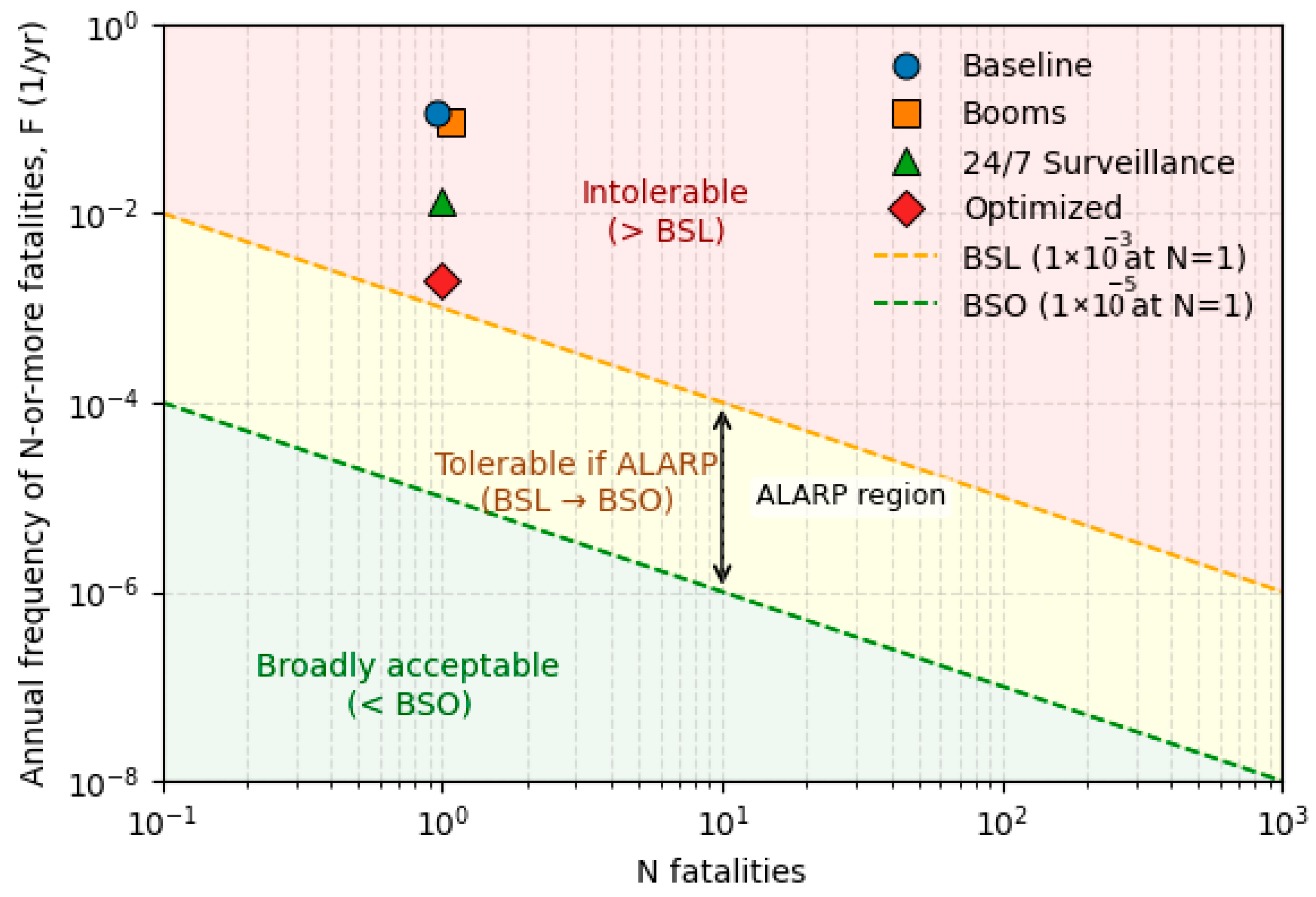
The F–N chart (Figure 26) plots the cumulative frequency (F) of events causing N or more fatalities on a log–log scale, offering a visual representation of both likelihood and consequence. In this study, societal risk was derived from the probabilistic simulation by aggregating the annual frequencies of all modeled events exceeding each fatality threshold—converted from the 10-year event probabilities used in the model. This approach converts individual event probabilities into an integrated frequency–consequence distribution, allowing comparison against the Basic Safety Objective (BSO) and Basic Safety Limit (BSL), which delineate broadly acceptable and intolerable risk regions.

These tolerability criteria align with frameworks established by the UK Health and Safety Executive [29] and adopted by the U.S. Bureau of Reclamation [30] in its Public Protection Guidelines. Within dam-safety practice, the USBR employs F–N analysis to evaluate whether residual life-safety risks—stemming from dam failure or operational incidents—fall within accepted tolerability regions. Applying the same logic here situates public-safety control evaluation within an internationally recognized governance framework.

As shown in Figure 26, pre-treatment results exceed the BSO and approach the BSL, indicating that the initial level of public protection would not satisfy common tolerability thresholds. After implementing the optimized control portfolio, the post-treatment points shift markedly downward, reflecting a substantial reduction in cumulative risk frequency and a clear movement toward the ALARP region.

By situating results within the F–N framework, the analysis connects quantitative modeling with regulatory decision-making. It provides dam owners and regulators with a visual, defensible means of communicating progress toward tolerable-risk objectives and reinforces how probabilistic methods can strengthen public-safety governance in alignment with international standards.

4.3. Reconciling Efficient Frontier and F–N Criteria

The optimized portfolios were selected to minimize expected loss, which saturates near $50,000 on the efficient frontier. The F–N criterion, however, evaluates fatal-event frequency. Because controls that reduce expected loss are not always those that most effectively lower F(N ≥ 1), the post-optimization F–N point remains slightly above the BSL at N = 1. This divergence indicates that a small number of residual exposure pathways continue to drive fatal-event frequency despite limited influence on expected loss. Two avenues are available: (i) implement targeted, low-cost measures specifically aimed at reducing F(N ≥ 1) (e.g., point-of-decision warnings, time-bound operational restrictions, micro-barriers at key approaches, focused patrol windows), or (ii) provide an ALARP justification that additional measures would be grossly disproportionate to the marginal safety improvement implied by the efficient frontier’s plateau.

4.4. Comparison with Existing Practices

Public safety risks around dams have traditionally been assessed using qualitative tools such as expert judgment, categorical matrices, and uniform application of measures like booms, fences, and signage. While useful for hazard identification, these methods offer limited insight into how specific controls influence overall risk or investment outcomes.

The proposed framework introduces a quantitative, simulation-based approach that links control performance directly to reductions in total risk and uses loss exceedance curves (LECs) and value-at-risk (VaR) metrics to express both average and extreme outcomes. This enables transparent prioritization, uncertainty evaluation, and benefit–cost analysis.

It also represents the first application of societal-risk analysis to public-safety hazards around dams, whereas past F–N evaluations have focused almost exclusively on fatalities from dam failure. The framework therefore provides both a micro-level view, optimizing controls and costs at the facility, and a macro-level view, situating results within a societal-risk and policy context.

This performance-based perspective aligns with modern asset-management and governance principles, supporting transparent, defensible, and proportionate public-safety investment decisions.

This distinction between minimizing expected loss and meeting frequency-based tolerability criteria underscores the value of multi-objective decision-making, where portfolios are screened for cost efficiency and constrained to satisfy F–N thresholds.

4.5. Practical Implementation Considerations

Operationalizing the proposed framework within a dam owner’s organization requires coordination between technical analysis, governance processes, and organizational culture. Implementation depends less on computational sophistication than on embedding a transparent, evidence-based way of reasoning within existing public-safety management systems.

The use of the Riskion^® (version 6.19) platform facilitates this process by automating expert-judgment elicitation, Monte Carlo simulation, and visualization of outcomes. This allows analysts to focus on interpretation and discussion rather than coding or statistical analysis, while maintaining traceability of assumptions and results to meet regulatory and audit expectations.

Successful integration depends on several enabling conditions:

• Data infrastructure: consistent datasets on incidents, public use, and environmental conditions to calibrate hazard likelihoods and consequence models.
• Cross-disciplinary collaboration: participation of engineers, operators, communicators, and data specialists to establish realistic control-effectiveness values.
• Change management: fostering acceptance of probabilistic reasoning and open discussion of trade-offs within planning and budgeting cycles.

Pilot applications across representative facilities can provide valuable feedback on parameter ranges, analytical procedures, and communication strategies.

4.6. Strengths and Limitations

This study presents a quantitative framework for public-safety risk management around dams, integrating AHP weighting, probabilistic simulation, and optimization into a unified decision-support process. The approach links hazard likelihoods, event vulnerabilities, and consequence severities to monetary risk metrics such as loss exceedance and value-at-risk, providing a clear basis for comparing control performance and investment efficiency. By extending societal-risk analysis beyond dam-failure scenarios, the framework connects site-level decisions with broader tolerability objectives.

Limitations include reliance on assumed data and expert judgment, simplified treatment of inter-control interactions, and exclusion of broader objectives such as environmental and operational performance [31]. Because the case study used a hypothetical facility, further applications to real sites are needed to validate and refine parameter ranges.

Despite these constraints, the framework demonstrates the practicality of applying advanced quantitative methods to public-safety risk management and provides a transparent, reproducible foundation for evidence-based decision-making in dam safety. Future validation across real dam sites will further strengthen the framework’s practical applicability and support its integration into formal dam-safety programs.

5. Conclusions

This study introduced a quantitative framework for evaluating and managing public-safety risks around dams, combining AHP-based weighting, probabilistic simulation, and optimization into a single decision-support process. The framework quantifies how controls influence hazard likelihoods, event vulnerabilities, and consequence severities, translating these into monetary risk metrics such as loss exceedance and value-at-risk.

By extending the use of societal-risk analysis beyond dam-failure scenarios, the study provides a new way to link local, site-specific decisions with broader tolerability objectives. The framework offers both a micro-level view, optimizing control portfolios at individual facilities, and a macro-level view, situating results within internationally recognized risk-governance criteria. Together, these perspectives enable transparent and defensible prioritization of public-safety investments.

The findings highlight that a small set of low-cost, high-impact controls can deliver most of the achievable risk reduction, emphasizing the importance of evidence-based prioritization over prescriptive approaches. The probabilistic and optimization components ensure that decision-making remains grounded in uncertainty analysis, benefit–cost reasoning, and ALARP principles. The analysis also shows how cost-optimal portfolios for expected loss may require small, targeted additions to satisfy frequency-based tolerability criteria, a distinction readily handled by multi-objective screening or ALARP justification.

Future application across real dam sites will allow empirical calibration of hazard likelihoods and control-effectiveness parameters, enhancing reproducibility and confidence in the method. With continued validation, the framework can support consistent, risk-informed governance across dam portfolios and contribute to the modernization of public-safety management practices.

References

1. Tschantz, B.A.; Wright, K.R. Hidden dangers and public safety at low-head dams. J. Dam Saf. 2011, 9, 1. [Google Scholar]
2. Tschantz, B.A. Public Safety at Low-Head Dams. J. Dam Saf. 2014, 12, 4. [Google Scholar]
3. Saunders, G.J. Public Safety at Dams—A Canadian Perspective. In Proceedings of the 18th Biennial Conference of the British Dam Society: Maintaining the Safety of Our Dams and Reservoirs, Belfast, UK, 3–6 September 2014; Revelstoke Design Services Limited: Winnipeg, MB, Canada. [Google Scholar]
4. Ontario Ministry of Natural Resources and Forestry (MNRF). Public Safety for Dam Owners; Government of Ontario: Toronto, ON, Canada, 2011. Available online: https://www.ontario.ca/page/public-safety-dam-owners (accessed on 17 September 2025).
5. Canadian Dam Association (CDA). Guidelines for Public Safety Around Dams; Canadian Dam Association: Ottawa, ON, Canada, 2011. [Google Scholar]
6. Cox, L.A., Jr. What’s wrong with risk matrices? Risk Anal. 2008, 28, 497–512. [Google Scholar] [PubMed]
7. Duijm, N.J. Recommendations on the use and design of risk matrices. Saf. Sci. 2015, 76, 21–31. [Google Scholar] [CrossRef]
8. Sutherland, H.; Bissett, J.; Flin, R.; Salmon, P.M. How people understand risk matrices, and how matrix design can improve their use. Risk Anal. 2021, 41, 1617–1633. [Google Scholar] [CrossRef]
9. Forman, E.H.; Forman, H.S.; Ludden, E.A. Risks We Face and Risks We Take: Enterprise Risk Management—A New Paradigm; Draft Manuscript, 2019. Available online: https://1drv.ms/b/s!AsXoAG94zEuLisQfMoBjp0lgDV3t7w?e=ykGZpo (accessed on 17 September 2025).
10. Saaty, T.L. The Analytic Hierarchy Process: Planning, Priority Setting, Resource Allocation; McGraw-Hill: New York, NY, USA, 1980. [Google Scholar]
11. Saaty, T.L. Decision making with the analytic hierarchy process. Int. J. Serv. Sci. 2008, 1, 83–98. [Google Scholar] [CrossRef]
12. Ishizaka, A.; Labib, A. Review of the main developments in the analytic hierarchy process. Expert Syst. Appl. 2011, 38, 14336–14345. [Google Scholar] [CrossRef]
13. Salloum, T.; Alrhieh, S. Dam Safety Framework for Decision-Making and Asset Portfolio Management. In Proceedings of the 87th Annual Meeting of the International Commission on Large Dams (ICOLD), Ottawa, ON, Canada, 9–14 June 2019. [Google Scholar]
14. Salloum, T.; Alrhieh, S. Dam Safety Project Portfolio Management. In Proceedings of the 2024 Canadian Dam Association Annual Conference, Niagara Falls, ON, Canada, 22–25 September 2024. [Google Scholar]
15. Savage, S.L.; Markowitz, H.M. The Flaw of Averages: Why We Underestimate Risk in the Face of Uncertainty; Wiley: Hoboken, NJ, USA, 2009. [Google Scholar]
16. Vose, D. Risk Analysis: A Quantitative Guide, 3rd ed.; Wiley: Chichester, UK, 2008. [Google Scholar]
17. Aven, T.; Krohn, B.S. A new perspective on how to understand, assess and manage risk and the unforeseen. Reliab. Eng. Syst. Saf. 2014, 121, 1–10. [Google Scholar] [CrossRef]
18. Ang, A.H.-S.; Tang, W.H. Probability Concepts in Engineering: Emphasis on Applications to Civil and Environmental Engineering, 2nd ed.; Wiley: Hoboken, NJ, USA, 2007. [Google Scholar]
19. Helton, J.C.; Davis, F.J. Latin hypercube sampling and the propagation of uncertainty in analyses of complex systems. Reliab. Eng. Syst. Saf. 2003, 81, 23–69. [Google Scholar] [CrossRef]
20. Metropolis, N.; Ulam, S. The Monte Carlo method. J. Am. Stat. Assoc. 1949, 44, 335–341. [Google Scholar] [CrossRef] [PubMed]
21. Hammersley, J.M.; Handscomb, D.C. Monte Carlo Methods; Methuen: London, UK, 1964. [Google Scholar]
22. McCormick, N.J. Risk Analysis Under Uncertainty; Springer: Cham, Switzerland, 2016. [Google Scholar]
23. Jorion, P. Value at Risk: The New Benchmark for Managing Financial Risk, 3rd ed.; McGraw-Hill: New York, NY, USA, 2007. [Google Scholar]
24. Association of State Dam Safety Officials (ASDSO). Public Safety Hazards. Available online: https://damsafety.org/public-safety-hazards (accessed on 17 September 2025).
25. Thomas, P.; Bratvold, R.; Bickel, J. The risk of using risk matrices. SPE Econ. Manag. 2013, 6, 56–66. [Google Scholar] [CrossRef]
26. Policy Research Initiative (PRI). Economic Valuation of Mortality Risk Reduction: Review and Recommendations for Policy and Regulatory Analysis; Government of Canada: Ottawa, ON, Canada, 2009.
27. Treasury Board of Canada Secretariat (TBCS). Canadian Cost-Benefit Analysis Guide—Regulatory Proposals; Government of Canada: Ottawa, ON, Canada, 2007.
28. Transport Canada (TC). Guide to Benefit-Cost Analysis in Transport Canada; TP 11875E; Government of Canada: Ottawa, ON, Canada, 1994.
29. Health and Safety Executive (HSE). Reducing Risks, Protecting People: HSE’s Decision-Making Process; HSE Books: Norwich, UK, 2001. [Google Scholar]
30. U.S. Bureau of Reclamation (USBR). Public Protection Guidelines: A Risk Framework to Support Dam Safety Decision-Making; U.S. Department of the Interior: Denver, CO, USA, 2014.
31. Canadian Dam Association (CDA). Public Safety Controls and Their Operational/Environmental Considerations; Canadian Dam Association: Ottawa, ON, Canada, 2022. [Google Scholar]
Figure 1. Typical Hydropower Dam Components for Risk Assessment (CDA, 2011).
Civileng 07 00005 g001
Figure 2. A Bowtie Diagram Visualizing Risk Elements and Risk Measures.
Civileng 07 00005 g002
Figure 3. Influence of controls on different components of the risk pathway.
Civileng 07 00005 g003
Figure 4. Hierarchy of organizational objectives considered in the case study.
Civileng 07 00005 g004
Figure 5. Hierarchy of Organization’s Objectives.
Civileng 07 00005 g005
Figure 6. Illustration of the many-to-many relationships between hazards, risk events, and their impacts on objectives.
Civileng 07 00005 g006
Figure 7. Effect of activity and gate durations on likelihood of visible and hidden hazards.
Civileng 07 00005 g007
Figure 8. Synthesized likelihoods of unexpected changes in water level and water flow for different activity and location combinations at the case study dam site.
Civileng 07 00005 g008
Figure 9. Event vulnerability to unexpected water level and flow hazards while performing activities.
Civileng 07 00005 g009
Figure 10. Event likelihood to due to unexpected change in water level and flow hazards.
Civileng 07 00005 g010
Figure 11. Event Likelihoods.
Civileng 07 00005 g011
Figure 12. Organization Objectives and their ratio scale priorities.
Civileng 07 00005 g012
Figure 13. Consequences of events to objectives.
Civileng 07 00005 g013
Figure 14. Event impacts on objectives.
Civileng 07 00005 g014
Figure 15. Overall Event Impacts.
Civileng 07 00005 g015
Figure 16. Risk Map showing Event Risks at Damsite. Color contours are for visual guidance only and do not represent risk thresholds or acceptance criteria.
Civileng 07 00005 g016
Figure 17. Illustrative bowtie showing relative component weights within the risk pathway.
Civileng 07 00005 g017
Figure 18. Frequency Distribution of Losses.
Civileng 07 00005 g018
Figure 19. Loss Exceedance Curve.
Civileng 07 00005 g019
Figure 20. Risk Heat Maps with Three Selected Boom Controls. Color contours are for visual guidance only and do not represent risk thresholds or acceptance criteria.
Civileng 07 00005 g020
Figure 21. Risk Heat Maps with 24/7 Video Surveillance Control. Color contours are for visual guidance only and do not represent risk thresholds or acceptance criteria.
Civileng 07 00005 g021
Figure 22. Loss Exceedance Curve with the 24/7 Video Surveillance control.
Civileng 07 00005 g022
Figure 23. Risk Maps showing Event Risks after applying controls at Damsite for 10-year timeframe. Color contours are for visual guidance only and do not represent risk thresholds or acceptance criteria.
Civileng 07 00005 g023
Figure 24. Loss exceedance curve corresponding to a budget level of 50 K.
Civileng 07 00005 g024
Figure 25. Efficient Frontier of optimal portfolios of controls.
Civileng 07 00005 g025
Figure 26. F-N Chart with ALARP Regions for Public Safety Fatalities.
Civileng 07 00005 g026