Does Geographic Proximity Matter for Happiness? Spatial Panel Evidence from the European Union (2015–2024)

Abstract

This study analyzes the determinants and spatial dependence of happiness across the 27 European Union Member States during 2015–2024. It uses a panel of 270 observations based on the Cantril Ladder and the six explanatory factors from the World Happiness Report: GDP per capita, social support, healthy life expectancy, freedom, generosity, and perceptions of corruption. The empirical strategy combines panel models and spatial econometrics. Specification tests support a model with country random effects and year fixed effects. Spatial autocorrelation is assessed using Moran’s I, and random effects (RE), spatial autoregressive random effects (SAR-RE), the spatial error model with random effects (SEM-RE), and the spatial autoregressive model with spatially autocorrelated errors and random effects (SARAR-RE) are considered, using a three-nearest-neighbor matrix. The results show a strong and persistent spatial concentration of happiness. However, the non-spatial model absorbs most of this dependence, leaving no significant residual spatial autocorrelation for the full period. Consistently, neither SAR-RE nor SEM-RE significantly improves model fit, and the information criteria, likelihood-ratio tests, and Baltagi–Song–Koh tests support the non-spatial RE model with year fixed effects. GDP per capita, social support, and freedom show positive associations with happiness, while perceptions of corruption show a negative association. Healthy life expectancy and generosity are not statistically significant. Moreover, all six WHR determinants exhibit significant spatial autocorrelation, suggesting that the geographic clustering of happiness largely reflects the spatial concentration of its underlying socioeconomic, social, health, and institutional determinants rather than a direct contagion of happiness between neighboring countries. The study underscores the importance of considering the spatial dimension in wellbeing analysis and of accounting for shared regional socioeconomic and institutional conditions when designing European wellbeing policies.

1. Introduction

Interest in happiness as an essential human goal, although it dates back to classical thought, has gained increasing prominence in academic debate in recent decades [1]. One of the main reasons for this is undoubtedly the recognition that indicators such as gross domestic product cannot, by themselves, adequately represent social progress and quality of life [2]. This limitation may be especially relevant in affluent economies, where further economic expansion can generate diminishing gains in life satisfaction while continuing to increase resource and energy use, reinforcing the need to assess wellbeing directly rather than treating GDP as a sufficient proxy for social progress [3]. This concern contributed to the development of the economics of happiness, an interdisciplinary field that systematically analyzes the economic, social, and institutional determinants of subjective wellbeing [4,5].

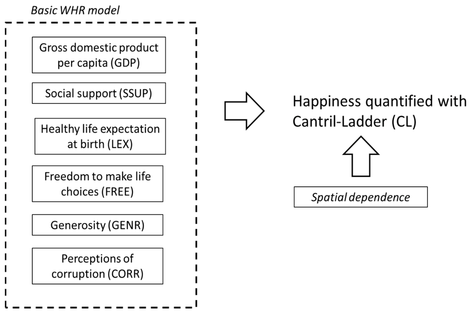
One of the main analytical frameworks for the empirical study of happiness is the framework based on the Gallup World Poll and incorporated annually into the World Happiness Report (WHR) [6]. Its main indicator is the Cantril Ladder (CL), through which individuals rate their present life on a scale ranging from 0, corresponding to the worst possible life, to 10, associated with the best possible life. Building on this overall evaluation, the WHR explanatory model relates international differences in happiness to six factors: GDP per capita, social support, healthy life expectancy, freedom to make life choices, generosity, and perceptions of corruption [6]. As summarized in Figure 1, this approach links a subjective measure of wellbeing with objective and perceptual indicators of the economic, social, and institutional environment, and helps shed light on why life evaluations differ across societies [1]. This multidimensional perspective is consistent with broader research on global issues, which increasingly emphasizes that social, political, economic, and environmental challenges are interconnected and should therefore be examined through holistic analytical frameworks [7].

The WHR model has frequently been used as a baseline specification for incorporating additional variables, thereby expanding knowledge about the factors associated with happiness [8]. However, limited attention has been paid to the spatial structure of the data in applications of the model. This omission is relevant, given that happiness levels display geographic patterns and tend to cluster in certain areas rather than being independently distributed across territories [9]. Place of residence encompasses environmental, urban, economic, and institutional conditions that may help explain part of wellbeing and substantially improve the fit of happiness functions [10]. Moreover, the relationships between the determinants of wellbeing may vary across territories, while outcomes in neighboring countries may be interrelated. Ignoring this heterogeneity and spatial dependence can affect both the efficiency of estimates and the validity of statistical inference [11]. Recent studies also document territorial clustering and spillover effects between neighboring units, reinforcing the case for applying spatial econometric techniques to the analysis of life satisfaction [12].

In light of these considerations, this study examines the determinants of happiness in the 27 Member States of the European Union (EU) over the period 2015–2024, following the framework depicted in Figure 1. The first aim is to assess which variables from the basic WHR model retain explanatory power within a supranational space characterized by a high degree of economic, political, and regulatory integration. The second is to determine whether, once these factors are accounted for, a significant spatial structure persists in happiness levels. The EU provides a particularly suitable setting for this analysis, as it combines considerable diversity among countries with a shared institutional, legal, and political framework, along with a certain degree of convergence in economic, social, and environmental dimensions [13].

Accordingly, the following research objectives are formulated:

RO1. 

To identify the WHR components associated with differences in happiness across EU countries while controlling for common temporal changes. Thus, the following hypotheses are formulated:

H1a. 

GDP per capita is positively associated with happiness across EU countries.

H1b. 

Social support is positively associated with happiness across EU countries.

H1c. 

Healthy life expectancy is positively associated with happiness across EU countries.

H1d. 

Freedom to make life choices is positively associated with happiness across EU countries.

H1e. 

Generosity is positively associated with happiness across EU countries.

H1f. 

Perceptions of corruption are negatively associated with happiness across EU countries.

RO2. 

To assess whether geographic proximity among EU Member States contributes to explaining happiness in a panel data context. Accordingly, the following hypotheses are proposed:

H2a. 

Happiness exhibits positive spatial dependence across geographically proximate EU countries.

H2b. 

Significant spatial dependence remains after controlling for the standard WHR determinants, persistent country heterogeneity, and common year effects.

The study makes two main contributions. First, the use of longitudinal data makes it possible to exploit both changes occurring within countries over time and persistent differences between countries. Second, the incorporation of spatial econometrics allows the analysis to move beyond the assumption of geographic independence and to assess whether happiness levels exhibit spatial dependence across neighboring countries. This approach helps identify not only which variables are associated with happiness, but also whether Europe’s territorial configuration contributes to explaining its geographic distribution. The novelty therefore lies not merely in documenting the well-known geographic clustering of happiness across Europe, but in testing whether this pattern persists after controlling for the standard WHR determinants, country-specific heterogeneity, and common temporal effects. Moreover, by examining the spatial distribution of the WHR determinants themselves, the study assesses whether the geography of happiness reflects an additional spatial process or largely overlaps with the geography of its underlying determinants.

The article is organized as follows. Section 2 reviews the literature on aggregate happiness based on the WHR model, and on the relevance of the territorial dimension of wellbeing. Section 3 describes the data and the quantitative analysis strategy. Section 4 presents the empirical results. Finally, Section 5 discusses the findings and sets out their main implications, and Section 6 presents the study’s conclusions and limitations.

2. Literature Review

2.1. Models Extending the WHR

A first strand of the literature reviewed consists of studies that extend the WHR model by incorporating new explanatory variables. The second comprises research that fully or partially retains the WHR structure but relies on alternative data analysis methods, such as configurational techniques or machine learning algorithms, with the aim of capturing relationships that conventional regression may represent insufficiently.

Within the first group, some studies incorporate technological, institutional, or cultural dimensions into the WHR model, such as countries’ degree of digitalization [14] or their commitment to sustainability and its interaction with institutional factors [15]. Mahalik and Harris [16] show that beliefs associated with precarious masculinity are negatively related to national happiness, both directly and through their links to structural conditions, including social support and health. Zong [17], in turn, partially challenges the traditional WHR specification by finding that generosity contributes little to explaining cross-country differences in happiness and arguing that inequality and educational conditions should receive greater attention.

Other extensions of the WHR model introduce specific macroeconomic and political variables, such as the credit cycle [18] or the degree of territorial decentralization of states [19]. Other papers shift the assessment toward organizational settings. Chen et al. [20] show that social happiness can influence corporate decisions and act as a form of “soft institution” that shapes business behavior. Pološki Vokić and Klindžić [21], in turn, examine the relationship between national-level human resource practices and aggregate wellbeing levels.

The second group of studies is not necessarily characterized by the incorporation of new determinants or theoretical frameworks, but rather by proposing analytical strategies that move beyond conventional regression, which remains dominant in this literature. These studies rethink how relationships between known variables are examined through nonlinear, configurational, predictive, or hybrid approaches [8]. Consequently, their main contribution lies not so much in expanding the model’s content as in modifying how such relationships are identified and represented—that is, less in the “what” explains happiness than in the “how” it is explained. Thus, while Tofallis [22] proposes a multiplicative respecification of the WHR model, other studies draw on fuzzy set theory, which allows for the analysis of configurational relations among explanatory conditions and happiness [23,24].

Another set of studies, also linked to the incorporation of new techniques, uses machine learning algorithms to enhance the predictive ability of WHR-based models. These applications include regularized regressions [25,26], decision trees, Random Forest, and XGBoost [25,27,28,29,30], as well as deep neural networks and graph neural networks [31]. Taken together, these approaches make it possible to identify complex patterns, interactions, and nonlinear relationships that may remain hidden in traditional econometric specifications.

2.2. Happiness and Spatial Analysis

Spatial analysis of happiness remains a relatively limited line of research within welfare economics, although prior work has employed a wide variety of methodological approaches. In this context, four strands can be distinguished.

The first strand combines the diagnosis of autocorrelation with spatial regression models. Moran’s I and a spatial error model are applied to relate national happiness to economic freedom, GDP per capita, inflation, and unemployment [9]. They observe geographic clustering of happy and unhappy countries, as well as positive effects of GDP and economic freedom and negative effects of inflation and unemployment. CL data, Moran’s I, a spatial model estimated via instrumental variables, and a Durbin model are used to study globalization, unemployment, and corruption control [32]. Their results show spatial dependence and indirect effects from neighboring countries’ conditions. Using Moran’s I, Local Indicators of Spatial Association (LISA), a spatial autoregressive model (SAR), a spatial error model (SEM), and the spatial Durbin model (SDM), life satisfaction in Canadian communities is found to depend on the satisfaction, income, and unemployment of neighboring communities, confirming the existence of territorial spillovers [12].

A second set of studies focuses not so much on contagion between territories as on testing whether the relationships between happiness and its determinants change according to location. The effects of income and unemployment on life satisfaction are first estimated for each country, and the spatial distribution of those coefficients is then analyzed [11]. Income is found to have a greater impact in less developed countries, and the subjective cost of unemployment is found to be more intense in economies with higher GDP or unemployment [11]. Geographically weighted ordinal regression is used to show that the negative effect of pollution on life satisfaction varies across areas of Beijing [33]. Using random parameters and latent class models, the valuation of pollution, crime, urbanization, and other local attributes is likewise found not to be homogeneous across Chilean municipalities [34]. These studies provide evidence of territorial heterogeneity, although they do not reproduce the WHR explanatory model and do not necessarily estimate spillover effects between neighbors.

A third category uses descriptive spatial techniques without estimating a spatial happiness function. Moran’s I is applied to educational, health, residential, and environmental variables that make up an objective wellbeing index in Argentina, showing that these dimensions display different degrees of geographic concentration [35]. Moran’s I and the Getis–Ord statistic are combined to detect hot and cold spots of Instagram posts tagged #happy, relating them to urban land use [36]. These studies help identify territorial patterns and areas of concentration, but do not determine how a change in one territory’s conditions statistically affects its own happiness or that of its neighbors.

Finally, in the fourth strand, some studies incorporate geography without resorting to spatial econometrics as such. Geographic information systems and ordinal regression are used to relate life satisfaction to income, employment, health, and education, as well as climate, urbanization, coastal proximity, and other environmental characteristics; territorial variables are concluded to substantially improve the model’s explanatory power [10]. Using descriptive analyses, linear trends, and Spearman correlations for 141 countries, a positive association is found between latitude, human development, and happiness, which is stronger in the global sample than in the European one [37].

Within this fourth strand, a regional wellbeing index is constructed using Fuzzy-Hybrid TOPSIS and quantile regression, linking it to age, education, and income [38]. Using multilevel models, the proportion of wellbeing variability corresponding to the country level versus subnational levels is quantified [39]. Taken together, this body of work confirms that place matters, but also shows that an integrated framework combining CL, the full WHR model, panel data, and spatial econometrics within a homogeneous institutional context such as the European Union is still lacking.

All of these studies depart, to varying degrees, from the basic WHR model (in which the explanatory variables are GDP per capita, social support, healthy life expectancy, freedom to make life choices, generosity, and perceptions of corruption) and rely on partial specifications tailored to their respective objectives. In this sense, this study can be situated at the intersection of the two main strands that extend the “pure” WHR model. On one hand, it explicitly incorporates the spatial dimension through spatial regression models. This extension makes it possible to consider either that a country’s happiness is related to that of geographically nearby countries, or that spatial dependence exists in the error term. In the latter case, spatial correlation would reflect the presence of common territorial factors that are unobserved or not captured by the explanatory variables included in the model [40]. On the other hand, the analysis is carried out within a clearly defined geographic, political, and institutional setting, the European Union, which makes it possible to evaluate the WHR model across a set of countries subject to a common regulatory framework and a significant degree of economic and social integration.

A first mechanism through which geographic proximity may be associated with similar levels of wellbeing concerns the persistence and geographic distribution of cultural values. Hofstede’s classic framework conceptualizes national cultures as relatively stable configurations of values that differ systematically across countries along dimensions such as individualism, power distance, uncertainty avoidance, and masculinity [41]. Subsequent research has likewise shown that modernization does not eliminate historically rooted cultural differences. Cultural change is path dependent, and religious, historical, and institutional traditions continue to leave a persistent imprint on national value systems [42]. Because neighboring European countries often share elements of historical experience, religion, institutional development, and patterns of social interaction, cultural values may themselves exhibit a territorial structure. These shared cultural environments can shape social trust, perceived autonomy, social support, attitudes toward institutions, and the way individuals evaluate their lives. Spatial clustering in happiness may consequently arise because geographically proximate countries share cultural and institutional backgrounds that influence both happiness and its observable determinants [43].

Another mechanism linking geographic proximity to similar levels of wellbeing is the territorial clustering of institutional and welfare-state arrangements. Comparative welfare-state research has long shown that European countries are not institutionally homogeneous, but tend to be grouped into relatively persistent welfare-regime families characterized by different combinations of state provision, market dependence, social protection, and family support [44]. This institutional differentiation also has a geographic component. For example, Ferrera [45] identified a distinctive Southern European welfare model shared by Italy, Spain, Portugal, and Greece, reflecting common historical and institutional traits. Such geographically clustered welfare arrangements may influence several determinants directly related to happiness, including income security, social protection, health provision, interpersonal support, and perceptions of institutional effectiveness. Geographic similarity in happiness may therefore partly reflect the spatial concentration of institutional structures rather than direct transmission of wellbeing between neighboring countries.

3. Materials and Methods

3.1. Description of the Variables

The dataset used in this study is based on the World Happiness Report (WHR), which draws on data from the Gallup World Poll [6]. The analysis covers the 27 EU Member States over the period 2015–2024, resulting in a balanced panel of 270 country-year observations.

Table 1. Descriptive statistics of the WHR variables for the period 2015–2024.

Variable	Mean	Median	SD	CV (%)	Maximum	Minimum
CL	6.51	6.46	0.66	10.15	7.86	4.84
GDP	10.62	10.58	0.36	3.41	11.81	9.9
SSUP	0.83	0.85	0.1	12.09	0.97	0.53
LEX	70.07	70.88	2.11	3.01	75.32	63.87
FREE	0.72	0.71	0.14	19.35	0.96	0.31
GENR	−0.09	−0.12	0.14	NA	0.34	−0.34
CORR	0.65	0.76	0.25	38.78	0.96	0.1

Note: SD = standard deviation, and CV is coefficient of variation. GDP corresponds to the WHR Log GDP per capita variable, whereas LEX is reported in its original level. LEX was subsequently log-transformed for model estimation.

reports the descriptive statistics. The variables are defined and measured following the WHR methodology [6].

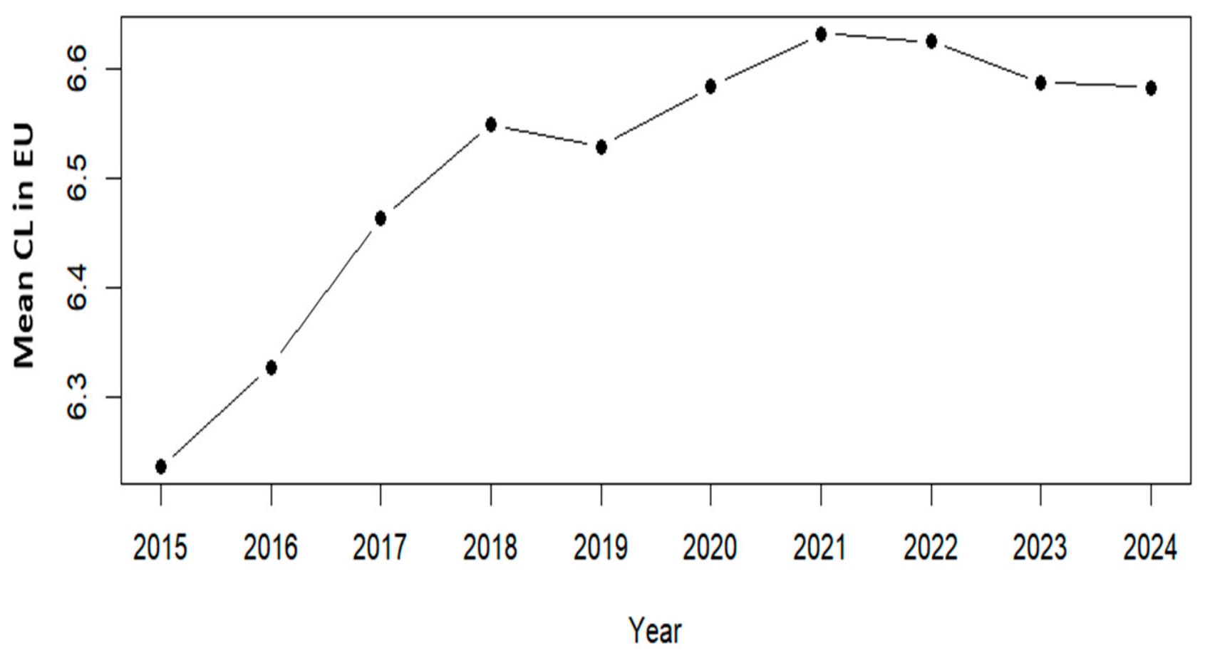
The dependent variable is happiness or subjective wellbeing, measured using the well-known Cantril Ladder (CL) scale. Specifically, individuals respond to the question, “Please imagine a ladder with steps numbered from 0 at the bottom to 10 at the top. The top of the ladder represents the best possible life for you and the bottom of the ladder represents the worst possible life for you. On which step of the ladder would you say you personally feel you stand at this time?” The variable used is the national average of these responses. The definition and measurement of the Cantril Ladder remained consistent throughout the 2015–2024 period, and the panel includes the same 27 EU Member States in each year. Figure 2 shows that over the study period, average happiness across EU countries increased gradually until 2021 and remained broadly stable thereafter.

The economic component is GDP per capita, based on World Development Indicators data and expressed in constant international dollars adjusted for purchasing power parity. When observed values for the most recent years are unavailable, the WHR series incorporates available estimates and projections. In the WHR dataset, GDP per capita is already provided in natural logarithmic form, and this variable is used directly in the empirical models without any additional logarithmic transformation.

Social support (SSUP) captures the share of respondents who indicate that they have family members or friends available to assist them in difficult circumstances. Country-level values therefore summarize the prevalence of dependable interpersonal networks within each population.

Healthy life expectancy at birth (LEX) is derived from World Health Organization statistics and reflects both expected longevity and population health conditions. Gaps in the underlying series are addressed through interpolation or extrapolation to maintain comparability over time. It is initially reported in years, but in the regression analysis its natural logarithm is used in subsequent assessments.

Freedom to make life choices (FREE) corresponds to the proportion of respondents who express satisfaction with their ability to decide how to conduct their lives. It is therefore interpreted as an aggregate indicator of perceived personal autonomy.

Generosity (GENR) is defined as the country-level residual obtained after regressing the average response to whether individuals donated money to charity during the previous month on GDP per capita. This adjustment is intended to isolate generosity from national income differences.

Perceptions of corruption (CORR) are represented by the proportion of respondents who consider corruption to be widespread in government or business. Higher values indicate weaker perceived institutional integrity and lower confidence in public and private institutions.

Based on these variables, the baseline empirical specification can be expressed as:

$${CL}_{it}=b_0+b_1{GDP}_{it}+b_2{SSUP}_{it}+b_{3}ln\left({LEX}_{it}\right)+b_4{FREE}_{it}+b_5{GEN}_{it}+b_6{CORR}_{it}+{\mu }_i+{\tau }_t+{\epsilon }_{it}$$

(1)

where ${CL}_{it}$ denotes the average CL score for country i in year t; ${GDP}_{it}$ is the Log GDP per capita variable provided directly by the WHR; ${SSUP}_{it}$ denotes social support; ${LEX}_{it}$ is healthy life expectancy, entered in the model in natural logarithmic form; ${FREE}_{it}$ represents freedom to make life choices; ${GEN}_{it}$ denotes generosity; and ${CORR}_{it}$ represents perceptions of corruption. The term ${\mu }_i$ captures time-invariant country-specific heterogeneity, ${\tau }_t$ captures common year effects, and ${\epsilon }_{it}$ is the idiosyncratic disturbance.

3.2. Data Analysis

3.2.1. Data Treatment and Panel-Data Specification

Before conducting the statistical analysis, seven missing values were imputed: two for Bulgaria, two for Croatia, and one for Romania in the CORR variable, together with two for Greece in the GENR variable. These seven values represent only 0.43% of the 1620 predictor values (270 country-year observations × 6 explanatory variables). When observations were available for both the preceding and following years, missing values were estimated by linear interpolation. When only one adjacent observation was available, the nearest available temporal value was carried forward or backward, as appropriate. No missing values were present in the dependent variable. To assess whether this limited imputation affected the results, the main model was also re-estimated after excluding the country-year observations containing imputed values.

The empirical analysis was subsequently carried out in two complementary stages. To select ex ante the most appropriate panel data model specification, a pooled model (pooled OLS), a country fixed-effects model (FE), and a country random-effects model (RE) were estimated in sequence, keeping the same set of explanatory variables across all of them [46]. In the empirical specification of CL, the WHR-provided Log GDP per capita variable was used directly, whereas healthy life expectancy (LEX), originally provided in levels, was transformed using its natural logarithm. First, the F test allowed for comparison of the pooled model with the fixed-effects model. Its null hypothesis states that the countries’ individual effects are jointly equal to zero. Second, the Breusch–Pagan Lagrange multiplier test compares the pooled model with the RE model, under the null hypothesis that the variance in the individual component is zero. If both tests indicated that country-specific heterogeneity should be incorporated, the choice between FE and RE was made using the Hausman and Mundlak tests. For the Mundlak tests, the null hypothesis states that the random-effects estimator is consistent, whereas its rejection favors the fixed-effects specification. Finally, the joint significance of the yearly dummy variables was assessed to determine whether time effects common to all countries needed to be incorporated. The FE and RE models used in the Hausman comparison included the same year effects to ensure that the test compared equivalent specifications. All models were estimated with the same set of explanatory variables to ensure the consistency of the comparisons [46].

3.2.2. Spatial Econometric Analysis

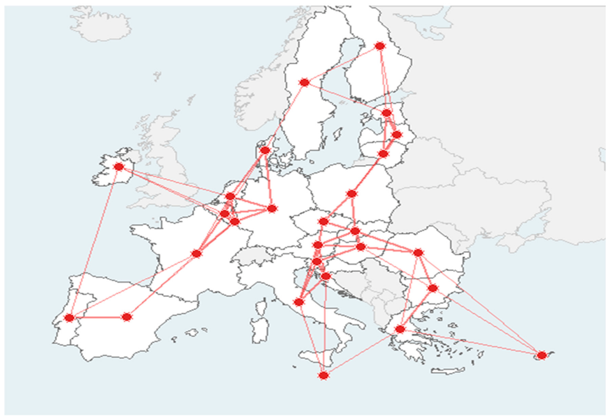
The spatial analysis was conducted after defining a spatial weights matrix $W$ representing the proximity structure among countries. Representative points for each EU country were obtained using the st_point_on_surface function from the R package sf (version 1.0-21). Geographic data were projected to the ETRS89/LAEA Europe coordinate reference system (EPSG:3035), so inter-country distances were calculated as planar projected distances in meters. Spatial connectivity was defined using a three-nearest-neighbor criterion and subsequently symmetrized using the union of directed nearest-neighbor links, such that two countries were considered neighbors whenever either country was among the three nearest neighbors of the other. For each connected pair of countries i and j, the spatial weight $w_{ij}$ was defined as $w_{ij}=1/d_{ij}$, where dij denotes the projected distance between their representative points; for non-neighboring countries, $w_{ij}=0$. This inverse-distance specification assigns greater weight to geographically closer countries and corresponds to a distance-decay exponent of one. Finally, the matrix was row-standardized so that the spatial weights associated with each country summed to one. Although the underlying neighborhood relation was symmetric, row standardization does not necessarily preserve symmetry in the final weights matrix. The resulting specification produced a single connected spatial network comprising all 27 EU Member States, including island countries [47].

The alternative spatial panel specifications can be represented with the following general model:

$${CL}_{it}=\rho {\displaystyle \sum _{j=1}^N}{w}_{ij}{CL}_{it}+ {X^{\prime }}_{it}B+{\mu }_i+{\tau }_t+u_{it}, u_{it}=\lambda {\displaystyle \sum _{j=1}^N}{w}_{ij}{u}_{it}+{\epsilon }_{it}$$

(2)

where $X_{it}$ contains the six WHR explanatory variables defined in Equation (1), $w_{ij}$ is the corresponding element of the spatial weights matrix W, ρ measures spatial dependence in the dependent variable, and λ measures spatial autocorrelation in the disturbance term. The four specifications compared in the empirical analysis can be obtained as particular cases of Equation (2). The non-spatial RE model imposes ρ = 0 and λ = 0, the SAR-RE model allows ρ ≠ 0 while imposing λ = 0, the SEM-RE model imposes ρ = 0 while allowing λ ≠ 0, and the SARAR-RE model allows both spatial parameters to differ from zero.

Once the spatial weights matrix had been defined, the global spatial autocorrelation of happiness was analyzed using Moran’s I. The spatial autocorrelation of the explanatory variables was also examined to assess whether the determinants of happiness themselves exhibited a territorial structure. Next, Moran’s I was calculated for the residuals of the previously selected non-spatial panel model, keeping the same sample, explanatory variables, and structure of individual and time effects. This provided an initial diagnostic of whether spatial dependence remained after accounting for observed determinants, country heterogeneity, and common year effects.

The nature of any remaining spatial dependence was then examined using the standard and locally robust Lagrange multiplier tests for spatial lag and spatial error dependence [48]. The LM-lag and LM-error tests evaluate the presence of each form of spatial dependence separately, whereas their robust counterparts assess one form while allowing for the possible presence of the other [49]. These diagnostics were complemented by the Baltagi–Song–Koh tests, which are specifically designed for panel data and make it possible to distinguish between country random effects and spatial error correlation. In particular, the marginal and conditional tests assess whether random country effects remain necessary when spatial error dependence is allowed for and whether spatial error correlation remains significant once random effects are taken into account [50].

To further assess whether an explicit spatial specification improved the model, four comparable specifications were estimated: the non-spatial random-effects model (RE), the spatial autoregressive random-effects model (SAR-RE), the spatial error random-effects model (SEM-RE), and the spatial autoregressive model with spatially autocorrelated errors (SARAR-RE). These models retained the same explanatory variables and year fixed effects and were compared using the significance of their spatial parameters, log-likelihood values, and Akaike’s information criterion (AIC). Finally, likelihood-ratio tests were used for the nested model comparisons to determine whether the addition of spatial lag or spatial error parameters produced a statistically significant improvement in fit. Since SAR-RE and SEM-RE are not nested, their relative fit was assessed using log-likelihood and AIC rather than a likelihood-ratio test.

Omitting significant spatial dependence may lead to an incomplete specification. In models with a spatial lag, conventional estimators may be biased and inconsistent, whereas when autocorrelation is concentrated in the error term, estimates may lose efficiency and standard errors and significance tests may be incorrect [40]. Accordingly, the final model selection was based on the combined evidence provided by residual Moran’s I, the standard and robust LM tests, the Baltagi–Song–Koh tests, the significance of the spatial parameters, information criteria, likelihood-ratio tests, and coefficient stability. This procedure allowed for an explicit assessment of whether a spatial specification was required or whether the non-spatial random-effects model with year fixed effects adequately captured the structure of the data.

3.2.3. Sensitivity and Robustness Analyses

Several sensitivity analyses were conducted to assess the robustness of the main findings. First, the influence of missing-data treatment was examined by re-estimating the main random-effects model and the spatial autocorrelation tests using only complete observations, thereby excluding the seven country-year observations containing imputed values. Second, potential influential observations were assessed through standardized residuals and a leave-one-country-out procedure, in which the model was re-estimated sequentially after excluding each of the 27 countries. Third, the sensitivity of the spatial results to the definition of the neighborhood structure was examined by reconstructing the spatial weights matrix using four and five nearest neighbors instead of the baseline three-nearest-neighbor specification, while retaining the same inverse-distance weighting, symmetrization procedure, and row standardization.

The statistical and spatial analyses were conducted in R. Data preparation, transformation, and organization were performed mainly using the dplyr, tidyr, and zoo packages, with zoo used for the interpolation of missing values. Non-spatial panel models were estimated with plm, whereas the SAR-RE, SEM-RE, and SARAR-RE models were estimated with splm. Spatial dependence tests were implemented using splm and spdep. Geographic data management, coordinate transformations, and the construction of spatial objects were carried out with sf. European national boundaries were obtained using rnaturalearth, and the maps and other graphical outputs were produced with ggplot2, supported by tibble, purrr, and scales for organizing the results and preparing the figures.

4. Results

4.1. Determination of the Panel Data Model Without Considering Spatial Characteristics

Pairwise correlations and variance inflation factors were examined before estimating the panel models.

Table 2. Pairwise correlations and variance inflation factors of the explanatory variables.

Variable	GDP	SSUP	LEX	FREE	GENR	CORR	VIF
GDP	1						2.635
SSUP	−0.015	1					1.85
LEX	0.567	−0.077	1				1.544
FREE	0.298	0.634	0.178	1			2.412
GENR	0.556	0.261	0.389	0.513	1		1.855
CORR	−0.729	−0.140	−0.494	−0.478	−0.574	1	2.661

Notes: Entries are Pearson correlation coefficients. VIF denotes the variance inflation factor calculated for the six explanatory variables.

shows that the largest absolute correlation was observed between GDP and CORR (r = −0.729), while VIF values ranged from 1.544 to 2.661. These results provide no evidence of problematic multicollinearity among the explanatory variables.

Table 3. Selection of the panel-data specification.

Test	Null Hypothesis	Statistic	df	p-Value	Decision
F test for individual effects	No country-specific effects; pooled OLS is adequate	28.005	26, 237	<0.001	Reject pooled OLS
Breusch–Pagan LM test	No random country effects; pooled OLS is adequate	581.63	1	<0.001	Reject pooled OLS
Hausman test	Random-effects estimator is consistent	3.935	15	0.998	Do not reject random effects
Mundlak CRE joint test (cluster-robust)	Coefficients of country-specific regressor means are jointly zero	2.560	6	0.862	Do not reject random effects
F test for time effects	No common year effects	16.269	9, 228	<0.001	Include year fixed effects
Pesaran CD test	Cross-sectional independence	−1.817	—	0.069	Do not reject cross-sectional independence

Notes: The panel is balanced and contains 27 countries observed over ten years, for a total of 270 observations. The tests support a model with country random effects and year fixed effects. The Pesaran CD test evaluates general cross-sectional dependence.

reports the tests used to determine the appropriate panel-data specification. The F test for individual effects strongly rejects the pooled OLS model, indicating substantial unobserved heterogeneity across countries. The Breusch–Pagan LM test also rejects the absence of country-level random effects, confirming that a pooled specification is inadequate. The Hausman test does not reject the consistency of the random-effects estimator, p = 0.998, suggesting that the unobserved country-specific effects are not systematically correlated with the explanatory variables. To address the possibility that unobserved country-specific heterogeneity may be correlated with the regressors, the Hausman test was complemented with a correlated random-effects specification. Country-specific means of all time-varying regressors were added to the random-effects model and tested jointly. The null hypothesis that all Mundlak terms were jointly equal to zero could not be rejected, either using the conventional covariance matrix (χ²(6) = 3.543; p = 0.738) or using country-clustered robust standard errors (χ²(6) = 2.560; p = 0.862). These results provide additional support for the random-effects specification, although they do not constitute proof of strict exogeneity.

Random effects were therefore preferred to country fixed effects because they are more efficient under this assumption and preserve both within-country and between-country variation. The test for time effects is also significant, p < 0.001, indicating that common shocks and temporal changes affected all EU countries during the study period. Year fixed effects were therefore included.

Finally, the Pesaran CD test does not reject general cross-sectional independence, p = 0.069. However, notice that this result does not preclude geographically structured dependence, since the Pesaran CD test assesses general cross-sectional dependence, whereas Moran’s I evaluates dependence according to the specific spatial structure defined by the weights matrix.

Once the random-effects model with year fixed effects had been selected as the preferred panel-data specification, diagnostic tests were conducted for serial correlation and heteroskedasticity. Serial correlation was strongly detected by both the Wooldridge test (F = 153.790; p < 0.001) and the Breusch–Godfrey/Wooldridge panel test (χ²(10) = 81.778; p < 0.001). Heteroskedasticity was also detected using the studentized Breusch–Pagan test applied to an auxiliary pooled regression containing the same explanatory variables and year effects (BP = 52.641; p < 0.001). Consequently, inference for the final RE model was based on heteroskedasticity- and serial-correlation-robust standard errors clustered at the country level. The estimates are in

Table 4. Non-spatial random-effects panel model with year fixed effects.

Variable	b	β	SE	z-Statistic	p-Value
Intercept	−9.004	---	6.200	−1.452	0.148
GDP	0.653	0.357	0.295	2.211	0.028
SSUP	1.988	0.302	0.668	2.978	0.003
LEX	1.493	0.069	1.415	1.054	0.293
FREE	1.053	0.222	0.267	3.943	<0.001
GENR	0.513	0.107	0.365	1.411	0.159
CORR	−0.822	−0.314	0.219	−3.762	<0.001
Year 2016	0.054	---	0.034	1.586	0.114
Year 2017	0.125	---	0.040	3.125	0.002
Year 2018	0.217	---	0.067	3.230	0.001
Year 2019	0.627	---	0.086	7.268	<0.001
Year 2020	1.004	---	0.170	5.915	<0.001
Year 2021	0.805	---	0.159	5.059	<0.001
Year 2022	0.521	---	0.104	5.021	<0.001
Year 2023	0.478	---	0.089	5.373	<0.001
Year 2024	0.392	---	0.098	3.991	<0.001

Notes: b = coefficient and β = standardized coefficient. SE = standard error. The balanced panel comprises 27 countries, 10 years, and 270 observations. Year 2015 is the reference category. Country-effect variance = 0.0733; idiosyncratic variance = 0.0195; share of variance attributable to country effects = 0.790; idiosyncratic share = 0.210; R² = 0.636; adjusted R² = 0.615; Wald statistic = 443.929; df = 15; model p-value < 0.001. Standardized coefficients are reported only for the continuous explanatory variables. Year fixed effects are binary indicators and are therefore reported in their original metric relative to the reference year (2015).

.

Table 4 shows that GDP has a positive and statistically significant association with happiness, with a coefficient (b) = 0.6527 (p = 0.028), as does SSUP (b = 1.9881; p = 0.003), while CORR is negatively and significantly associated with CL (b = −0.8224; p < 0.001). Freedom also shows a positive and statistically significant association (b = 1.0532; p < 0.001), whereas generosity, although positively associated with happiness (b = 0.5149), does not reach statistical significance (p = 0.159). Healthy life expectancy also does not reach statistical significance (p = 0.293). Taking 2015 as the reference year, no significant difference is observed for 2016, whereas significant positive differences in happiness are found for 2017 (b = 0.1246; p = 0.002), 2018 (b = 0.2165; p = 0.001), 2019 (b = 0.6276; p < 0.001), 2020 (b = 1.0042; p < 0.001), 2021 (b = 0.8048; p < 0.001), 2022 (b = 0.5206; p < 0.001), 2023 (b = 0.4782; p < 0.001), and 2024 (b = 0.3923; p < 0.001). In standardized terms, GDP showed the largest association with happiness (β = 0.357), followed by CORR (β = −0.314), SSUP (β = 0.302), and FREE (β = 0.222). The standardized coefficients of GENR (β = 0.107) and LEX (β = 0.069) were smaller and statistically non-significant.

Table 4 also shows that 79.0% of the residual variance is attributable to persistent differences between countries, compared with 21.0% corresponding to the idiosyncratic component, which reinforces the case for incorporating country effects. Accordingly, the model, based on Equation (1), was estimated using country random effects and year fixed effects.

It is noteworthy that the estimated year effects fluctuate considerably over time. Relative to 2015, they increase from 0.054 in 2016 to 0.125 in 2017, 0.216 in 2018, and 0.628 in 2019, reaching a maximum of 1.004 in 2020. They then decline progressively to 0.805 in 2021, 0.521 in 2022, 0.478 in 2023, and 0.392 in 2024. Consistently, the average temporal effect was 0.205 during the pre-pandemic period (2015–2019), increased markedly to 0.702 during 2020–2023, and fell to 0.392 in 2024. A joint Wald test strongly rejected the hypothesis that the temporal effects were equal across these three periods (Wald χ²(2) = 28.487; p < 0.001). Thus, the results indicate a pronounced temporal shift during 2020–2023, followed by a partial reversal in 2024 toward pre-pandemic levels, although the estimated 2024 effect remained above the 2015–2019 average. These temporal effects should be interpreted as conditional associations rather than causal effects of the COVID-19 pandemic or subsequent economic and geopolitical events.

4.2. Assessment of the Spatial Dependence of Happiness in the EU

4.2.1. Spatial Pattern and Autocorrelation of Happiness

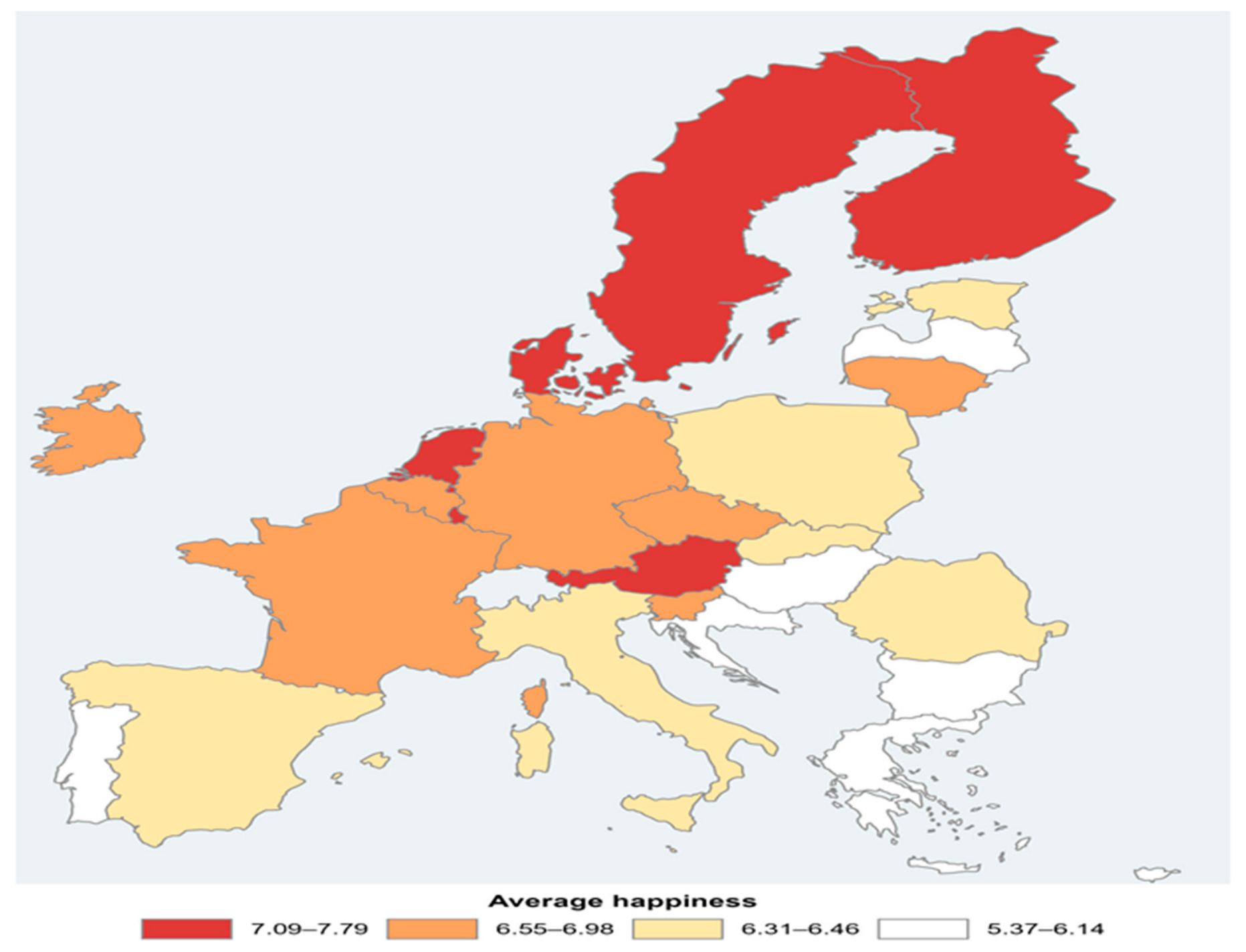
The choropleth map presented in Figure 3 intuitively reveals a clear geographic pattern in the distribution of average happiness across the European Union. The highest values are concentrated mainly in the Nordic countries, as well as in some countries in Central and Northwestern Europe, including the Netherlands, Luxembourg, and Austria. Most of Western and Central Europe shows intermediate levels, while the lowest values are located predominantly in Southern and Eastern Europe, including several countries with a post-communist past. There are, however, some exceptions. For example, Slovenia occupies an intermediate-to-high position among post-communist countries, whereas Croatia remains among the countries with the lowest average happiness. These visual groupings suggest the existence of a spatial structure in happiness levels, which must be formally tested through spatial autocorrelation tests.

Figure 4 graphically represents the connection structure generated by the primary spatial matrix. The network is constructed from a symmetric three-nearest-neighbor relation, so that each country is connected to its three geographically nearest neighbors and also to any additional countries for which it is itself among their three nearest neighbors. The figure therefore shows the spatial structure through which geographic dependence of happiness across countries is represented. It also confirms that all Member States, including island countries, are integrated into a single connected spatial network and illustrates the resulting connectivity among nearby territories.

Table 5. Moran’s I for happiness and residuals of the non-spatial panel model.

Period	Happiness: Moran’s I	p-Value	Monte Carlo p-Value	Residuals: Moran’s I	p-Value	Monte Carlo p-Value
2015	0.428	<0.001	0.002	−0.129	0.758	0.743
2016	0.464	<0.001	0.002	−0.030	0.476	0.455
2017	0.425	<0.001	0.001	0.311	0.004	0.006
2018	0.387	<0.001	0.001	−0.011	0.416	0.409
2019	0.421	<0.001	0.001	0.165	0.048	0.070
2020	0.463	<0.001	0.001	0.211	0.030	0.048
2021	0.437	<0.001	0.001	0.006	0.370	0.337
2022	0.423	<0.001	0.002	0.028	0.307	0.298
2023	0.427	<0.001	0.001	0.068	0.206	0.195
2024	0.423	<0.001	0.005	0.006	0.367	0.337
All years	0.452	<0.001	0.001	0.034	0.2016	0.061

Notes: Residuals correspond to the final non-spatial model with country random effects and year fixed effects. Analytical and Monte Carlo tests use the one-sided alternative of positive spatial autocorrelation. Monte Carlo p-values are based on 999 permutations. For each annual statistic, permutations were performed across countries within the corresponding year. For the pooled statistics, a block-diagonal spatial weights matrix was used and permutations were restricted within each year, so observations were never permuted across different years. Consequently, the pooled test captures contemporaneous spatial dependence while preserving the panel’s temporal structure.

shows a positive, high, and statistically significant spatial autocorrelation of CL in all the years analyzed. Moran’s I values range between 0.387 and 0.464, with Monte Carlo p-values ranging from 0.001 to 0.005, while the pooled value for the whole period is 0.452, with a Monte Carlo p-value of 0.001 based on permutations restricted within each year. These results indicate that geographically close countries tend to show similar happiness levels and that this spatial pattern remains notably stable between 2015 and 2024. This stability is also observed across the pandemic period: average Moran’s I was 0.425 in 2015–2019, 0.438 in 2020–2023, and 0.423 in 2024. Thus, the marked temporal changes detected in the year effects were not accompanied by a comparable alteration in the geographic clustering of happiness.

The non-spatial panel model absorbs a substantial part of this geographic structure. The autocorrelation of its residuals is positive and statistically significant only in 2017, with a Moran’s I of 0.312 and a Monte Carlo p-value of 0.006, and in 2020, with an index of 0.211 and a Monte Carlo p-value of 0.048. In 2019, Moran’s I is 0.165, but the corresponding Monte Carlo p-value is 0.070 and therefore does not reach statistical significance at the 5% level. In the remaining years, the residual indices are relatively small and are not statistically significant. Moreover, when all observations are considered jointly, the residuals do not retain significant spatial dependence, with a Moran’s I of 0.034 and a Monte Carlo p-value of 0.061 based on 999 permutations restricted within each year. Therefore, the random-effects model with year fixed effects explains most of the spatial pattern of happiness and, when the full period is considered, leaves no statistically significant residual spatial dependence.

Table 6. Global Moran’s I for the explanatory variables, 2015–2024.

Variable	Moran’s I	p-Value
GDP	0.524	<0.001
SSUP	0.832	<0.001
LEX	0.42	<0.001
FREE	0.467	<0.001
GENR	0.255	<0.001
CORR	0.58	<0.001

shows that the strong spatial clustering observed for happiness is also present in all its explanatory factors. Global Moran’s I values are positive and statistically significant for GDP (I = 0.524), social support (I = 0.832), healthy life expectancy (I = 0.420), freedom (I = 0.467), generosity (I = 0.255), and perceptions of corruption (I = 0.580), with p < 0.001 in all cases. This finding indicates that the socioeconomic, social, health-related and institutional determinants of happiness are themselves strongly geographically clustered across EU countries. Accordingly, the marked spatial autocorrelation observed in happiness levels may largely reflect the spatial concentration of these underlying determinants. This interpretation is consistent with the sharp reduction in spatial autocorrelation once these factors, country heterogeneity, and year effects are controlled for.

4.2.2. Spatial Dependence Diagnostics

Table 7. Anselin LM and robust LM tests.

Test	Statistic	p-Value	Conclusion
LM spatial lag	1.826	0.177	No spatial lag dependence
LM spatial error	1.445	0.229	No spatial error dependence
Robust LM spatial lag	0.397	0.529	No spatial lag dependence
Robust LM spatial error	0.016	0.901	No spatial error dependence

reports the standard and locally robust Lagrange Multiplier tests for spatial dependence [49]. Neither the LM test for a spatial lag (LM = 1.826; p = 0.177) nor the LM test for spatial error dependence (LM = 1.445; p = 0.229) is statistically significant. The locally robust versions lead to the same conclusion: the robust LM-lag test yields a statistic of 0.397 (p = 0.529), while the robust LM-error test produces a statistic of 0.016 (p = 0.901). Therefore, once country heterogeneity and common year effects are controlled for, the results provide no evidence of either a spatial lag process or residual spatial error dependence. The agreement between the standard and robust tests reinforces the conclusion that an additional spatial component is not required by the data.

Table 8. Baltagi–Song–Koh tests for random effects and spatial error correlation.

Test	Component Evaluated	Statistic	p-Value	Result
SLM1	Random country effects, assuming no spatial error correlation	30.552	<0.001	Random effects are present
SLM2	Spatial error correlation, assuming no random effects	−1.041	0.298	Not significant
LM-H	Joint presence of random effects and/or spatial error correlation	757.640	<0.001	Joint null rejected
CLM-λ	Spatial error correlation, allowing for random effects	1.029	0.304	Spatial error correlation is not significant
CLM-μ	Random effects, allowing for spatial error correlation	24.941	<0.001	Random effects remain necessary

presents the tests by Baltagi–Song–Koh [50]. The SLM1 test rejects the absence of random effects (statistic = 30.552; p < 0.001), while SLM2 does not detect spatial autocorrelation of the error when it is assumed that no random effects exist (statistic = −1.041; p = 0.298). This latter result, however, should be interpreted with caution, since it starts from a hypothesis that is incompatible with the clear presence of national heterogeneity. The joint LM-H test clearly rejects the simultaneous absence of both components (statistic = 757.640; p < 0.001). More importantly, the conditional tests show that spatial autocorrelation of the error is not significant once random effects are admitted (CLM-λ = 1.029; p = 0.304), whereas random effects continue to be necessary when spatial dependence is allowed for (CLM-μ = 24.941; p < 0.001). Taken together, these results support the presence of substantial unobserved heterogeneity between countries but do not provide evidence of an additional spatial error component, reinforcing the selection of the non-spatial random-effects model with year fixed effects as the preferred specification.

Table 9. Comparison of spatial panel specifications.

Model	φ	p-Value	ρ	p-Value	λ	p-Value	LogLik	AIC
RE	4.2074	<0.001	—	—	—	—	102.5550	−169.1100
SAR-RE	4.2685	<0.001	0.0708	0.2827	—	—	103.1289	−168.2578
SEM-RE	4.2387	<0.001	—	—	0.0936	0.2839	103.1173	−168.2346
SARAR-RE	4.2501	<0.001	0.0419	0.6750	0.0521	0.6995	103.2035	−166.4070

Note: All models include country random effects and year fixed effects and are estimated using the same balanced panel of 27 countries and 270 observations. φ denotes the variance ratio associated with the country-specific random effect; ρ is the spatial autoregressive coefficient of the dependent variable, and λ is the spatial autocorrelation coefficient of the error term. RE refers to the non-spatial random-effects model, SAR-RE incorporates a spatial lag of the dependent variable, SEM-RE incorporates spatial dependence in the error term, and SARAR-RE includes both components. LogLik denotes the log-likelihood, whereas AIC is Akaike’s information criterion, with lower values indicating a better relative model fit. Dashes indicate parameters that are not included in the corresponding model specification.

and

Table 10. Likelihood-ratio tests between nested models.

Comparison	LR Statistic	p-Value	Conclusion
SAR-RE versus RE	1.148	0.284	SAR does not improve the non-spatial model.
SEM-RE versus RE	1.125	0.289	SEM does not improve the non-spatial model.
SARAR-RE versus SAR-RE	0.149	0.699	Adding spatial error correlation is not justified.
SARAR-RE versus SEM-RE	0.172	0.678	Adding a spatial lag is not justified.

Notes: SAR and SEM are not nested and therefore cannot be compared directly using a likelihood-ratio test. Because both contain the same number of parameters, their log-likelihoods and information criteria are directly comparable.

make it possible to assess, through model comparisons, the gain obtained by incorporating spatial dependence into the random-effects specification. The alternative models reported in Table 9 correspond to the restrictions on ρ and λ described in Equation (2). It shows that both the spatial autoregressive random-effects model (SAR-RE) and the spatial error random-effects model (SEM-RE) present slightly higher log-likelihood values than the non-spatial RE model. However, neither the spatial autoregressive parameter in the SAR-RE model nor the spatial error parameter in the SEM-RE model is statistically significant. Moreover, both models present slightly higher Akaike’s information criterion (AIC) values than the non-spatial RE model. In the spatial autoregressive model with spatially autocorrelated errors (SARAR-RE), neither of the two spatial parameters is significant, and its greater complexity does not translate into an improvement in AIC. The likelihood-ratio tests in Table 10 confirm that neither SAR-RE nor SEM-RE significantly improves on the RE model, while SARAR-RE improves on neither SAR-RE nor SEM-RE. Since SAR-RE and SEM-RE are not nested models, they cannot be compared directly using this test; however, since they contain the same number of parameters, they can be compared on the basis of log-likelihood and AIC. In this respect, SAR-RE and SEM-RE offer virtually identical fits, but neither improves on the more parsimonious non-spatial RE specification. Overall, the combined evidence supports the selection of the non-spatial RE model with year fixed effects as the preferred specification.

4.3. Sensitivity and Robustness Analyses

The complete-case analysis (N = 263) produced results closely aligned with those of the imputed sample. All coefficient signs were preserved, and the inferential conclusions remained unchanged under country-clustered robust standard errors: GDP, SSUP, FREE, and CORR remained statistically significant, whereas LEX and GENR remained non-significant. Happiness also remained significantly spatially autocorrelated in every year, while residual spatial dependence remained generally absent.

The influence diagnostics likewise indicated substantial stability. Only three observations had absolute standardized residuals above 3, representing 1.1% of the sample. In the leave-one-country-out analysis, all coefficients retained their signs across the 27 re-estimations. FREE and CORR remained significant in all cases, and GDP and SSUP remained significant in 26 of the 27 specifications, whereas LEX and GENR remained non-significant in 26 of 27 specifications.

Finally, the spatial results were robust to alternative neighborhood definitions. Using four and five nearest neighbors, pooled Moran’s I for happiness remained positive and highly significant (I = 0.420 and I = 0.430, respectively; Monte Carlo p = 0.001 in both cases), whereas residual spatial autocorrelation remained non-significant (I = 0.011, p = 0.106; and I = −0.004, p = 0.163). The alternative SAR-RE, SEM-RE, and SARAR-RE specifications did not significantly improve the non-spatial RE model, which retained the lowest AIC under both alternative matrices.

5. Discussion

5.1. General Discussion

Regarding the first research objective (RO1), in terms of the hypotheses formulated in this study, H1a, H1b, H1d, and H1f are supported but H1c and H1e are not. The panel data model reveals SSUP and GDP as key explanatory factors associated with happiness. Likewise, the use of year fixed effects together with country random effects proves to be the most appropriate panel data specification. This result is consistent with mainstream WHR findings, which identify both factors as major determinants of happiness [22,51,52,53].

The relevance attained by CORR is particularly striking. In analyses covering a broad and heterogeneous set of countries, this variable typically shows lower explanatory power than GDP per capita or social support, and even lower than other factors such as healthy life expectancy or freedom to make life choices [8]. In the present study, by contrast, its association is statistically significant and shows robustness comparable to those of GDP and SSUP. This result suggests that the relative importance of the determinants of happiness depends on the geographic and institutional context under analysis, as has been shown in various settings [54]. A possible explanation for the pronounced association between perceptions of corruption and happiness lies in its effects on trust and perceived justice. Corruption can reduce wellbeing even when citizens do not experience it directly, since it erodes trust in government and institutions, generates a sense of inequality and injustice, and fosters negative emotions, insecurity, and hopelessness, effects that may be more pronounced in democratic countries [55].

Recent studies show that both happiness levels and the strength of their associations with various economic and social factors vary significantly across European and global regions [54]. A similar pattern has also been observed within Europe. In Western and Northern European countries, perceptions of corruption show a strong and significant association with happiness, while healthy life expectancy fails to reach statistical significance in any of the years analyzed [14]. This result is consistent with evidence that the relationship between healthy life expectancy and happiness tends to weaken in high-income economies, while the adverse effects of corruption are more visible in wealthy, democratic, and Western countries [30].

With respect to RO2, H2a is supported, as happiness exhibits strong and persistent positive spatial autocorrelation throughout the 2015–2024 period. However, H2b is not supported: once the standard WHR determinants, country random effects, and year fixed effects are incorporated, no robust residual spatial dependence remains. The results show that incorporating the spatial dimension provides substantive information about the territorial organization of happiness, even though it does not ultimately require a spatial econometric specification. Happiness levels display a positive, high, and stable spatial autocorrelation throughout the period, indicating that nearby countries tend to report similar life evaluations. However, the basic WHR model with country random effects and year fixed effects absorbs most of this spatial pattern, and no statistically significant residual spatial dependence remains when the full period is considered. This result is reinforced by the spatial diagnostic tests and model comparisons, which provide no evidence that either a spatial lag or a spatial error component significantly improves the non-spatial random-effects specification.

An important element for interpreting this result is that the six explanatory factors are themselves geographically clustered. Global Moran’s I is positive and statistically significant for GDP per capita, social support, healthy life expectancy, freedom, generosity, and perceptions of corruption. Thus, the spatial concentration of happiness across EU countries appears to be closely associated with the spatial concentration of its underlying socioeconomic, social, health, and institutional determinants. Geographic proximity is therefore descriptively informative, but much of this information is already captured by variables that are themselves territorially structured.

From a conceptual standpoint, this result implies that countries should not be understood as isolated units. Location places them within regional environments in which institutional, cultural, historical, environmental, and economic conditions are shared. The spatial literature has indeed pointed out that place and the characteristics of neighboring territories can shape wellbeing, and that ignoring this dimension can lead to an incomplete representation of its determinants [9,11]. In this sense, space does not necessarily act as an additional explanatory mechanism, but rather as the structure through which multiple conditions relevant to happiness are geographically organized.

The absence of significant residual spatial dependence also helps clarify the nature of this relationship. The similarity between nearby countries does not appear to reflect a systematic direct transmission of happiness between neighboring Member States, nor an additional spatially correlated error process once the standard WHR determinants, persistent country heterogeneity, and common temporal effects are taken into account. Instead, the evidence suggests that geographically close countries tend to resemble one another because many of the factors associated with happiness are themselves spatially clustered. This distinction is important because observed spatial clustering should not automatically be interpreted as evidence of spatial spillovers or “contagion”.

This interpretation also provides a rationale for research that extends the basic WHR model. The incorporation of new variables should not be conceived solely as a strategy for improving statistical fit, but as an attempt to identify the broader territorial mechanisms underlying the spatial concentration of both happiness and its determinants. Institutional, cultural, environmental, and regional characteristics may help explain why neighboring countries display similar levels of GDP, social support, health, freedom, generosity, corruption perceptions, and ultimately happiness. Future research could therefore examine more explicitly the processes through which these characteristics become geographically clustered and whether specific regional contexts generate additional spatial effects under particular circumstances.

The findings are consistent with previous spatial econometric studies of happiness, though they introduce an important nuance. Aral and Bakır [9] observe clusters of countries with similar happiness levels and conclude that ignoring the spatial dimension may yield an incomplete explanation of the relationship between wellbeing and economic conditions. Stanca [11] likewise argues that geography, culture, and institutions should be explicitly incorporated when analyzing international differences in wellbeing. Lin et al. [32] find spatial dependence and indirect effects between countries, attributed to both the happiness and the socioeconomic conditions of neighboring territories. Ziogas [12] documents clustering and spillovers of life satisfaction between communities and notes that shared cultural and institutional traits may explain part of these interdependencies.

The main contribution of the spatial analysis is therefore not to confirm the familiar north–south or west–east pattern of European wellbeing. Rather, it is to show that this descriptive geography substantially weakens once the standard WHR determinants, country-specific heterogeneity, and common year effects are taken into account. Moreover, all six explanatory factors are themselves spatially autocorrelated. This indicates that the observed clustering of happiness is largely associated with the territorial concentration of its underlying determinants, rather than with an autonomous spatial spillover process.

5.2. Theoretical and Practical Implications

From a theoretical perspective, the results show that the use of panel data and the correct choice between fixed and random effects are essential for controlling national heterogeneity and temporal evolution, but they should also be complemented by an explicit examination of the spatial structure of happiness. Conventional panel models maintain the assumption that, once explanatory variables and individual and time effects are accounted for, countries are spatially independent. In the present study, happiness displays strong spatial autocorrelation, but this dependence largely disappears in the residuals of the non-spatial model, and neither the SAR-RE nor the SEM-RE specification significantly improves on the random-effects model with year fixed effects. Moreover, all six WHR determinants are themselves significantly spatially autocorrelated. These results suggest that the geographic clustering of happiness largely reflects the spatial concentration of its underlying socioeconomic, social, health, and institutional determinants rather than an additional independent spatial process. This result aligns with [9], who warn that ignoring heterogeneity and spatial dependence can obscure relevant differences and affect the validity of inference, and with [10], who show that incorporating territorial factors can improve understanding of the determinants of wellbeing.

The absence of significant residual spatial dependence further provides a specific theoretical interpretation. The spatial structure detected does not appear to stem primarily from a direct transmission of happiness between countries or from omitted factors generating an additional spatially correlated error process. Instead, the basic WHR determinants themselves exhibit a marked territorial structure. The basic WHR model therefore provides a relevant explanation of the geographic distribution of wellbeing, although it does not necessarily exhaust the territorial, institutional, cultural, environmental, and economic conditions that shape it. This evidence supports lines of research that extend the WHR model through new variables (e.g., [14,15,16,17,18,20,55]), but it also indicates that such extensions should explicitly consider how these factors are distributed in space. The same recommendation applies to other frameworks used to explain happiness, such as those based on the Sustainable Development Goals [56,57,58]. Examining the presence of spatial dependence, and incorporating it through appropriate models where it persists after controlling for observed determinants and country and time effects, seems a promising line of inquiry, since levels of SDG compliance and their relationships with happiness may also be territorially clustered.

From a practical standpoint, social support maintains a positive, strong, and robust association across the main specifications. This result indicates that wellbeing-oriented policies must not take into account economic growth alone, but should also seek to strengthen social cohesion, interpersonal trust, family and community networks, and people’s ability to obtain help when needed. However, since the variables are measured on different scales, the magnitude of the coefficients does not allow us to directly claim that social support is the “most important” factor. It can instead be regarded as one of the strongest and most consistent determinants in the model.

The relevance attained by perceptions of corruption also carries notable implications for the EU. The results suggest that transparency, accountability, and integrity in public and private management not only have value from a normative standpoint, but also are associated with how citizens evaluate their lives. In this sense, strengthening institutional controls, ethical codes, the independence of oversight bodies, and mechanisms for preventing and sanctioning corruption may contribute to wellbeing. Better governance may also indirectly foster other determinants of happiness by increasing institutional trust, improving the provision of public services, and facilitating the achievement of economic, social, and environmental goals.

Finally, the spatial evidence suggests caution when drawing policy implications from geographic clustering. The results do not support a direct transmission of happiness between neighboring countries, nor do they indicate that regional coordination itself necessarily increases wellbeing. Rather, they show that nearby EU countries tend to share similar socioeconomic, social, health, and institutional conditions, many of which are themselves spatially clustered. From a policy perspective, this suggests that European coordination may be useful when addressing common regional conditions—such as social cohesion, institutional quality, and regional development—but such coordination should not be interpreted as a mechanism through which happiness automatically spills over across borders.

6. Conclusions

6.1. Main Findings

Happiness in the EU displays a clear and persistent territorial structure. Nearby countries show similar wellbeing levels, and this spatial concentration remains stable throughout the 2015–2024 period. However, the panel model with country random effects and year fixed effects explains most of this pattern, and no significant residual spatial dependence remains when the full period is considered. Moreover, the six WHR determinants are themselves significantly spatially autocorrelated, suggesting that the geographic concentration of happiness largely reflects the spatial distribution of its underlying determinants. Accounting for space is therefore not merely an econometric consideration, but an important element for understanding how happiness is distributed across Member States.

The most robust determinants of the WHR model are GDP per capita, social support, freedom to make life choices, and perceptions of corruption. GDP, social support, and freedom show positive and statistically significant associations with happiness, while higher perceptions of corruption are clearly associated with lower happiness levels. Healthy life expectancy and generosity do not reach statistical significance in the selected specification. These results show that, within a relatively developed and institutionally integrated bloc such as the EU, institutional quality remains a robust correlate of happiness alongside traditional economic and social factors.

The evidence favors the non-spatial random-effects model with year fixed effects. This indicates that the similarity between neighboring countries does not appear to stem primarily from a direct contagion of happiness or from an additional spatially correlated error process, but rather from the fact that the main determinants of happiness are themselves geographically clustered. In practical terms, the results highlight the relevance of economic conditions, social networks, freedom of choice, and institutional integrity for European wellbeing policies. The spatial evidence further suggests that policymakers should take into account the shared socioeconomic and institutional conditions that characterize neighboring countries, without implying that supranational coordination itself necessarily generates higher wellbeing.

6.2. Limitations and Future Research

This study has limitations that should be taken into account when interpreting its results. First, although the panel has been extended to ten years, from 2015 to 2024, the period remains relatively limited for identifying long-term dynamics, structural changes, or lagged adjustments between the World Happiness Report determinants and happiness. It also includes years marked by the COVID-19 pandemic and by subsequent economic and geopolitical disturbances, which may have temporarily altered life evaluations.

The analysis uses national averages. This aggregation allows for comparison across the 27 Member States, but it conceals internal inequalities and differences between regions, cities, and social groups. It also precludes precise identification of the individual-level mechanisms that connect social support, perceptions of corruption, freedom, or other determinants with life satisfaction. The Cantril Ladder, although widely used, is a global measure based on a single question and does not capture all the cognitive and affective dimensions of wellbeing.

The results are associative and do not allow for the establishment of causality. Although happiness and all six WHR determinants display significant spatial clustering, the analysis does not identify the mechanisms responsible for their geographic concentration. Some of the explanatory variables, particularly GDP per capita, social support, and perceptions of corruption, may be jointly determined with happiness, so reverse causality cannot be excluded. The estimated coefficients should therefore be interpreted as conditional associations rather than causal effects. Likewise, the spatial matrix is based on three nearest neighbors and inverse distances; although the results proved robust to specifications using a larger number of nearest neighbors (k = 4 and k = 5), other definitions of proximity could produce different results. Finally, some missing observations in the original data series were obtained through temporal interpolation, which should also be taken into account when interpreting the estimates.

Future research should extend the study period further, use regional data and microdata, and compare different spatial weight matrices. It would also be useful to incorporate institutional, cultural, environmental, historical, and welfare-regime variables to examine more directly the sources of the observed geographic clustering. Other extensions could employ dynamic spatial models, the Durbin model, or multilevel specifications; explore nonlinear relationships and interactions; and examine whether the links between happiness and alternative frameworks, such as the Sustainable Development Goals, display a similar geographic structure.

References

1. Turner, B.S. (I Can’t Get No) Satisfaction: Happiness and successful societies. J. Sociol. 2018, 54, 279–293. [Google Scholar] [CrossRef] [Scilit]
2. Easterlin, R.A. Does economic growth improve the human lot? Some empirical evidence. In Nations and Households in Economic Growth: Essays in Honour of Moses Abramovitz; David, P.A., Reder, M.W., Eds.; Academic Press: New York, NY, USA, 1974; pp. 89–125. [Google Scholar] [CrossRef] [Scilit]
3. Wilson, E.; Mukhopadhyaya, P. The All-You-Can-Eat Economy: How never-ending economic growth affects our happiness and our chances for a sustainable future. World 2020, 1, 216–226. [Google Scholar] [CrossRef] [Scilit]
4. Agrawal, S.; Sharma, N.; Bruni, M.E.; Iazzolino, G. Happiness economics: Discovering future research trends through a systematic literature review. J. Clean. Prod. 2023, 416, 137860. [Google Scholar] [CrossRef] [Scilit]
5. Veenhoven, R. How to take stock of research findings on happiness in regions using the World Database of Happiness. Appl. Res. Qual. Life 2026, 21, 9–33. [Google Scholar] [CrossRef] [Scilit]
6. Helliwell, J.F.; Layard, R.; Sachs, J.D.; De Neve, J.-E.; Aknin, L.B.; Wang, S. (Eds.) World Happiness Report 2025; Wellbeing Research Centre, University of Oxford: Oxford, UK, 2025. [Google Scholar]
7. To, W.-M. A bibliometric analysis of World issues—Social, political, economic, and environmental dimensions. World 2022, 3, 619–638. [Google Scholar] [CrossRef] [Scilit]
8. Torres-Coronas, T.; de Andrés-Sánchez, J. Explaining global happiness: Evidence from decision trees and necessary condition analysis. Economies 2026, 14, 172. [Google Scholar] [CrossRef] [Scilit]
9. Aral, N.; Bakır, H. A spatial analysis of happiness. Panoeconomicus 2024, 71, 135–151. [Google Scholar] [CrossRef] [Scilit]
10. Brereton, F.; Clinch, J.P.; Ferreira, S. Happiness, geography and the environment. Ecol. Econ. 2008, 65, 386–396. [Google Scholar] [CrossRef] [Scilit]
11. Stanca, L. The geography of economics and happiness: Spatial patterns in the effects of economic conditions on well-being. Soc. Indic. Res. 2010, 99, 115–133. [Google Scholar] [CrossRef] [Scilit]
12. Ziogas, T.; Ballas, D.; Koster, S.; Edzes, A. Happiness, space and place: Community area clustering and spillovers of life satisfaction in Canada. Appl. Res. Qual. Life 2023, 18, 2661–2704. [Google Scholar] [CrossRef] [Scilit]
13. Zeitlin, J.; Rangoni, B. How the European Union reconciles uniform regulation with legitimate diversity: Towards a tighter experimentalist governance architecture. J. Eur. Public Policy 2026, 33, 1865–1893. [Google Scholar] [CrossRef] [Scilit]
14. Ionescu-Feleagă, L.; Ionescu, B.-Ş.; Stoica, O.C. The impact of digitalization on happiness: A European perspective. Mathematics 2022, 10, 2766. [Google Scholar] [CrossRef] [Scilit]
15. Detrinidad, E.; López-Ruiz, V.-R. The interplay of happiness and sustainability: A multidimensional scaling and K-means cluster approach. Sustainability 2024, 16, 10068. [Google Scholar] [CrossRef] [Scilit]
16. Mahalik, J.R.; Harris, M.P. Precarious manhood, precarious nations: The contribution of cultural beliefs comprising masculinity to national happiness. Soc. Sci. Med. 2026, 388, 118752. [Google Scholar] [CrossRef] [Scilit] [PubMed]
17. Zong, Y. The research on the factors affecting the World Happiness Index. In Proceedings of the 2nd International Conference on Mathematical Physics and Computational Simulation; EWA Publishing: Oxford, UK, 2024; pp. 104–111. [Google Scholar] [CrossRef] [Scilit]
18. Li, T.; Zhong, J.; Xu, M. Does the credit cycle have an impact on happiness? Int. J. Environ. Res. Public Health 2020, 17, 183. [Google Scholar] [CrossRef] [Scilit]
19. Lago, I.; de Gispert, C.; Bosch, N.; Vilalta, M. Decentralizing happiness. Publius 2025. Available online: https://portalrecerca.csuc.cat/article/doi/10.1093/publius/pjaf012 (accessed on 20 July 2026).
20. Chen, X.; Li, S.; Sowah, J.S.; Zou, S. Soft institutions, hard cash: Societal happiness and corporate cash holdings. Int. Rev. Econ. Financ. 2025, 103, 104506. [Google Scholar] [CrossRef] [Scilit]
21. Pološki Vokić, N.; Klindžić, M. The association between national human resource management practices and measures and correlates of national happiness. Društ. Istraž. 2024, 33, 291–313. [Google Scholar] [CrossRef] [Scilit]
22. Tofallis, C. Which formula for national happiness? Socioecon. Plan. Sci. 2020, 70, 100688. [Google Scholar] [CrossRef] [Scilit]
23. Pereira, M.C.; Coelho, F.; Silva, G.M. Is there a happy culture? Multiple paths to national subjective well-being. Kyklos 2023, 76, 613–641. [Google Scholar] [CrossRef] [Scilit]
24. Trinh, T.A.; Nhieu, N.-L. A r,s,t-spherical fuzzy decision-making model of university happiness: Case study of University of Economics Ho Chi Minh City. Humanit. Soc. Sci. Commun. 2026; in press. [CrossRef] [Scilit]
25. Akanbi, K.; Yeboah, J.; Oluwadare, S.; Nti, I.K. Predicting happiness index using machine learning. In Proceedings of the 2024 IEEE 3rd International Conference on Computing and Machine Intelligence (ICMI), Mt. Pleasant, MI, USA, 13–14 April 2024; IEEE: Piscataway, NJ, USA, 2024; pp. 361–365. [Google Scholar] [CrossRef] [Scilit]
26. Chaouch, M.; Katsaiti, M.-S. On happiness and sustainability comovement: Evidence from regularized regression and semiparametric copula models. Soc. Indic. Res. 2026, 181, 36. [Google Scholar] [CrossRef] [Scilit]
27. Timmapuram, M.; Ramdas, R.; Vutkur, S.R.; Mali, Y.; Vasanth, K. Understanding the regional differences in World Happiness Index using machine learning. In Proceedings of the 2023 International Conference on Innovative Computing, Intelligent Communication and Smart Electrical Systems (ICSES), Chennai, India, 14–15 December 2023; IEEE: Piscataway, NJ, USA, 2023. [Google Scholar] [CrossRef] [Scilit]
28. Çelik, S.; Doğan, İ.; Uçal, M.; Akbulut Küçük, S. Accuracy comparison of machine learning algorithms on World Happiness Index data. Mathematics 2025, 13, 1176. [Google Scholar] [CrossRef] [Scilit]
29. Yang, B.; Xie, X. Analyzing and predicting global happiness index via integrated multilayer clustering and machine learning models. PLoS ONE 2025, 20, e0322287. [Google Scholar] [CrossRef] [Scilit] [PubMed]
30. Kamińska, J.A.; Dionísio, A.; Infante, P.; Carrilho, R. More is still not enough—What is necessary and sufficient for happiness? Sustainability 2025, 17, 6121. [Google Scholar] [CrossRef] [Scilit]
31. Khder, M.A.; Sayfi, M.A.; Fujo, S.W. Analysis of World Happiness Report dataset using machine learning approaches. Int. J. Adv. Soft Comput. Appl. 2022, 14, 15–34. [Google Scholar] [CrossRef] [Scilit]
32. Lin, C.-H.A.; Lahiri, S.; Hsu, C.-P. Happiness and globalization: A spatial econometric approach. J. Happiness Stud. 2017, 18, 1841–1857. [Google Scholar] [CrossRef] [Scilit]
33. Dong, G.; Nakaya, T.; Brunsdon, C. Geographically weighted regression models for ordinal categorical response variables: An application to geo-referenced life satisfaction data. Comput. Environ. Urban Syst. 2018, 70, 35–42. [Google Scholar] [CrossRef] [Scilit]
34. Sarrias, M. Do monetary subjective well-being evaluations vary across space? Comparing continuous and discrete spatial heterogeneity. Spat. Econ. Anal. 2019, 14, 53–87. [Google Scholar] [CrossRef] [Scilit]
35. Velázquez, G.; Linares, S. Análisis de autocorrelación espacial en variables de bienestar en la Argentina. Vegueta 2008, 10, 131–144. [Google Scholar]
36. Vaz, E. A spatial analysis of the Instagram hashtag #happy: An assessment of Toronto. In Geography of Happiness: A Spatial Analysis of Subjective Well-Being; Vaz, E., Ed.; Springer International Publishing: Cham, Switzerland, 2023; pp. 11–32. [Google Scholar] [CrossRef] [Scilit]
37. Pawliczek, A.; Kurowska-Pysz, J.; Smilnak, R. Relation between globe latitude and the quality of life: Insights for public policy management. Sustainability 2022, 14, 1461. [Google Scholar] [CrossRef] [Scilit]
38. Indelicato, A.; Martín, J.C.; Marinello, V. Regional disparities in subjective wellbeing across Europe: A fuzzy hybrid TOPSIS approach. PLoS ONE 2026, 21, e0341119. [Google Scholar] [CrossRef] [Scilit] [PubMed]
39. Lee, Y.A.; Lun, P.; Tay, L.; Cheung, F. Reevaluating the role of geographical regional factors in subjective well-being. Sci. Rep. 2026, 16, 22925. [Google Scholar] [CrossRef] [Scilit] [PubMed]
40. Anselin, L. Spatial Econometrics: Methods and Models; Kluwer Academic Publishers: Dordrecht, The Netherlands, 1988. [Google Scholar] [CrossRef] [Scilit]
41. Hofstede, G. Culture and organizations. Int. Stud. Manag. Organ. 1980, 10, 15–41. [Google Scholar] [CrossRef] [Scilit]
42. Inglehart, R.; Baker, W.E. Modernization, cultural change, and the persistence of traditional values. Am. Sociol. Rev. 2000, 65, 19–51. [Google Scholar] [CrossRef] [Scilit]
43. Ye, D.; Ng, Y.-K.; Lian, Y. Culture and happiness. Soc. Indic. Res. 2015, 123, 519–547. [Google Scholar] [CrossRef] [Scilit] [PubMed]
44. Esping-Andersen, G. The Three Worlds of Welfare Capitalism; Princeton University Press: Princeton, NJ, USA, 1990. [Google Scholar]
45. Ferrera, M. The Southern Model of Welfare in Social Europe. J. Eur. Soc. Policy 1996, 6, 17–37. [Google Scholar] [CrossRef] [Scilit]
46. Baltagi, B.H. Econometric Analysis of Panel Data, 6th ed.; Springer: Cham, Switzerland, 2021. [Google Scholar] [CrossRef] [Scilit]
47. LeSage, J.; Pace, R.K. Introduction to Spatial Econometrics; CRC Press: Boca Raton, FL, USA, 2009. [Google Scholar] [CrossRef] [Scilit]
48. Elhorst, J.P. Spatial Econometrics: From Cross-Sectional Data to Spatial Panels; Springer: Heidelberg, Germany, 2014. [Google Scholar] [CrossRef] [Scilit]
49. Anselin, L.; Bera, A.K.; Florax, R.; Yoon, M.J. Simple diagnostic tests for spatial dependence. Reg. Sci. Urban Econ. 1996, 26, 77–104. [Google Scholar] [CrossRef] [Scilit]
50. Baltagi, B.H.; Song, S.H.; Koh, W. Testing panel data regression models with spatial error correlation. J. Econom. 2003, 117, 123–150. [Google Scholar] [CrossRef] [Scilit]
51. Helliwell, J.F.; Huang, H.; Wang, S. Social capital and well-being in times of crisis. J. Happiness Stud. 2014, 15, 145–162. [Google Scholar] [CrossRef] [Scilit]
52. Chaudhary, M.; Dixit, S.; Sahni, N. Network learning approaches to study world happiness. arXiv 2020, arXiv:2007.09181. [Google Scholar]
53. Zhang, Y. Analyze and predict the 2022 World Happiness Report based on the past year’s dataset. J. Comput. Sci. 2023, 19, 483–492. [Google Scholar] [CrossRef] [Scilit]
54. Çelik, S.; Gökdemir, T.; Çondur, F. Statistical analysis of the World Happiness Index by regions. Qual. Quant. 2025, 59, 4003–4018. [Google Scholar] [CrossRef] [Scilit]
55. Machani, M.; Shtudiner, Z. The effect of corruption priming on happiness and negative emotions. Manag. Decis. Econ. 2026, 47, 457–467. [Google Scholar] [CrossRef] [Scilit]
56. De Neve, J.-E.; Sachs, J.D. The SDGs and human well-being: A global analysis of synergies, trade-offs, and regional differences. Sci. Rep. 2020, 10, 15113. [Google Scholar] [CrossRef] [Scilit] [PubMed]
57. Arana-Barbier, P.J. Does the 2030 agenda generate happiness? A longitudinal approach to the SDGs vs. the well-being of the world. Humanit. Soc. Sci. Lett. 2024, 12, 723–736. [Google Scholar] [CrossRef] [Scilit]
58. Bernardo, S.; Vasconcelos, M.L.; Rocha, F. SDG progress and well-being across the EU: Are we happier yet? Humanit. Soc. Sci. Commun. 2025, 12, 1796. [Google Scholar] [CrossRef] [Scilit]
Figure 1. Framework in this paper.
World 07 00152 g001
Figure 2. Evolution of mean happiness in EU countries, 2015–2024.
World 07 00152 g002
Figure 3. Choropleth map of the distribution of happiness in the EU, 2015–2024. Darker shades indicate higher average happiness levels.
World 07 00152 g003
Figure 4. Spatial network based on the symmetric three-nearest-neighbor matrix used in the analysis. Lines represent the spatial links between EU countries. The red circle indicates the location of each country’s capital.
World 07 00152 g004