Nonlinear Probabilistic Model Predictive Control Design for Obstacle Avoiding Uncrewed Surface Vehicles

Abstract

The primary objective of this research is to develop a probabilistic nonlinear model predictive control structure (NMPC) that efficiently operates uncrewed surface vehicles (USVs) in an environment that has probabilistic disturbances, such as wind, waves, and currents of the water, while simultaneously maneuvering the vehicle in a way that avoids stationary or moving stochastic obstacles in its path. The proposed controller structure considers the mean and covariances of the inputs or state variables of the vehicle in the cost function to handle probabilistic disturbances, where an extended Kalman filter (EKF) is utilized to calculate the mean, and the covariances are calculated dynamically via a linear matrix equality based on this mean and obtained system matrices with successive linearization for every sampling instance. The proposed control structure deals with non-zero-mean probabilistic disturbances such as water current via an innovative approach that treats the mean of the disturbance as a deterministic part, which is estimated by a disturbance observer and eliminated by a control term in the controller in addition to the control signal obtained via MPC optimization; the effect of the remaining zero-mean part is handled over its covariance during the probabilistic MPC optimization. The probabilistic constraints are also dealt with by converting them to deterministic constraints, as in linear probabilistic MPC. However, unlike the linear MPC, these constraints updated each sampling instance with the information obtained via successive linearization. The control structure incorporates the velocity obstacle (VO) method for collision avoidance. In order to ensure stability, the proposed NMPC adopts a dual-mode strategy, and a stability analysis is presented. In the second mode, an LQG design that ensures stability in the existence of non-zero mean disturbance is also provided. The simulation results demonstrate that the proposed probabilistic NMPC framework effectively handles probabilistic disturbances as well as both stationary and moving obstacles, ensuring collision avoidance while reaching the desired position and orientation through optimal path tracking, outperforming the conventional NMPC.

1. Introduction

Uncrewed autonomous vehicles have gained significant popularity in various industries over the past few decades. These vehicles operate on land as uncrewed ground vehicles (UGVs) [1], in the air as uncrewed aerial vehicles (UAVs) [2], in water as uncrewed surface vehicles (USVs) [3], and even underwater as uncrewed underwater vehicles (UUVs) [4]. Among these vehicles, USVs are the most difficult to control and navigate due to numerous disturbances in their working environment, such as wind, waves, and currents in the water. Furthermore, heavy traffic on waterways poses a significant risk as the vehicle must move with caution to avoid collisions with other objects, especially on narrow waterways such as canals, straits, or inland waterways [5,6,7,8,9,10]. As a result, a collision avoidance technique must be incorporated into the control algorithm. Hence, the controller design algorithm must consider safety constraints to ensure that the watercraft navigates without colliding with any obstacles.

Collision avoidance is almost always a concern when there is at least one moving vehicle and other vehicles or objects in the environment, whether stationary or in motion. Therefore, it is important to follow the desired trajectory without colliding with other vehicles or objects. Collision avoidance is crucial in various areas such as self-driving cars [11], ground vehicles [12], aircraft [13], uncrewed aerial vehicles [14], underwater vehicles [15], and ships [16]. The same collision risk is also important for USVs or other types of vessels that move on water [17].

There are various methods used to avoid collisions in control problems, with two of the most common being the artificial potential field [18] and the velocity obstacle (VO) [19,20,21,22,23,24] techniques. Both of these approaches are easy to implement and can handle stationary and moving obstacles in the environment. The VO technique is particularly valuable in MPC problems, where only minor adjustments to the cost function are needed to prevent collisions.

The model predictive control (MPC) is a widely used optimization-based control method across various industries. It handles constraints systematically and finds an optimal solution within a reasonable finite horizon [25,26]. MPC is the second-most commonly used control method in systems after proportional–integral–derivative (PID) control [27]. However, MPC is an optimal control method, which means that the MPC design yields an optimal control problem to be solved. In linear systems with a quadratic cost function and no constraints, an analytical solution can be obtained. However, when dealing with nonlinear systems that have constraints, numerical optimization algorithms are required. One approach for numerical optimization for MPC problems is sequential quadratic programming (SQP).

In real-life applications, many systems are subject to internal or environmental disturbances that introduce inputs and states in a probabilistic manner. These probabilistic effects must be taken into account in the cost function and the constraints that lead to probabilistic MPC [28,29]. Although some research has been conducted on probabilistic MPC [30,31], these studies primarily focus on linear systems and assume that the disturbances have a zero mean. However, in certain aquatic environments, such as narrow water channels or straits, some disturbances are non-zero-mean. For example, water currents in these areas may flow at a certain speed, indicating that the mean disturbance torque is not zero.

The dynamic model of uncrewed surface vehicles includes six control inputs: forces applied in the X–Y–Z directions, as well as torques applied around Euler angles. This model has twelve outputs. While the nonlinear model can be linearized around an equilibrium point or simplified to reduce its degrees of freedom to three or four, we propose using the three-degree-of-freedom nonlinear vehicle model in this paper. We introduce an extension to probabilistic linear MPC for managing these vehicles, taking into account the nonlinear nature of the system and the probabilistic disturbances it encounters.

As mentioned before, in the literature, there are some works such as [30,31] that consider linear probabilistic MPC for linear systems under the effect of zero-mean disturbances. In these works, nonlinear dynamics and non-zero-mean disturbances are not considered. They include numerical examples that are not based on real systems. Namely, they are not directly related to USV tracking and obstacle avoidance problems.

Additionally, several linear stochastic MPC research papers have considered USV tracking and obstacle avoidance [32,33,34]. However, they consider linear dynamics and zero-mean disturbances as well, but do not consider non-zero-mean disturbances. Note that [32,33] consider avoidance from static obstacles, while [34] considers dynamic obstacles.

On the other hand, there are some linear MPC methods presented in the recent literature for tracking and obstacle avoidance, such as [35,36], and also some nonlinear MPC methods, such as [37,38], but they do not consider any means of probabilistic behavior, probabilistic disturbance, or probabilistic constraints.

All the above-mentioned works present linear MPC methods. In the probabilistic MPC framework, some papers consider nonlinear models, namely present nonlinear probabilistic MPC methods such as [39,40]. The paper [39] considers Gaussian processes where no probabilistic disturbances are taken into account, which pass through nonlinear dynamics and lead to non-Gaussian state distributions. The paper [40] presents a nonlinear probabilistic MPC method for a general stochastic nonlinear system with process noise, but similarly does not consider external probabilistic disturbances. In addition, it is not directly related to theoretical applications for tracking and obstacle avoidance problems of uncrewed surface vehicles.

As stated above, we propose an extension of linear probabilistic MPC for nonlinear systems that enables it to work at all operating points and also operate under the effect of non-zero-mean probabilistic disturbances implemented on uncrewed surface vehicles, considering stationary and moving obstacle avoidance. Note that when a probabilistic disturbance with constant mean and variance is applied to a linear system, the states and outputs exhibit probabilistic signals with altered mean and variance, but these values remain the same at every operating point. However, when applied to a nonlinear system, the mean and variance of the probabilistic signals in the states and outputs change across different operating points. As a result, probabilistic linear MPC cannot be directly applied to nonlinear systems. To overcome this issue, we propose an extended Kalman filter (EKF) to estimate the mean value of the states along all operation points. Afterward, we propose utilizing this mean value in a dynamic equation that exists in probabilistic linear MPC with successive linearization (linearization at every sampling instance) to calculate the covariance matrix at every sampling instance or every state (operating point). With this information, the cost function and probabilistic constraints are updated at every sampling instance.

On the other hand, to address the case of non-zero-mean disturbances, we recognize that these disturbances consist of both a deterministic component and a probabilistic component. The mean of the disturbance represents the deterministic part. To manage this, we employ a deterministic disturbance observer that helps us estimate the mean. This information is then sent to the MPC optimization to handle it as we address deterministic disturbances. The remaining portion of the disturbance is treated as a zero-mean probabilistic disturbance in the probabilistic MPC framework.

In summary, the contribution lies in utilizing an EKF, a disturbance observer, and successive linearization, proposing an extension of probabilistic linear MPC such that the extension can be applicable for nonlinear systems under the effect of non-zero-mean probabilistic disturbances and in the existence of stationary and moving obstacles, where mainly the NMPC problem is solved. The cost function and constraints are updated using successive linearization and an extension of linear methods, while predictions are made based on nonlinear system equations. Below are the contributions that do not exist in the literature; namely, our novelty points are further clarified.

• The combined probabilistic MPC problem addresses nonlinear dynamics, non-zero mean disturbance, and obstacle avoidance for both static and moving obstacles and is applied to USVs.
• Linear probabilistic MPC is extended to nonlinear systems, such that it can deal with the nonlinear effects of probabilistic disturbances on nonlinear systems. The nonlinear effects of probabilistic disturbance are dealt with by obtaining the varying mean value of states with an EKF and by computing the covariance of states dynamically using a linear matrix equality, which is updated across all operating points based on successive linearization.
• Non-zero-mean external disturbances are considered in the probabilistic MPC context and handled by assuming they are composed of a deterministic part, which is the mean of the disturbance, and a probabilistic part, which is a zero-mean disturbance. The deterministic part is estimated by utilizing a deterministic observer.
• Feasibility and stability proofs based on the dual-mode control strategy are provided, where derivations are worked out with the consideration of non-zero-mean disturbance in the equations and the corresponding utilized disturbance observer equations.
• Based on a dual-mode control strategy, in the second mode, an LQG design that ensures stability in the existence of non-zero-mean disturbance is also provided in Appendix A.

The paper is divided into seven sections. In Section 2, the detailed model of the nonlinear USV is presented. Section 3 presents the formulation of the considered probabilistic NMPC problem. Section 4 discusses the collision avoidance method, VO. Section 5 presents the proposed control structure, detailing its components, namely the EKF and deterministic disturbance observer. After that, Section 6 examines the feasibility and stability of the proposed controller. Section 7 provides the simulation results and shows the improvements. Section 8 contains some discussion of the paper and gives future insights. Finally, Section 9 concludes the paper.

2. Uncrewed Surface Vehicle Model

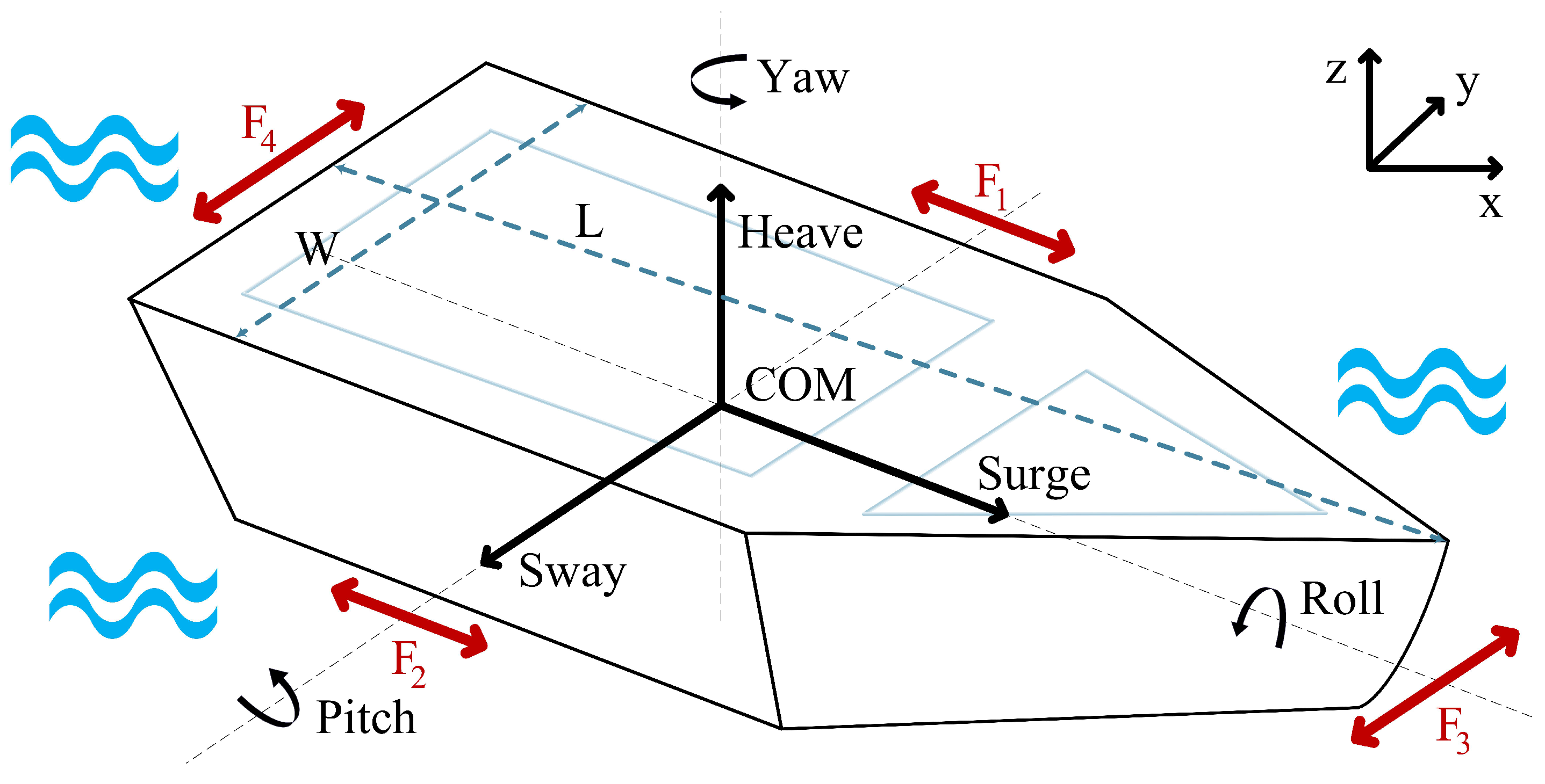
As mentioned in Section 1, this work utilizes a nonlinear USV model [41] whose schematic is given in Figure 1.

The considered USV model has a length of L, a width of W, and also four thrusters on the right, left, front, and back of the USV body. These thrusters generate the control inputs of the system, F₁, F₂, F₃, and F₄, and “COM” is short for center of mass.

Furthermore, the model has a position and direction vector given by $\eta ={\left[\begin{array}{ccc}\mathbf{x}& \mathbf{y}& \psi \end{array}\right]}^{\top }$ where x, y denote the positions and ψ denotes the yaw angle (direction of the USV). The USV also has the velocity state vector given by $\nu ={\left[\begin{array}{ccc}\mathbf{u}& \mathbf{v}& \mathbf{r}\end{array}\right]}^{\top }$ where u and v denote the surge and sway velocities, respectively, and r denotes the angular velocity of the USV.

The model of the nonlinear USV consists of two parts, one of which is the kinematic model, and is given as follows:

$$\dot{\eta }=J(\eta )\nu$$

(1)

where J matrix contains the transformation terms and can be written as

$$J(\eta )=\left[\begin{array}{ccc}cos\psi & -sin\psi & 0\\ sin\psi & cos\psi & 0\\ 0& 0& 1\end{array}\right]$$

The second part of the model is the dynamical model, which is

$$M(\dot{\nu })+C(\nu )\nu +D(\nu )\nu =\tau +{\tau }_{disturbance}$$

(2)

where the M matrix contains the mass and inertia terms, C is made up of the Coriolis and centripetal terms, and D denotes the linear damping matrix. All these matrices are given as

$$M=\left[\begin{array}{ccc}m-X_{\dot{\mathbf{u}}}& 0& -m{y}_g\\ 0& m-Y_{\dot{\mathbf{v}}}& m{x}_g-Y_{\dot{\mathbf{r}}}\\ -m{y}_g& m{x}_g-N_{\dot{\mathbf{v}}}& I_{zz}-N_{\dot{\mathbf{r}}}\end{array}\right]$$

$$C=\left[\begin{array}{ccc}0& 0& -m(x_g\mathbf{r}+\mathbf{v})\\ 0& 0& -m(y_g\mathbf{r}-\mathbf{u})\\ m(x_g\mathbf{r}+\mathbf{v})& m(y_g\mathbf{r}-\mathbf{u})& 0\end{array}\right]$$

$$D=\left[\begin{array}{ccc}-X_u& 0& 0\\ 0& -Y_v& 0\\ 0& 0& -N_r\end{array}\right]$$

where m is the mass of the USV, I_zz is the inertia along the z axis, x_g, y_g are the differences between the center of mass and origin of the USV, which are assumed to be all zero. Additionally, the input torque vector is $\tau ={\left[\begin{array}{ccc}\mathbf{X}& \mathbf{Y}& \mathbf{N}\end{array}\right]}^{\top }$ where X, Y are forces along the surge and sway directions, respectively, and N is the torque exerted along the heave direction of the USV.

$$\tau =\left[\begin{array}{c}\mathbf{X}\\ \mathbf{Y}\\ \mathbf{N}\end{array}\right]=\left[\begin{array}{cccc}1& 1& 0& 0\\ 0& 0& 1& 1\\ {\displaystyle \frac{W}{2}}& -{\displaystyle \frac{W}{2}}& {\displaystyle \frac{L}{2}}& -{\displaystyle \frac{L}{2}}\end{array}\right]\left[\begin{array}{c}{F}_1\\ F_2\\ F_3\\ F_4\end{array}\right]$$

(3)

Finally, ${\tau }_{disturbance}$ represents the disturbance torques containing wind, waves, and currents of water. Also, all the inertias are assumed to be zero or ignored, except for I_zz.

Consequently, for simulation and later calculations, the equations of motion can be obtained by reformulating Equations (1) and (2), and the perturbation model is obtained as

$$\begin{array}{l}\dot{\eta }=J(\eta )\nu \\ \dot{\nu }=M^{-1}(\tau +{\tau }_{disturbance})-M^{-1}C(\nu )\nu -M^{-1}D(\nu )\nu .\end{array}$$

(4)

3. Probabilistic Nonlinear Model Predictive Control

3.1. Problem Formulation

Regarding the probabilistic linear MPC, we similarly formulate the extended probabilistic MPC. In probabilistic linear MPC, the cost function incorporates the mean values of the system states and includes a term to minimize variations in both state and control inputs. We formulated the cost function similarly, but with the consideration of the following nonlinear system equations:

$$x_{t+1}=f(x_t,u_t)+d_t,t\ge 0$$

(5)

where f(.) represents the compact form of the nonlinear equations of motion of the USV that was given in (4) but without disturbances, x is the state vector, u represents the increment control input signal (can be referred to as Δu in the literature), and d represents the disturbances caused by wind, waves and the currents with normal distribution and has either a zero or non-zero-mean value. The cost function is

$$J=J_m({\overline{x}}_t,{\overline{u}}_{t\dots t+N-1})+J_v({\mathbb{X}}_t,K_{t\dots t+N-1})$$

(6)

and this cost function’s parts can be written as

$$J_m=\sum _{i=t}^{t+N-1}\Vert {\overline{x}}_i-r_i{\Vert }_Q^2+\Vert {\overline{u}}_i{\Vert }_R^2$$

(7)

$$J_v=\sum _{i=t}^{t+N-1}trace(Q{\mathbb{X}}_i+R{\mathbb{U}}_i)$$

(8)

where ${\overline{x}}_i$ is the mean value of the system variable, ${\overline{u}}_i$ is the optimal increment control input signal, $r_i$ is the reference signal, ${\mathbb{X}}_i$ is the covariance matrix of the state vector, ${\mathbb{U}}_i$ is the covariance matrix of the control input, Q, R are the weighting matrices for the system variable and control input, respectively, and N is the prediction horizon [30,31]. In contrast to probabilistic linear MPC, this formulation allows the covariance matrix of system variables to change along all state trajectories (operating points). When we add terminal cost and constraints for stability, a cost term for obstacle avoidance, and probabilistic constraints on system variables and control input, the following probabilistic NMPC formulation is obtained:

$${\overline{J}}_m=\sum _{i=t}^{t+N-1}(\Vert {\overline{x}}_i-r_i{\Vert }_Q^2+\Vert {\overline{u}}_i{\Vert }_R^2)+\Vert {\overline{x}}_{t+N}-r_{t+N}{\Vert }_{{\overline{Q}}_1}^2+\Vert {\tilde{d}}_{t+N}{)\Vert }_{{\overline{Q}}_2}^2$$

(9)

$${\overline{J}}_v=\sum _{i=t}^{t+N-1}trace(Q{\mathbb{X}}_i+R{\mathbb{U}}_i)+trace({\overline{Q}}_1{\mathbb{X}}_{t+N})+trace({\overline{Q}}_2{D}_{t+N})$$

(10)

$${\displaystyle \underset{u}{min}{\overline{J}}_m+{\overline{J}}_v}$$

(11)

$$s.t.x_{t+1}=f(x_t,u_t)+d_t,t\ge 0$$

(12)

$$\mathbb{P}(b_r^{\top }{x}_{t+k}\ge x_r^{max})\le p_x^r,\forall k>0$$

(13)

$$\mathbb{P}(c_s^{\top }{u}_{t+k}\ge u_s^{max})\le p_u^s,\forall k\ge 0$$

(14)

$$x_{t+N}\in \Omega$$

(15)

where $\mathbb{P}(.)$ shows the probability, $b,c$ are constant vectors, $x_r^{max},u_s^{max}$ are constraint limits of the state variable and control input, $p_x,p_u$ are the violation probabilities, $\Omega$ represents the terminal region, $J_{Obstacle}$ is the obstacle avoidance cost that is obtained from the VO method, and this cost value is explained in Section 4.

3.2. Deterministic Formulation of Probabilistic Constraints

In this work, by applying successive linearization of the nonlinear USV model at every sampling instance, to deal with probabilistic constraints on system variables and control input, the method proposed by Farina et al. [30] and Magni et al. [31] that converts the probabilistic constraints to deterministic constraints for probabilistic linear MPC is utilized and extended. Since we are considering successive linearization, the constraints are updated at each sampling instance, unlike in linear MPC. The method in the mentioned papers is summarized as follows: Consider the probabilistic constraints given in (13) and (14). One can transform these probabilistic constraints into deterministic constraints using one-sided Cantelli’s inequality [30,31].

Definition 1

(Cantelli’s Inequality). Assume y is a scalar random variable with mean $\overline{y}$ and variance $\mathbb{Y}$. Then, for every $\epsilon \in {\mathbb{R}}^{+}$, it satisfies

$$\mathbb{P}(y\ge \overline{y}+\epsilon )\le {\displaystyle \frac{\mathbb{Y}}{\mathbb{Y}+\epsilon }}$$

(16)

To use this inequality, first assume that for $\delta x>0$, the following inequality holds:

$$b^{\top }\overline{x}\le x^{max}-\delta x$$

(17)

Using both this equation and Definition 1, (13) can be written as

$$\begin{array}{cc}\hfill \mathbb{P}\{b^{\top }x\ge x^{max}\}& \le \mathbb{P}\{b^{\top }x\ge b^{\top }\overline{x}+\delta x\}\hfill \\ \hfill & \le {\displaystyle \frac{b^{\top }\mathbb{X}b}{b^{\top }\mathbb{X}b+\delta x^2}}\le p_x\hfill \end{array}$$

(18)

Considering the right-hand side of the inequality above, the following inequality can be obtained:

$$b^{\top }\mathbb{X}b({\displaystyle \frac{1-p_x}{p_x}})\le \delta x^2$$

(19)

When we consider the equality (17) and (19) together, the following deterministic constraint inequality is obtained:

$$b^{\top }\overline{x}\le x^{max}-\sqrt{b^{\top }\mathbb{X}b}\sqrt{{\displaystyle \frac{1-p_x}{p_x}}}$$

(20)

The same procedure is valid for (14), so it will also yield the following result:

$$c^{\top }\overline{u}\le u^{max}-\sqrt{c^{\top }\mathbb{U}c}\sqrt{{\displaystyle \frac{1-p_u}{p_u}}}$$

(21)

4. Velocity Obstacle Method

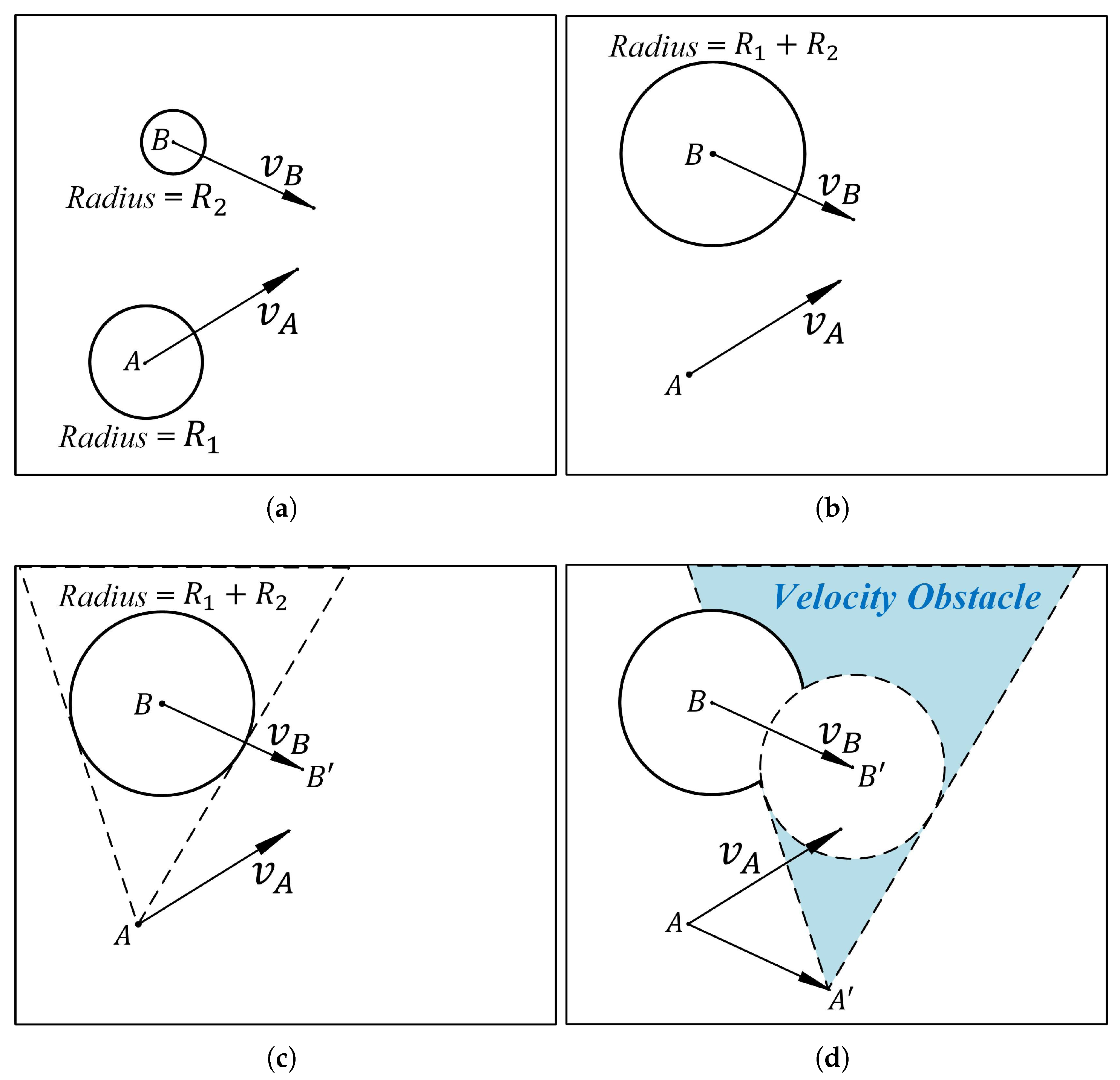
In this work, we consider the VO method for collision avoidance, which can be summarized as follows: The VO method utilizes the velocities and positions of both the ego vehicle (the main vehicle) and the obstacle vehicle to identify a collision cone defined by velocity obstacles. This technique calculates a range of possible velocities for the ego vehicle at any given moment, ensuring that it can avoid colliding with the obstacle vehicle. If the velocity of the ego vehicle falls within the collision set, the two vehicles will inevitably collide after a certain time. To illustrate this, let us consider an example of two vehicles navigating an environment. The ego vehicle has a velocity of v_A, while the obstacle vehicle travels at a velocity of v_B. Figure 2 depicts the scenario.

The collision cone is then adjusted based on the velocity of the obstacle vehicle, resulting in the creation of the “Velocity Obstacle” set. This set represents the range of velocities that the ego vehicle can take without colliding with the obstacle vehicle. If

$$v_A\notin C{C}_{A,B}\oplus v_B$$

(22)

where $C{C}_{A,B}$ is the collision cone, $C{C}_{A,B}\oplus v_B$ denotes the velocity obstacle cone, and “⊕” is the Kronecker summation symbol, the vehicle A moves without colliding with vehicle B. Therefore, a proper v_A value must be chosen. This also means that a set of positions needs to be avoided according to the time of the anticipated collision.

Let p_A be a set of positions to be avoided. This position set can be calculated as $p_A=v_A\odot t_c$, where t_c is the time to collision and “⊙” is the Kronecker product symbol. So, the obstacle cost, $J_{Obstacle}$, can be obtained as

$$J_{Obstacle}={\displaystyle \frac{K_{collision}}{x_p-p_A}}$$

(23)

where x_p denotes the first two states (N and E) of the state vector and $K_{collision}$ represents how close we can reach the outer limit of the radius of the obstacle vehicle. Also, if there is no collision possibility, $J_{Obstacle}$ is zero.

5. Proposed Control Structure

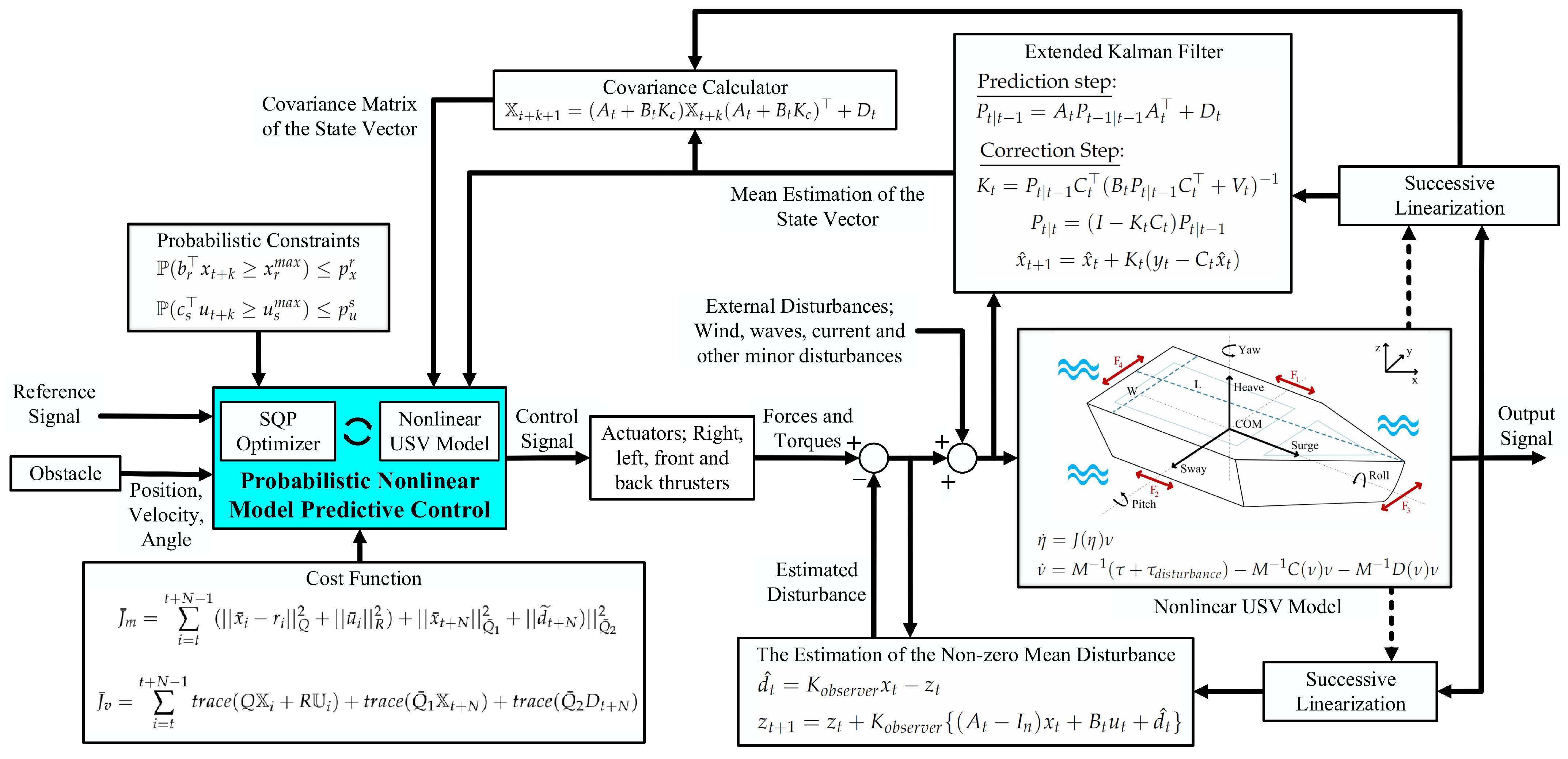
The proposed controller for the nonlinear uncrewed surface vehicle is a probabilistic NMPC that utilizes SQP as an optimizer to calculate the optimal control sequence of the control input. The cost function of the controller is designed to incorporate the mean value and covariance of the state variables, which are obtained using an EKF and a linear matrix difference equation (referred to as the covariance calculator) in the literature through successive linearization. The EKF calculates the mean value of the state vector and feeds it to the covariance calculator. The proposed controller block diagram is shown in Figure 3.

One of the unique features of this proposed controller is its ability to handle non-zero-mean disturbances, which is essential for a water-based environment where currents can exert non-zero-mean disturbances on the vehicle. To overcome this challenge, a disturbance observer is used to eliminate the effect of the non-zero-mean disturbance. We regarded the non-zero-mean disturbances as comprising both a deterministic and a probabilistic component. The deterministic component is represented by the mean of the disturbance, which is assessed using a deterministic disturbance observer. This observed mean is then sent to the MPC system to be treated as deterministic disturbances. The remaining aspect is regarded in the probabilistic MPC as a zero-mean probabilistic disturbance.

The proposed structure involves an EKF and a disturbance observer. It utilizes successive linearization to compute the mean and covariance of states and outputs, as well as to update constraints at each sampling instance and handle non-zero-mean disturbances. This proposes an extension of probabilistic linear MPC, making it applicable to nonlinear systems affected by non-zero-mean probabilistic disturbances and capable of addressing stationary and moving obstacles, essentially solving an NMPC problem. The proposed controller ensures that the vehicle can handle different scenarios with ease and can navigate through obstacles and other challenges in a water-based environment with precision.

5.1. Mean and Covariance Calculation with EKF

The Kalman filter allows for the estimation of state variable values even in noisy environments. Typically, it functions as a state observer when state measurements are absent or when outputs are noisy. Additionally, it can estimate the mean values of system states in the presence of zero-mean disturbances, even if state measurements are available. The mean value of the state vector is represented by ${\overline{x}}_{t+k|t}=\mathbb{E}\{x_{t+k|t}\}$ (estimated state). However, since USV control involves nonlinear equations of motion, an EKF [42] is necessary to estimate system states. In the EKF, the Jacobian matrices, A_t and B_t given in (24) are calculated from the nonlinear equations of motion at each sampling instance. Then, these matrices are utilized in the linear Kalman filter to determine the estimate (the mean value) of the nonlinear uncrewed surface vehicles’ state variables at that sampling instance.

$$A_t={\displaystyle \frac{\partial f(x,u)}{\partial x}}|\begin{array}{c}\hfill \begin{array}{c} \\ \\ x=x_t\\ u=u_t\end{array}\end{array},B_t={\displaystyle \frac{\partial f(x,u)}{\partial u}}|\begin{array}{c}\hfill \begin{array}{c} \\ \\ x=x_t\\ u=u_t\end{array}\end{array}$$

(24)

Namely, at each sampling instance, the nonlinear ship model is linearized around the system state variables at that time interval, as given below.

$$\begin{array}{c}{x}_{t+1}=A_t{x}_t+B_t{u}_t+d_t\end{array}$$

(25)

$$y_t=C_t{x}_t+n_t$$

(26)

Based on linearized system matrices, utilizing the following EKF steps,

• Prediction Step:

  $$\begin{array}{c}{P}_{t|t-1}=A_t{P}_{t-1|t-1}{A}_t^{\top }+D_t\end{array}$$

  (27)
• Correction Step:

  $$\begin{array}{c}{Z}_t=P_{t|t-1}{C}_t^{\top }{(B_t{P}_{t|t-1}{C}_t^{\top }+N_t)}^{-1}\end{array}$$

  (28)

  $$\begin{array}{c}{P}_{t|t}=(I-Z_t{C}_t)P_{t|t-1}\end{array}$$

  (29)

  $$\begin{array}{c}{\widehat{x}}_{t+1}={\widehat{x}}_t+Z_t(y_t-C_t{\widehat{x}}_t)\end{array}$$

  (30)

  where $D_t$ is the covariance matrix of the process noise (in our case probabilistic disturbance effect on the states), $N_t$ is the covariance matrix of the measurement noise, $Z_t$ is the Kalman gain, $P_t$ is the prediction of the covariance matrix, the estimation of the system state vector, ${\widehat{x}}_t$, under zero-mean Gaussian disturbances is obtained. Indeed, the estimated values are the mean of the state variables (${\overline{x}}_t={\widehat{x}}_t$).

After this mean calculation, the covariance matrix is calculated based on the mean state variable vector. To calculate the covariance matrix of the state variables, we utilize the following matrix equality for linear systems with successive linearization at every sampling instance [29]:

$${\mathbb{X}}_{t+k+1}={(A_t+B_t{K}_c)}^{\top }{\mathbb{X}}_{t+k}(A_t+B_t{K}_c)+D_t$$

(31)

where ${\mathbb{X}}_{t+k}=\mathbb{E}\{(x_{t+k}-{\overline{x}}_{t+k}){(x_{t+k}-{\overline{x}}_{t+k})}^{\top }\}$, and $K_c$ is the control gain. It can be represented as $K_{MPC}$, which is the MPC control gain calculated with SQP optimization at every time instant before the prediction horizon, and then it takes the form of $K_{LQG}$, which is the linear quadratic Gaussian (LQG) control gain, and is calculated at the end of the prediction horizon. For the calculation of covariance in Equation (31), the mean value of the state vector is required, where we obtain it using an EKF.

5.2. Estimation of the Mean of the Non-Zero-Mean Disturbance

A novel aspect of this work addresses non-zero-mean disturbances by treating them as a combination of deterministic and probabilistic parts. The mean of the non-zero-mean probabilistic disturbance, as a novel approach, is assumed to be the deterministic part, which we propose to observe using a deterministic disturbance observer. Therefore, to estimate the deterministic part of the disturbances, a linear disturbance observer is integrated into the proposed control structure. The disturbance observer given in the following is adopted based on the linear system model at (25) and (26). The disturbance observer utilized is [43]

$$\begin{array}{c}{\widehat{d}}_t=K_{OB}{x}_t-z_t\hfill \end{array}$$

(32)

$$\begin{array}{c}{z}_{t+1}=z_t+K_{OB}\{(A_t-I_n)x_t+B_t{u}_t+{\widehat{d}}_t\}\hfill \end{array}$$

(33)

where ${\widehat{d}}_t$ is the estimated deterministic part of the disturbance; $d_t$, $z_t$ is the state variable of the disturbance observer, and $K_{OB}$ is the gain matrix of the observer.

6. Feasibility and Stability Analysis

In order to ensure the stability of the considered controller system, a dual-mode strategy is considered. After the prediction horizon, an LQG controller that guarantees the stability under the effect of the non-zero mean stochastic disturbance (its mean is considered as deterministic disturbance and the remaining part as zero-mean Gaussian disturbance), $u_t=-K_t{x}_t-{(B_t^{\top }{B}_t)}^{-1}{B}_t^{\top }{\widehat{d}}_t$, is utilized where we normally minimize the tracking error, where $K_t$ is the general representation of the feedback control gain, and for stability analysis, $x_t$ is the tracking error for the general notation.

To start, we need to verify the feasibility of the controller system. Assume that, for $u_{LQG}=-K_{LQG}{x}_t-{(B_t^{\top }{B}_t)}^{-1}{B}_t^{\top }{\widehat{d}}_t$, the closed-loop system is stable in $\Omega$, satisfying constraints (20) and (21), and $\Omega$ is invariant under the $u_{LQG}$ control law (see Appendix A). If the MPC problem is feasible at time t, $x_{t+N}$ in $\Omega$, then this implies that the optimization problem is feasible at time $t+1$ based on the following analysis.

Note that $x_{t+N}:({\overline{x}}_{t+N},{\mathbb{X}}_{t+N})\in \Omega ({\Omega }_m,{\Omega }_v)$, where $A_K\overline{x}\in {\Omega }_m$, in which $A_K$ is the closed-loop system matrix of the dual-mode control obtained with LQG, and ${\mathbb{X}}_{t+N}\le \overline{\mathbb{X}}\in {\Omega }_v$. $\overline{\mathbb{X}}$ is the steady-state solution of (31) with noise variance $\overline{D}>D$, namely $\overline{\mathbb{X}}=A_K^{\top }\overline{\mathbb{X}}{A}_K+\overline{D}$.

Owing to invariant property of $\Omega$ under LQG control,

$${\overline{x}}_{t+N+1}=A_{t+N}{\overline{x}}_{t+N}+B_{t+N}{\overline{u}}_{LQG}\in {\Omega }_m$$

(34)

$$\overline{u}=-K_{LQG}\overline{x}-{(B_t^{\top }{B}_t)}^{-1}{B}_t^{\top }{\widehat{d}}_t$$

(35)

is valid, and because of the Gaussian white noise acting on the system, one can state that

$${\mathbb{X}}_{t+N+1}=A_K^{\top }{\mathbb{X}}_{t+N}{A}_K+D_{t+N}\le \overline{\mathbb{X}}=A_K^{\top }\overline{\mathbb{X}}{A}_K+\overline{D}$$

(36)

Therefore, the pair $({\overline{x}}_{t+N+1},{\mathbb{X}}_{t+N+1})$ is also in $\Omega$. We can conclude that the optimization problem is also feasible at time $t+N+1$. Also, one can say, if we choose $t+N$ as any value, this feasibility statement is valid for any time instant, leading to recursive feasibility.

After verifying recursive feasibility, stability analysis can be performed as follows: For this purpose, the cost of mode 2 (LQG) is added as a terminal cost to the finite-horizon cost to obtain infinite-horizon cost, so that the obtained infinite-horizon cost can be considered as a Lyapunov function for the considered closed-loop system obtained with dual-mode MPC and LQG control. A final constraint, as the terminal region $\Omega$, is also added to the MPC formulation to ensure system states converge to an invariant set of LQG control. LQG ensures that once the system states enter the terminal region, they remain in the region.

Recalling the problem formulation which is given in Equations (9)–(15), we then consider the following infinite-horizon cost, obtained by adding the infinite-time state trajectory cost after the prediction horizon to the finite-horizon cost:

$${\overline{J}}_m=\sum _{i=t}^{t+N-1}(\Vert {\overline{x}}_i{\Vert }_Q^2+\Vert {\overline{u}}_i{\Vert }_R^2)+\sum _{i=t+N}^{\infty }(\Vert {\overline{x}}_i{\Vert }_Q^2)$$

(37)

$${\overline{J}}_v=\sum _{i=t}^{t+N-1}trace(Q{\mathbb{X}}_i+R{\mathbb{U}}_i)+\sum _{i=t+N}^{\infty }trace(Q{\mathbb{X}}_i)$$

(38)

Now, we calculate the sum of all the output values of the system from the end of the prediction horizon to infinity. Then, we can write down $x_{t+N+i}$ values for $i=0,1,2,3,\dots$ and obtain

$$\begin{array}{l}{\overline{x}}_{t+N}={\overline{x}}_{t+N}\\ {\overline{x}}_{t+N+1}=A_K{\overline{x}}_{t+N}+{\tilde{d}}_{t+N}\\ {\overline{x}}_{t+N+2}=A_K(A_K{\overline{x}}_{t+N}+{\tilde{d}}_{t+N})+{\tilde{d}}_{t+N+1}=A_K^2{\overline{x}}_{t+N}+A_K{\tilde{d}}_{t+N}+{\tilde{d}}_{t+N+1}\\ \dots \\ {\overline{x}}_{t+N+j}=A_K^j{\overline{x}}_{t+N}+A_K^{j-1}{\tilde{d}}_{t+N}+A_K^{j-2}{\tilde{d}}_{t+N+1}+\dots +A_K{\tilde{d}}_{t+N+j-2}+{\tilde{d}}_{t+N+j-1}\end{array}$$

where ${\widehat{d}}_t$ is the predicted mean value of the disturbance $d_t$, and $\tilde{d}$ is the remaining zero-mean stochastic disturbance. And now, the next step is to calculate the ${\tilde{d}}_{t+1}$ term by looking into disturbance observer Equations (32) and (33).

$$\begin{array}{cc}\hfill {\widehat{d}}_{t+1}& =K_{OB}{x}_{t+1}-z_{t+1}\hfill \\ \hfill & =K_{OB}(A_K{x}_t+{\tilde{d}}_t)-(z_t+K_{OB}(A_t-x_t+B_t{u}_t+{\widehat{d}}_t))\hfill \\ \hfill & =K_{OB}{A}_K{x}_t+K_{OB}{\tilde{d}}_t+{\widehat{d}}_t-K_{OB}{A}_t{x}_t+K_{OB}{B}_t{K}_t{x}_t+K_{OB}{\widehat{d}}_t-K_{OB}{\widehat{d}}_t\hfill \\ \hfill & =K_{OB}{\tilde{d}}_t+{\widehat{d}}_t\hfill \end{array}$$

(39)

From here, using two equalities for the disturbance, ${\tilde{d}}_t={\overline{d}}_t-{\widehat{d}}_t$ and ${\overline{d}}_{t+1}={\overline{d}}_t$, we obtain

$$\begin{array}{c}{\tilde{d}}_{t+1}={\overline{d}}_{t+1}-(K_{OB}{\tilde{d}}_t+{\widehat{d}}_t)\hfill \\ {\tilde{d}}_{t+1}={\overline{d}}_t-K_{OB}{\tilde{d}}_t-{\widehat{d}}_t\hfill \end{array}$$

(40)

This yields

$${\tilde{d}}_{t+1}={\tilde{d}}_t-K_{OB}{\tilde{d}}_t$$

(41)

Considering any $jth$ equation of the above prediction equations and the disturbance observer equality we obtained in (41), we can rewrite the equation as

$$\begin{array}{cc}\hfill {\overline{x}}_{t+N+j}=& A_K^j{\overline{x}}_{t+N}+A_K^{j-1}{\tilde{d}}_{t+N}+A_K^{j-2}(1-K_{OB}){\tilde{d}}_{t+N}+A_K^{j-3}{(1-K_{OB})}^2{\tilde{d}}_{t+N}+\dots \hfill \\ \hfill & +A_K{(1-K_{OB})}^{j-2}{\tilde{d}}_{t+N}+{(1-K_{OB})}^{j-1}{\tilde{d}}_{t+N}\hfill \end{array}$$

(42)

and this summation can be written as

$${\overline{x}}_{t+N+j}=A_K^j{\overline{x}}_{t+N}+\sum _{i=0}^{j-1}{A}_K^{j-1-i}{(1-K_{OB})}^i{\tilde{d}}_{t+N}$$

(43)

Now we can say that $A_K^j=\tilde{A}$ and ${\sum }_{i=0}^{j-1}{A}_K^{j-1-i}{(1-K_{OB})}^i=\check{A}$, and so (43) becomes

$${\overline{x}}_{t+N+j}=\tilde{A}{\overline{x}}_{t+N}+\check{A}{\tilde{d}}_{t+N}$$

(44)

Starting from $t+N$, as j goes to infinity, the infinite-horizon trajectory tracking cost can be written as follows:

$$\begin{array}{cc}\hfill \sum _{i=t+N}^{\infty }\Vert {\overline{x}}_i{\Vert }_Q=& {\overline{x}}_{t+N}^{\top }[\sum _{i=0}^{\infty }{({\tilde{A}}^{\top })}^{i}Q{(\tilde{A})}^i]{\overline{x}}_{t+N}+2{\overline{x}}_{t+N}^{\top }[\sum _{i=0}^{\infty }{({\tilde{A}}^{\top })}^{i}Q{(\check{A})}^i]{\tilde{d}}_{t+N}\hfill \\ \hfill & +{\tilde{d}}_{t+N}^{\top }[\sum _{i=0}^{\infty }{({\check{A}}^{\top })}^{i}Q{(\check{A})}^i]{\tilde{d}}_{t+N}\hfill \end{array}$$

(45)

After this step, we can use the Young inequality on the second term with coefficient ${\gamma }_1\in {\mathbb{R}}^{+}$ and obtain

$$\sum _{i=t+N}^{\infty }\Vert {\overline{x}}_i{\left|\right|}_Q\le (1+{\gamma }_1){\overline{x}}_{t+N}^{\top }[\sum _{i=0}^{\infty }{({\tilde{A}}^{\top })}^{i}Q{(\tilde{A})}^i]{\overline{x}}_{t+N}+(1+{\displaystyle \frac{1}{{\gamma }_1}}){\tilde{d}}_{t+N}^{\top }[\sum _{i=0}^{\infty }{({\check{A}}^{\top })}^{i}Q{(\check{A})}^i]{\tilde{d}}_{t+N}$$

(46)

Now, we are making the following assignments to obtain the terminal cost weight matrices

$${\overline{Q}}_1=(1+{\gamma }_1)[\sum _{i=0}^{\infty }{({\tilde{A}}^{\top })}^{i}Q{(\tilde{A})}^i]{\overline{x}}_{t+N}$$

(47)

$${\overline{Q}}_2=(1+{\displaystyle \frac{1}{{\gamma }_1}})[\sum _{i=0}^{\infty }{({\check{A}}^{\top })}^{i}Q{(\check{A})}^i]{\tilde{d}}_{t+N}$$

(48)

From these matrices, we can write the following compact formulation for the cost as

$$\sum _{i=N+1}^{\infty }\Vert {\overline{x}}_{t+i}{\Vert }_Q\le {\overline{x}}_{t+N}^{\top }{\overline{Q}}_1{\overline{x}}_{t+N}+{\tilde{d}}_{t+N}^{\top }{\overline{Q}}_2{\tilde{d}}_{t+N}$$

(49)

Similarly, we can calculate $trace({\mathbb{X}}_{t+N+i})$ values for $i=0,1,2,3,\dots$ using almost the same procedure as above while using the properties of the trace: $tr(A+B)=tr(A)+tr(B),tr(AB)=tr(BA)$

$$\begin{array}{c}trace({\mathbb{X}}_{t+N})=trace({\mathbb{X}}_{t+N})\hfill \\ trace({\mathbb{X}}_{t+N+1})=trace(A_K^{\top }{\mathbb{X}}_{t+N}{A}_K+D_{t+N})\hfill \\ trace({\mathbb{X}}_{t+N+2})=trace({(A_K^2)}^{\top }{\mathbb{X}}_{t+N}(A_K^2)+A_K^{\top }{D}_{t+N}{A}_K+D_{t+N})\hfill \\ \dots \hfill \\ \begin{array}{l}trace({\mathbb{X}}_{t+N+j})=trace({(A_K^j)}^{\top }{\mathbb{X}}_{t+N}(A_K^j)+{(A^{j-1})}_K^{\top }{D}_{t+N}{A}_K^{j-1}\\ +{(A_K^{j-2})}^{\top }{D}_{t+N+1}{A}_K^{j-2}+\dots +A_K^{\top }{D}_{t+N+j-2}{A}_K+D_{t+N+j-1})\end{array}\hfill \end{array}$$

In a compact form, it can be rewritten as

$$trace({\mathbb{X}}_{t+N+j})=trace({(A_K^j)}^{\top }{\mathbb{X}}_{t+N}{A}_K^j+\sum _{i=0}^{j-1}{(A_K^{j-1-i})}^{\top }{(1-K_{OB})}^i{D}_{t+N}{A}_K^{j-1-i})$$

(50)

If we follow the similar steps like in Equations (44) to (48), the summation (50) leads to

$$\sum _{i=N+1}^{\infty }trace(Q{\mathbb{X}}_i)=trace({\overline{Q}}_1{\mathbb{X}}_{t+N})+trace({\overline{Q}}_2{D}_{t+N})$$

(51)

So, the objective functions $J_m$ and $J_v$ in Equations (37) and (38) become as in Equations (9) and (10). In the next phase, we need to calculate $V_{t+1}-V_t$, where $V_t=x_t^{\top }{\overline{Q}}_1{x}_t+{\tilde{d}}_t^{\top }{\overline{Q}}_2{\tilde{d}}_t$. So,

$$V_{t+1}-V_t=x_{t+1}^{\top }{\overline{Q}}_1{x}_{t+1}-x_t^{\top }{\overline{Q}}_1{x}_t+{\tilde{d}}_{t+1}^{\top }{\overline{Q}}_2{\tilde{d}}_{t+1}-{\tilde{d}}_t^{\top }{\overline{Q}}_2{\tilde{d}}_t$$

(52)

$$\begin{array}{cc}\hfill x_{t+1}^{\top }{\overline{Q}}_1{x}_{t+1}& ={(A_K{x}_t+{\tilde{d}}_t)}^{\top }{\overline{Q}}_1(A_K{x}_t+{\tilde{d}}_t)\hfill \\ \hfill & =x_t^{\top }{A}_K^{\top }{\overline{Q}}_1{A}_K{x}_t+2x_t^{\top }{A}_K^{\top }{\overline{Q}}_1{\tilde{d}}_t+{\tilde{d}}_t^{\top }{\overline{Q}}_1{\tilde{d}}_t\hfill \end{array}$$

(53)

$$\begin{array}{cc}\hfill {\tilde{d}}_{t+1}^{\top }{\overline{Q}}_2{\tilde{d}}_{t+1}& ={({\tilde{d}}_t-K_{OB}{\tilde{d}}_t)}^{\top }{\overline{Q}}_2({\tilde{d}}_t-K_{OB}{\tilde{d}}_t)\hfill \\ \hfill & ={(1-K_{OB})}^2{\tilde{d}}_t^{\top }{\overline{Q}}_2{\tilde{d}}_t\hfill \end{array}$$

(54)

In view of these equations, we can write

$$\begin{array}{cc}\hfill V_{t+1}-V_t=& x_t^{\top }{A}_K^{\top }{\overline{Q}}_1{A}_K{x}_t+2x_t^{\top }{A}_K^{\top }{\overline{Q}}_1{\tilde{d}}_t+{\tilde{d}}_t^{\top }{\overline{Q}}_1{\tilde{d}}_t-x_t^{\top }{\overline{Q}}_1{x}_t\hfill \\ \hfill & +{(1-K_{OB})}^2{\tilde{d}}_t^{\top }{\overline{Q}}_2{\tilde{d}}_t-{\tilde{d}}_t^{\top }{\overline{Q}}_2{\tilde{d}}_t\hfill \end{array}$$

(55)

Using the Young inequality again in $2x_t^{\top }{A}_K^{\top }{\overline{Q}}_1{\tilde{d}}_t$ with a coefficient of ${\gamma }_2\in {\mathbb{R}}^{+}$, we obtain

$$\begin{array}{cc}\hfill V_{t+1}-V_t\le & -x_t^{\top }{\overline{Q}}_1{x}_t+(1+{\gamma }_2)x_t^{\top }{A}_K^{\top }{\overline{Q}}_1{A}_K{x}_t+(1+{\displaystyle \frac{1}{{\gamma }_2}}){\tilde{d}}_t^{\top }{\overline{Q}}_1{\tilde{d}}_t\hfill \\ \hfill & +(K_{OB}^2-2K_{OB}){\tilde{d}}_t^{\top }{\overline{Q}}_2{\tilde{d}}_t\hfill \end{array}$$

(56)

At this point, to guarantee the stability, the following equality should hold:

$$V_{t+1}-V_t=-x_t^{\top }Q{x}_t-u_t^{\top }R{u}_t$$

(57)

We implement $u_t=-K_t{x}_t-{(B_t^{\top }{B}_t)}^{-1}{B}_t^{\top }{\widehat{d}}_t$ and use the Young inequality again for the right-hand side of the equality (56) with the coefficient of ${\gamma }_3\in {\mathbb{R}}^{+}$. Therefore, one can obtain

$$\begin{array}{cc}\hfill x_t^{\top }{\overline{Q}}_1{x}_t+{\tilde{d}}_t^{\top }{\overline{Q}}_2{\tilde{d}}_t-& (1+{\gamma }_2)x_t^{\top }{A}_K^{\top }{\overline{Q}}_1{A}_K{x}_t-(1+{\displaystyle \frac{1}{{\gamma }_2}}){\tilde{d}}_t^{\top }{\overline{Q}}_1{\tilde{d}}_t+(K_{OB}^2-2K_{OB}){\tilde{d}}_t^{\top }{\overline{Q}}_2{\tilde{d}}_t\hfill \\ & \ge (1+{\gamma }_3)x_t^{\top }{K}_{LQG}^{\top }R{K}_{LQG}{x}_t+(1+{\displaystyle \frac{1}{{\gamma }_3}}){\widehat{d}}_t^{\top }{L}_t^{\top }R{L}_t{\widehat{d}}_t+x_t^{\top }Q{x}_t\hfill \end{array}$$

(58)

where $L_t={(B_t^{\top }{B}_t)}^{-1}{B}_t^{\top }$, and the equation above yields the following Riccati inequalities:

$${\overline{Q}}_1-(1+{\gamma }_2)A_K^{\top }{\overline{Q}}_1{A}_K\ge (1+{\gamma }_3)K_{LQG}^{\top }R{K}_{LQG}+Q$$

(59)

$$(2K_{OB}-K_{OB}^2){\overline{Q}}_2-(1+{\displaystyle \frac{1}{{\gamma }_2}}){\overline{Q}}_1\ge (1+{\displaystyle \frac{1}{{\gamma }_3}})L_t^{\top }R{L}_t$$

(60)

For chosen Q and R matrices, ${\overline{Q}}_1$ and ${\overline{Q}}_2$ can be calculated.

To show the convergence of the output of the system, we need to show that $J^{\ast }(t+1)-J^{\ast }(t)\le 0$, where $J^{\ast }(t)$ is the Lyapunov function and can be denoted as $J^{\ast }(t)=J_m^{\ast }(t)+J_v^{\ast }(t)$, where $J_m(.)$ and $J_v(.)$ are mean and covariance parts of the Lyapunov function. For the first part of this Lyapunov function, we can write

$$\begin{array}{cc}\hfill J_m^{\ast }(t+1)=& J_m^{\ast }(t)-\Vert {\overline{x}}_{t|t}{\Vert }_Q^2-\Vert {\overline{u}}_{t|t}{\Vert }_R^2+\Vert {\overline{x}}_{t+N|t}{\Vert }_Q^2+\Vert K_{LQG}{\overline{x}}_{t+N|t}{\Vert }_R^2\hfill \\ \hfill & +\Vert L_{t+N}{\widehat{d}}_{t+N}{\Vert }_R^2-\Vert {\overline{x}}_{t+N|t}{\Vert }_{{\overline{Q}}_1}^2+\Vert (A+B{K}_{LQG}){\overline{x}}_{t+N|t}{\Vert }_{{\overline{Q}}_1}^2\hfill \end{array}$$

(61)

Now, in view of (59), we can obtain

$$\begin{array}{cc}\hfill J_m^{\ast }(t+1)-J_m^{\ast }(t)\le & -\mathbb{E}\{\Vert x_t{\Vert }_Q^2+\Vert u_t{\Vert }_R^2\}-{\gamma }_3\Vert K_{LQG}{\overline{x}}_{t+N|t}{\Vert }_R^2\hfill \\ \hfill & -{\gamma }_2\Vert (A+B{K}_{LQG}){\overline{x}}_{t+N|t}{\Vert }_{{\overline{Q}}_1}^2\hfill \end{array}$$

(62)

For this inequality, we can say

$$J_m^{\ast }(t+1)-J_m^{\ast }(t)<-\mathbb{E}\{\Vert x_t{\Vert }_Q^2+\Vert u_t{\Vert }_R^2\}$$

(63)

Also, for the second part of the Lyapunov function

$$\begin{array}{cc}\hfill J_v^{\ast }(t+1)=& J_v^{\ast }(t)-tr\{(Q+K_{MPC}^{\top }R{K}_{MPC}){\mathbb{X}}_t\}+tr\{(Q+K_{LQG}^{\top }R{K}_{LQG}){\mathbb{X}}_{t+N}\hfill \\ \hfill & +{\overline{Q}}_1{(A+B{K}_{LQG})}^{\top }{\mathbb{X}}_{t+N}(A+B{K}_{LQG})+{\overline{Q}}_{1}D-{\overline{Q}}_1{\mathbb{X}}_{t+N}\}\hfill \end{array}$$

(64)

where $K_{LQG}$ is the gain calculated from the LQ problem. Now, using properties of the trace again and in view of (59), we can write

$$\begin{array}{cc}\hfill & tr\{(Q+K_{LQG}^{\top }R{K}_{LQG}){\mathbb{X}}_{t+N}+{\overline{Q}}_1{(A+B{K}_{LQG})}^{\top }{\mathbb{X}}_{t+N}(A+B{K}_{LQG})\}\hfill \\ \hfill & =tr\{[(Q+K_{LQG}^{\top }R{K}_{LQG})+{\overline{Q}}_1{(A+B{K}_{LQG})}^{\top }(A+B{K}_{LQG})]{\mathbb{X}}_{t+N}\}\hfill \\ \hfill & \le tr\{-{\gamma }_3{K}_{LQG}^{\top }R{K}_{LQG}{\mathbb{X}}_{t+N}-{\gamma }_2(A+B{K}_{LQG}){\mathbb{X}}_{t+N}+{\overline{Q}}_1{\mathbb{X}}_{t+N}\}\hfill \end{array}$$

(65)

In view of this little manipulation, (64) becomes

$$J_v^{\ast }(t+1)-J_v^{\ast }(t)\le tr\{{\overline{Q}}_{1}D-{\gamma }_3{K}_{LQG}^{\top }R{K}_{LQG}{\mathbb{X}}_{t+N}-{\gamma }_2(A+B{K}_{LQG}){\mathbb{X}}_{t+N}\}$$

(66)

Then, we can say

$$J_v^{\ast }(t+1)-J_v^{\ast }(t)<tr\{{\overline{Q}}_{1}D\}$$

(67)

As a result, we can put together Equations (63) and (67), which yields the following inequality:

$$J^{\ast }(t+1)-J^{\ast }(t)<-\mathbb{E}\{\Vert x_t{\Vert }_Q^2+\Vert u_t{\Vert }_R^2\}+tr\{{\overline{Q}}_{1}D\}$$

(68)

The inequality (68) is the same as the equality (32) in the study [30]. This proves $J^{\ast }(t+1)-J^{\ast }(t)<0$ is very similar to the proof in [30]. Therefore, we do not need to repeat the proof here, and the stability proof is completed.

7. Simulation and Results

In this section, we present the simulation results. To demonstrate the positive effects of the proposed controller on tracking performance, a simulation was carried out using the Simulink and Optimization toolboxes in the 2023a version of MATLAB^®.

In our simulation, we employ SQP to solve the formulated NMPC problem. SQP is a robust optimization method specifically designed for constrained nonlinear optimization problems [44,45]. This method effectively handles both initial and dynamic constraints, as well as various equality constraints. It is particularly adept at finding optimal solutions for complex nonlinear systems.

First of all, we need to allocate the system parameters to the simulation, which are given in

Table 1. Model parameters for the considered controller system.

Parameter	Value	Unit	Parameter	Value	Unit
m	15	kg	$Y_{\mathbf{v}}$	10	kg/s
W	0.5	m	$N_{\mathbf{r}}$	2	kg·m2/rad·s
L	1	m	$X_{\dot{\mathbf{u}}}$	−1	kg
Izz	5	kg· m2	$Y_{\dot{\mathbf{v}}}$	−10	kg
Xu	5	kg/s	$N_{\dot{\mathbf{r}}}$	−4	kg· m2

below.

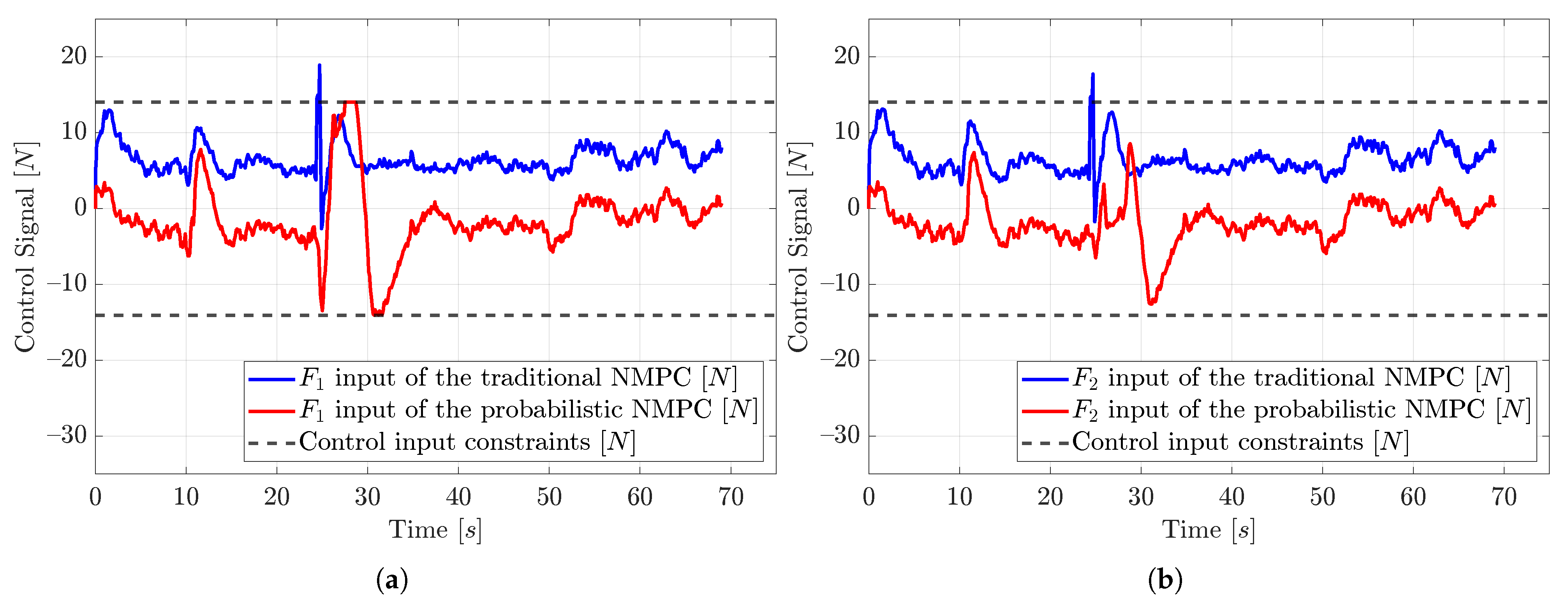
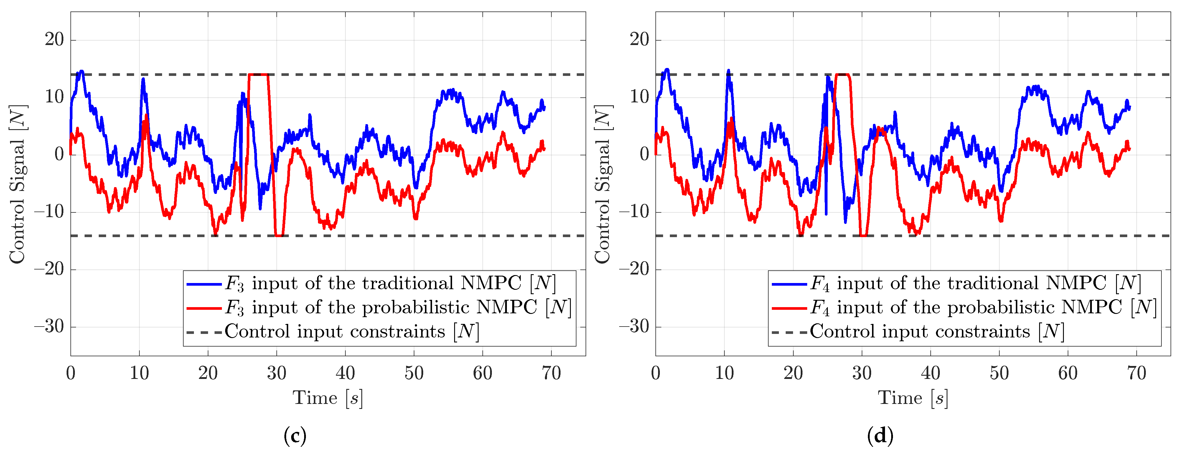
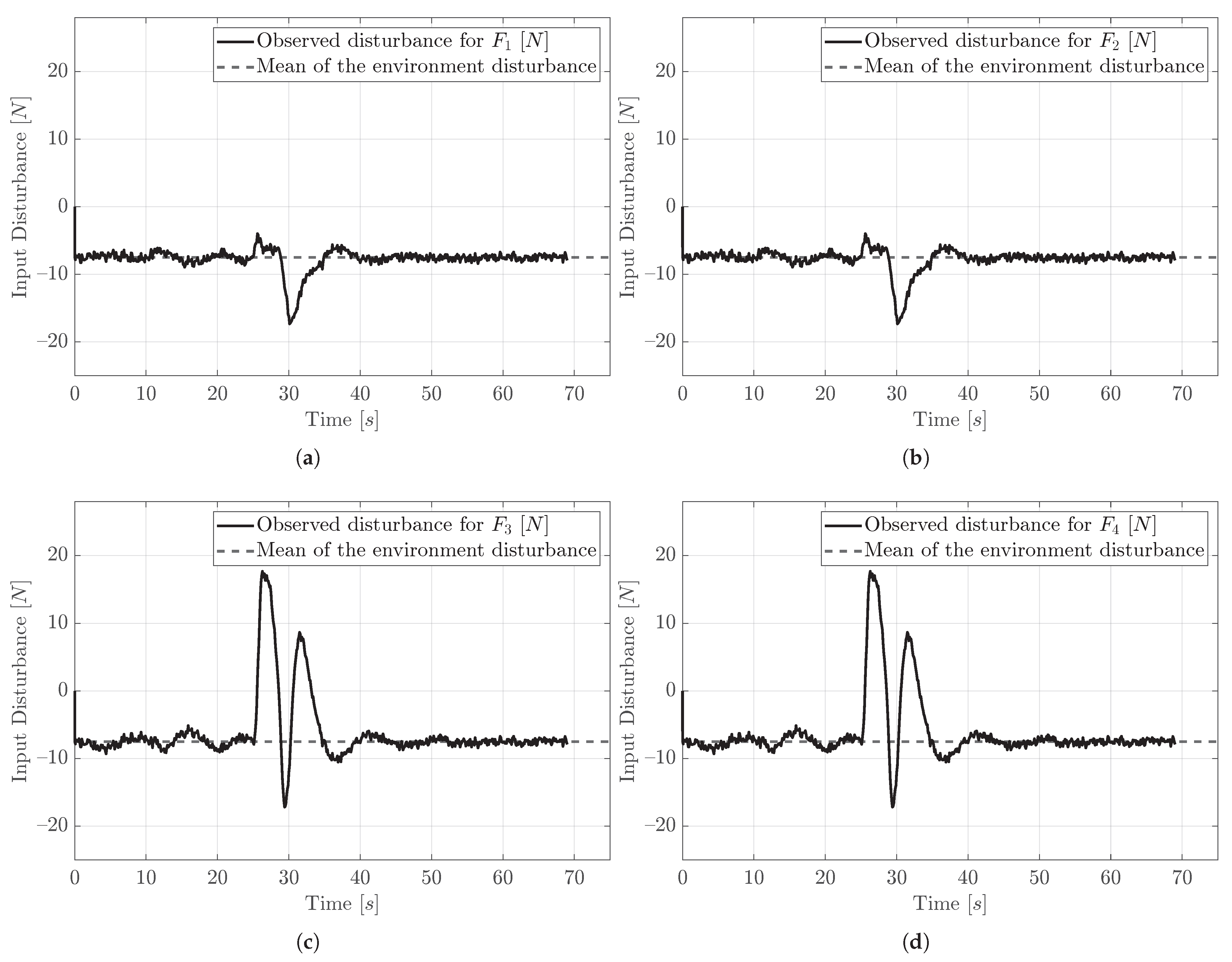
Now, we need to specify the disturbances acting on the system and other parameters. The disturbance forces acting on the system inputs have Gaussian white noise with a variance value of 0.1. However, the mean value of these disturbance forces is −7.5 N for all control inputs, $F_1$, $F_2$,$F_3$, and $F_4$, and there is no torque disturbance because the considered disturbance is only the current of the water.

Normally, the control input constraints without probabilistic effects are chosen as $-15\mathrm{N}\le u\le 15\mathrm{N}$. However, if we take the probabilistic effects into account and calculate the probabilistic constraints described in (20) and (21) in which $b_r$, $c_s$ are both chosen as 1 and $p_u$ is chosen as 0.1, the control input constraints become $-14.051312\mathrm{N}\le u\le 14.051312\mathrm{N}$.

Weight matrices in the cost function are selected as $Q=100I_{3\times 3}$ and $R=0.1I_{4\times 4}$, and the terminal weight matrix ${\overline{Q}}_1$ is the calculated from (59). Additionally, for the moving obstacle, $K_{collision}=3$, for the stationary obstacle, $K_{collision}=6$, and for the observer, $K_{OB}=0.7$.

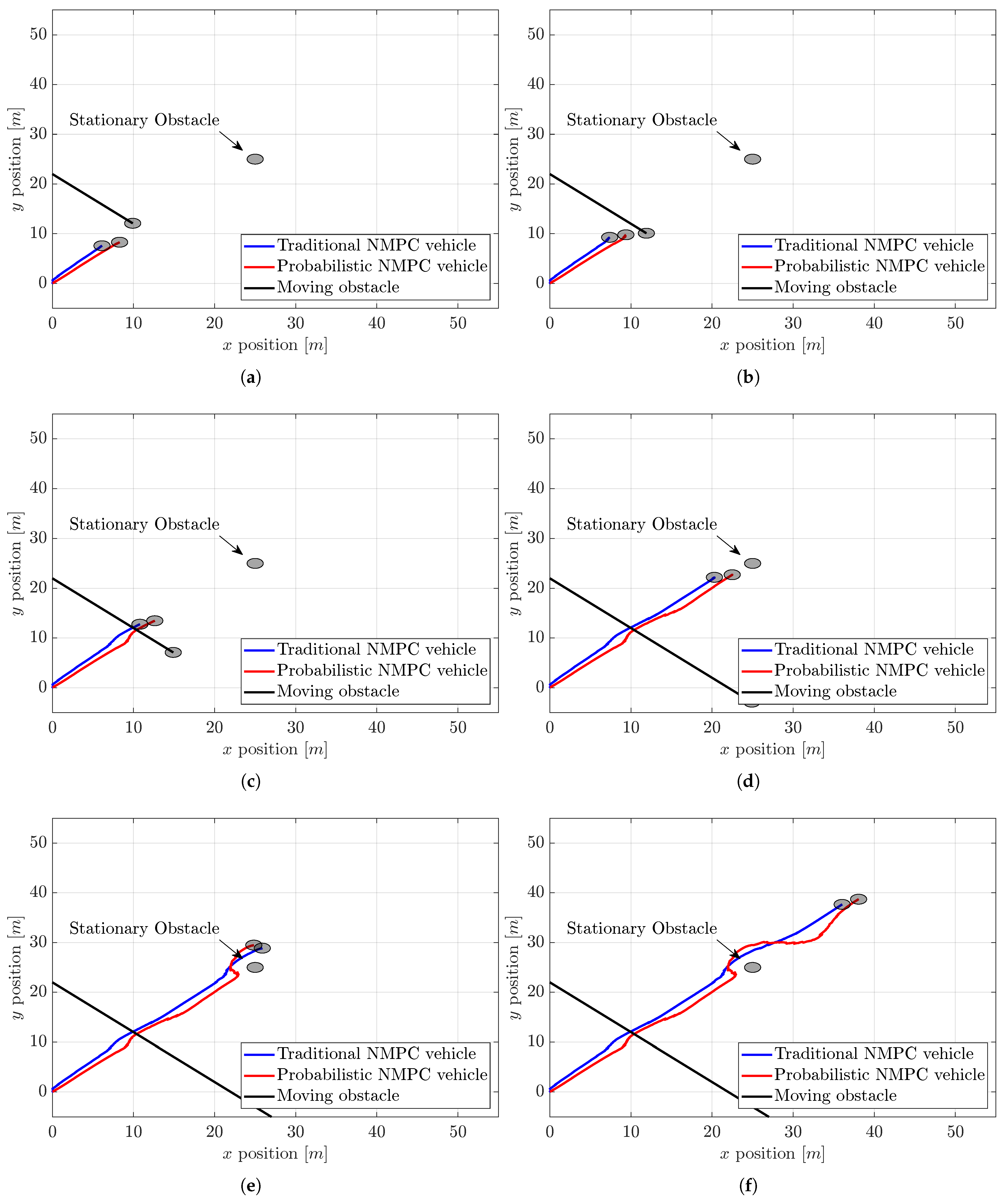
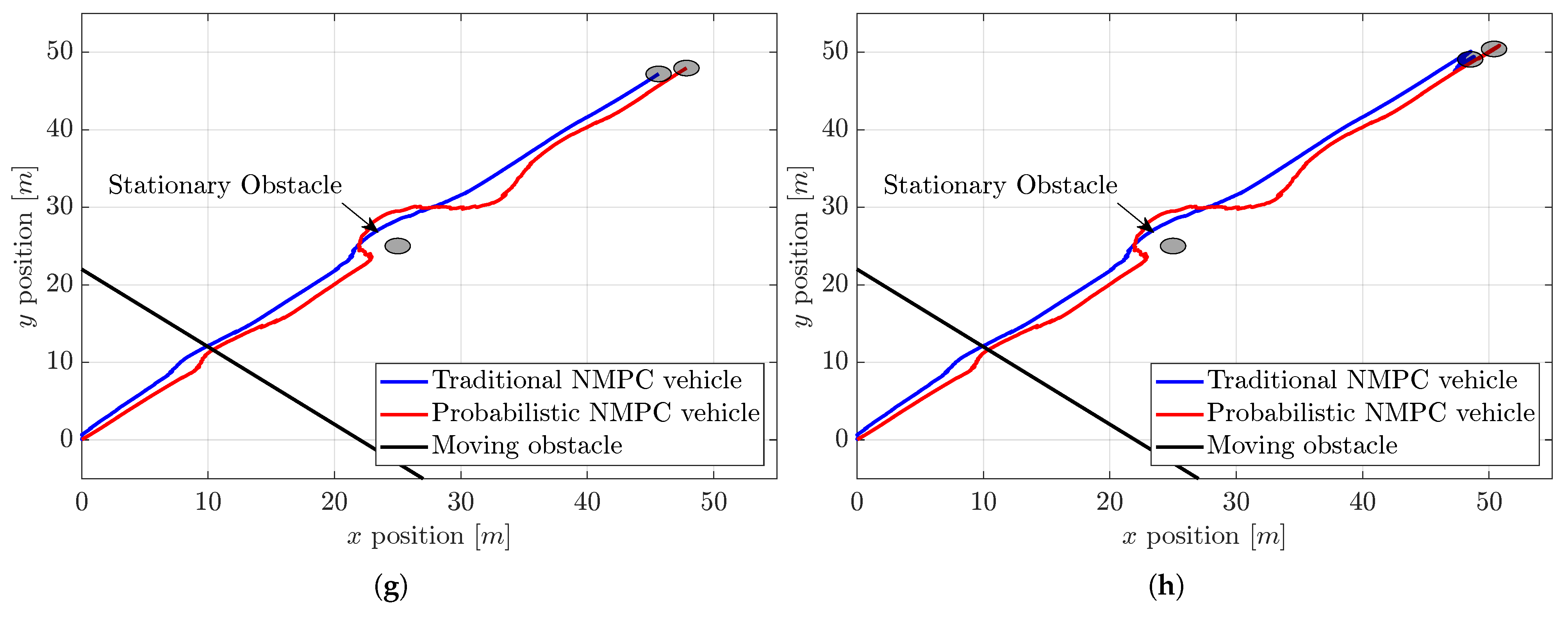
In Figure 4, we illustrate the tracking and obstacle avoidance performance of traditional NMPC compared to the proposed probabilistic NMPC with obstacles and stochastic disturbances. When we say traditional NPMC, it means that the control system has no disturbance observer, no EKF, or no probabilistic effects taken into account in optimization. Also, it is important to stress that an invisible straight line from (0 m, 0 m) point to (50 m, 50 m) point is our reference path in this study; namely, we consider a ramp reference. Simulations are performed with a sampling time of 0.1 s.

Upon examining Figure 4, in view of negative values of the disturbance, the traditional NMPC vehicle tracks the reference path slightly to the left and behind the vehicle managed by the probabilistic NMPC. Both vehicles encounter the moving obstacle between 11 and 12 s, navigating past this obstacle quite closely, as the collision gain for this situation is small. Nonetheless, when both vehicles confront the stationary obstacle around 26 to 27 s, they diverge more to avoid it due to the increased collision gain associated with this obstacle. During this avoidance maneuver, the vehicle operated by traditional NMPC does not have to change its position much, as it is already situated to the left of the desired trajectory. But the probabilistic one needs more maneuvering because it is situated almost on the trajectory. And then, both vehicles arrive at their final position around the coordinates (50 m, 50 m).

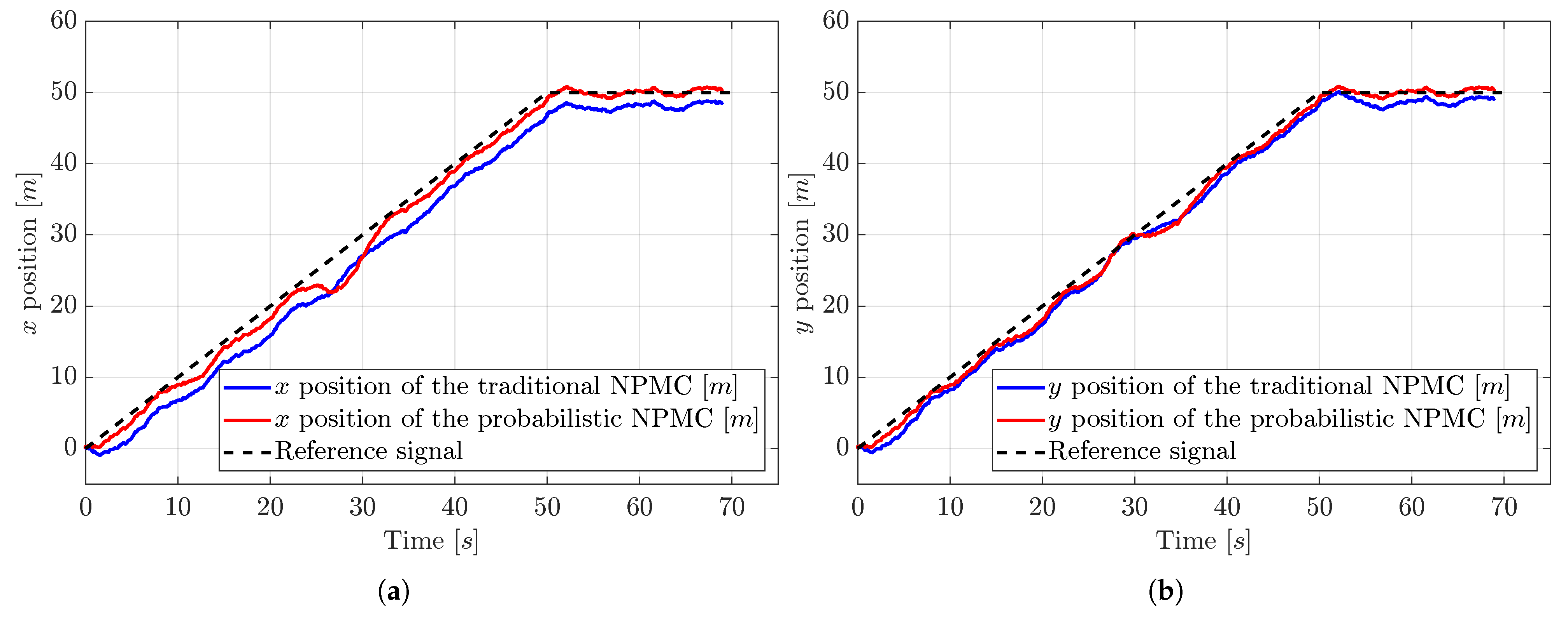
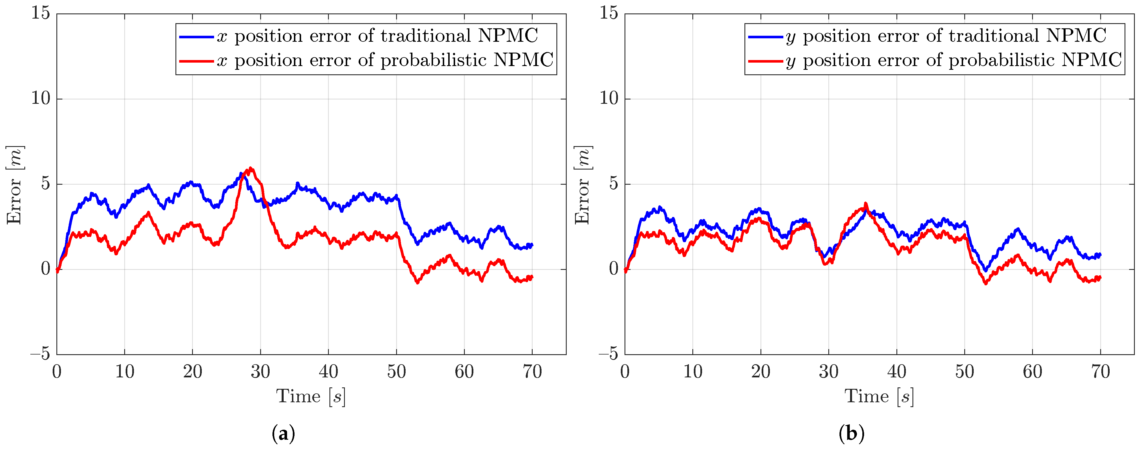
While tracking the reference trajectory, the traditional NPMC exhibits greater error compared to the probabilistic NMPC. To illustrate this, we present the x and y positions along with the error signals of these positions for the vehicles. Figure 5 and Figure 6 depict the positions and their errors, demonstrating that the probabilistic NMPC allows the system to adhere to the reference path more than the traditional NMPC, resulting in a smaller steady-state error.

Regarding the error at the coordinate (50 m, 50 m), the probabilistic NMPC achieves an error close to zero. On the other hand, the traditional NMPC results in steady-state errors with average values of approximately 2 and 1.25 m for x and y, respectively.

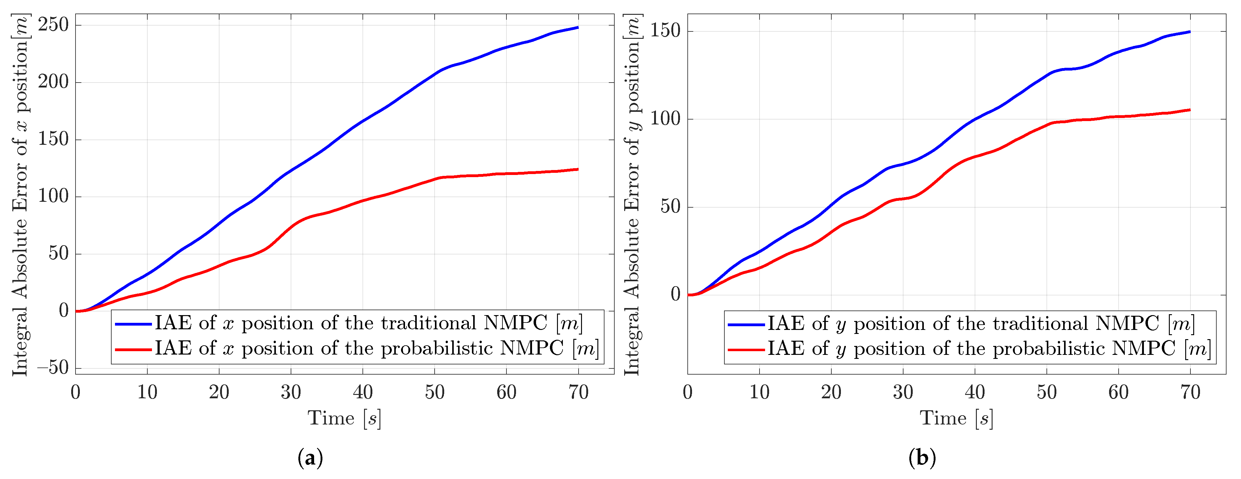
Since both traditional and probabilistic NMPC control simulations have Gaussian noise acting on them, there is always some tracking error; however, the probabilistic NMPC eliminates the mean value of the disturbance because of the observer. In contrast, with the traditional NMPC, the system fails to reach the target position, leading to excessive cumulative error, as also shown in Figure 7.

So, the probabilistic NMPC controls the system with smaller integral absolute errors (IAEs) than the traditional NMPC. For x, in 70 s, the probabilistic NMPC creates a 124.115 m IAE, but the traditional NMPC creates a 248.284 m IAE, so the traditional NMPC has approximately 100% m more IAE. For y, in 70 s, the probabilistic NMPC creates a 105.418 m IAE, but the traditional NMPC creates a 149.93 m IAE, so the traditional NMPC has approximately 42.22% m more IAE.

Furthermore, Figure 8 and Figure 9 show the control input and the observed control input disturbances of the probabilistic NMPC for the corresponding input signals $F_1$, $F_2$, $F_3$, and $F_4$. When the probabilistic NMPC-controlled vehicle tracks the reference of the ramp function up to the target point, the vehicle thrusters do not exceed the limits of the input constraints. However, when the vehicle encounters the obstacles, especially the stationary obstacle, the control inputs go to bigger values, and unlike the traditional NMPC, which has no constraints, the probabilistic NMPC operates the vehicle within the calculated constraints. One can see that the output of all disturbance observers follows the mean of the input disturbance, which is −7.5 N.

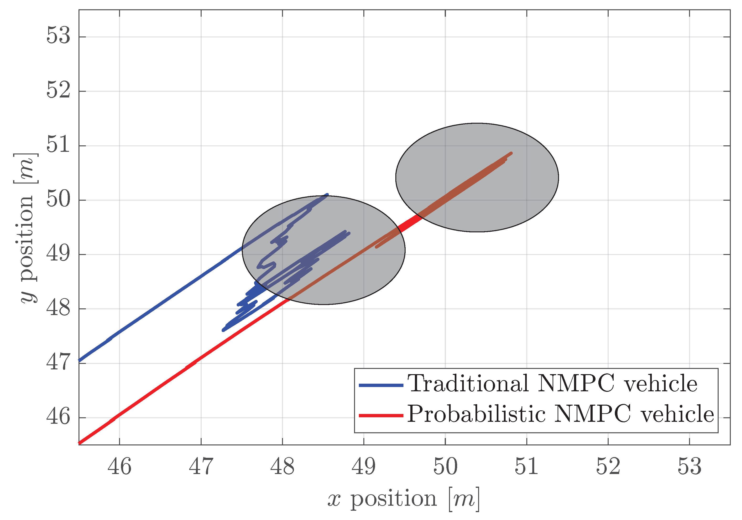
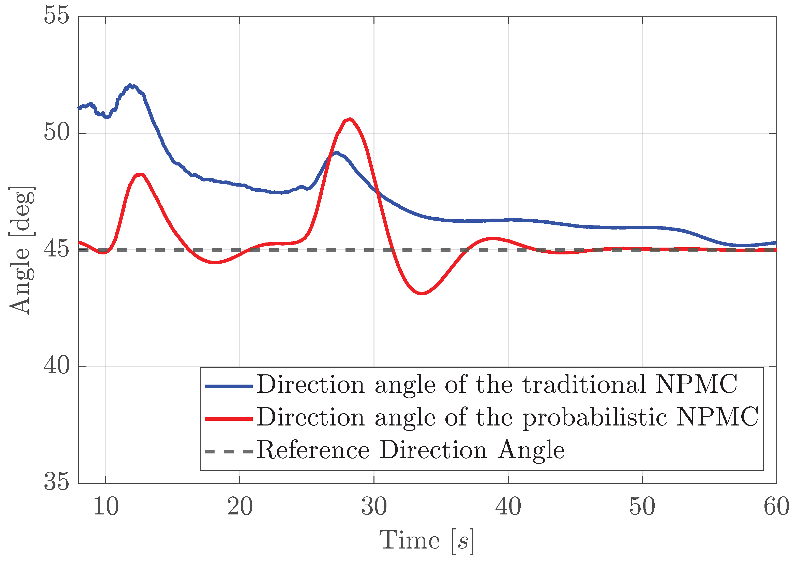
Finally, Figure 10 shows the close-up look of both traditional and probabilistic NMPC controllers when they reach the target point. As we can visually see, the probabilistic NMPC creates a more subtle trajectory than the traditional one. In addition, Figure 11 shows the direction angles of both traditional and probabilistic NMPC when they are avoiding obstacles and reaching the target point. One can see that the probabilistic NMPC tracks the 45° angle quite reasonably while avoiding the obstacles approximately at 11 and 26 s, but the traditional one struggles due to the water current.

8. Discussion and Future Work

The proposed method achieves better tracking performance under non-zero-mean probabilistic constraints with less steady-state error, simultaneously avoiding stationary and moving obstacles compared to the traditional NMPC. However, while Cantelli’s inequality provides a framework for probabilistic constraints, it can be conservative; therefore, it would be beneficial to investigate less conservative methods to address the probabilistic constraints.

The magnitude of the disturbances that can be attenuated is limited by the actuator reaction and working torque range. In addition, the actuators are assumed to be providing an ideal control signal. However, in real applications, actuators also have their own dynamics that can affect our performance due to their limitations.

In addition, in this study, it is assumed that the positions and velocities of the obstacles are known. The uncertainties in the positions and velocities of obstacles and dynamic obstacles are not considered. If the vehicle has the equipment to measure the positions and velocities of dynamical obstacles, the proposed method is still applicable by updating the velocity obstacle cones at each sampling instance with the updated measurements. Otherwise, the considered velocity obstacle method cannot be applied in the existence of dynamic obstacles since the cones are established based on the velocities of obstacles.

Additionally, it is important to note that this work focuses solely on controlling a single-ego vehicle. However, in certain operations, it may be necessary to manage a group of autonomous vehicles to achieve consensus, and therefore, this should be considered in future work. In future work, we can also explore scenarios that involve uncertain or time-varying vehicle parameters.

For real implementation, an industrial PC equipped with a GPU can be considered, where the industrial PC has an interface with sensors and actuators, and the GPU can handle the heavy computational load of NMPC. Note that ship control systems are comparably slow, allowing the controller to be implemented with larger sampling periods, so even without GPU, high-computational-power industrial PCs can solve the proposed NMPC optimization in these sampling periods.

9. Conclusions

In this paper, we propose an extension of probabilistic linear MPC for nonlinear systems, enabling efficient operation across all operating points and under the effect of non-zero-mean disturbances. This extension is particularly tailored for uncrewed surface vehicles, incorporating probabilistic disturbance attenuation and stationary and moving obstacle avoidance. We highlighted the challenges of applying probabilistic linear MPC to nonlinear systems, where probabilistic signals in states and outputs change their mean and variance across different operating points. To address this, we utilized an EKF to estimate the mean value of the states at all operating points and a linear matrix difference equation to calculate the covariance matrix at each sampling instance via successive linearization. This method allows for the cost function and probabilistic constraints to be updated dynamically at each sampling instance.

We addressed non-zero-mean disturbances by separating them into deterministic and probabilistic components. The deterministic part, represented by the mean of the disturbance, was handled using a deterministic disturbance observer. Furthermore, the remaining zero-mean probabilistic component was integrated into the probabilistic MPC framework.

The simulation results showed that the proposed probabilistic NMPC allows the system to follow the reference path more accurately than traditional NMPC, eliminating steady-state errors relatively. In contrast, traditional NMPC exhibits significant steady-state errors and is unable to reach the target reference, as indicated by the absolute error and the integral absolute error results.