Article

Reliable Detection of Unsafe Scenarios in Industrial Lines Using Deep Contrastive Learning with Bayesian Modeling

by
Jesús Fernández-Iglesias
1,2,3,*,
Fernando Buitrago
2,4 and
Benjamín Sahelices
1,2,5
1
GIR GCME, Departamento de Informática, Universidad de Valladolid, Plaza del Colegio de Santa Cruz 8, 47002 Valladolid, Spain
2
Laboratory for Disruptive Interdisciplinary Science (LaDIS), Universidad de Valladolid, Plaza del Colegio de Santa Cruz 8, 47002 Valladolid, Spain
3
AI Department, WIP by Lear, C/ Cronos, 18, 47195 Valladolid, Spain
4
Departamento de Física Teórica, Atómica y Óptica, Universidad de Valladolid, Plaza del Colegio de Santa Cruz 8, 47002 Valladolid, Spain
5
Departament of Informatics, Universidad de Valladolid, Plaza del Colegio de Santa Cruz 8, 47002 Valladolid, Spain
*
Author to whom correspondence should be addressed.
Automation 2025, 6(4), 84; https://doi.org/10.3390/automation6040084 (registering DOI)
Submission received: 27 September 2025 / Revised: 16 November 2025 / Accepted: 25 November 2025 / Published: 2 December 2025
(This article belongs to the Section Industrial Automation and Process Control)

Abstract

Current functional safety mechanisms mainly control the access points and perimeters of manufacturing cells without guaranteeing the integrity of their internal components or the absence of unauthorized humans or objects. In this work, we present a novel deep learning (DL)-based safety system that enhances the safety circuit designed according to functional safety principles, detecting, with great reliability, the presence of persons within the cell and, with high precision, anomalous elements of any kind. Our approach follows a two-stage DL methodology that combines contrastive learning with Bayesian clustering. First, a supervised contrastive scheme learns the characteristics of safe scenarios and distinguishes them from unsafe ones caused by workers remaining inside the cell. Next, a Bayesian mixture models the latent space of safe scenarios, quantifying deviations and enabling the detection of previously unseen anomalous objects without any specific fine-tuning. To further improve robustness, we introduce an ensemble-based hybrid latent-space methodology that maximizes performance regardless of the underlying encoders’ characteristics. The experiments are conducted on a real dataset captured in a belt-picking cell in production. The proposed system achieves 100% accuracy in distinguishing safe scenarios from those with the presence of workers, even in partially occluded cases, and an average area-under-the-curve of 0.9984 across seven types of anomalous objects commonly found in manufacturing environments. Finally, for interpretability analysis, we design a patch-based feature-ablation framework that demonstrates the model’s reliability under uncertainty and the absence of learning biases. The proposed technique enables the deployment of an innovative high-performance safety system that, to our knowledge, does not exist in the industry.

1. Introduction

Automated manufacturing environments have almost completely replaced manual assembly lines in all areas of the industrial ecosystem, from machinery and vehicle manufacturing to the chemical and energy sectors. This transition extends to other sectors, including food, textiles, and various other manufacturing industries. For this reason, productivity has increased drastically, thus improving the added value of these sectors and generating wealth and progress. However, the number of accidents involving damage to human life and/or economic losses in the industrial sector is among the highest in all the sectors of economic activity (see [1,2] for data from the industrial sector in the United States and the European Union). The potential social and economic impact of these unsafe conditions is very high. For example, in 2024, the industrial sector in the European Union represented a 19% share of the total gross value added [3], whereas in the United States the manufacturing industry represented 10% of the total gross domestic product [4]. These data can easily be extrapolated to the world economy if it is taken into account that the United States and the European Union represent 26% and 14% of the world economy, respectively.
A significant percentage of accidents occur within automated manufacturing lines. Ref. [5] presents a study analyzing 369 accidents involving robots that caused injuries to operators in Korea during the 2010–2020 period, showing that more than 95% of the robot-related accidents occurred in manufacturing businesses, while the remaining 5% were reported from the service and construction sectors. These manufacturing lines are characterized by complex high-energy interactions of different heavy industrial elements. Therefore, the consequences of accidents are potentially serious from the perspectives of both humans and materials. Currently, all new machines operating in European territory must comply with functional safety standards that guarantee the safe and correct operation of their components, so it is required to comply with the essential health and safety requirements (EHSRs) of Machinery Directive 2006/42/EC. To that end, safety is designed according to a series of standards harmonized with the previous directive, mainly ISO 13849-1 [6] (safety of mechanical, hydraulic, and pneumatic products) and IEC 62061 [7] (safety of electrical, electronic, or programmable electronic systems and products). An equivalent regulatory framework exists in the United States, where machinery safety is governed by Occupational Safety and Health Administration (OSHA) regulations (29 CFR 1910) and the American National Standards Institute (ANSI) B11 series of standards, defining the requirements for machine safeguarding and risk reduction. However, in many cases, these measures have limited effectiveness as they can easily be overridden or avoided by operators with insufficient training and subject to careless operation. The most relevant consequence is that an operator can remain inside the safety perimeter of the assembly line when the production cycle starts. This invasion, whether partial or total, involves the creation of an illegitimate (unsafe) scenario with potentially fatal consequences for people. There is another group of consequences derived from the possible reconfiguration of the scenario by changing the position of some components or including new objects. These are also illegitimate scenarios that may affect the reliability and integrity of the industrial process, with potentially significant economic consequences.
Every illegitimate scenario should be identified in a robust way, although the current safety measures do not cover this. To overcome this, we propose designing a deep learning (DL)-based parallel safety system that is capable of detecting the aforementioned situations and enhancing traditional safety measures already existing in the manufacturing cells. The logical interaction between traditional safety devices (e.g., doors, light curtains, and emergency stops) and the proposed system can be seen in Figure 1. When the safety signal is broken in any of the classic devices, the machine will enter into a safe state. Additionally, when the safety circuit is closed, the AI system can interrupt it when detecting illegitimate scenarios that have bypassed standard safety measures. The proposed system is consistent with ISO 12100:2010, which defines the general principles for machinery design, risk assessment, and risk reduction. This standard specifies that complementary protective measures involving additional equipment may have to be implemented when there is still remaining risk for persons. In this context, the proposed artificial intelligence (AI)-based parallel monitoring system can be regarded as an additional protective measure: it operates independently of the certified functional safety chain and provides early detection of illegitimate scenarios, such as human presence or foreign objects inside manufacturing cells.
In this work, we have developed a supervised DL methodology based on contrastive learning (CL) that is capable of synthesizing the information that characterizes the normal operation state of an industrial facility and discriminating, with absolute certainty, the presence of workers within it. Additionally, by modeling the latent-space distribution of the safe scenarios by means of Bayesian clustering, and without performing any additional fine-tuning, the system is capable of detecting potentially unsafe scenarios caused by the presence of anomalous objects that were not seen during the learning process. In order to assess the model’s performance in uncertain situations and provide explainability for its decisions, a patch-based input-feature-ablation method is proposed. The interpretability analysis reveals the absence of bias and the use of relevant information in the decision-making process. Both the industrial line used in the experimentation and all the data come from real sources (a production environment currently operational in a factory), increasing the reliability and robustness of our proposal. All of the above constitutes a framework that demonstrates the reliability and robustness of our proposal to ensure detection of unsafe situations. In addition, the presented methodology can be deployed in any industrial cell, complementing the safety measures specified by the functional safety standards. The rest of the paper is organized as follows. Section 2 reviews the main lines of research on the application of AI in architecture, engineering, and construction (AEC) environments, with an emphasis on risk detection and safety-related works. Section 3 describes the industrial configuration, the dataset used, the models, and the characteristics of the training carried out. Section 4 describes the experimental results. Section 5 describes the Bayesian analysis for the identification of unknown non-legitimate scenarios. Section 6 presents the designed patch-based input-feature-ablation method and covers the explainability analysis. Section 7 details the industrial configuration that has resulted in the integration of the AI safety channel into a real manufacturing cell and presents the main limitations encountered in the study, as well as future lines of work. Finally, Section 8 describes the conclusions of our work.

2. Related Work

Our work is related to the existing literature on quality control and risk detection in AEC environments, industrial anomaly detection, and the integration of AI systems with functional safety methodologies. The quality and safety of AEC working environments can be addressed from many different perspectives. For example, there is a large number of studies focused on the control of manufactured products (see [8,9,10] for practical applications). Other recent works refer to the detection of the use of appropriate equipment by operators [11,12,13,14,15,16,17]. Another relevant line of research is the detection of safety risks by analyzing scenarios using DL technology and generating a risk classification to prevent accidents [18,19,20,21,22,23]. Worker ergonomics automatic analysis also takes up a significant portion of scientific production in this area [24,25,26]. This and other works (see [27]) focus on the study of specific individual characteristics that represent a small part of complete AEC-related processes and environments. In this work, we developed a methodology that checks the safety and suitability of an industrial manufacturing process by monitoring the entire process rather than looking at specific characteristics of it. This allows us to detect, for example, whether the trajectories and movements of a welding robot are as expected (rather than checking the final weld or the presence of components) or whether there are workers in forbidden production areas rather than simply observing whether they are wearing the appropriate personal equipment. Ref. [28] proposes the use of a YOLO V8-based scheme to monitor in real time a stamping press process, detect potential dangers, and reduce the number of accidents. Our study, although framed in a similar context, is more ambitious since it also detects potentially dangerous anomalous situations caused by any kind of object commonly found in manufacturing environments, like tools, cleaning utensils, wires, or components misplaced from another industrial process. Since the set of objects is virtually unlimited, it cannot be learned using a traditional supervised learning mechanism, as presented in [28], and some anomaly detection capabilities are required.
Anomaly detection is a major research niche of considerable industrial relevance. One prominent domain where it has been extensively applied is predictive maintenance. Ref. [29] presents a hybrid anomaly detection model based on DL that predicts downtime within the manufacturing process by analyzing raw equipment data. Ref. [30] proposes a deep echo state network (DeepESN)-based method for predicting the occurrence of machine failure by analyzing energy consumption datasets from production lines. Anomaly detection can also be useful for checking manufactured products’ quality. Ref. [31] introduces ReConPatch, a CL-based framework that extracts easily separable features by training a simple linear transformation, demonstrating its performance in widely used industrial quality control datasets (MVTec AD and BTAD). Using the same datasets, Ref. [32] proposes a CL scheme based on two stages. First, a discriminator learns to locate anomalies in the input images, and then this discriminator is used to train a CL scheme by providing negative-guided information. Our work does not study in detail the occurrence of anomalies in signals emitted by specific machinery (predictive maintenance) or attempt to quantify deviations in the quality of manufactured products. Rather, it focuses on detecting visual anomalous situations that may affect the entire industrial manufacturing process and the interaction between different pieces of equipment in an industrial facility. Other works that have some relation with ours include [33,34]. While the former one reviews the potential impact of applying a wide range of DL techniques to study anomaly detection within industrial control system (ICS) environments, the latter proposes a CL scheme with data augmentation through negative sampling for anomaly detection in actual operating systems in corporate environments. Similar to ours, these studies focus on detecting anomalies in complex systems characterized by the interaction of different processes. However, our work focuses on the use of 2D information captured with industrial cameras, while the other studies focus on the use of one-dimensional signals and data matrices without visual information.
Understanding how an AI model will behave in an unexpected situation remains a challenge today and is an active area of research. As a result, applying functional safety certification frameworks to AI-based products remains challenging. Ref. [35] reviews why the general DL-based system development process clashes head-on with the traditional safety development pipeline and proposes an integration architecture between DL systems and traditional safety devices that extends widely adopted functional safety management (FSM) methodologies. This perspective enables the integration of AI techniques, such as those developed in this work, as complementary channels that enhance the capabilities offered by traditional functional safety designs. Furthermore, as detailed in [36], an RSS must have characteristics such as modularity, integrability, and comprehensibility, among others. The AI system proposed in this study fulfills these characteristics. In terms of modularity, the new safety channel offered by the AI operates independently from the functional safety ones, complementing them without affecting their operation. In terms of integrability, the AI-managed channel can be incorporated into a safety system designed using functional safety standards as described in [8] (details about the deployment can be seen in Section 7). Finally, regarding comprehensibility, the proposed AI system offers interpretability measures that enhance transparency and clarity in the inference process performed by the AI (see Section 6), improving the understanding, safe-state recovery, and maintenance of the system.

3. Methods

3.1. Industrial Configuration

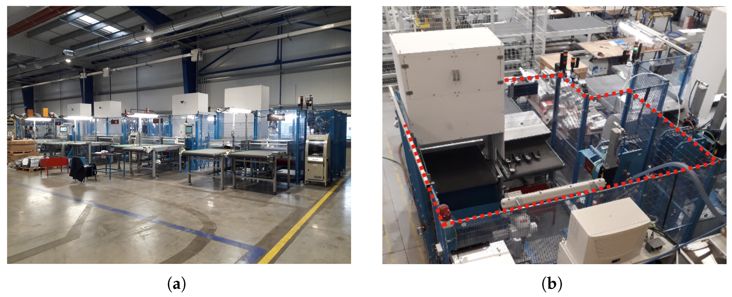
The physical environment from which we obtain the data used in this work can be seen in Figure 2. It is composed of several manufacturing cells, located in parallel, which perform a press welding process (Figure 2a). The parts to be welded are picked up and placed on two different conveyor belts. Physical fences and safety doors are the only functional safety elements that protect each of the cells (blue fences in Figure 2b). However, this safety standard does not guarantee that foreign objects cannot remain inside the closed perimeter at the moment of starting the production cycle, which may cause serious damage to humans and/or equipment.
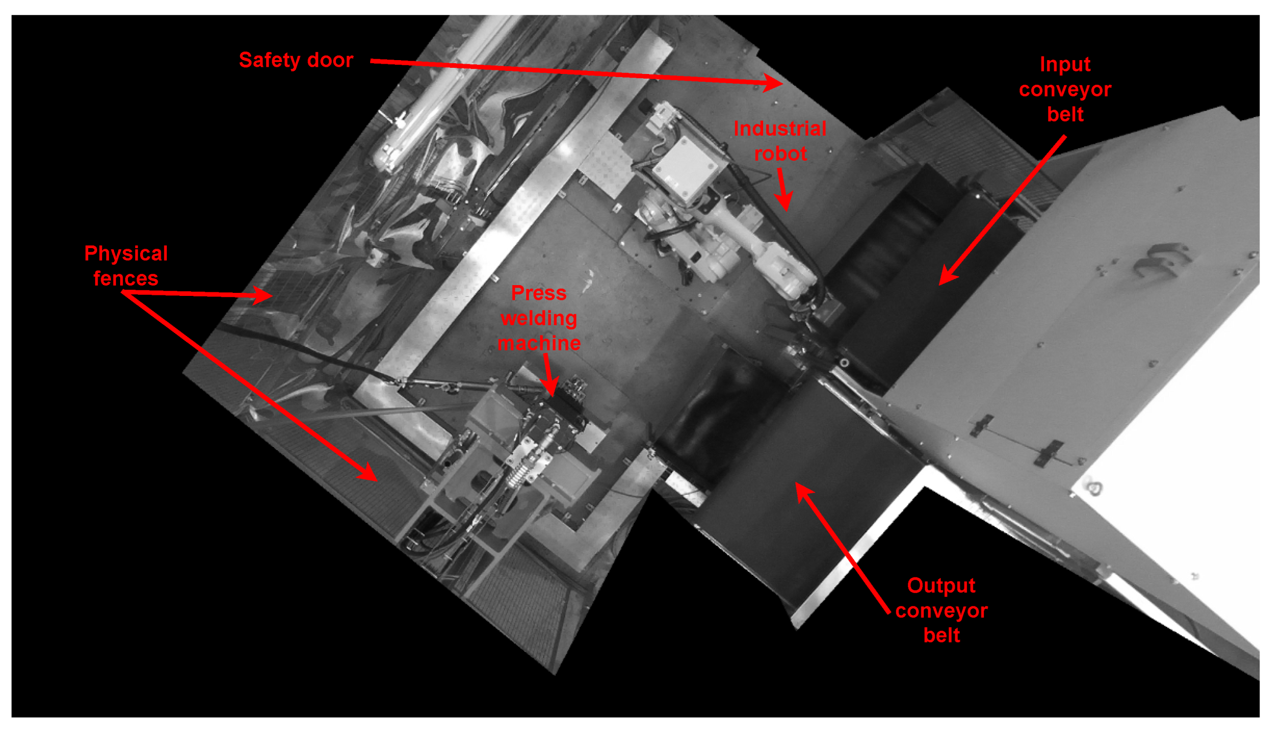
A data capture infrastructure is placed in each individual cell. We use an RGB-D stereo camera with a resolution of 2 megapixels (1920 × 1080) delivered at 30 frames per second. To cover the entire working area, the camera is placed in a top-down position. Thus, each pixel covers approximately a 4 × 4 mm region of the cell’s inner surface. Depth information is discarded since it is very noisy, which would hinder an accurate and robust analysis. Additionally, RGB images are converted to grayscale to emphasize the structural characteristics of the image and to increase robustness against illumination changes. Since the images provided by the camera cover more area than required, a binary mask is constructed to indicate the region to be inspected, so the noise from outside the cell is filtered out and its potential bad influence. An example of the inspection area captured by the camera, after applying the masking, can be seen in Figure 3. This simple data acquisition method can be easily adapted to different topologies and types of cells, ensuring simple and robust scalability.

3.2. Dataset

When building the dataset representing the safe operation of the facility, it is important to guarantee that the manufacturing cell always remains in legitimate scenarios (safe states). These scenarios are very diverse because the cell has multiple mobile elements that interact in complex ways, leading to a wide range of possible configurations. For example, there may be one or more robotic arms, conveyor belts, welding presses, and wires, among other objects that may move. The appearance of volatile elements, such as smoke, sparks, and small flames, is also possible, all within the normality of the manufacturing cell. Thus, it becomes crucial to build a diverse and representative dataset of the normal activity of the manufacturing cell. To this end, the production process is sampled during a significant number of cycles, ensuring coverage of all workflows and scenarios that do not endanger the safety of the process.
In addition to correct scenarios, it is necessary to capture situations that may compromise the safety of the industrial process. Two groups of incorrect scenarios are identified depending on whether people are involved or not. The most hazardous element that can be found inside the manufacturing cell is a person because the possible consequences are serious damage, disability, or even death. Thus, it is essential for the system to robustly detect situations in which people, partially or totally, are inside the production perimeter. Consequently, we feed the dataset with images of people within the monitored area. These images are captured during the assembly of the installation (mechanics), programming of the robot trajectories (programmers), and other situations that occur during the machine setup, ensuring that the cell assembly fine-tuning process is not interrupted. Additionally, under strict safety conditions, complex situations have also been forced, with humans partially covered by machinery, to test the detection capabilities of the developed methodology. All individuals from whom images were captured to support the experimentation presented in this work have been comprehensively informed and have provided their consent.
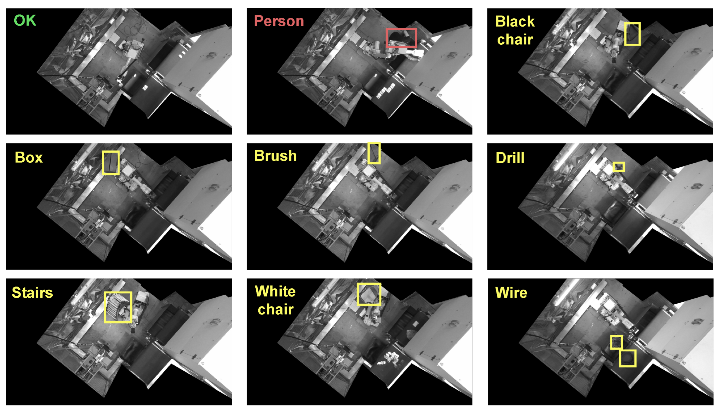
The second group of incorrect scenarios relates only to the appearance of new strange objects. This second group could potentially have infinite variability because it is not possible to restrict the number or type of objects that can appear in the scenario. It is therefore not possible to train our models for all possible situations. Nevertheless, the objective of this work is to detect any kind of uncertain scenario caused by the presence of any strange object. To achieve this, we have developed a novel proposal based on latent-space Bayesian analysis described in Section 5. With the sole purpose of testing our proposals (not to train with them), a dataset of scenes with the presence of different types of strange objects has been generated. All collected objects are commonly found in industrial manufacturing environments and used during machine maintenance and repair, so it is easy for them to remain inside the cell in case of human negligence. A summary of the collected dataset can be found in Table 1. Figure 4 shows an example of an observation from each category. It can be easily seen how strange objects can appear in any area of the cell surface, making it hard for a human operator to check the safety of the cell. Furthermore, some of these objects can be quite small (brushes, drills, and wires) and may be partially hidden by some elements of the cell, making their detection extremely challenging.
In order to increase the variability of our dataset, we deliberately included different lightning conditions. The first was the different ambient light in the industrial plant. To this end, images were captured over a period of 12 consecutive days at different hours. Second, images of the installation were captured by varying the power of the different LED lighting devices integrated in it. In this way, a balanced dataset is constructed, containing a wide range of realistic lighting conditions that, if not considered, can impact the performance of the models.
An essential step when building a real-world dataset is to check for the presence of biases that may distort the final results. This event typically leads to unexpected behaviors when the system is in production. In the context of this problem, a biased dataset would be, for example, one in which the situations that may compromise the safety of the cell have been captured when the industrial machinery is in unrealistic positions. This would cause the industrial configurations present in the safe and unsafe scenarios to be so different that the DL models could associate the anomalous situations with certain positions of the machinery rather than basing their decision on the strange object. Another biased situation would be one in which unsafe elements were always located in a similar position. This would not allow extrapolating the performance of the models to the entire surface of the cell. To address this problem, we have conducted two different studies: distribution of embeddings and location of unsafe elements in the cell layout.
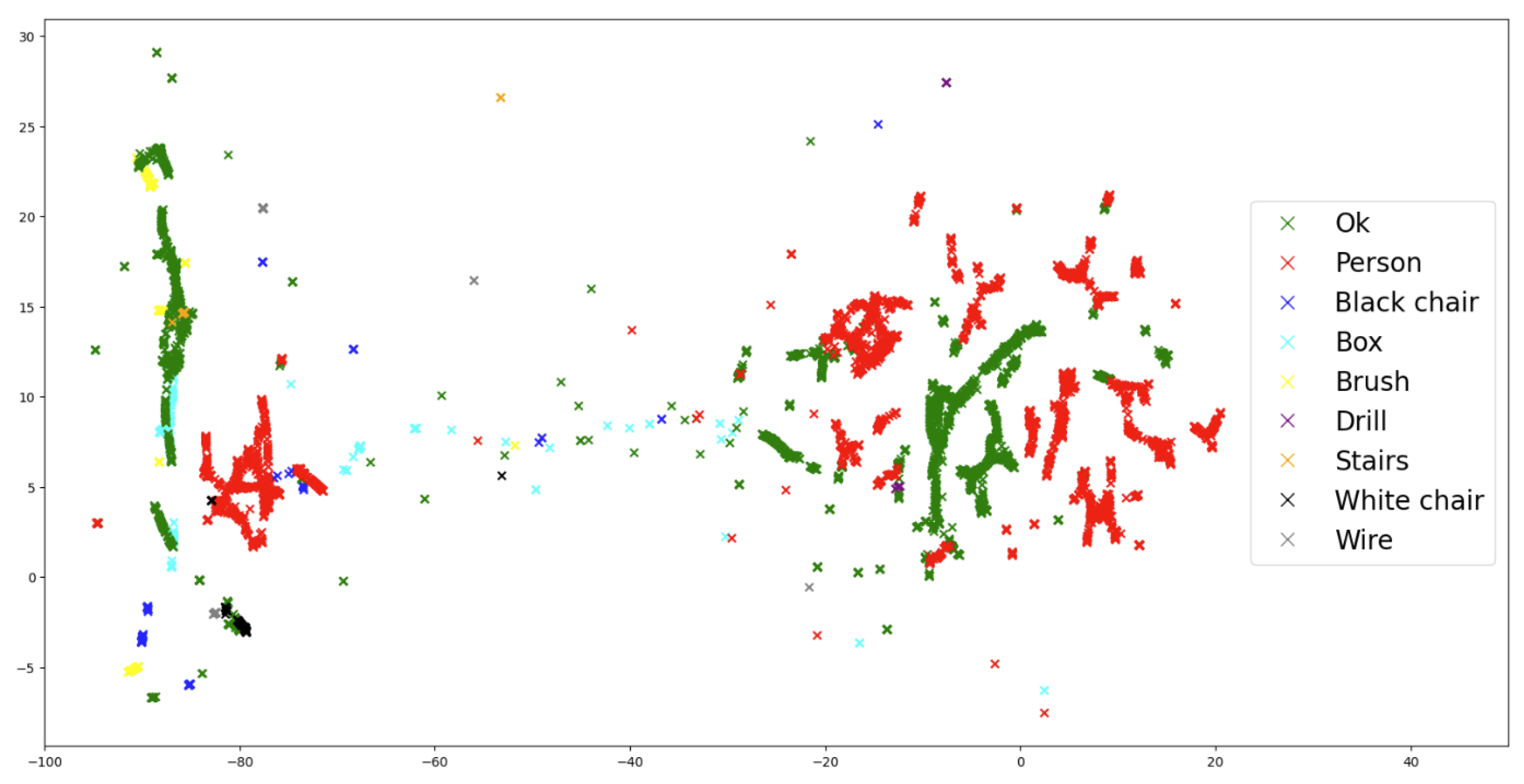
For the first one, we use the pairwise controlled manifold approximation projection (PaCMAP) technique. This methodology, presented in [37], is more suitable for obtaining low-dimensional representations of high-dimensional datasets than other widely used dimensionality reduction techniques, such as UMAP or t-SNE. The main reason is that it is capable of obtaining a latent representation that preserves both the local and global structure found in the original dimensional space, while other techniques do not. We choose the standard parameter configuration: 10 neighbors for the k-nearest neighbor graph, 0.5 as the ratio of the number of mid-near pairs to the number of neighbors, 2 as the ratio of the number of further pairs to the number of neighbors, and principal component analysis (PCA) as the initialization of the lower-dimensional embedding. The obtained R 2 embedding representation can be seen in Figure 5. First, it can be seen how the representations of Ok and person images are mostly intertwined and distributed evenly throughout the latent space without forming obvious clusters that would make them easy to isolate. This is essential as both categories are responsible for guiding the supervised learning process described in Section 3.3. The anomalies are also spread across different regions of the space. When the foreign object is very small (such as the drill), the associated representations are completely camouflaged in areas with a predominance of safe images. It is also noteworthy that, when the object is larger and has greater contrast (black chair or brush), sometimes clusters are formed with a predominance of that object given that it differs greatly from other situations present in the dataset However, when the same object is in other positions, it seems to blend in more with situations already collected in the rest of the categories. Overall, the obtained latent space does not seem to reveal the presence of clear biases or situations indicating a skewed dataset.
For the second study, we have created Figure 6, which shows, by category, the location of the different unsafe or potentially unsafe elements. To achieve this, the middle point of the objects has been manually labeled in all potentially unsafe images and in a random subset of 850 unsafe images (persons). To enhance visualization, contour curves have been plotted, encompassing the most densely populated regions from the 50th percentile to the 99th percentile. It can be appreciated that, on average, the different categories are distributed uniformly throughout the different spaces of the cell. There is no category that is only found at a very specific point in the installation, thus demonstrating the balance between categories and the variability of the dataset.

3.3. Supervised Deep Contrastive Learning

The number of scenarios that can lead to an unsafe state of the cell is practically unlimited. This precludes the use of standard supervised learning models to search for anomalous situations because these kinds of algorithms require a predefined number of classes, i.e., infinite in this case. One possible approach involves the use of unsupervised learning, namely autoencoder-based schemes (see [38]). These schemes map each correct scenario to a distribution in the latent space. An inaccurate reconstruction of a sample from the learned distribution could indicate the presence of a strange setup that may compromise the safety of the cell. However, this approach suffers from two main drawbacks. First, such schemes tend to over-smooth the reconstructions due to the use of Kullback–Leibler divergence in the loss function (see [39]). As a result, the great complexity and variance inherent in the correct scenarios could potentially lead to a problem of persistent false positives (scenarios incorrectly categorized as unsafe), triggering false alarms and thus impacting the productivity of the industrial process. Second, these kinds of solutions are not able to discriminate, and therefore prioritize, between different objects. For example, a person’s foot may occupy the same surface as a drill but comprise very different scenarios; the former situation involves far greater risk than the latter. It is essential to ensure that the most dangerous scenarios (people inside the cell) will be detected over any other situation.
In order to overcome the aforementioned challenges and endow the system with the appropriate safety capabilities, we propose the use of deep CL. CL is an emerging technique that aims to extract meaningful representations of the input features by contrasting positive and negative pairs of instances. It leverages the assumption that similar cases should be close to each other in a learned latent space, while dissimilar cases should be farther apart. In a standard CL approach, a single positive of each anchor (a slight augmentation of an observation) is contrasted against any other image in the dataset. Thus, the need for supervised learning (labels) is avoided, and a topology of representations is generated in the latent space based on the similarities of the extracted features. The problem is that this self-supervised approach would not guarantee that safe and unsafe scenarios lie in regions far enough from each other because sometimes their discrepancies are minimal. This is a very important problem in our context because we have a set of highly diverse scenarios that belong to the same positive class (safe scenario), and the same applies to the negative class. In addition, we have two subsets in the negative class: the intrusions of people, very relevant, and the presence of any foreign object. Therefore, the objective is to project all the images of the positive class in a narrow region of the latent space and, at the same time, keep this region as far away as possible from the representations of the scenarios that seriously compromise the safety of the cell. For this purpose, our learning scheme relies on the supervised version of the CL paradigm of [40], which meets our requirements.
The supervised CL scheme will be trained with only two categories of images: Ok (representing the safe state) and Ko (representing humans within the industrial perimeter). This approach has two main advantages. First, by using supervised training with humans, it is guaranteed that the system will deliver excellent performance to avoid situations that may compromise people’s integrity. Second, models are trained to synthesize the complex set of features that characterize a correct scenario, learning that any perturbation of these features must be projected into a distant region of latent space. This behavior implies that disturbances caused by a wide range of uncertain and potentially dangerous situations can be resolved without the need to train the network with all the specific cases, which would be impossible. Experimentation associated with the detection of the most dangerous scenarios is described in Section 4, while the uncertainty management for the detection of strange situations (any foreign object) is shown in Section 5.

3.4. Training Specifications

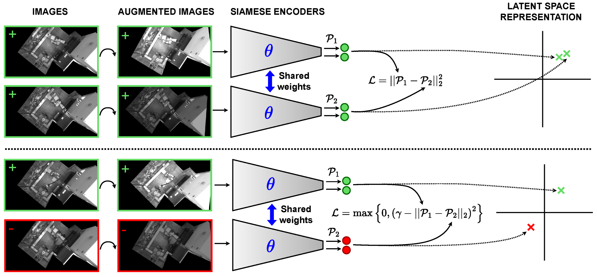
The designed architecture scheme can be seen in Figure 7. Our approach adapts the idea presented in Simple Framework for Contrastive Learning of Visual Representations (SimCLR; see [41]), which targets robust label-free representations of images by applying random data augmentation techniques. We adopt the same concept but using the supervised CL scheme explained in Section 3.3. We design random data augmentation transformations, aiming to achieve robustness against the different perturbations that a capture device may encounter in an industrial manufacturing production environment. Mainly, these disturbances arise from changes in ambient light conditions and vibrations of the capturing device. Therefore, the data augmentation transformations used are based on color space and geometric space alterations (see taxonomy in [42]). To this end, rotations, translations, brightness changes, and Gaussian noise are randomly applied at each epoch to the images that are introduced to the network. We compose all the aforementioned transformations, allowing the model to learn better representations of the data, as discussed in [41]. A visual effect of these augmentations can be appreciated in Figure 7. With this technique, we ensure consistent system performance when faced with variable physical conditions, which is very common in an industrial deployment. We note that this work does not intend to measure the effect caused by the inclusion of augmentations but rather chooses those most aligned with the alterations that images captured by a camera deployed in an industrial environment may encounter.
Regarding the models, we propose to implement a wide variety of configurations to demonstrate the effectiveness of our proposal regardless of the specific characteristics of each particular design. To this end, we use encoders from three widely used state-of-the-art convolutional neural network (CNN) families: ResNet ([43]), DenseNet ([44]), and EfficientNet ([45]). We also use a ConvNeXt network, a modern transformer-inspired CNN architecture that leverages the power of depth-wise convolution to deliver superior performance on vision tasks (see [46]). Finally, we also utilize a Cross-Covariance Image Transformer (XCiT; see [47]), a transformer architecture that combines the accuracy of conventional transformers with the scalability of convolutional architectures by leveraging a transposed version of the self-attention mechanism that operates across feature channels rather than tokens. From the ResNet family, we use the version with 18 hidden layers, from the DenseNet family the variants 161 and 201, and from the EfficientNet family the smallest model, B0. For ConvNeXt and XCiT architectures, we use the nano versions. The reason is that large transformer and transformer-inspired architectures typically require larger amounts of data to achieve comparable performance to CNNs (see [48,49]), and the dataset in this work is relatively small. For all models, we start the learning process from a pretrained version on the ImageNet dataset (see [50]). Thus, we achieve a faster convergence and reduce the computational cost as the models have already learned basic features useful for many types of computer vision problems regardless of the context and the specific task.
We propose to use the contrastive loss function in Equation (1), where x i , x j represent a pair of augmented images, y i , y j represent the corresponding labels, h θ i the i t h branch of the siamese neural network, and γ the margin that defines a threshold distance in the embedding space. In this work, we empirically set γ = 2 since it represents a sufficient margin to allow the CL process to clearly separate Ok and Ko observations in the latent space, but this hyperparameter may vary depending on the problem. For images of the same class (two positive examples; y i = y j ), the loss function tries to minimize their square Euclidean distance in the latent space. For images of different classes (positive and negative examples; y i y j ), it seeks to maximize their embedding square Euclidean distance at least as far as indicated by the γ margin.
L = | | h θ 1 x i h θ 2 x j | | 2 2 , if y i = y j . max 0 , γ | | h θ 1 x i h θ 2 x j | | 2 2 if y i y j .
In addition to data augmentation, we employ two further regularization techniques. First, we perform L2 or Ridge regularization in order to keep the weights of the model small, learn simpler representations, and therefore generalize better to unseen scenarios. Second, we select the best model achieved on the validation set over all training epochs (200), avoiding the effects of potential overfitting in the final stage of the learning process. We use the Adam optimizer [51] and an initial learning rate of 0.001, dynamically multiplying it by a factor of 10% if learning plateaus during ten consecutive epochs.
To validate our methodology, we divided the dataset into four subsets: train, validation, supplementary train, and test. While train and validation subsets are used to perform the learning process of the neural networks, the supplementary train and test subsets remain unseen at this stage of the process. Regarding the supplementary training subset, it is composed of a small subset of Ok situations, and it will be used to fit methodology after training DL schemes (more details will be provided in Section 4 and Section 5). With respect to the test set, it is composed of images not included in any previous subset, which will allow us to validate the overall process. It contains a subset of the Ok category, a subset of the Ko category (only humans), and all the scenes with objects that may potentially represent a risk to the cell’s safety (to preserve their uncertainty status). This last category, named Other objects, has not been used in the training phase. A summary of the number of elements contained in each dataset by category can be found in Table 2.
For the training process, we used a server with an NVIDIA RTX A5000 GPU with 24 GB RAM and an AMD Ryzen 9 5900X 12-core CPU. The training time is, on average, less than 5 h. This quick training time allows for a dynamic re-adaptation to a changing industrial environment that may require a slight fine-tuning of the system.
Figure 8 shows a schematic representation of the different phases of the proposed methodology. First, the camera is positioned in zenithal plane, adjusting the focus and shutter to maximize image quality. Next, the mask is defined to determine which areas will be inspected and which ones lie outside the cell. After collecting safe, unsafe, and potentially unsafe data, it is distributed into training, validation, supplementary train, and test datasets, with all anomalies going to the latter. Train and validation sets are used to train the CL model, while the third is used to adjust the Bayesian mixture. Finally, the algorithm is validated with the test set, and the solution is deployed in a real environment.

4. Experimental Results for the Base Safe/Unsafe Scenario

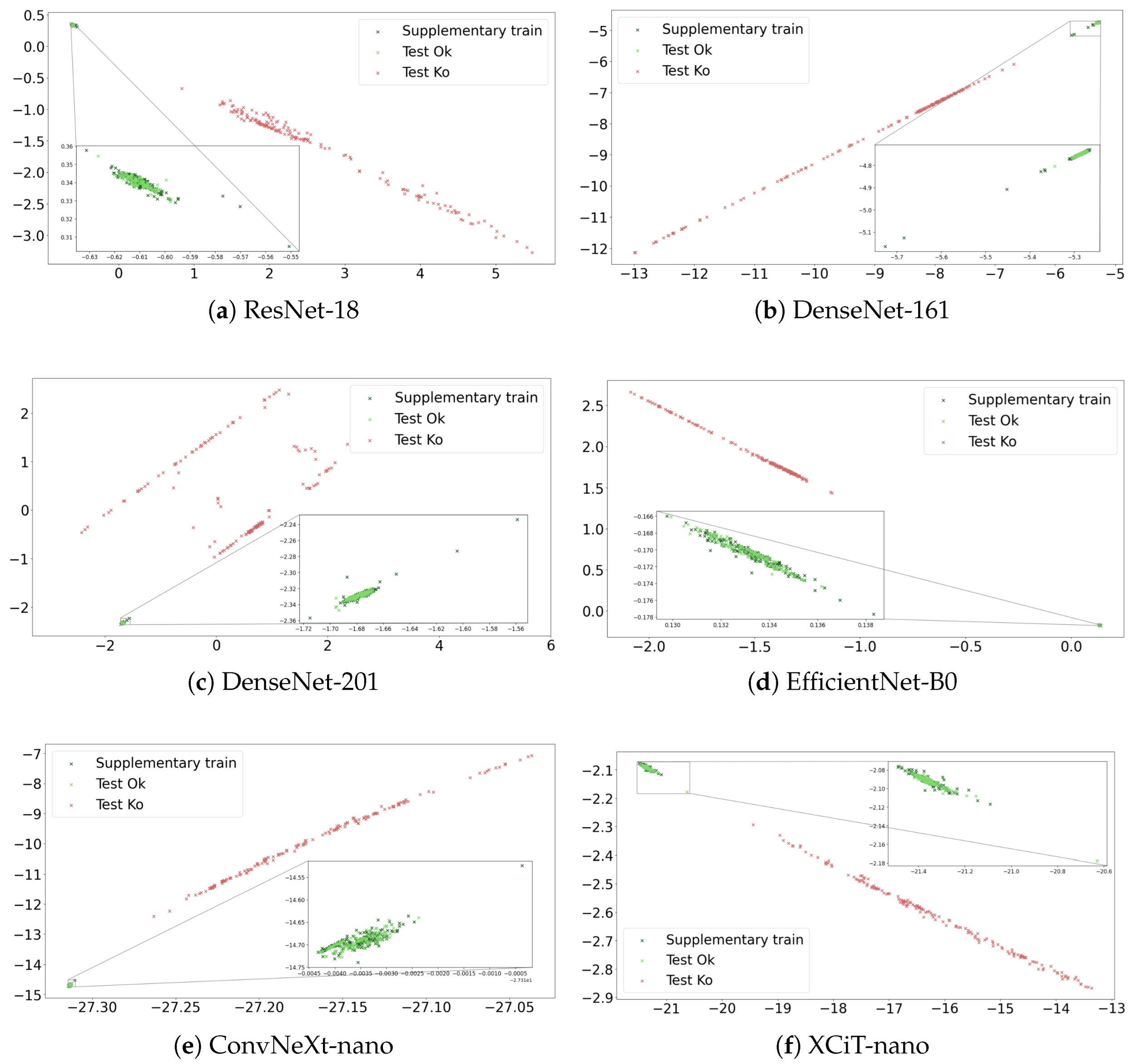
This section presents the results obtained for the problem of identifying the safe scenarios (Ok) from the most dangerous ones (presence of person; Ko). Figure 9 shows, for the supplementary train and test datasets, the distribution of the latent space learned by the six encoders detailed in Section 3.4. We note that, once the CL schemes are trained, the feedforward step can be performed through any of the two branches of the siamese networks to compute the latent-space representations. For all cases, we can identify two well-defined patterns. First, the Ok and Ko scenes from the test dataset are projected in regions far away from each other. This means that the CL schemes are correctly associating the disturbances produced by the presence of people as features that compromise the safety of the manufacturing cell. Second, it can be noticed that all the safe scenarios, either from the supplementary train or the test dataset (both not used in the training phase), form an isolated and compacted cluster. This means that the models are able to synthesize the underlying characteristics of the safe scenarios despite the great diversity among them.
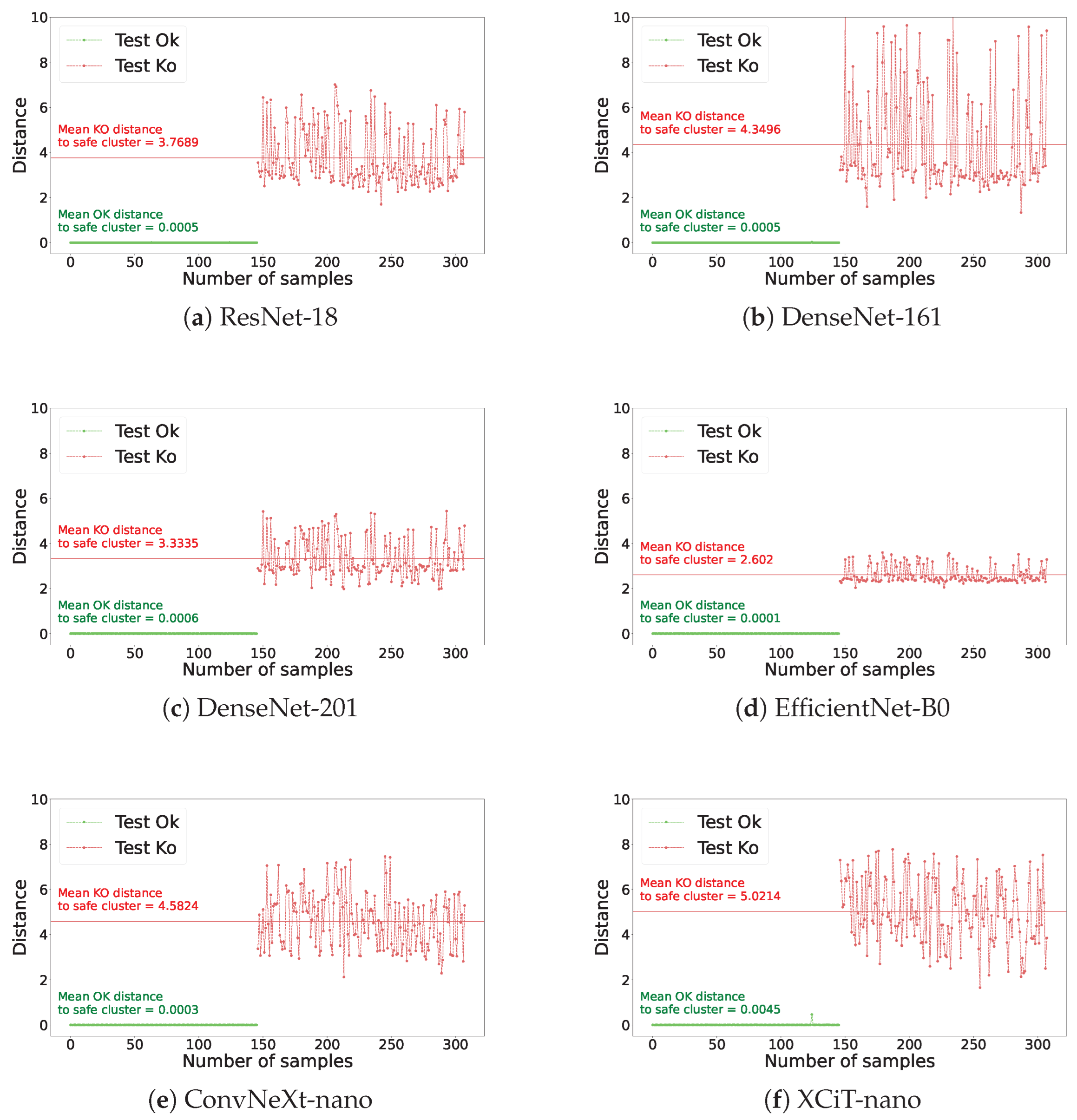
Beyond the latent-space morphology, it is necessary to define a strategy that assigns a new scenario to the safe or unsafe category. In this case, where the differences are clearly defined, a simple but useful technique is based on the nearest-neighbor search (see [52]). It is important to perform the nearest-neighbor fit using an auxiliary dataset not used in the training phase because, if the fit were conducted using the training or validation sets, the process would be biased by the model’s implicit knowledge of them and the results would not be representative. That is why we use the latent-space representations from the supplementary train dataset. Thus, we measure the Euclidean distance from each observation in the test dataset to its nearest neighbor from this supplementary dataset. The nearest-neighbor search is described in Equation (2), where ST and T represent the supplementary train and test datasets, h θ 1 one of the siamese network branches, and x t and x s t observations from the test and supplementary train datasets, respectively.
min x s t ST | | h θ 1 x t h θ 1 x s t | | 2 x t T
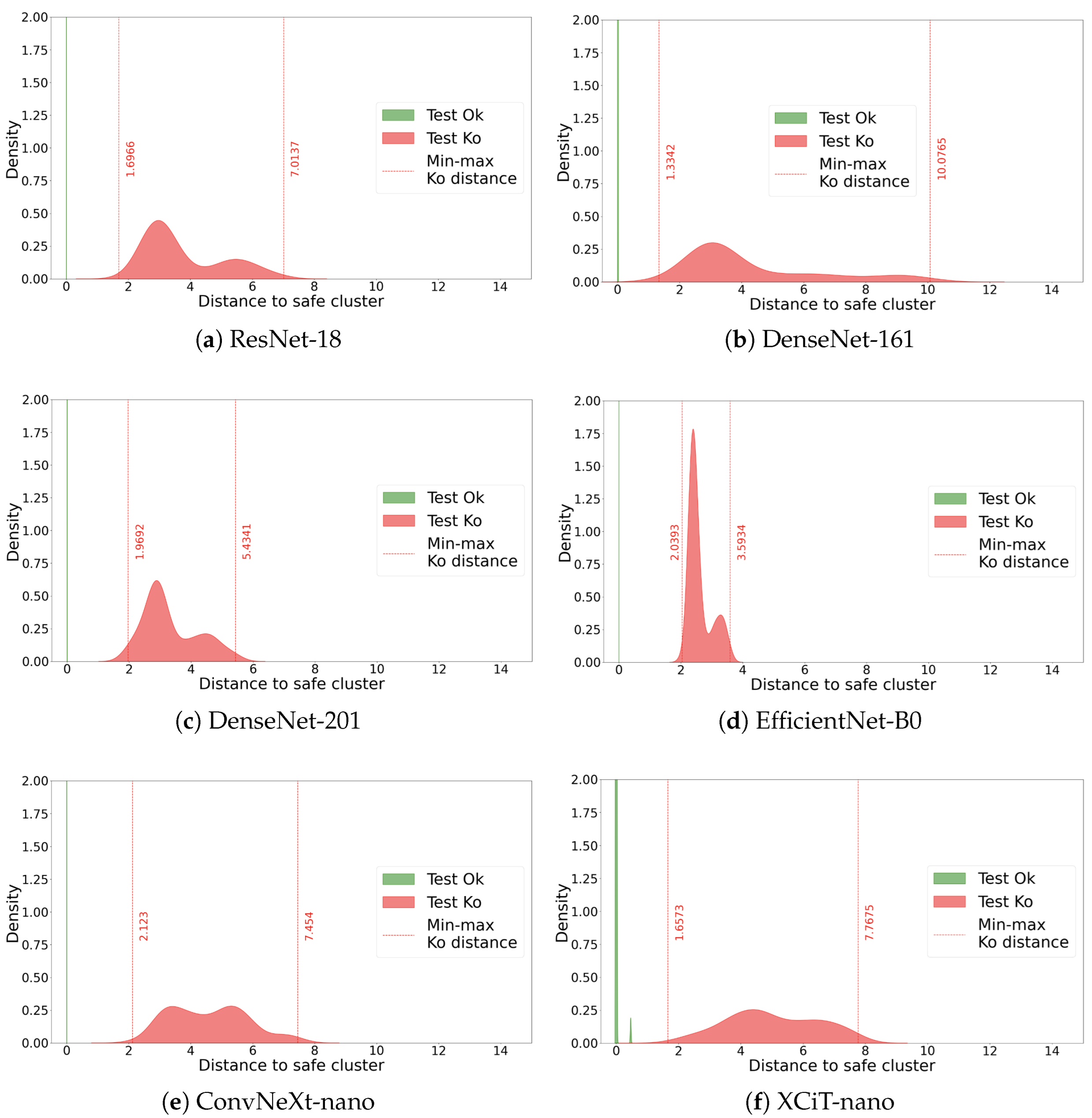
Thus, we quantify how distant each test set representation is from the nearest safe scenario. These distances are shown in Figure 10. It is easily noticeable how, for every network, all the distances obtained for the Ok class are notably smaller than all the distances obtained for the Ko class (remember that all instances in the supplementary dataset belong to the Ok class). For example, for the model ResNet-18, the average distance between a test set Ko instance and the safe cluster from the ST is 3.3335, whereas the average distance between an Ok instance and the same cluster is 0.0006. For all models, all Ko distances are about 3 to 4 orders of magnitude lower than the Ok ones. These results can be used to build a wide range of binary classifiers to diagnose whether a scenario is safe or unsafe. To this end, it is enough to set a threshold that lies at a midpoint between the distances of the Ok and Ko classes. The closer this threshold is to the average value of the Ok distances, the higher the probability that an unsafe scenario will not be misdetected. A second interesting aspect to discuss is the variance in the distances obtained for the Ko test set. For some models (DenseNet-161), it can be seen graphically that the variance is much greater than for other models (EfficientNet-B0). According to the loss function presented in Equation (1), the γ parameter defines the maximum distance at which it is necessary to separate Ok and Ko observations ( γ = 2 in this work). Thus, distances greater than γ will not result in a loss optimization and, therefore, in a better model fit. For this reason, even if the variance is higher for some models, as long as the distances are on average above γ , it is not significant in terms of the quality or performance of a model.
Lastly, instead of relying solely on a threshold to determine the degree of separation between the safe and unsafe clusters, a statistical analysis is carried out to demonstrate the effectiveness of contrastive learning schemes in isolating the distribution of Ok representations from the Ko ones. For this purpose, two statistics are calculated: the Mann–Whitney U test and the Pastore and Calcagnì overlapping index. While the former is used to test the null hypothesis that two samples come from the same population, the latter quantifies the similarity between two or more empirical distributions by using the overlap between their kernel density estimates (see [53]). Note that we conduct the non-parametric Mann–Whitney U test instead of a t-test because the normality assumption of the Ok and Ko distances is not satisfied. Regarding the overlapping index, it has been computed using [54]. The results can be appreciated in Table 3. For the Mann–Whitney U test ( T 1 ), it can be seen that all encoders achieve the minimum possible p-value. As this is a very significant value (lower than 1%), it can be concluded that the null hypothesis that there is no difference between the medians of the two groups can be rejected. On the other hand, the results of the Pastore and Calcagnì overlapping index ( T 2 ) for all the encoders show that the degree of overlap between the two distributions is minimal as 0 represents no overlap and 1 represents the same distribution. Therefore, it is concluded that the latent representations of the Ok and Ko scenarios are drawn by significantly different distributions without overlap. A graphical representation of the absence of overlap between the safe and unsafe distributions can be seen in Figure A1 (see Appendix A). Overlapping bell curves have been selected as the graphical representation as they have been found to be the most suitable for appreciating the differences between data distributions (see [55]).
These results show that the base case is solved; that is, safe and unsafe scenarios are correctly identified. The proposed approach can enhance the safety of industrial manufacturing cells and avoid high-risk situations for humans through a robust process that does not interfere with the production cycle of the machine.

5. Generalization to Unknown Non-Legitimate Scenarios: Uncertainty Quantification

The main situation that causes the manufacturing cell to reach a critical risk state is the presence of people inside it. However, this is not the only potential source of risk that may affect the integrity of the industrial process. There is a nearly unlimited set of strange situations, caused by the presence of anomalous objects, which can cause damage to the cell equipment and thus severely impair the productive cycle. To limit the occurrence of such events, it is necessary to develop DL methodology with the ability to identify a virtually unlimited range of potentially dangerous situations, limiting the application of conventional supervised methodologies.
We propose an unsupervised approach based on the CL methodology presented in Section 3.3. As explained, this model was trained in a supervised way to differentiate safe from unsafe (risk of harming people) scenarios. Thus, this scheme manages to synthesize the features that characterize safe scenarios. Using a supervised approach exclusively with the person class not only provides confidence against the most critical element but also makes the models learn that any deviation from the components and interactions that make up the normal operation state has to be projected far away from the safe situation cluster. Therefore, by adopting an unsupervised approach with an unlimited number of anomalous objects, we are able to detect most of the potentially unsafe situations for the manufacturing process.
In this section, we first explain the Bayesian methodology applied in the latent space to detect and quantify the uncertainty caused by the presence of situations that present deviations from safe scenarios (Section 5.1). Next, in Section 5.2, we present and discuss the results obtained. Finally, in Section 5.3, we propose the creation of a hybrid latent space for maximizing the detection of uncertain situations.

5.1. Bayesian Gaussian Mixture Model (BGMM)

The latent-space distribution expected when computing the image representations of anomalous objects will be much more complex than that analyzed in Figure 9 (Ok vs. Ko). The reason is that the Other objects category has not been used during the supervised CL training, so the differences between the safe and the potentially unsafe scenarios are likely to be slight. The nearest-neighbor approximation (see Section 4) may be valid in situations where differences between the different classes’ latent-space representations are relatively large. However, this approach lacks robustness in the presence of intermixed and poorly defined groups of representations. Therefore, it is necessary to design a suitable approach to synthesize and estimate the density of the distribution of Ok observations in the latent space. Likewise, it is important that such an approximation enables quantifying the discrepancy between an unknown scenario with respect to the set of safe representations. This quantification will provide a way to set dynamic thresholds in an industrial deployment, thereby offering flexibility to control how sensitive the system is in detecting uncertain conditions. Gaussian mixtures are very well suited for this purpose. These are a family of methods that provide flexible-basis representations for densities that can be used to model heterogeneous data (safe representations in this case). Gaussian mixtures can be estimated using frequentist or Bayesian approaches.
Under the frequentist approach, clustering is performed using the Expectation–Maximization (EM) algorithm, with the parameters of the mixture model usually being estimated within a maximum likelihood estimation framework [56]. Point estimates derived from the EM algorithm can be sensitive to outliers, potentially leading to biased parameter estimations and poor model performance. To mitigate this problem, we propose the use of the Bayesian approach. The main advantage over the frequentist scheme is that it incorporates a regularization method by adding prior knowledge of the model parameters. This prior distribution increases robustness to atypical patterns, which is particularly useful when dealing with small or sparse datasets that may have outliers (see some extreme values in supplementary train representations in Figure 9). The result is that the posterior distribution tends to be less influenced by extreme observations compared to frequentist point estimations. In our case, this approach better captures the underlying trend of the Ok data distribution, and, therefore, it is more suitable to detect scenarios that slightly deviate from the safe region. To this end, we infer an approximate posterior distribution over the parameters of a Gaussian mixture distribution using Bayesian variational inference. We use an infinite mixture model with the Dirichlet Process in order to define the parameters’ prior distribution. For the posterior distribution estimation, we use the variational inference algorithm for Dirichlet Process mixtures presented in [57]. The implementation used for this algorithm has been taken from [58].
For detecting potentially unsafe scenarios, we first fit a Bayesian Gaussian mixture model (BGMM) on the supplementary train subset. Thus, we are robustly capturing the latent-space distribution of the safe scenarios. Then, knowing that we have the safe-scenario behavior summarized in the posterior distribution, anomalies are identified based on their log-likelihood scores. If an observation receives a low log-likelihood score, it implies that it is less likely to have been generated by the BGMM. On the other hand, if an observation obtains a reasonably high log-likelihood, this suggests that it is very likely that this observation can be sampled from the a posteriori distribution learned by the Bayesian framework. This approach allows for the explicit quantification of uncertainty and, therefore, for the detection of unknown scenarios that may potentially represent a danger to the integrity of the manufacturing cell.

5.2. Results

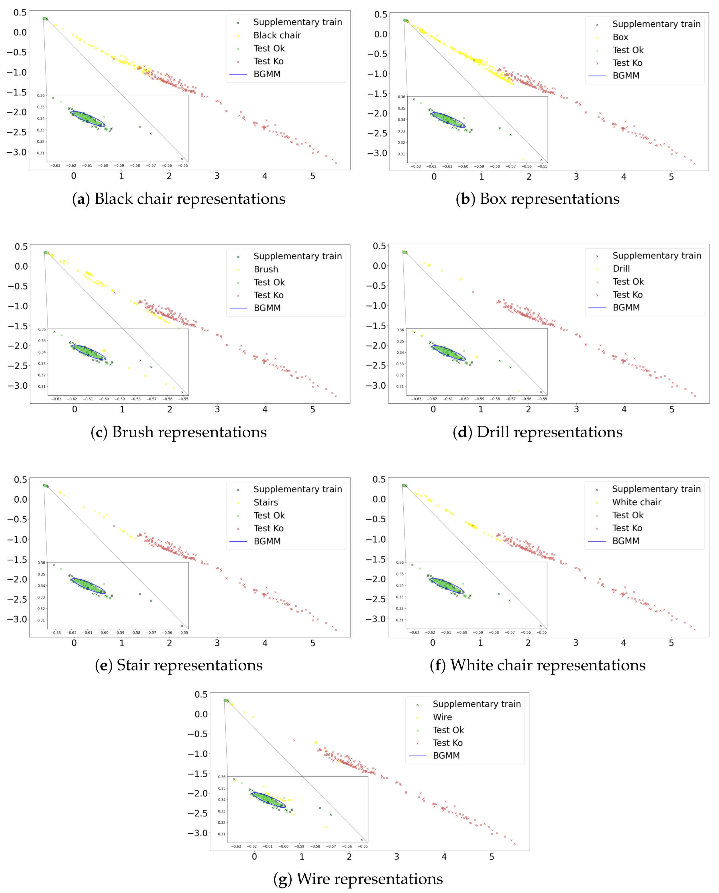
The first step to quantify the performance of the scheme when facing uncertainty is to compute the latent-space representations of the scenarios belonging to the Other objects category. We will only plot the results for the best-performing model, which is ResNet-18, as will be discussed later. These results can be seen in Figure 11. Each of the seven subfigures shows, respectively, the representations obtained for the scenarios with the presence of each of the seven anomalous objects (described in Table 1). Similarly, each subfigure also shows the supplementary train and the Ok-Ko test set representations (the same as Figure 9a). The general trend indicates that the representations of the scenarios with potential safety risk are projected in regions far away from the cluster of Ok observations, namely in an intermediate region between the Ok and Ko representations. Although these anomalous scenarios often present very small deviations from a correct situation, the proposed CL methodology is able to detect and focus on the unknown features that do not characterize the safe scenarios.
Once we have these representations, the second step consists of fitting the BGMM on the projections of the supplementary train dataset. The fitted mixture corresponds to the blue ellipse in Figure 11. To represent this ellipse, we use the mean, covariance, and shape of the estimated supplementary train distribution in the latent space. A closer look at the fit reveals that it is not influenced by the presence of some small outliers (belonging to the supplementary train set). Such robustness implies that the vast majority of representations of the Other objects category lie outside the ellipse that characterizes the estimated distribution, which will result in a high success rate in detecting the unknown scenarios.
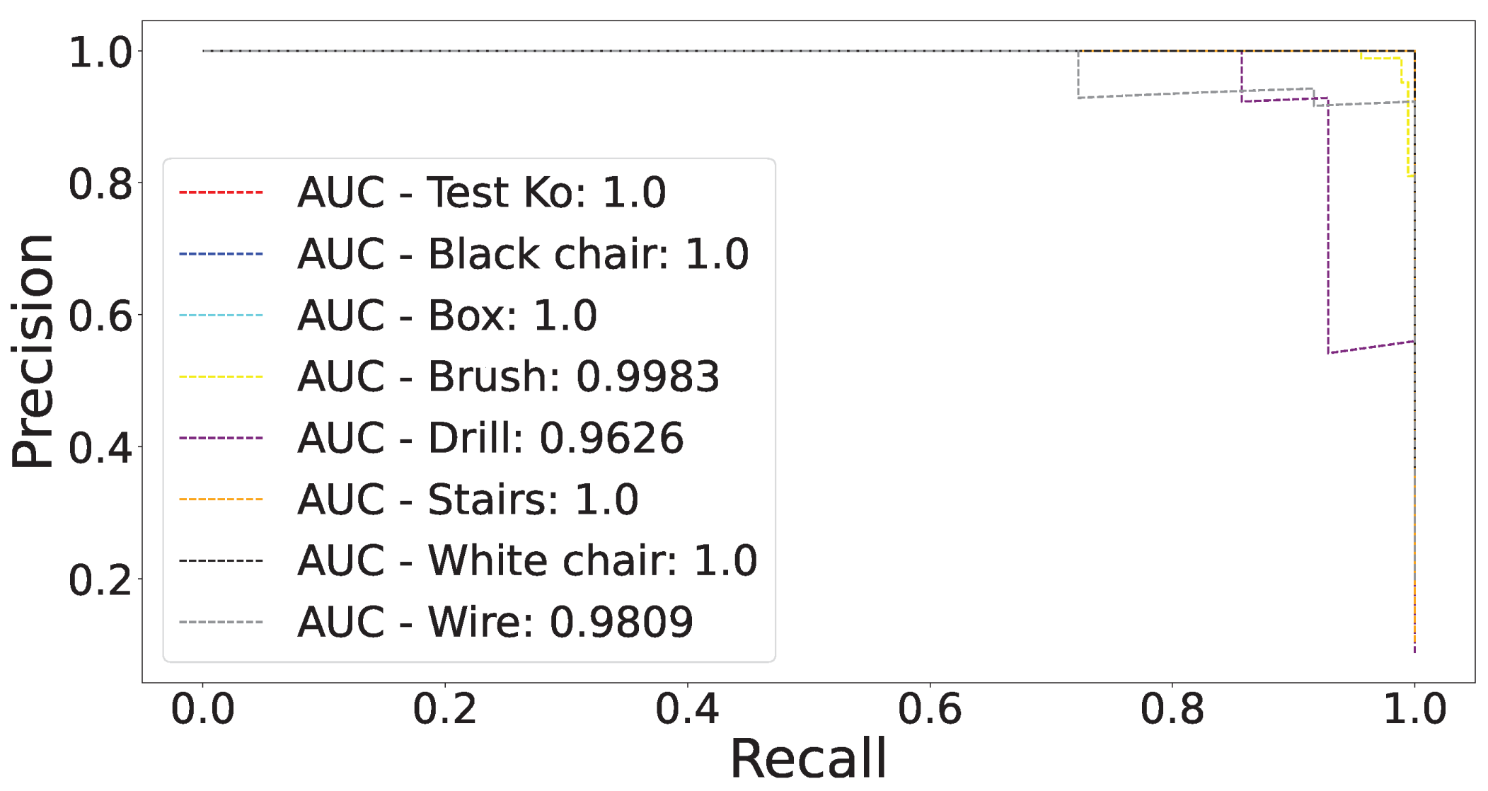
As argued in Section 5.1, in order to quantify the performance of the models, we will identify anomalies by computing the log-likelihood that each observation could have been generated by the BGMM. Using these log-likelihoods we can build, for each anomalous object, a precision–recall (P–R) curve showing the model’s ability to distinguish between safe and potentially unsafe scenarios caused by the concerned object. We use a P–R curve instead of a more straightforward metric, such as accuracy, because the former is much more robust to class imbalance and allows visualizing the tradeoff between the cost of type-I and type-II errors. Since P–R curves focus on the performance of the positive class (class with the highest scores), it is necessary that this becomes the class that captures unsafe or potentially unsafe scenarios. Otherwise, the results would be biased by the safe class and would not be focused on anomalous situation detection. For this purpose, we need to invert the obtained log-likelihood scores. After this simple transformation, observations with a low probability of being generated by the BGMM will have high associated scores, while observations with a high probability of being generated by the BGMM will have low scores. Thus, false positives represent situations where a safe scenario is identified as unsafe, and false negatives represent situations where an unsafe scenario is identified as safe. The P–R curves, and their areas under the curve (AUCs), obtained for the best-performing model on the test set are shown in Figure 12. Each P–R curve represents the binary problem of discerning between the test safe (Ok category) and unsafe (Ko category) or potentially unsafe scenarios (seven curves, one for each anomalous object present in the Other objects category). Performing the same process, the AUCs obtained for all the models are shown in Table 4. It can be appreciated that the ResNet-18 encoder is the one that achieves the best results, with a mean AUC of 0.9928. It is able to identify as unsafe all scenarios where four of the seven anomalous objects (black chair, box, stairs, and white chair) are found. For the scenarios with the presence of the other three anomalous objects (brush, drill, and wire), the AUC is considerably higher than 95%. These results reflect the great ability of the CL-BGMM methodology to derive the characteristics that define a correct scenario and identify any uncertain variation, however small, as a situation that carries a potential safety risk. For the other results, the overall performance of the different encoders is very good when the anomalous objects cover a relatively large proportion of the image pixels (black chair, box, stairs, and white chair). As the strange objects gradually decrease in size, some of the models lose the ability to discriminate from the safe scenes. This behavior aligns with the desirable situation in an industrial deployment since, the smaller an anomalous object found illegitimately in the cell, the more likely it is that it will not constitute any safety or feasibility risk to the manufacturing process.
It is worth noting that the reported results are very high, particularly when differentiating between safe and unsafe situations (person). As discussed in [40], the use of many positive (safe) examples and many negative (unsafe) examples makes it relatively easy to achieve state-of-the-art performance for binary classification problems using supervised contrastive learning techniques. In this work, we have a balanced dataset of around 6000 safe and unsafe images (see Table 1), which enables performing a balanced and precise learning process. In addition, an industrial safety system must offer extremely high performance for the protection of humans. Regarding anomaly detection, due to the quality of the supervised training process, the models are able to synthesize the presence and location of permitted elements and magnify the presence of any unknown deviations in the industrial process.

5.3. Hybrid Latent Space for Performance Maximization

The results presented in Table 4 show considerable oscillations for some categories. Mainly, these are the ones that represent the presence of small objects that barely alter the safe state of the cell (brush, drill, and wire). This variance arises from training with different architectures (CNNs of different families and complexity and a vision transformer) and a CL methodology fed by randomly augmented images. Thus, each model learns to synthesize a different set of high-level features from the data, achieving highly diverse results. This diversity allows exploiting the concept of ensemble learning in order to maximize the overall performance of the pipeline. Ensemble learning refers to the methodology that combines two or more baseline models in order to obtain improved performance and better generalization ability than any of the individual base learners [59,60].
In this work, we propose to use ensemble learning as an intermediate phase between CL training and the Bayesian mixture fit. This process is composed of two different stages. In the first stage, we combine the results coming from two different CL schemes. The selected aggregation mechanism is the concatenation. This process is illustrated in Equation (3), where h θ 1 x i and g θ 1 x i represent two different R 2 latent-space representations of the observation x i , ‖ the concatenation operation, D the dataset, and R the set of representations in a R 4 latent space. The reason for concatenating individual latent spaces to form a latent space of higher dimensionality is to leverage the strengths of each individual model for those categories where it performs best while mitigating potential discrepancies. We assume that an individual model is able to project scenarios with the presence of a specific anomalous object far away from the cluster of safe scenarios, so, when combined with another model, this discriminative power is transferred without perturbations to two of the dimensions that compose the four-dimensional latent space. If the second model is also able to project such scenes away from its safe-scenario cluster, then there will be a clear separation in the two groups of dimensions of the compound latent space. Alternatively, if the second model performs poorly for that category, the compound latent space still maintains high discriminative ability in two of its dimensions, it being highly probable that the remaining dimensions hardly impair the separation transferred by the first model. The second stage remains the same, consisting of adjusting a Bayesian mixture to the safe representations of the R 4 latent space. As previously described, we employ the supplementary train dataset to perform the BGMM fitting and compute the inverse log-likelihood scores of the test set scenarios (Ok, Ko, and Other objects).
R = h θ 1 x i g θ 1 x i | x i D
The results of the hybrid latent-space proposal can be found in Table 5. We have selected a collection of seven cases where a varied casuistry is collected: combinations of base learners where both have good performance (ResNet-18 and DenseNet-201), combinations of base learners where a top-performance model and a model with notably lower performance are used (ResNet-18 and DenseNet-161, DenseNet-201 and DenseNet-161, and ResNet18 and ConvNeXt-nano), and combinations of base learners where the performance of both models is relatively low (the remainder).
Analyzing the results from a general perspective ( AUC mean ), the main point that can be noticed is that, for all cases, the hybrid model improves the results of the best base learner that participates in the combination. By category, the main improvement in the results can be observed in small objects, which are the most difficult to detect. For the drill category, all seven combinations exceed the performance of their base models. In the case of the brush and wire categories, six of the seven combinations achieve an improvement. In the case of the box and stairs categories, the only combinations that can improve the results do so. For all other categories, when the results of the base learners are perfect, the hybrid model maintains the performance. Analyzing the results regarding the type of combination, it is worth noting that the effectiveness of the method is robust to the underlying performance differences between the models that are combined. For example, when combining two high-performance models (see ResNet-18 and DenseNet-201), the ensemble approach achieves improved results in the only categories where there is room for improvement (brush, drill, and wire). The features learned by both encoders vary, and their combination allows taking advantage of the situations where each one performs best to obtain a high-dimensional latent space where even the most complex illegitimate variations are separated from the safe-scenario cluster. Remarkably, the observed behavior occurs in cases where two models with different performance are combined (see ResNet-18 and ConvNeXt-nano). The features learned by the simpler model provide discriminative capabilities to the information encoded in the latent-space distribution generated by the more complex encoder, inducing a combination that maximizes performance. Finally, when two models with lower performance are combined (see ConvNeXt-nano and EfficientNetB0), the ensemble allows for improved performance in detecting scenarios belonging to the most complex categories.
The best hybrid model obtained (ResNet-18 and DenseNet-201) has almost perfect behavior. In addition to detecting with perfect accuracy all unsafe scenarios due to the presence of people, it is also able to detect all potentially unsafe scenarios caused by the presence of six of the seven unknown objects. The only potentially unsafe scenarios that it is not able to fully detect are those where strange wires are present. We note that this anomalous object is particularly difficult to detect as a multitude of correct scenarios present wires in a wide range of positions (driven by the movement of the robotic arm) that do not compromise the safety of the industrial process. Even so, the AUC is practically perfect, with a value of 0.9874, reflecting that a very high proportion of these scenarios are differentiated from the cluster of safe scenarios.

6. Confidence Against Uncertainty: Explainable Artificial Intelligence (XAI)

The proposed methodology based on CL and Bayesian mixtures is able to determine very effectively when the industrial cell is in an unsafe state, either by the presence of a person (see Section 4) or any type of unknown object that may potentially compromise the integrity and reliability of the manufacturing process (see Section 5). Beyond the results, the application of AI-based methods in a safety-related domain requires a high level of confidence in their decision-making process, as well as an understanding how they will behave when faced with unknown situations that may arise in the future. With the aim of providing confidence and understanding the decisions made by AI models, the field of explainable artificial intelligence (XAI) has recently come to the forefront. XAI is a term that refers to AI systems that can provide explanations for their decisions or predictions to human users [61]. This process becomes crucial in some domains, specifically in the safety field (see [61]). Most existing research on XAI focuses on providing a comprehensive overview of approaches for either explaining black-box models or designing white-box models [62], the former being the focus of this work. The BGMM phase is highly interpretable and does not require any auxiliary process to unravel the underlying mechanism that regulates its behavior. Therefore, we will focus on identifying the factors that determine the decisions made by the DL encoders trained with CL. In particular, we will study which regions of the scenarios cause them to be projected at a point near or far from the cluster of safe scenarios in the latent space. To this end, we will employ two techniques. The first one, proposed in this work, is based on ablations of the initial feature space, while the second one, more conventional and widespread for the diagnosis of computer vision models, is the computation of saliency maps.

6.1. Input Feature Ablations

Ablations, in the context of an AI application, consist of removing one or more of the components that comprise the system and examining how this affects the final behavior. Commonly, ablation studies involve adding or removing components from a model (see [63,64]). However, ablations can also be performed on the data that serve as input to the models in order to study how their perturbation impacts the performance. For example, data ablations are used in [65] in order to remove repeated patterns in images and test whether deep neural networks can maintain a high level of confidence in their predictions. In [63], the concept of data ablations is fully exploited, developing a tool that enables conducting studies for general computer vision problems. In [66], the randomized ablation feature-importance technique is introduced, where the different input characteristics (independent variables of a dataset) are replaced by a random variable with a marginal distribution according to the original variable, checking for each replacement whether the model’s ability to make a good prediction is preserved.
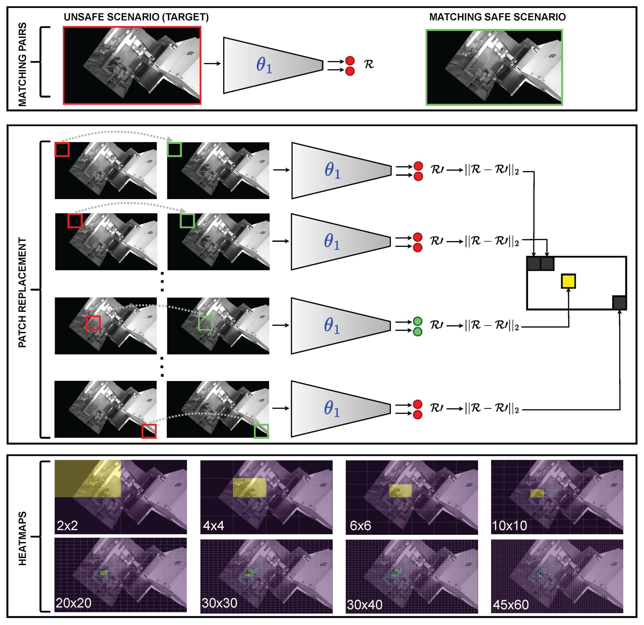
In this work, we design a novel patch-based input-feature-ablation method inspired by the work presented in [66]. Instead of randomly perturbing portions of the initial feature space that feeds the DL models, we perform a similarity-based search on the dataset image and replace the patches with others that are geospatially consistent. A visual representation of the developed ablation pipeline can be found in Figure 13. The first step consists of selecting two scenarios: the one in which the ablation study will be performed (target scenario; typically unsafe or potentially unsafe) and a scenario as similar as possible to the one to be ablated belonging to the cluster of safe scenarios. This matching is feasible in our use case since it is highly probable that, for each unsafe scenario, there is an almost identical safe configuration in which the only difference is the absence of the element that triggers the unsafe state of the cell. The reason for this matching is that partial parts (patches) of the target image will be replaced by the equivalent parts corresponding to the safe counterpart. Thus, it is possible to generate a much more realistic ablation than would be achieved by replacing the patches with black regions or by randomly filling the pixels. For each of the patch substitutions, and until the entire image is covered, the latent-space representation is computed, measuring the deviation produced with respect to the original target representation.
The deviation computation is written in Equation (4), where x represents the target image, p x represents the function that performs the process of replacing a patch in x, and d is the deviation. Therefore, if a patch replacement results in a high deviation with respect to the target representation, it means that the DL scheme was extracting relevant features from the target patch, which caused the scenario to be projected in a region far away from the safe-scenario cluster. In contrast, if the ablation barely affects the latent-space representation, it means that the corresponding portion of the cell did not contain any significant feature that was determinant in projecting the scenario in the unsafe region. The smaller the size of the patches, the more detailed the information about which areas of the cell contain information relevant to the encoders. Finally, with the deviation computed for each patch, we can build a heatmap that displays which patches cause more deviations and which patches are more irrelevant to the decision taken by the model (the more important, the stronger the yellow color).
d = | | h θ 1 x h θ 1 p x | | 2
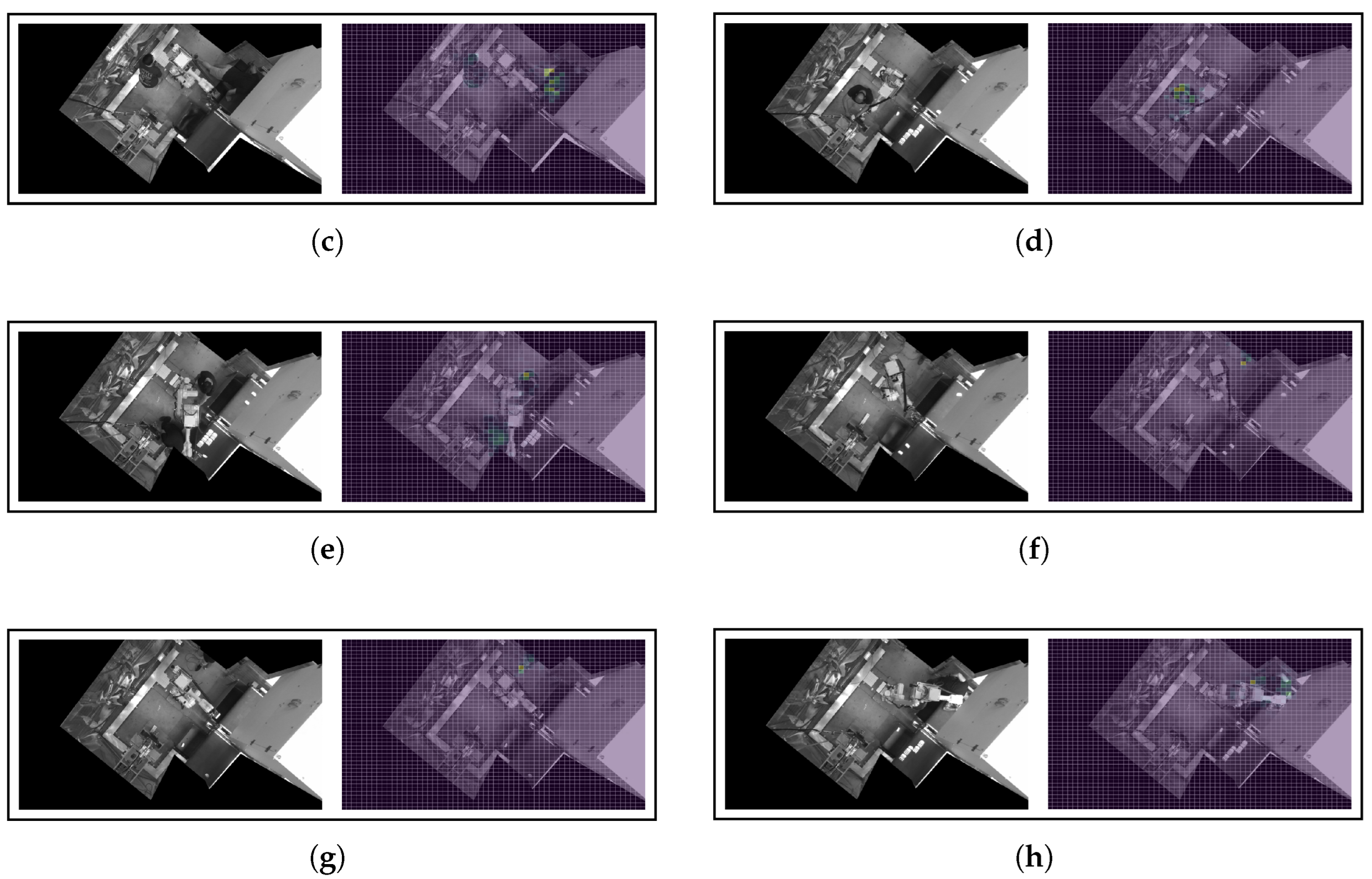
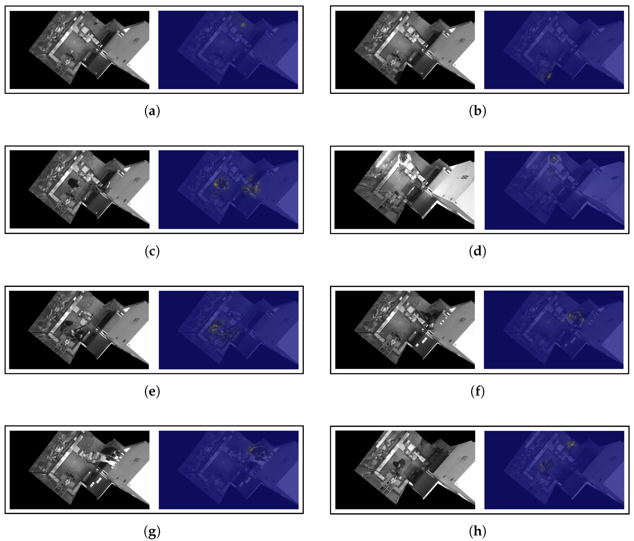
Figure A2 (see Appendix B.1) shows the ablation results obtained for eight Ko observations of the test set using the best individual model (ResNet-18) and a 45 × 60 patch grid. We have selected a varied set of scenarios that are representative of different interactions that humans may have with the manufacturing cell. There are some scenarios where several workers are within the cell (Figure A2a–c,e), where only small parts of workers are visible (Figure A2b,f,g), and where some workers are partially covered by the machinery (Figure A2c,h). All these situations have been captured during the setup and fine-tuning of the industrial process and are highly likely to be repeated during the life cycle of the machine. Therefore, it is essential to ensure that the decisions made by the DL models are fully justified and without biases that may induce inconsistent behavior. A close analysis of the heatmaps obtained using the input-feature-ablation technique shows that, in all cases, the patches with a more intense yellow color are those close to the place where the workers are located. As already argued, this means that these patches have the greatest influence on the encoder in projecting the corresponding images far away from the cluster of safe scenarios. Even in the most challenging situations, where only a part of a person’s foot is visible (Figure A2f) or the person is partially covered by the robotic arm (Figure A2h), the DL model is able to very accurately detect the small deviations that exist with respect to the set of Ok scenarios. It is also remarkable that, in the case of scenarios with multiple workers, the DL model is able to detect the presence of all foreign bodies remaining in the cell. The decision to move such scenarios away from the safe cluster is equally influenced by pixels belonging to different humans. This behavior shows that the model lacks biases whereby it is influenced more by individuals, or parts of individuals, of greater size.
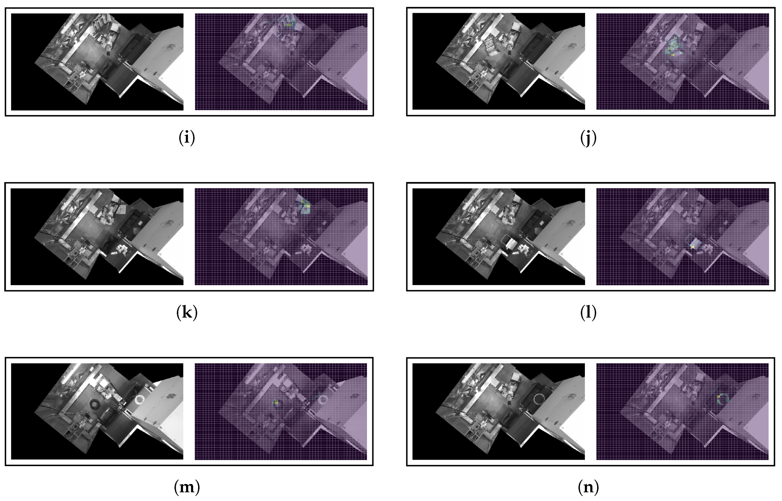
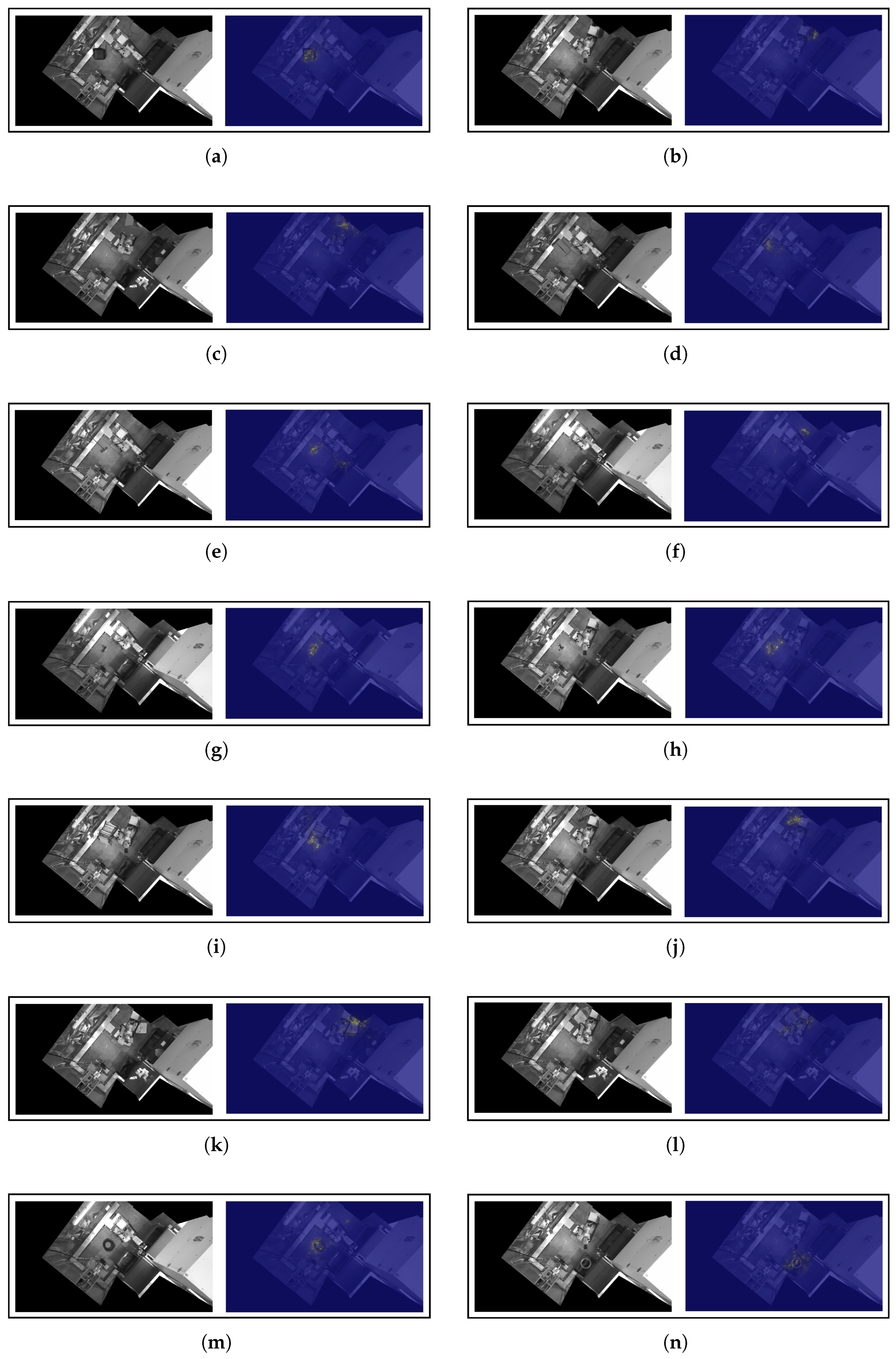
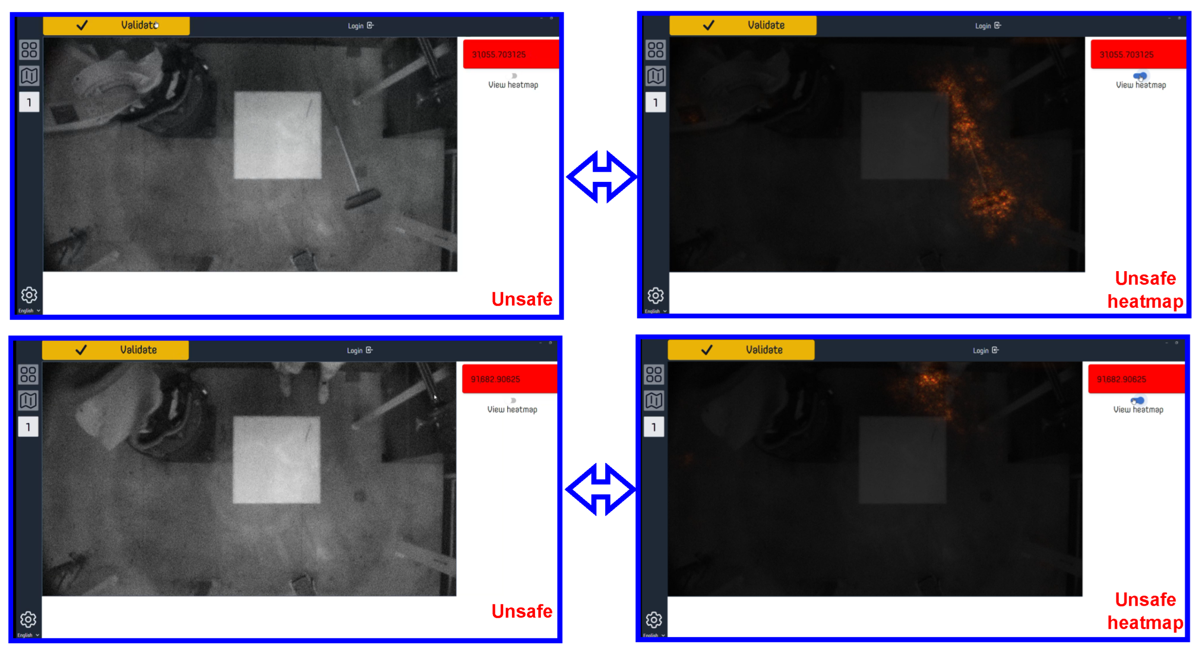
Similarly, Figure A3 (see Appendix B.1) shows the result of applying the input ablations to a set of scenarios belonging to the Other objects category. Two representative scenarios have been selected for each of the anomalous objects contained in the aforementioned category. Note that the patches that induce a greater deviation of the representation in the latent space are mostly concentrated in the areas adjacent to unknown objects. It is worth pointing out the case of Figure A3h, where the anomaly is caused by a small object (drill) partially covered by the robotic arm. Despite the complexity of identifying the anomaly, the model is able to determine the presence of a foreign body outside the set of patterns that characterize safe scenarios. Another highly complex scenario is Figure A3n, where an anomalous object (wire) is placed above one of the conveyor belts of the cell. The surface of the conveyor belt exhibits great variability within the set of Ok scenarios since there is virtually unlimited casuistry in the disposition of the transported parts. However, rather than decreasing its performance in the aforementioned area, the DL model is able to determine the presence of a morphology different from those that are commonly carried by the conveyor belt. Thus, the input feature ablations illustrate the effectiveness of the proposed scheme to detect any type of anomalous object and, therefore, to be robust and provide guarantees of high performance in the event of uncertain conditions. More examples of the heatmaps produced by this methodology can be found on our GitHub (see github.com/jesusferigl/ (accesed on 6 November 2025)).
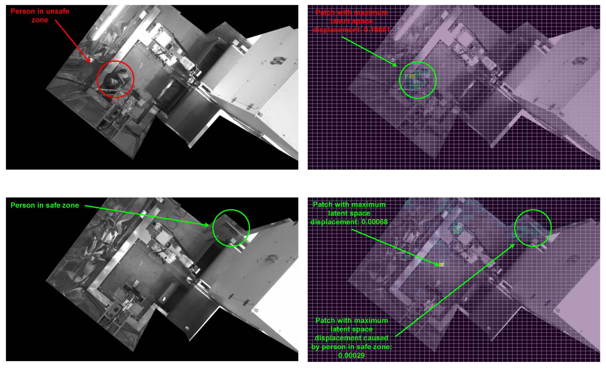
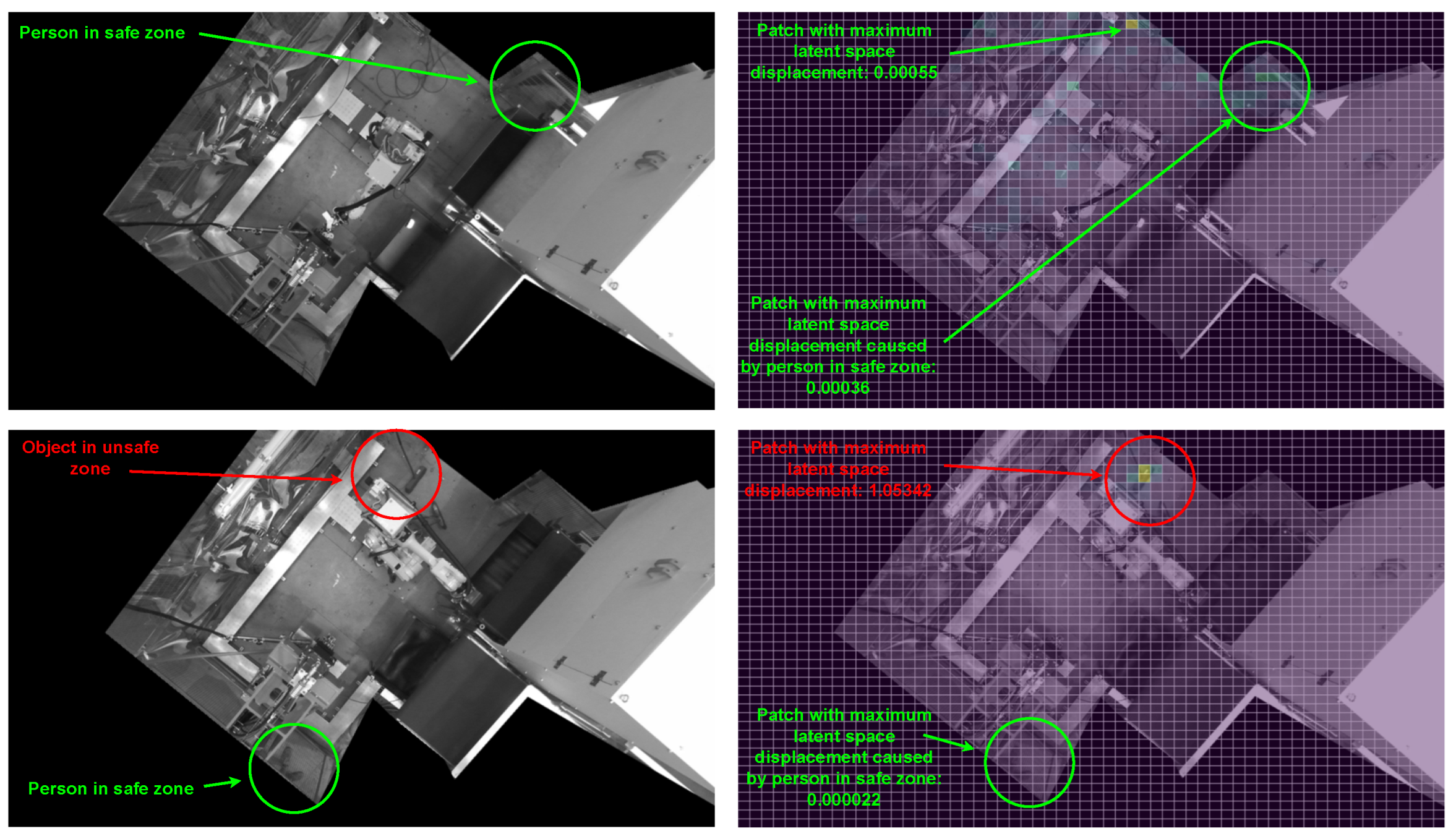
From an industrial deployment perspective, the input-feature-ablation method will only be applied when the AI-based safety channel has detected an unsafe scenario. However, it is also useful to use this method to determine whether the model is capable of ignoring the presence of persons or other objects in areas outside the facility but visible in the images. Thus, we can guarantee that the variability in the environments surrounding the cell will not cause false positives and, therefore, unnecessary production stoppages. The analysis performed is shown in Figure A4. Four test set images representative of the case study have been selected. The first image shows a person inside the facility, the next two Ok images show people working in the surroundings of the facility, and the last image shows both an anomalous object inside and a person working outside. In the image with a person inside, the maximum displacement (Euclidean distance) caused in the latent space by the replacement of the patch belonging to the person has a magnitude of 0.1881. Similarly, in the image with an object inside (brush), the displacement caused by the associated patch is 1.0534. In the same image, a person is outside the facility, and the displacement caused by replacing their patch with a patch without a person is 0.000022. In the two Ok images, the patches associated with people outside the facility cause displacements of 0.00068 and 0.00055. These displacements are several orders of magnitude lower than the ones caused by real unsafe or potentially unsafe scenarios, showing that the models are capable of omitting the presence of people and, in general, variable situations outside the cell. This ensures that the AI safety system will not block the manufacturing process due to external false positives.

6.2. Saliency Maps

A widely used technique to explain the decisions made by DL models involves saliency maps. This technique, presented in [67], belongs to the family of gradient-based methods (see [68]) and relies on the calculation of the gradient of the final prediction with respect to the input of the network. This gradient represents how each input variable contributes to the output prediction. As such, gradient-based methods generate heatmaps that indicate the importance of each pixel in the input space to the network’s final prediction [69]. Saliency maps were originally designed from the perspective of a classification paradigm, estimating the areas of the image that were most important in order to assign the input to a particular category (see [67]). Typically, the backpropagation-based computation of the gradient starts from the neuron associated with the class that has obtained the highest score. However, in this work, DL models belong to the CL paradigm, so the target of the final layer is not the same as in a classification scheme. Each neuron in the last layer represents one of the two dimensions of the latent space into which the inputs are projected and does not compute a score associated with a classification approach. Therefore, when choosing which neuron should start the gradient computation, it would not be correct to select the one that computes a higher value (which would be the case in a classification problem as the higher value would represent the most likely class). To overcome this, we propose to always choose the same neuron, namely the one associated with the dimension of the latent space that gathers as much variance as possible. This dimension will have higher discriminatory power, so it is more likely that its backpropagation will obtain the most relevant saliency maps, showing the image characteristics that determine whether it belongs to the safe cluster or not. Regarding the best single model (ResNet-18), this dimension corresponds to the first one (x-axis in Figure 11). Thus, to compute the saliency maps, we will always use the neuron associated with the x-dimension of the latent space as the starting value for the backpropagation.
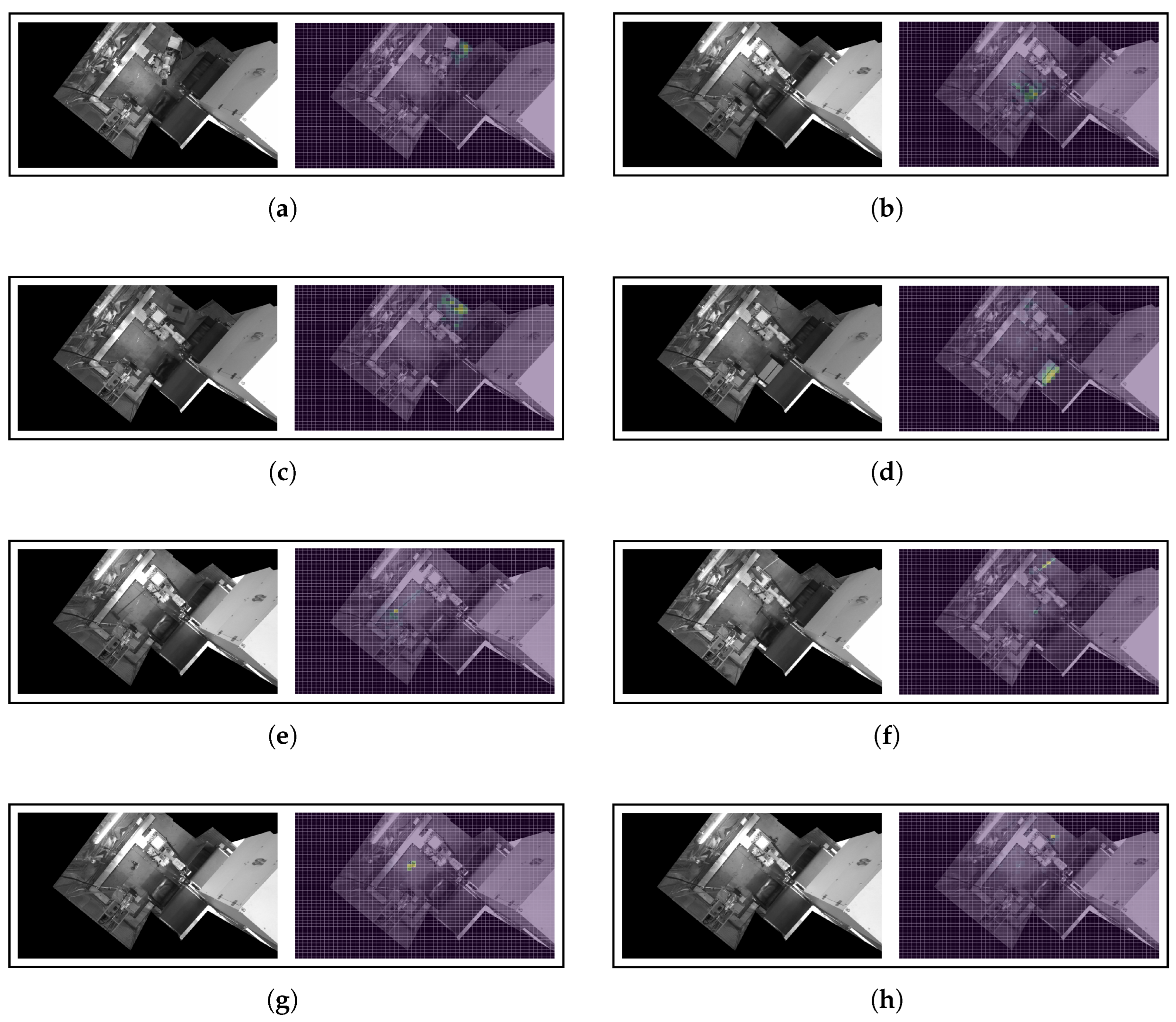
In Appendix B.2, Figure A5 and Figure A6 show the results obtained for a test set sample of the Ko and Other objects categories, respectively, using the best single model (ResNet-18). As with the previous XAI technique, we have selected a set of representative scenarios that cause the cell to fall into an unsafe state. Analyzing the scenes with the presence of humans (Figure A5), it can be appreciated that the regions with the greatest importance in projecting the scenarios far from the safe cluster are those where the workers are located. As already shown using the input feature ablations, this behavior is consistent regardless of the size of the person. In Figure A5a, the network is able to base its decision on the presence of a person’s leg. Similarly, in Figure A5b, the DL model detects that the disturbance of the safe scenario comes from the presence of a body part of a person. In Figure A5c,h, the regions with the greatest influence on the input come from both a complete and a partial body, showing the robustness of the proposed scheme regardless of the human morphology. Likewise, the model is able to draw its judgment from information coming from different areas.
Regarding the scenarios where unknown objects are found (Figure A6), the results derived from computing the saliency maps are satisfactory. The technique reveals that the portions of the image that condition the network decisions are those with anomalies. It is worth highlighting some challenging situations, such as in Figure A6b, where the black chair is almost entirely covered by the robotic arm yet the DL model is able to identify the slight unknown disturbance in that area. In Figure A6e, the scheme bases its decision on the identification of two foreign bodies (brushes) whose characteristics are not representative of the normal operation of the manufacturing process. We note that one of these brushes is extremely difficult to detect (the one on the right), both because of its small size with respect to the cell and because it is just located in the area of the conveyor belts and the containers where the parts that the robot fails to pick up fall. Despite the set of Ok scenarios containing high variability of situations in the aforementioned area, the DL model is able to detect that the morphology of the brush, although extremely fine, diverges from the morphologies that may appear in that zone during a correct operation state. This case is similar to the one reflected in Figure A6n, where, even though a wire is placed in the container where the parts of a conveyor belt may fall, the DL model is able to determine that there is an unknown morphology. In Figure A6m, the two areas with presence of anomalous wires influence the results provided by the network. This case is highly complex to detect as there are certain allowed robot wire patterns around those areas contained within the set of safe scenarios.

6.3. Discussion

Overall, the results obtained using the proposed patch-based input-feature-ablation method are consistent with the ones obtained using the saliency maps, reflecting the high quality of the predictions. The proposed CL scheme is able to synthesize and base its decisions on the non-legitimate disturbances of the industrial cell, whether known (people: Ko) or in the face of uncertainty (anomalies: Other objects). Consequently, the Bayesian mixture is indeed able to very accurately quantify the deviation that each non-legitimate situation entails from the set of characteristics that determine the safe scenarios. The XAI techniques presented in this work ensure that the proposed scheme is free of biases that may distort the obtained results and, therefore, lead to long-term inconsistent behavior when deployed in an industrial plant. Likewise, we show that DL models will perform properly when dealing with any abnormal event not covered during their training phase. In addition, the feature-ablation method demonstrates that the presented methodology is capable of ignoring the presence of illegitimate elements in areas outside the monitored perimeter, even when they are visible in the images. This ensures that the system will not decrease its performance when the environments surrounding the industrial cell vary. The proposed pipeline provides guarantees to successfully manage the uncertainty that may arise in advanced manufacturing environments. Also, the heatmaps generated by the XAI methods can be integrated into a software application to help operators identify unsafe areas in industrial facilities (see Section 7), thereby improving the usability and transparency of the safety system decision-making process.

7. Industrial Deployment

In this section, we detail the characteristics of the industrial deployment that has enabled us to carry out the experimentation described in the work and assess the performance of the system in a real production environment. Similarly, we will also describe the main limitations encountered in the study, as well as the new lines of research that are already being developed. The pipeline based on CL and Bayesian clustering has an average inference time of 50 milliseconds using an industrial PC (IPC; see characteristics in Section 3.4). This implies that, on average, the AI auxiliary safety channel will deliver outputs at 20 frames per second (FPSs). The speed of the method allows it to be used in two different operating modes:
  • Cycle-triggered-monitoring mode: the system will diagnose the safety of the industrial space only at the start of each production cycle.
  • Continuous-monitoring mode: the safety check will be performed periodically every 50 milliseconds.
Both operating modes are meaningful depending on the layout of the monitored cell and the safety devices already integrated. For instance, in a completely fenced-off cell whose only access point is an industrial door, checking for the presence of unauthorized elements at the cycle start is enough since, once started, the safety chain of the installation cannot be broken unless the door is opened. On the other hand, a cell in which the operator can load components or access the machinery during the cycle benefits from the AI safety system continuously checking the legitimacy of the process. In the industrial configuration described in Section 3.1, data has been collected and the system evaluated using captures during the active industrial cycle, i.e., continuous-monitoring mode. The reason is that the machine has two entry and exit points (conveyor belts) through which an untrained or malicious worker can easily access the interior of the facility and throw unexpected objects. The programmable logic controller (PLC) used is a Siemens SIMATIC S7-1200F safety CPU with eight digital inputs and six digital outputs. We also use a Siemens SIMATIC S7-1200 digital I/O module, Relay Output SM 1226 with PROFIsafe, for communication between the digital outputs and the facility’s actuators (robot, welding press, and conveyor belts). This module enables sending the stop signal when the safety circuit is broken. To communicate the IPC with the PLC, a digital I/O card connected via Ethernet to the IPC is used, which also interfaces with a safety-rated digital input module of the PLC. In addition, the PLC implements a watchdog system that determines whether the IPC is active by checking whether a bit in its DB is modified every 20 milliseconds. When the AI safety channel detects any non-legitimate situation, the software running in the IPC displays on a monitor an image generated using input feature ablations (see Section 3.1) to help workers diagnose what is triggering the safety alert. Figure 14 shows an example of the software program that has been built to integrate the methodology presented in this work. The monitored installation is different from the one discussed previously as, for confidentiality reasons, screenshots of the final deliverable deployed in the industrial plant cannot be published. When an unsafe scenario is detected, the machine operator, through a touch screen, can use a toggle button to view a heatmap showing where the anomaly is located. This map is computed using the input-feature-ablation technique detailed in Section 6.1.

Limitations and Future Work

Three main limitations have been identified that need to be addressed in future research. The first one is the possible sensitivity to the general lighting conditions of the facility. Generally, all DL algorithms, even when trained with data augmentation that distorts the color space (brightness, saturation, contrast, etc.), tend to overfit the underlying lighting conditions in the training datasets. The industrial belt-picking cell monitored in this study has an LED lighting system that provides homogeneous illumination across the cell surface. However, at the end of the luminaires’ useful life or in the event of an unexpected error, lighting conditions may deteriorate and affect system performance. Moreover, if the machine is located in an industrial plant with large windows, direct sunlight can cause glare or saturation that may distort the AI results. As detailed in Section 3.2, in this work, we have captured images with varying lighting conditions, both environmental (different days and times of day) and different power levels in the LED lighting, to achieve more robust training of the models and more representative results. However, we believe that this point requires further attention and long-term testing on different machines and industrial plants to ensure robustness in the face of all types of lighting variations. In parallel, Aparicio-Sanz et al., in prep., will propose near-infrared (NIR) lighting and NIR-sensitive cameras that isolate the vision system from the lighting conditions in the plant.
The second identified improvement is related to rapid deployment on new machines or ease of adaptation to layout changes. Since reconfigurable manufacturing systems (RMSs) are becoming increasingly prevalent in advanced industry, the associated safety systems must also be simple to use and not require tedious parameterization. The importance of these reconfigurable safety systems (RSSs) is discussed in [36,70]. Currently, the proposed CL-based method has been trained in a supervised manner using images representing the machine in a safe state (normal production cycle) and an unsafe state (workers performing maintenance tasks within the facility and tricky situations forced to evaluate the method’s performance). This implies that, in case of a machine layout change, it would be necessary to recapture the set of safe and unsafe scenes. Although safe scenes are easy to record (normal production cycle), unsafe scenes require time and effort. To solve this problem, Aparicio-Sanz et al., in prep., will propose a methodology derived from the one presented in this paper called human augmentation, which allows for plug-and-play operation in a new installation or when changing an existing layout.
The last limitation detected in this work, and a point to consider for future research, is the number of anomalies gathered in the dataset and their size. As can be seen in Table 1, the number of images captured with anomalous elements is much lower than the number of Ok and Ko images. The reason for this is the difficulty and danger of introducing such objects into an industrial production process. Therefore, it is useful to validate the accuracy of the system with a broader set of anomalies. In parallel, as seen in Section 5, when anomalous objects become smaller, the effectiveness of the safety system decreases slightly. In this study, a 2 MPx camera was used to monitor the installation, resulting in a pixel size of 4 mm 2 . Therefore, there is a risk that, when small but dangerous anomalous objects (lighters or pieces of cloth) are placed within the facility, the safety system will not be able to detect them. The use of high-resolution industrial cameras or the parallel analysis of information from several cameras will be necessary to avoid such situations.

8. Conclusions

In this work, we create a DL system based on CL and Bayesian analysis that improves the safety conditions achieved through the application of traditional functional safety devices in industrial manufacturing cells. Using data from an automated press welding cell fed by a belt-picking process currently in production, we develop a DL methodology to discriminate between safe and unsafe scenarios, the latter characterized both by the presence of people and anomalous objects. First, using a supervised deep CL framework, we obtain robust latent-space representations by maximizing the distances between safe and human-present scenarios. Second, fitting a Bayesian Gaussian mixture to the learned latent-space distribution, we robustly synthesize the underlying trend of the safe representations, detecting those scenarios whose features deviate from safe behavior, i.e., scenarios with the presence of non-legitimate elements. We obtain a perfect AUC for discriminating between safe and human-present scenarios, and an average AUC of 0.9982 for discriminating between safe scenarios and scenarios with seven types of anomalous objects that have not been seen during training. Hence, in addition to reliably identifying human presence, we are able to detect any kind of anomalous object even without having been involved in the learning process of the DL model. Furthermore, by combining different DL schemes through the generation of ensemble-based hybrid latent spaces, we are able to join the discriminating features of the underlying models and maximize the overall performance. In order to provide confidence in the achieved results and gain insights into the decision-making process, an explainable artificial intelligence analysis based on two different techniques is carried out. Specifically, we suggest using saliency maps and an innovative technique based on patch-based input feature ablations that we design for this purpose. We show that the proposed methodology is solid, consistent, and without biases that may distort the results and lead to long-term inconsistent behavior. Thus, we guarantee that the models will detect and react appropriately to the occurrence of any type of unknown situation, being able to manage uncertainty. The main limitation of this work is scalability. Deploying the safety system in a new facility requires recording, beyond the normal production cycle, human-involved scenarios that represent unsafe conditions. This data collection is both risky and time-consuming, hindering rapid and transparent scaling. Robustness against unexpected lighting changes and having a larger set of anomalies should also be addressed in future research. The combination of techniques developed in the work has been successfully deployed and is currently undergoing validation in a real industrial production environment. To the authors’ knowledge, this is the first work to propose and validate the development of an AI-managed safety channel that improves upon, and can be combined with, the capabilities offered by traditional functional safety measures, which represents a significant breakthrough in the efficiency, reliability, and safety of modern industrial processes.

Author Contributions

Conceptualization, J.F.-I., F.B. and B.S.; methodology, J.F.-I. and B.S.; software, J.F.-I.; validation, J.F.-I., F.B. and B.S.; formal analysis, J.F.-I.; investigation, J.F.-I. and B.S.; resources, J.F.-I., F.B. and B.S.; data curation, J.F.-I.; writing—original draft preparation, J.F.-I., F.B. and B.S.; writing—review and editing, J.F.-I., F.B., and B.S.; visualization, J.F.-I.; supervision, F.B. and B.S.; project administration, J.F.-I.; funding acquisition, J.F.-I. and F.B. All authors have read and agreed to the published version of the manuscript.

Funding

Consolidación Investigadora IGADLE project with reference CNS2024-154572.

Informed Consent Statement

Informed consent was obtained from all subjects involved in the study.

Data Availability Statement

The datasets generated and analyzed during the current study, as well as the training scripts, are not publicly available due to the fact that they constitute an excerpt of research in progress but are available from the corresponding author on reasonable request.

Acknowledgments

The authors acknowledge WIP by Lear and Lear Corporation for collaboration in the project. J. Fernández-Iglesias, F. Buitrago, and B. Sahelices acknowledge support from the GEELSBE2 project with reference PID2023-150393NB-I00 funded by MCIU/AEI/10.13039/501100011033 and the FSE+, and also financial support of the Department of Education, Junta de Castilla y León and FEDER Funds (Reference: CLU-2023-1-05).

Conflicts of Interest

Author Jesús Fernández-Iglesias was employed by the company WIP by Lear. The remaining authors declare that the research was conducted in the absence of any commercial or financial relationships.

Abbreviations

The following abbreviations are used in this manuscript:
AECArchitecture, engineering, and construction
AIArtificial intelligence
ANSIAmerican National Standards Institute
AUCArea under the curve
BGMMBayesian Gaussian mixture model
CLContrastive learning
DLDeep learning
EHSRsEssential health and 46 safety requirements
EMExpectation–maximization
FPSFrame per second
ICSIndustrial control system
IPCIndustrial PC
OSHAOccupational Safety and Health Administration
PaCMAPPairwise controlled manifold approximation projection
PCAPrincipal component analysis
PLCProgrammable logic controller
P–RPrecision–recall
t-SNEt-distributed stochastic neighbor embedding
XAIExplainable artificial intelligence

Appendix A. Overlapping Bell Curves

Figure A1. Overlapping bell curves showing, for each encoder, the Ok and Ko distances from the test set observations to the supplementary train safe cluster. Vertical dashed lines show the minimum and maximum Ko distances. In all cases, there is a clear separation between the distributions of distances corresponding to safe scenarios and those corresponding to unsafe scenarios. The vertical axis has been limited to the range [0, 2] in order to properly appreciate the shape of the Ko distribution.
Automation 06 00084 g0a1

Appendix B. Interpretability Outputs

Appendix B.1. Input Feature Ablations

Figure A2. Input ablations performed on samples from the Ko test set using the ResNet-18 encoder. Yellowish tones represent patches with more impact on the latent-space representation calculated by the model. For each subfigure (ah), the original image is on the left and the resulting output is on the right.
Automation 06 00084 g0a2aAutomation 06 00084 g0a2b
Figure A3. Input ablations performed on samples from the Other objects set using the ResNet-18 encoder. For each anomalous object, two different scenarios are shown (each row refers to the same object, keeping the order of Table 1). Color scheme corresponds to the one used in Figure A2. For each subfigure (an), the original image is on the left and the resulting output is on the right.
Automation 06 00084 g0a3aAutomation 06 00084 g0a3b
Figure A4. Input ablation result for persons and anomalous objects placed in unsafe (inside) and safe (outside) zones of the manufacturing cell. In green font, latent-space displacement when replacing a patch with a person outside the manufacturing cell or a patch that is safe. In red font, latent-space displacement when replacing a patch that is unsafe. The displacement is several orders of magnitude greater when the patch is unsafe.
Automation 06 00084 g0a4aAutomation 06 00084 g0a4b

Appendix B.2. Saliency Outputs

Figure A5. Saliency maps computed on samples from the Ko test set using the ResNet-18 encoder. Yellowish tones represent pixels that make a large contribution to the CL decision-making process. For each subfigure (ah), the original image is on the left and the resulting output is on the right.
Automation 06 00084 g0a5
Figure A6. Saliency maps computed on samples from the Other objects set using the ResNet-18 encoder. For each anomalous object, two different scenarios are shown (each row refers to the same object, keeping the order of Table 1). Color scheme corresponds to the one used in Figure A5. For each subfigure (an), the original image is on the left and the resulting output is on the right.
Automation 06 00084 g0a6

References

  1. Bureau of Economic Analysis Number and Rate of Nonfatal Work Injuries in Detailed Private Industries. Available online: https://www.bls.gov/charts/injuries-and-illnesses/number-and-rate-of-nonfatal-work-injuries-by-industry-subsector.htm (accessed on 3 September 2025).
  2. Eurostat Accidents at Work-Statistics by Economic Activity. Available online: https://ec.europa.eu/eurostat/statistics-explained/index.php?title=Accidents_at_work_-_statistics_by_economic_activity (accessed on 3 September 2025).
  3. Eurostat Gross Value Added at Current Basic Prices, 2005 and 2024 (% Share of Total Gross Value Added). Available online: https://ec.europa.eu/eurostat/statistics-explained/index.php?title=File:Gross_value_added_at_current_basic_prices,_2005_and_2024_(%25_share_of_total_gross_value_added)_NA2025.png (accessed on 3 September 2025).
  4. Bureau of Economic Analysis Value Added by Industry as a Percentage of Gross Domestic Product. Available online: https://apps.bea.gov/iTable/?reqid=1603&step=2&Categories=GDPxInd&isURI=1&_gl=1*132dtfk*_ga*MTQyNTk0ODU2NS4xNzU2OTIwMzg5*_ga_J4698JNNFT*czE3NjQyNjg1NjIkbzIkZzEkdDE3NjQyNjg2MzUkajYwJGwwJGgw#eyJhcHBpZCI6MTYwMywic3RlcHMiOlsxLDIsNF0sImRhdGEiOltbImNhdGVnb3JpZXMiLCJHRFB4SW5kIl0sWyJUYWJsZV9MaXN0IiwiVFZBMTEwIl1dfQ== (accessed on 3 September 2025).
  5. Lee, K.; Shin, J.; Lim, J.Y. Critical Hazard Factors in the Risk Assessments of Industrial Robots: Causal Analysis and Case Studies. Saf. Health Work 2021, 12, 496–504. [Google Scholar] [CrossRef]
  6. ISO 13849-1:2023; ISO Central Secretary. Safety of Machinery—Safety-Related Parts of Control Systems—Part 1: General Principles for Design. Standard, International Organization for Standardization: Geneva, CH, USA, 2023.
  7. IEC 62061:2021; IEC Central Secretary. Safety of Machinery—Functional Safety of Safety-Related Control Systems. Standard, International Electrotechnical Commission: Geneva, CH, USA, 2021.
  8. Fernández, J.; Valerieva, D.; Higuero, L.; Sahelices, B. 3DWS: Reliable segmentation on intelligent welding systems with 3D convolutions. J. Intell. Manuf. 2023, 36, 5–18. [Google Scholar] [CrossRef]
  9. Wu, Z.; Cai, N.; Chen, K.; Xia, H.; Zhou, S.; Wang, H. GAN-based statistical modeling with adaptive schemes for surface defect inspection of IC metal packages. J. Intell. Manuf. 2023, 35, 1811–1824. [Google Scholar] [CrossRef]
  10. Cardellicchio, A.; Nitti, M.; Patruno, C.; Mosca, N.; di Summa, M.; Stella, E.; Renò, V. Automatic quality control of aluminium parts welds based on 3D data and artificial intelligence. J. Intell. Manuf. 2023, 35, 1629–1648. [Google Scholar] [CrossRef]
  11. Ahmed, M.I.B.; Saraireh, L.; Rahman, A.; Al-Qarawi, S.; Mhran, A.; Al-Jalaoud, J.; Al-Mudaifer, D.; Al-Haidar, F.; AlKhulaifi, D.; Youldash, M.; et al. Personal Protective Equipment Detection: A Deep-Learning-Based Sustainable Approach. Sustainability 2023, 15, 13990. [Google Scholar] [CrossRef]
  12. Balaji, T.S.; Srinivasan, S. Detection of safety wearable’s of the industry workers using deep neural network. Mater. Today Proc. 2023, 80, 3064–3068. [Google Scholar] [CrossRef]
  13. Chen, S.; Demachi, K. A vision-based approach for ensuring proper use of personal protective equipment (PPE) in decommissioning of fukushima daiichi nuclear power station. Appl. Sci. 2020, 10, 5129. [Google Scholar] [CrossRef]
  14. Cheng, J.C.P.; Wong, P.K.Y.; Luo, H.; Wang, M.; Leung, P.H. Vision-based monitoring of site safety compliance based on worker re-identification and personal protective equipment classification. Autom. Constr. 2022, 139, 104312. [Google Scholar] [CrossRef]
  15. Han, K.; Zeng, X. Deep Learning-Based Workers Safety Helmet Wearing Detection on Construction Sites Using Multi-Scale Features. IEEE Access 2022, 10, 718–729. [Google Scholar] [CrossRef]
  16. Kisaezehra; Farooq, M.U.; Bhutto, M.A.; Kazi, A.K. Real-Time Safety Helmet Detection Using Yolov5 at Construction Sites. Intell. Autom. Soft Comput. 2023, 36, 911–927. [Google Scholar] [CrossRef]
  17. Barari, A.; Tsuzuki, M.; Cohen, Y.; Macchi, M. Editorial: Intelligent manufacturing systems towards industry 4.0 era. J. Intell. Manuf. 2021, 32, 1793–1796. [Google Scholar] [CrossRef]
  18. Alateeq, M.M.; Fathimathul, F.R.; Ali, M.A.S. Construction Site Hazards Identification Using Deep Learning and Computer Vision. Sustainability 2023, 15, 2358. [Google Scholar] [CrossRef]
  19. Kumar, S.P.; Selvakumari, S.; Praveena, S.; Rajiv, S. Deep Learning Enabled Smart Industrial Workers Precaution System Using Single Board Computer (SBC). Internet of Things for Industry 4.0; Springer: Cham, Switzerland; p. 2020. [CrossRef]
  20. Lee, J.; Lee, S. Construction Site Safety Management: A Computer Vision and Deep Learning Approach. Sensors 2023, 23, 944. [Google Scholar] [CrossRef] [PubMed]
  21. Liu, C.C.; Ying, J.J.C. DeepSafety: A Deep Learning Framework for Unsafe Behaviors Detection of Steel Activity in Construction Projects. In Proceedings of the 2020 International Computer Symposium (ICS), Tainan, Taiwan, 17–19 December 2020. [Google Scholar] [CrossRef]
  22. Yang, B.; Zhang, B.; Zhang, Q.; Wang, Z.; Dong, M.; Fang, T. Automatic detection of falling hazard from surveillance videos based on computer vision and building information modeling. Struct. Infrastruct. Eng. 2022, 18, 1049–1063. [Google Scholar] [CrossRef]
  23. Abdollahpour, N.; Moallem, M.; Narimani, M. Real-Time Safety Alerting System for Dynamic, Safety-Critical Environments. Automation 2025, 6, 43. [Google Scholar] [CrossRef]
  24. Vukicevic, A.M.; Petrovic, M.N.; Knezevic, N.M.; Jovanovic, K.M. Deep Learning-Based Recognition of Unsafe Acts in Manufacturing Industry. IEEE Access 2023, 11, 103406–103418. [Google Scholar] [CrossRef]
  25. Tao, Y.; Hu, H.; Xu, F.; Zhang, Z.; Hu, Z. Postural Ergonomic Assessment of Construction Workers Based on Human 3D Pose Estimation and Machine Learning. In Proceedings of the 2023 IEEE International Conference on Industrial Engineering and Engineering Management (IEEM), Singapore, 18–21 December 2023; pp. 0168–0172. [Google Scholar] [CrossRef]
  26. Menanno, M.; Riccio, C.; Benedetto, V.; Gissi, F.; Savino, M.M.; Troiano, L. An Ergonomic Risk Assessment System Based on 3D Human Pose Estimation and Collaborative Robot. Appl. Sci. 2024, 14, 4823. [Google Scholar] [CrossRef]
  27. Hou, L.; Chen, H.; Zhang, G.K.; Wang, X. Deep learning-based applications for safety management in the AEC industry: A review. Appl. Sci. 2021, 11, 821. [Google Scholar] [CrossRef]
  28. Fung, T.N.; Ku, Y.H.; Chou, Y.W.; Yu, H.S.; Lin, J.F. Safety Monitoring System of Stamping Presses Based on YOLOv8n Model. IEEE Access 2025, 13, 53660–53672. [Google Scholar] [CrossRef]
  29. Lee, K.S.; Kim, S.B.; Kim, H.W. Enhanced Anomaly Detection in Manufacturing Processes Through Hybrid Deep Learning Techniques. IEEE Access 2023, 11, 93368–93380. [Google Scholar] [CrossRef]
  30. Bonci, A.; Fredianelli, L.; Kermenov, R.; Longarini, L.; Longhi, S.; Pompei, G.; Prist, M.; Verdini, C. DeepESN Neural Networks for Industrial Predictive Maintenance through Anomaly Detection from Production Energy Data. Appl. Sci. 2024, 14, 8686. [Google Scholar] [CrossRef]
  31. Hyun, J.; Kim, S.; Jeon, G.; Kim, S.H.; Bae, K.; Kang, B.J. ReConPatch: Contrastive Patch Representation Learning for Industrial Anomaly Detection. In Proceedings of the 2024 IEEE/CVF Winter Conference on Applications of Computer Vision (WACV), Waikoloa, HI, USA, 3–8 January 2024; pp. 2041–2050. [Google Scholar] [CrossRef]
  32. Liang, Y.; Hu, Z.; Huang, J.; Di, D.; Su, A.; Fan, L. ToCoAD: Two-Stage Contrastive Learning for Industrial Anomaly Detection. IEEE Trans. Instrum. Meas. 2025, 74, 5012009. [Google Scholar] [CrossRef]
  33. Aslam, M.M.; Tufail, A.; Irshad, M.N. Survey of deep learning approaches for securing industrial control systems: A comparative analysis. Cyber Secur. Appl. 2025, 3, 100096. [Google Scholar] [CrossRef]
  34. An, G.T.; Park, J.M.; Lee, K.S. Contrastive Learning-Based Anomaly Detection for Actual Corporate Environments. Sensors 2023, 23, 4764. [Google Scholar] [CrossRef]
  35. Fernández, J.; Agirre, I.; Perez-Cerrolaza, J.; Belategi, L.; Adell, A. AIFSM: Towards Functional Safety Management for Artificial Intelligence-based Critical Systems. In CARS@EDCC2024 Workshop-Critical Automotive Applications: Robustness & Safety; Hal Science: Leuven, Belgium, 2024. [Google Scholar]
  36. Etz, D.; Denzler, P.; Fruhwirth, T.; Kastner, W. Functional Safety Use Cases in the Context of Reconfigurable Manufacturing Systems. In Proceedings of the 2022 IEEE 27th International Conference on Emerging Technologies and Factory Automation (ETFA), Stuttgart, Germany, 6–9 September 2022; pp. 1–8. [Google Scholar] [CrossRef]
  37. Wang, Y.; Huang, H.; Rudin, C.; Shaposhnik, Y. Understanding How Dimension Reduction Tools Work: An Empirical Approach to Deciphering t-SNE, UMAP, TriMap, and PaCMAP for Data Visualization. J. Mach. Learn. Res. 2021, 22, 1–73. [Google Scholar]
  38. Kingma, D.P.; Welling, M. Auto-Encoding Variational Bayes. arXiv 2013, arXiv:1312.6114. [Google Scholar]
  39. Alemi, A.; Poole, B.; Fischer, I.; Dillon, J.; Saurous, R.A.; Murphy, K. Fixing a Broken ELBO. In Proceedings of the 35th International Conference on Machine Learning, Stockholm, Sweden, 10–15 July 2018; Dy, J., Krause, A., Eds.; Volume 80, pp. 159–168. [Google Scholar]
  40. Khosla, P.; Teterwak, P.; Wang, C.; Sarna, A.; Tian, Y.; Isola, P.; Maschinot, A.; Liu, C.; Krishnan, D. Supervised Contrastive Learning. In Advances in Neural Information Processing Systems; Larochelle, H., Ranzato, M., Hadsell, R., Balcan, M., Lin, H., Eds.; Curran Associates, Inc.: Nice, France, 2020; Volume 33, pp. 18661–18673. [Google Scholar]
  41. Chen, T.; Kornblith, S.; Norouzi, M.; Hinton, G. A simple framework for contrastive learning of visual representations. In Proceedings of the International Conference on Machine Learning, Virtual, 13–18 July 2020; pp. 1597–1607. [Google Scholar]
  42. Shorten, C.; Khoshgoftaar, T.M. A survey on Image Data Augmentation for Deep Learning. J. Big Data 2019, 6, 60. [Google Scholar] [CrossRef]
  43. He, K.; Zhang, X.; Ren, S.; Sun, J. Deep residual learning for image recognition. In Proceedings of the IEEE Conference on Computer Vision and Pattern Recognition, Las Vegas, NV, USA, 27–30 June 2016; pp. 770–778. [Google Scholar]
  44. Huang, G.; Liu, Z.; Van Der Maaten, L.; Weinberger, K.Q. Densely connected convolutional networks. In Proceedings of the IEEE Conference on Computer Vision and Pattern Recognition, Honolulu, HI, USA, 21–26 July 2017; pp. 4700–4708. [Google Scholar]
  45. Tan, M.; Le, Q. Efficientnet: Rethinking model scaling for convolutional neural networks. In Proceedings of the International Conference on Machine Learning, Long Beach, CA, USA, 9–15 June 2019; pp. 6105–6114. [Google Scholar]
  46. Liu, Z.; Mao, H.; Wu, C.Y.; Feichtenhofer, C.; Darrell, T.; Xie, S. A convnet for the 2020s. In Proceedings of the IEEE/CVF Conference on Computer Vision and Pattern Recognition, New Orleans, LA, USA, 18–24 June 2022; pp. 11976–11986. [Google Scholar]
  47. Ali, A.; Touvron, H.; Caron, M.; Bojanowski, P.; Douze, M.; Joulin, A.; Laptev, I.; Neverova, N.; Synnaeve, G.; Verbeek, J.; et al. Xcit: Cross-covariance image transformers. Adv. Neural Inf. Process. Syst. 2021, 34, 20014–20027. [Google Scholar]
  48. Liu, Y.; Sangineto, E.; Bi, W.; Sebe, N.; Lepri, B.; Nadai, M. Efficient training of visual transformers with small datasets. Adv. Neural Inf. Process. Syst. 2021, 34, 23818–23830. [Google Scholar]
  49. Shao, R.; Bi, X.J. Transformers Meet Small Datasets. IEEE Access 2022, 10, 118454–118464. [Google Scholar] [CrossRef]
  50. Deng, J.; Dong, W.; Socher, R.; Li, L.J.; Li, K.; Fei-Fei, L. ImageNet: A large-scale hierarchical image database. In Proceedings of the 2009 IEEE Conference on Computer Vision and Pattern Recognition, Miami, FL, USA, 20–25 June 2009; pp. 248–255. [Google Scholar] [CrossRef]
  51. Kingma, D.P.; Ba, J. Adam: A method for stochastic optimization. arXiv 2014, arXiv:1412.6980. [Google Scholar]
  52. Taunk, K.; De, S.; Verma, S.; Swetapadma, A. A Brief Review of Nearest Neighbor Algorithm for Learning and Classification. In Proceedings of the 2019 International Conference on Intelligent Computing and Control Systems (ICCS), Madurai, India, 15–17 May 2019; pp. 1255–1260. [Google Scholar] [CrossRef]
  53. Pastore, M.; Calcagnì, A. Measuring Distribution Similarities Between Samples: A Distribution-Free Overlapping Index. Front. Psychol. 2019, 10, 1089. [Google Scholar] [CrossRef] [PubMed]
  54. Pastore, M. Overlapping: A R package for Estimating Overlapping in Empirical Distributions. J. Open Source Softw. 2018, 3, 1023. [Google Scholar] [CrossRef]
  55. Newburger, E.; Elmqvist, N. Comparing overlapping data distributions using visualization. Inf. Vis. 2023, 22, 291–306. [Google Scholar] [CrossRef]
  56. Lu, J. A survey on Bayesian inference for Gaussian mixture model. arXiv 2021, arXiv:2108.11753. [Google Scholar] [CrossRef]
  57. Blei, D.M.; Jordan, M.I. Variational inference for Dirichlet process mixtures. Bayesian Anal. 2006, 1, 121–143. [Google Scholar] [CrossRef]
  58. Pedregosa, F.; Varoquaux, G.; Gramfort, A.; Michel, V.; Thirion, B.; Grisel, O.; Blondel, M.; Prettenhofer, P.; Weiss, R.; Dubourg, V.; et al. Scikit-learn: Machine Learning in Python. J. Mach. Learn. Res. 2011, 12, 2825–2830. [Google Scholar]
  59. Mienye, I.D.; Sun, Y. A Survey of Ensemble Learning: Concepts, Algorithms, Applications, and Prospects. IEEE Access 2022, 10, 99129–99149. [Google Scholar] [CrossRef]
  60. Mohammed, A.; Kora, R. A comprehensive review on ensemble deep learning: Opportunities and challenges. J. King Saud Univ.-Comput. Inf. Sci. 2023, 35, 757–774. [Google Scholar] [CrossRef]
  61. Saranya, A.; Subhashini, R. A systematic review of Explainable Artificial Intelligence models and applications: Recent developments and future trends. Decis. Anal. J. 2023, 7, 100230. [Google Scholar] [CrossRef]
  62. Ali, S.; Abuhmed, T.; El-Sappagh, S.; Muhammad, K.; Alonso-Moral, J.M.; Confalonieri, R.; Guidotti, R.; Del Ser, J.; Díaz-Rodríguez, N.; Herrera, F. Explainable Artificial Intelligence (XAI): What we know and what is left to attain Trustworthy Artificial Intelligence. Inf. Fusion 2023, 99, 101805. [Google Scholar] [CrossRef]
  63. Mousavi, M.; Khanal, A.; Estrada, R. Ai playground: Unreal engine-based data ablation tool for deep learning. In Proceedings of the International Symposium on Visual Computing, San Diego, CA, USA, 5–7 October 2020; pp. 518–532. [Google Scholar]
  64. Meyes, R.; Lu, M.; de Puiseau, C.W.; Meisen, T. Ablation studies in artificial neural networks. arXiv 2019, arXiv:1901.08644. [Google Scholar] [CrossRef]
  65. Nguyen, A.; Yosinski, J.; Clune, J. Deep neural networks are easily fooled: High confidence predictions for unrecognizable images. In Proceedings of the IEEE Conference on Computer Vision and Pattern Recognition, Boston, MA, USA, 7–12 June 2015; pp. 427–436. [Google Scholar]
  66. Merrick, L. Randomized ablation feature importance. arXiv 2019, arXiv:1910.00174. [Google Scholar] [CrossRef]
  67. Simonyan, K.; Vedaldi, A.; Zisserman, A. Deep inside convolutional networks: Visualising image classification models and saliency maps. arXiv 2013, arXiv:1312.6034. [Google Scholar]
  68. Abhishek, K.; Kamath, D. Attribution-based XAI methods in computer vision: A review. arXiv 2022, arXiv:2211.14736. [Google Scholar] [CrossRef]
  69. Ancona, M.; Ceolini, E.; Öztireli, C.; Gross, M. Gradient-Based Attribution Methods. In Explainable AI: Interpreting, Explaining and Visualizing Deep Learning; Springer: Berlin/Heidelberg, Germany, 2022; pp. 169–191. [Google Scholar] [CrossRef]
  70. Etz, D.; Frühwirth, T.; Kastner, W. Flexible Safety Systems for Smart Manufacturing. In Proceedings of the 2020 25th IEEE International Conference on Emerging Technologies and Factory Automation (ETFA), Vienna, Austria, 8–11 September 2020; Volume 1, pp. 1123–1126. [Google Scholar] [CrossRef]
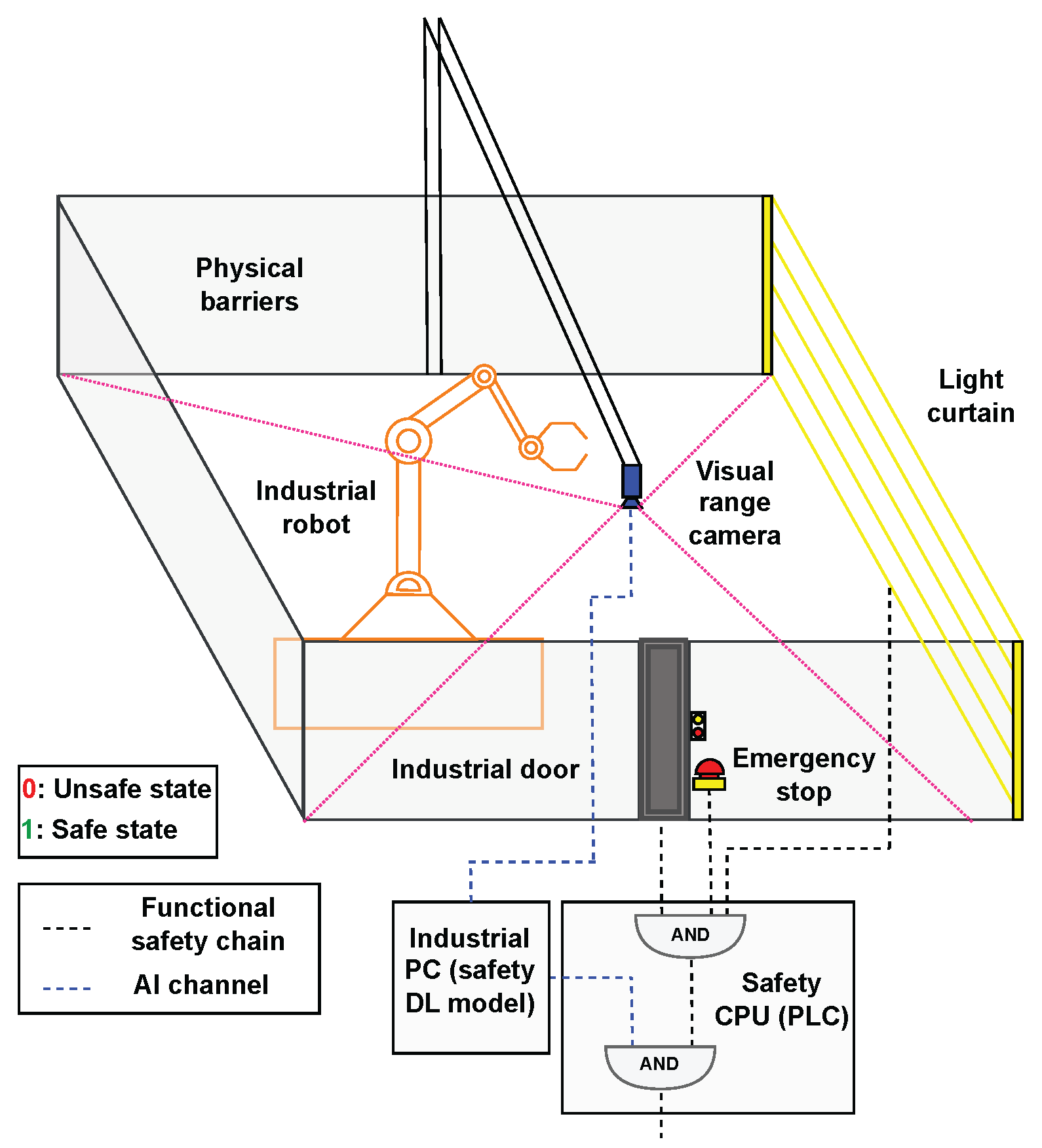
Figure 1. Abstraction of the proposed deep learning-based channel that enhances the functional safety system of an industrial cell. Digital output from the classic safety devices is combined using an AND operation, meaning that, if the safety circuit is interrupted in any device, the machine is switched to a safe state. Similarly, the AI system signal can only alter the previous signal when detecting illegitimate situations that have not broken the safety circuit.
Automation 06 00084 g001
Figure 2. Industrial assembly line used in this work. Several contiguously located manufacturing cells can be seen in (a), while the area of interest to be inspected in each of the cells (delimited by a red dashed line) can be appreciated in (b).
Automation 06 00084 g002
Figure 3. Region of interest to perform the safety inspection. Black peripheral regions correspond to masked areas. Annotated in red are the different industrial components that characterize the facility. This image was captured with the zenithal camera used by our system.
Automation 06 00084 g003
Figure 4. Different categories collected in the dataset. For each image, the bounding box highlights the object responsible for the unsafe situation in the manufacturing cell. Color coding represents the safe (green), unsafe (red), or potentially unsafe (yellow) status of the facility.
Automation 06 00084 g004
Figure 5. Representation of the dataset in an R 2 embedding computed with PaCMAP. Each category is displayed in a different color.
Automation 06 00084 g005
Figure 6. Person and object density distribution by location. The whitish areas indicate the central points of the elements of interest. Contour curves encompass, at different percentiles, the areas with the highest density.
Automation 06 00084 g006
Figure 7. Diagram of the proposed CL architecture. Pairs of images are fed into a siamese network, which extracts their underlying characteristics and projects them into an R 2 latent space. Pairs are projected into nearby or distant regions depending on whether they belong to the same class (two positive images) or not (positive and negative images). Both positive (green boxed) and negative (red boxed) images are processed by a data augmentation module before being fed to the network.
Automation 06 00084 g007
Figure 8. Diagram showing, sequentially, the different phases of the proposed methodology, from data capture to solution deployment.
Automation 06 00084 g008
Figure 9. R 2 latent-space distributions obtained by the different contrastive architectures (Ok vs. Ko). For each distribution, the projections of the supplementary train and test dataset images are represented.
Automation 06 00084 g009
Figure 10. Euclidean distances of the test set latent-space representations to their nearest neighbor in the supplementary training dataset.
Automation 06 00084 g010
Figure 11. R 2 latent-space distributions obtained for the unknown scenarios using the best-performing model (ResNet-18 encoder). Each plot represents the projections of the scenarios with a different type of anomalous object, as well as the supplementary train and the Ok and Ko test scenarios. The blue ellipse represents the BGMM fit to the supplementary train observations.
Automation 06 00084 g011
Figure 12. P–R curves, along with the AUCs, for the best-performing model (ResNet-18 encoder) on the test set. The first category (Ko) represents the test set unsafe scenarios due to the presence of a person. The seven remaining categories collect the potentially unsafe scenarios due to the presence of anomalous objects of different nature.
Automation 06 00084 g012
Figure 13. Pipeline of the proposed patch-based input feature ablations. First, in the pair-matching stage, a safe scenario as similar as possible to the target scenario (unsafe typically; human presence in this case) is sought. Subsequently, small patches of the target scenario are replaced by the equivalent patches of the safe counterpart, computing the deviations produced in the latent space. Finally, a heatmap is built with these deviations, showing which areas of the cell have the greatest influence in being far from the safe representation cluster. The larger the number of patches into which the image is divided ( 2 × 2 , 4 × 4 , …), the more detailed the information about which regions contain information relevant to the prediction. Stronger yellow tones represent patches with greater influence on the latent-space representation calculated by the model.
Automation 06 00084 g013
Figure 14. Graphical user interface screenshots showing the methodology integration in a full-stack software. The underlying industrial configuration is different for confidentiality reasons.
Automation 06 00084 g014
Table 1. Name, number of observations, and cell safety risk for each of the dataset categories. The third column indicates the severity of the scenarios contained in the corresponding category, where ✓ indicates safety, ✗ indicates the presence of a person (maximum risk), and ? indicates the presence of a strange object that may endanger the industrial process.
CategoryNº of ImagesSafety Risk
Ok2912
Ko (Person)3224
Black chair104?
Box263?
Brush180?
Drill14?
Stairs17?
White chair85?
Wire36?
Table 2. Number of images, and their category, for each of the four subsets into which the dataset is split.
DatasetOkKo (Person)Other Objects
Train20742296
Validation484766
Supplementary train208
Test146162699
Table 3. Mann–Whitney U test p-value ( T 1 ) and Pastore and Calcagnì overlapping index ( T 2 ) for the Ok and Ko test set distances displayed in Figure 10.
TestResNet-18DenseNet-161DenseNet-201EfficientNet-B0ConvNeXt-nanoXCiT-nano
T 1 7.24 × 10 52 7.24 × 10 52 7.24 × 10 52 7.24 × 10 52 7.24 × 10 52 7.24 × 10 52
T 2 2.18 × 10 8 2.62 × 10 5 2.53 × 10 14 1.84 × 10 16 8.44 × 10 11 6.07 × 10 6
Table 4. AUCs on the test set obtained by the methodology composed of the different encoders and the BGMM. The first column shows the results for the Ko scenes. The next seven columns show the results for the seven anomalous objects included within the Other objects category. Last column shows the mean AUC for each encoder.
Model AUC Ko AUC Black chair AUC Box AUC Brush AUC Drill AUC Stairs AUC White chair AUC Wire AUC Mean
ResNet-181.00001.00001.00000.99830.96261.00001.00000.98090.9928
DenseNet-1611.00001.00000.99990.71920.92690.90941.00000.98240.9422
DenseNet-2011.00001.00000.99990.99890.93221.00001.00000.97320.9880
EfficientNet-B01.00001.00000.99910.88050.38520.89550.99830.82430.8729
ConvNeXt-nano1.00001.00000.99890.85840.66390.77031.00000.85390.8932
XCiT-nano1.00000.99921.00000.67250.88560.86821.00000.95440.9225
Table 5. AUCs obtained by the hybrid latent-space proposal on the test set. Each subgroup of three rows shows the two base contrastive schemes and the hybrid model resulting from their combination. Columns are the same as in Table 4. A bold font and an asterisk indicate whether the hybrid model improves or worsens the results of the best of its base models for each category.
Model AUC Ko AUC Black chair AUC Box AUC Brush AUC Drill AUC Stairs AUC White chair AUC Wire AUC Mean
ResNet-181.00001.00001.00000.99830.96261.00001.00000.98090.9928
DenseNet-2011.00001.00000.99990.99890.93221.00001.00000.97320.9880
Hybrid model1.00001.00001.00001.00001.00001.00001.00000.98740.9984
ResNet-181.00001.00001.00000.99830.96261.00001.00000.98090.9928
DenseNet-1611.00001.00000.99990.71920.92690.90941.00000.98240.9422
Hybrid model1.00001.00001.00000.99991.00001.00001.00000.98500.9981
ResNet-181.00001.00001.00000.99830.96261.00001.00000.98090.9928
ConvNeXt-nano1.00001.00000.99890.85840.66390.77031.00000.85390.8932
Hybrid model1.00001.00001.00000.99990.98981.00001.00000.9729 ✱0.9953
DenseNet-2011.00001.00000.99990.99890.93221.00001.00000.97320.9880
DenseNet-1611.00001.00000.99990.71920.92690.90941.00000.98240.9422
Hybrid model1.00001.00001.00000.99960.94491.00001.00000.97660.9901
XCiT-nano1.00000.99921.00000.67250.88560.86821.00000.95440.9225
EfficientNet-B01.00001.00000.99910.88050.38520.89550.99830.82430.8729
Hybrid model1.00001.00001.00000.88690.88820.96801.00000.97600.9649
XCiT-nano1.00000.99921.00000.67250.88560.86821.00000.95440.9225
ConvNeXt-nano1.00001.00000.99890.85840.66390.77031.00000.85390.8932
Hybrid model1.00001.00001.00000.8352 ✱0.90240.94271.00000.97030.9563
ConvNeXt-nano1.00001.00000.99890.85840.66390.77031.00000.85390.8932
EfficientNet-B01.00001.00000.99910.88050.38520.89550.99830.82430.8729
Hybrid model1.00001.00000.99980.92530.69570.89931.00000.90320.9279
Disclaimer/Publisher’s Note: The statements, opinions and data contained in all publications are solely those of the individual author(s) and contributor(s) and not of MDPI and/or the editor(s). MDPI and/or the editor(s) disclaim responsibility for any injury to people or property resulting from any ideas, methods, instructions or products referred to in the content.