Abstract
With the advent of the Industry 4.0 era, the manufacturing industry is implementing a range of novel technologies on the factory floor, leading to the generation of substantial quantities of production data. However, the development of analytics tools capable of processing these data and extracting valuable information for decision-making and production control lags behind. In addition, a noticeable amount of raw data collected from the factory floor is prone to errors, especially in small- and medium-sized manufacturing plants, and their processing often requires a laborious data cleaning process due to the limitations of the sensors and the noisy environment of the manufacturing facilities. This presents a challenge in utilizing factory floor production data effectively. This paper addresses the challenge by focusing on the parts flow data, which reflects the number of parts in each buffer as a function of time in a production system. In particular, we study the parts flow data in discrete-time serial production line models, assuming that the data are subject to random noise, and develop effective and robust algorithms that can effectively detect and correct errors in these data. To improve the computational efficiency for complex cases (longer lines, higher error rates, etc.), a decomposition-based approach is used to parallelize the computation procedure at implementation. Numerical experiments demonstrate that the proposed methods can enhance data quality by more than 40% and improve the accuracy of system performance metrics estimation by over 50% using corrected data. These improvements can facilitate more reliable process monitoring and production control in manufacturing environments.
1. Introduction
Industry 4.0, also known as the fourth industrial revolution, marks a major shift in the manufacturing area, where digital technologies are integrated into industrial processes, facilitated by the widespread connectivity of the Internet. The concept of Industry 4.0 was initially introduced by the German government in 2011 [1], with the objective of leading the development of “smart factories” that utilize the power of interconnected cyber-physical systems. At the core of the Industry 4.0 paradigm is the convergence of cutting-edge technologies, which include networked physical systems, Internet of Things (IoT) devices, cloud computing infrastructure, artificial intelligence (AI), and advanced data analytics [2]. This integration revolutionizes manufacturing operations, enabling unprecedented levels of real-time data collection, analysis, and decision-making. Within the Industry 4.0 framework, Smart Manufacturing emerges as a manufacturing regime for the foreseeable future, powered by the development of sophisticated automation and control systems [3]. These systems enable factories to operate autonomously, adapt to changing conditions, and continuously optimize performance. By utilizing sensors and connection technologies, smart factories can accumulate comprehensive time series datasets that encompass a wide range of factors, such as the status of equipment, manufacturing processes, and metrics related to product quality along with time. Such time series data holds immense potential to improve product quality, increase efficiency, and simplify supply chain management, as discussed by [4].
While high accuracy sensing and automated data-collection mechanisms are commonly deployed in the infrastructure of modern, large manufacturing plants (e.g., in automotive, semiconductor industries), numerous small and medium-sized manufacturers (SMMs) lag behind in adopting new technologies in their production practice due to space, personnel, and cost challenges. In SMM plants, even when good quality sensors would be deployed, aging equipment, limited floor space, retrofitted sensor installations, and suboptimal layouts may frequently lead to erroneous data. Additionally, due to cost constraints, sensors used in these manufacturers are often of low-resolution or lack redundancy, making them more susceptible to errors caused by environmental factors such as vibration or lighting changes. Indeed, while vast amount of production systems research results have seen applications in real manufacturing practices, most were targeted as large-scale mass manufacturing systems. For the limited number of applications reported at SMMs, they typically required dedicated personnel to manually perform on-site time studies for extended period. Moreover, such studies require recording uptime and downtime of each production operation. This may be challenging and highly case-dependent in production systems of SMMs, which often involve a great portion of manual labor in the production process. We started addressing this issue by proposing to only use parts flow data (buffer occupancy) to accomplish the identification of the mathematical model parameters for a production system (see [5,6,7] for more details) due to the fact that part counting is much more straightforward and easier to standardize (than defining uptime and downtime for various kinds of production operations in different manufacturing applications). We view this as a path to enable easier construction of production system mathematical models for SMMs and to facilitate adoption of more advanced techniques of system optimization and control. The current paper is intended to address the potential data quality issues that the above-mentioned parts flow data-based production system modeling approach may encounter, especially in systems of SMMs. Specifically, rather than simply assuming that the manufacturers can easily replace/upgrade sensors, we aim to maximize the utility of data, which are collected in a potentially non-ideal environment or by non-ideal devices, by identifying and correcting errors algorithmically, thereby enabling higher data accuracy for subsequent analysis and decision-making. Our approach complements sensor-level improvements and offers a cost-effective and scalable alternative, particularly suited to the needs of small and medium-sized manufacturers.
Parts flow data, a key form of time series data on the factory floor, plays a vital role in monitoring, controlling, and optimizing manufacturing systems. However, this data is often affected by measurement errors caused by sensor limitations and environmental changes. The reliable detection and correction of these errors are critical to ensuring accurate system behavior and supporting data-driven decision-making. Despite its significance, this topic remains relatively underexplored in current research. At the system level, Jin et al. proposed a data fusion method for quality-related sensor data using a principal component regression model to correct systematic biases in multivariate parts flow records, and Mhada et al. also contributed valuable insights by examining how unreliable inspections can misrepresent part positions and movements, ultimately distorting flow information (for comprehensive reviews, see [8,9]). Complementing these efforts, Ref. [10] provided a comprehensive review of statistical process monitoring in the presence of measurement errors, highlighting how such errors can distort control charts and lead to false alarms. Based on this, Ref. [11] introduced an enhanced p-control chart that incorporates error correction mechanisms for small-sample datasets affected by false records or misclassification. Their approach modifies the exponentially weighted moving average (EWMA) method to adaptively adjust control limits, thereby enhancing robustness against sensor-induced errors. In addition to control chart enhancements, various statistical and model-based techniques have been employed to address errors in parts flow data. Kalman filtering and moving average smoothing are frequently used to mitigate high-frequency fluctuations, while rule-based approaches flag errors based on physical constraints, such as negative inventory or buffer capacity exceeding. More recent developments include predictive noise correction pipelines, such as the framework proposed by [12], which identifies invalid or missing readings and imputes likely values using feature selection and a Random Forest model. Similarly, Ref. [13] identified common error types, such as stuck-at-zero, bias, and outliers, and recommend advanced strategies like autoencoder-based error detection and hybrid data fusion to improve data reliability in complex manufacturing environments.
The literature review indicates that few studies have focused on error detection and correction specifically for discrete parts flow data in manufacturing systems, where operational constraints define nonlinear relationships between variables. Moreover, traditional methods such as Kalman filtering or smoothing are designed for continuous-valued data and are not directly applicable to integer-valued, constraint-driven production flows. This gap highlights the lack of algorithms that leverage operational constraints in discrete time-series data. To address it, we develop computational algorithms to detect and correct errors for serial production lines. The proposed methods are validated through numerical simulations, demonstrating their effectiveness in enhancing the accuracy and reliability of production system monitoring and analysis.
To evaluate performance, we use both Bernoulli and geometric reliability models to generate parts flow data and apply several noise models to simulate realistic measurement errors observed in small and medium-sized factories. The proposed algorithms are tested on both two-workstation and multi-workstation lines, with performance evaluated by improvements in the estimation accuracy of system metrics (production rate and work-in-process).
The main contributions of this paper are as follows:
- We propose error detection criteria to flag suspicious part flow data entries that may potentially contain errors. For two-workstation lines, we develop a data-block-based correction approach that involves constructing data blocks and enumerating valid combinations under data integrity constraints to minimize required modifications. For multi-workstation lines, we introduce a two-stage decomposition-and-aggregation-based correction method to manage the increased complexity effectively.
- Our error detection and correction framework offers a practical solution to reliable utilization of parts flow sensor data in small and medium-sized manufacturing environments without requiring high-precision sensor setup or costly data fusion technologies. The computational load is lightweight and can be handled by affordable computing resources.
- From a practical perspective, the proposed method supports intuitive and accessible modeling of part flow data. It simplifies error analysis and correction, making it usable by practitioners without deep theoretical or statistical expertise.
The remainder of the paper is structured as follows: Section 2 introduces the serial production line model, defines notations, and formulates the problems addressed in the paper. Section 3, Section 4.1 and Section 4.2 present the proposed methods for error detection and correction in parts flow data for two- and multi-workstation serial lines, respectively, along with their computational implementation and numerical experiments to assess their performance. Finally, Section 6 summarizes the conclusions and highlights potential future work.
2. Problem Formulation
2.1. Model Assumptions
Consider a serial production line consisting of M workstations, either automated or operated manually, interconnected by intermediate buffers, as illustrated in Figure 1. The notation used in this section is summarized in Table 1. Each buffer is equipped with a sensor that continuously records the number of parts present, producing a time series of parts flow data. These sensors are used solely for data acquisition and do not influence production decisions such as starvation or blockage events. As noted in [5,6,7], such data can provide valuable insights for estimating the parameters of mathematical production system models. In practice, parts flow monitoring can be implemented using a variety of sensing modalities, including photoelectric sensors, weight sensors, camera sensors, etc. However, due to technical limitations of the sensors and noise in an SMM environment, the recorded measurements frequently exhibit inaccuracies or noise, making the true system state only partially observable. Consequently, the collected data must be preprocessed to remove inconsistencies, correct erroneous values, and enhance overall data quality for subsequent analysis.
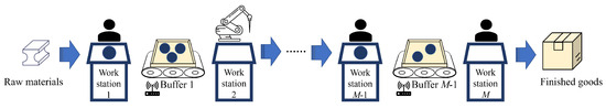
Figure 1.
Serial production line with M workstations.

Table 1.
Glossary of symbols used in the model.
To formally model system operations, we assume the following:
- All workstations operate with a common cycle time , and the system is viewed in discrete time with slot length .
- Buffer i can store up to parts.
- Workstations may experience random, unscheduled downtime.
- Workstation i becomes starved if it is up during a time slot but Buffer is empty at the beginning of the time slot. Workstation 1 is always supplied with raw material.
- Workstation i becomes blocked if it is up during a time slot but Buffer i is already full and Workstation is unavailable. Workstation M never becomes blocked by downstream inventory.
- When operational and neither blocked nor starved, a workstation processes one part from its upstream buffer (or raw material source for Workstation 1) and deposits the processed part into its downstream buffer (or finished goods storage for Workstation M) at the end of the time slot.
Remarks: Serial production lines of this type have been extensively investigated in the production systems literature (e.g., [14,15,16,17]). In this study, we use both Bernoulli [18] and geometric [19] reliability models to generate synthetic parts flow data for numerical experiments. These two reliability models reflect different operational characteristics: Bernoulli reliability is well suited for assembly-type systems where workstation downtime are short relative to the cycle time, whereas geometric reliability is more appropriate for operations where downtime are significantly longer. The resulting simulated data serve as the basis for developing and testing the error detection and correction algorithms proposed in this paper. Extensions to continuous-time models and other system structures, such as assembly lines, will be pursued in future research.
2.2. System State Evolution and Performance Metrics Calculation
A serial production line with multi-workstations, defined by assumptions (1)–(6), can be described as a discrete-time stochastic process. Based on the system model assumptions, the parts flow of a buffer may change at the beginning or at the end of a time slot. Specifically, at the beginning of a time slot, the downstream workstation may remove a part from a (non-empty) buffer if the workstation is up and not blocked. At the end of a time slot, the upstream workstation may release a new part into its outgoing buffer if the workstation is up and not starved. Therefore, when evaluating the work-in-process or the parts flow of a buffer, two measurements are possible depending on the timing:
- : the number of parts in Buffer i during time slot n, i.e., after the workstations have picked up parts from upstream buffers (or raw material supply) and started processing them.
- : the number of parts in Buffer i at the end of time slot n, i.e., after the workstations have completed processing parts and routed them to the downstream buffers (or finished goods inventory).
Let denote the number of parts processed by Workstation i during time slot n. Then, we obtain Equations (1)–(3).
In the analysis of production systems, two performance indicators are of central interest: the production rate (), or throughput, and the work-in-process (). These quantities provide a quantitative summary of how effectively material flows through the line and how much inventory accumulates within the buffers. When observing the system over a time horizon of length T, the long-run average production rate can be expressed as the mean number of completed parts released by Workstation M. Using the buffer-level dynamics derived earlier, this quantity is computed as Equation (4).
Similarly, the average work-in-process of Buffer i over the observation horizon T is given by Equation (5).
2.3. Problem Addressed
In this paper, we assume that sensors are installed throughout the system to monitor the parts flow. Specifically, each buffer occupancy sensor records the parts flow data both during a cycle time (to measure ) and at the end of a cycle time (to measure ). Let and denote the measured parts flow by the sensors. This leads to a table (matrix) of the measured data in Equation (6).
Based on the measured parts flow data, the corresponding system performance metrics can be estimated using Equations (7) and (8).
Note that it is possible to show that measuring just the data during system operations is not sufficient to determine ’s. In other words, parts flow measurements of buffers still must be taken. In this paper, we assume that workstation production data ’s are not directly measured and only parts flow in the buffers, ’s and ’s, are measured, which can be further used to infer ’s based on Equations (1)–(3). It should also be noted that collecting more data usually leads to higher redundancy, which, in turn, can help the process of cleaning the raw data and improving the data quality. However, this also increases the cost of implementation and the complexity of the data cleaning process. In future work, we will study the cases, where multiple types of sensor data are used for performance monitoring and model parameter identification.
As discussed above, measurements obtained from sensors in SMM production environments are often unreliable because of device limitations and the presence of substantial noise. Consequently, the recorded values may not accurately reflect the true parts flow. Before such data can be used for analysis, a preprocessing stage is typically required to enhance data quality, which involves detecting and correcting erroneous or inconsistent entries. To assess how these measurement errors influence the estimation of parts flow-related performance metrics, we examine several noise models.
- Noise Model 1In this noise model, each measurement differs from the true parts flow value with probability q. When an error occurs, the sensor outputs a value selected uniformly at random from the feasible set that is not equal to the true value. The corresponding theoretical formulations are provided in Equations (9)–(11).
- Noise Model 2In the second noise model, the measured buffer occupancy is different from the true data, again, with probability q. However, in the event of an error, the sensor may produce a random value from the feasible range following a triangle distribution, whose functions are given in Equations (12) and (13). Figure 2 illustrates an example of the probability distribution defined by Noise Model 2.
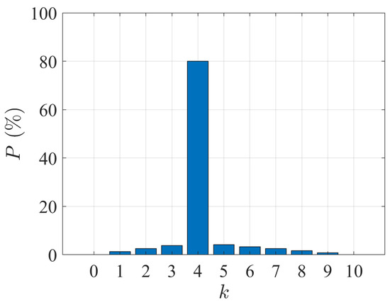 Figure 2. Example of probability distribution of under Noise Model 2 ().
These error models represent some typical situations in practice, where the measurement is susceptible to environmental noise, such as variable lighting conditions that may affect a camera sensor. Additionally, these models can be applied when the precise nature of the error is unknown. Additional experiments with three alternative noise models are provided in Appendix A.
It is clear that errrors in the raw data can directly affect the estimated performance metrics, as reflected in the measured performance metrics given in Equations (7) and (8). These inaccuracies could potentially undermine the effectiveness of production control and decision-making processes, ultimately leading to reduced system efficiency. In this paper, we address these issues arising from the production system model described by assumptions (1)–(6) and the parts flow measurement model outlined in Equations (9)–(13). Specifically, we aim to tackle the following problems:
- Data error detection: Given the parts flow measurement dataset , determine if erroneous entries are present in the data (i.e., if there exist n and i such that or );
- Data error correction: Identify the locations of the errors in the parts flow measurement data and correct them to obtain the corrected dataset , where
3. Two-Workstation Case
As mentioned above, for the case of two-workstation serial lines, preliminary results on the criteria and algorithms for error detection, identification, and correction have been developed in our prior work [20]. To keep the current paper self-contained and since the two-workstation line results are the foundation for the multi-workstation line case to be discussed in Section 4.1 and Section 4.2, here we provide an overview of the key results from [20].
- Two-workstation Error Detection Criteria (TEDC) [20]:
- If , then an error exists in or or both.
- If , then an error exists in or or both.
Note that TEDC presents a sufficient condition of the existence of data errors but not necessary. In other words, some errors may not be identified by these criteria, and the criteria alone are insufficient to determine which specific data entry is erroneous.
To identify and correct errors in the parts flow data, we observe that the measured dataset can be organized as a table in which each row n corresponds to the measurements collected at time slot n (see Figure 3 for an illustration). Note that, however, since this table may vary in sizes, it could be computationally challenging or even intractable to perform data correction on the entire table directly. Therefore, we propose an approach to decompose the entire data table into a number of data blocks and perform data correction within each individual block separately. This may reduce the computational burden and also enable parallel computing to accelerate the solution process. In this dataset, we define a data block , denoted , as the collection of rows between indices and . Here, and serve as the starting and ending boundary rows, marking the portion of the data in which errors are suspected while providing reliable reference points on both sides. These boundary rows are identified using the criteria specified in Equations (14) and (15).
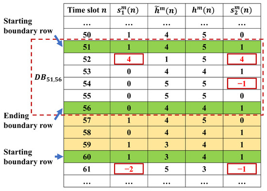
Figure 3.
Illustration of data block construction with boundary rows.
As one can see, these conditions are set based on the presence of consistent binary values in the inferred parts flow data (on the machines), which indicate error-free behavior. The starting boundary row is located just before the data begins to deviate from this binary pattern, while the ending boundary row is placed where the data returns to a consistent binary state. In the computational implementation, the data table is scanned row-by-row, from the beginning, for Equation (14). Once it is met, the row being inspected is marked as the starting boundary row of a new data block. Next, the subsequent rows are scanned for Equation (15). Once this condition is met, it is marked as the ending boundary row of the current data block and the algorithm returns to the scan for the starting boundary row of the next data block. This process is repeated until all rows of the data table are scanned. The starting and ending boundary rows, thus identified, will result in a number of data blocks covering different portions of the entire dataset.
This approach ensures that each data block targeted for correction is bounded by trustworthy data, enabling more accurate estimation and reducing computational burden by limiting the correction scope to localized regions rather than the entire dataset. It is worth noting that Equations (14) and (15) imply that some rows may not be included in any of the constructed data blocks when they contain no entries flagged as questionable by TEDC.
To illustrate the construction of a data block, consider the section of parts flow and workstation production data shown in Figure 3. In this example, rows 51 and 56 conform with the definitions of starting boundary rows and ending boundary rows, thus, forming a data block denoted as . Notably, TEDC flags , , and as erroneous data since they fall outside the feasible set of {0,1}. It then follows from TEDC, error may be present in , , , , and/or . As a result, other ’s and ’s in this data block may be also subject to errors contained in the questionable parts flow data and will be involved in the data correction process to be described next.
Moving from row 56 down to row 61, the workstation production data ’s and ’s all fall within their feasible set {0,1}. Then, this is violated in row 61, where and , which makes its previous row, row 60, the starting boundary row of a new data block. Scanning each row of the data table and continuing this procedure will result in a number of data blocks that cover all questionable data entries marked by TEDC.
It should be noted that the data block construction and subsequent error correction process rely solely on the binary processing status of the workstation (i.e., whether it processed a part or not), which remains consistent regardless of the workstation reliability model, Bernoulli, geometric, or otherwise. While the choice of reliability model affects the generation of parts flow data and consequently influences the frequency and distribution of binary values (0 s and 1 s) in the deduced production status, our method is designed to operate independent of the underlying reliability models of the workstations and based only on the inferred binary characteristics of workstation activity.
Based on the data blocks, the Two-workstation Error Correction Algorithm (TECA) for parts flow data in two-workstation serial lines is summarized in the pseudo-code in our prior work [20].
4. Multi-Workstation Case
4.1. Error Detection Criteria
In this section, we extend the error detection criteria of two-workstation lines (TEDC) to multi-workstation cases (MEDC).
For multi-workstation lines, the workstation production status of each time slot can be estimated based on the parts flow data similar to the two-workstation case. Specifically, for Workstation 1 and Workstation M, the expressions in Equations (1) and (3) take the measurement-based forms shown in Equations (16) and (17).
For internal workstations, , , since each of them is connected with two buffers, we can estimate its production status from either its upstream buffer, denoted as , or its downstream buffer, denoted as in Equations (18) and (19).
To detect potential errors in the data, we first confirm whether the deduced values of , , comply with the system constraints. If they do not, error detection criteria are designed.
- Multi-workstation Error Detection Criteria (MEDC):
- If , then error is potentially present in or or both.
- If or or , then error is potentially present in , , , and or a subset of them.
- If , then error is potentially present in or or both.
Similar to TEDC in the two-workstation case, MEDC can be used to identify suspicious parts flow data entries that may potentially contain errors.
4.2. Error Correction Process
MEDC encounters the challenge of accurately identifying data entries that actually contain errors. In addition, an exhaustive search for all potential error correction options throughout the entire dataset would be excessively complex and time-consuming. Therefore, for systems with multiple workstations and buffers, we propose a decomposition/aggregation-based approach to overcome these challenges. The steps of this method are illustrated in the flow chart of Figure 4. Each of them is outlined below.
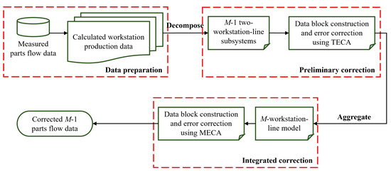
Figure 4.
Decomposition/aggregation-based data correction method for M-workstation serial lines.
- Data preparation
- Preliminary correctionIn this step of the error correction process, we decompose the M-workstation line into two-workstation-line subsystems. This is illustrated in Figure 5. For each resulting two-workstation line, a sub-dataset is constructed that contains the parts flow data from the buffer belonging to this subsystem, and the workstation production data is calculated based on this buffer’s parts flow data. Specifically, for the two-workstation-line subsystem with Workstation 1, Workstation 2 and Buffer 1, the sub-dataset consists of entries of , , , and ; for the two-workstation-line subsystem with Workstation i, Workstation and Buffer i, , the sub-dataset consists of entries of , , , and ; for the two-workstation-line subsystem with Workstation , Workstation M and Buffer , the sub-dataset consists of entries of , , , and .
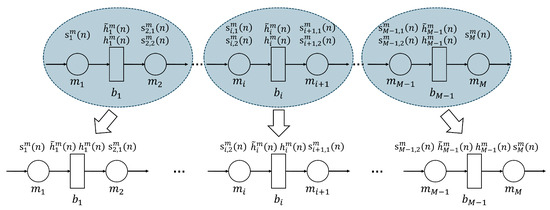 Figure 5. Decomposition of M-workstation line into two-workstation-line subsystems.
With the above decomposition, we treat each two-workstation-line subsystem independently in this step and apply TECA to each sub-dataset constructed above. Note that preliminary correction is intended to identify and correct the errors in the parts flow data entries locally, i.e., within each two-workstation-line subsystem.
Upon completion of the preliminary correction, the workstation production data, , , , and , are guaranteed to be within their feasible range of . However, since the corrections are performed locally and for given i, and belong to the datasets of different subsystems, inconsistency between them may still exist after preliminary correction. This potential problem will be addressed in the next step, integrated correction.
- Integrated correctionIn this step, we aggregate the two-workstation-line subsystems from the preliminary correction back into the original M-workstation serial line structure. An integrated dataset for the whole M-workstation-line system is constructed by merging the TECA-corrected sub-datasets from preliminary correction. An illustration is given in Figure 6 for an -workstation line case. In this illustration, the data of and are obtained from subsystems -- and -- from the previous step, as shown in Figure 6.
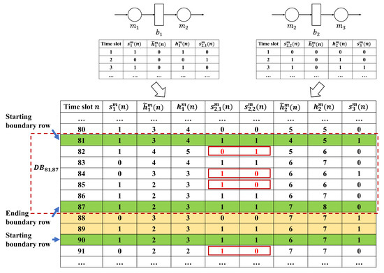 Figure 6. Illustration of dataset merging and boundary row identification for integrated correction.
Now, to identify and correct the errors in the merged dataset comprised of multiple workstations and multiple buffers, the data-block-based method described in Section 3 is extended to the Multi-workstation Error Correction Algorithm (MECA). In this case, the data table is partitioned into blocks using the starting and ending boundary rows specified based on MEDC. Specifically, if the data entries in two consecutive rows and satisfy the consistency constraint (20).
for all , and the entries in the subsequent row fails to meet the above constraint for at least one , then row is designated as the starting boundary row of a data block. Then, starting from row and scanning the data in each row that follows , if the data entries in row do not satisfy consistency constraint (20) for at least one , but the entries in the subsequent two consecutive rows and do for all , then row is identified as the ending boundary row of this data block.
To illustrate the construction of a data block, consider again the parts flow and workstation production data after the preliminary correction, as depicted in Figure 6. In this example, row 81 is first identified as the starting boundary row of a data block since the data entries in rows 80 and 81 all pass constraint (20) but row 82 has entries violating (20) (). The next several rows either have entries violating constraint (20) (rows 82, 84, 85) or are immediately followed by a row with data violating (20) (row 83 passes MEDC but row 84 fails), until rows 86 and 87, where (20) is met for two consecutive rows, which makes row 87 the ending boundary of this data block. The data blocks, thus obtained, should encompass a great portion of the data set but does not necessarily cover the entire dataset. For the example shown in Figure 6, rows 88 and 89 do not belong to any data blocks.
With the data blocks constructed, the identification and correction of erroneous data entries will be performed within each individual data block. Note that it follows from Equations (1)–(3) that the parts flow and workstation production data variables of an M-workstation serial line satisfy Equations (21) and (22).
The measured data should follow the same relationships. Thus, for a given data block with starting boundary row and ending boundary row , the above Equations (21) and (22) can be rewritten as Equations (23) and (24).
Using Equations (23) and (24), one can trial different combinations of workstation production data, ’s, calculate the corresponding parts flow data, and , and determine the combinations of workstation production data that are most likely to represent the true data. However, due to a greater amount of data entries in the multi-workstation case, it is computationally infeasible to replicate the TECA approach and enumerate all valid combinations of workstation production data. Therefore, a procedure is developed to only inspect a select set of the most suspicious combinations of workstation production status to ensure a manageable computing burden. Specifically, for the data block with starting and ending boundary rows and , let denote the set of workstation production data within the data block that will be trialed in Equations (23) and (24). Then,
- For Workstation i, , is selected into if
- –
- , or
- –
- but ;
- For Workstation 1, is selected into if is selected into ;
- For Workstation M, is selected into if is selected into .
Following this procedure, the data entries not selected into are assumed to be error-free and will remain unchanged during the data correction process. As a result, a total of combinations of workstation production status will be tested (with each data entry taking a value of either 0 or 1) to identify potential erroneous data entries, as opposed to combinations if all workstation production data were to be enumerated. For each of the combinations examined, Equations (23) and (24) are used to calculate the corresponding parts flow data and . If the resulting and are within their feasible ranges , then the algorithm proceeds to calculate the number of data entries modified compared with the original measured parts flow data. The combination with the minimal number of modified entries is output as the final corrected dataset.
Figure 7 shows an example of the above data entry selection procedure for a five-workstation line. In this example, for the data block bounded by row 35 and row 40, inconsistency is observed between and , and , and , and , and and , which are indicated by the red boxes in the figure. They lead to , , , , and to be selected into for calculation in Equations (23) and (24). Then, , and are also selected into since , and are selected due to inconsistency observed (indicated by purple arrows). Finally, , , , , , and are selected into since , , , , , and have all been selected (indicated by orange arrows). The resulting consists of 14 workstation production data entries out of the 20 total in the data block—reducing the computation burden for this data block to only 1.56% of the total enumeration approach. The entire process of MECA for integrated correction is provided as a pseudo-code of Algorithm 1.
| Algorithm 1: Multi-workstation Error Correction Algorithm (MECA) |
 |
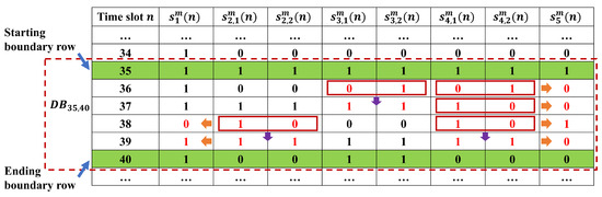
Figure 7.
Illustration of selecting data entries in a data block to be examined during integrated correction.
5. Numerical Experiments
5.1. Error Detection
To justify the performance of the error detection criteria, TEDC and MEDC, a simulation study is carried out. Specifically, we generated 1000 serial lines with workstations following the Bernoulli reliability model and another 1000 serial lines with workstations following the geometric reliability model for time slots. For the Bernoulli lines, the workstation efficiency ’s are randomly and uniformly selected from and the buffer capacity ’s are randomly selected from . For the geometric lines, the workstation efficiency ’s and repair probabilities ’s are randomly and uniformly selected from and , respectively, while the buffer capacity ’s are randomly selected from .
To quantify the performance of TEDC/MEDC, we employ the performance metrics True Positive Rate (), False Positive Rate (), and Accuracy (), commonly used in binary classification, given in Equations (25)–(27).
where (true positive) and (false negative) represent the number of actual erroneous entries marked by TEDC/MEDC and the number of undetected erroneous entries, respectively. (false positive) and (true negative) denote the number of actual true entries falsely marked by TEDC/MEDC and the number of actual true entries remaining. is the total number of data entries. These metrics are calculated based on the numerical experiment results and their average values are summarized in Table 2 and Table 3.
Table 2.
Performances of data error detection (Noise Model 1).
Table 3.
Performances of data error detection (Noise Model 2).
These results also provide insight into the sensitivity of the error detection criteria with respect to q and M. As one can see, TEDC and MEDC are intended to be relatively conservative measures. On average, TEDC can detect over 80% of erroneous data entries while maintaining a relatively low (10–30%). In contrast, MEDC achieves a higher detection rate of 96%, but at the cost of a potentially higher (30–50%). The overall accuracy declines as the error rate q increases due to the conservative nature of the criteria, indicating that the criteria are more sensitive to the error rate than to the number of workstations.
To assess the statistical significance of the observed differences in detection performance, a two-way ANOVA is conducted with q and M as factors. The resulting F-statistics, p-values, and partial values are summarized in Table 4 and Table 5 for Noise Models 1 and 2, respectively. The results indicate that both q and M have statistically significant effects on the performance metrics (p-value ), with M showing a dominant influence on all three indicators. The interaction between q and M is also significant, though with smaller partial . The statistical results demonstrate that the observed differences are robust and that the proposed detection criteria maintain stable and reliable performance across various scales and noise levels.
Table 4.
Two-way ANOVA results for the effects of M and q (Noise Model 1).
Table 5.
Two-way ANOVA results for the effects of M and q (Noise Model 2).
5.2. Error Correction
The efficacy of TECA for two-workstation line models is studied in [20], which shows that the noises in the parts flow data may lead to large errors in estimating the system performance metrics and , as large as about 20% on average for estimation when or higher. Then, it was demonstrated that TECA performed effectively in identifying and correcting the errors and, as a result, substantially increased the estimation accuracy (dropping the estimation errors to below 5% for and below 1% for ). It can also substantially reduce the number of erroneous data entries (by about 60–80%). Even for those that are still not consistent with the true data after TECA, the deviation of erroneous data entries from the true ones is at the minimal value 1 in about 95% of cases.
For multi-workstation lines, to investigate the accuracy of the two-stage decomposition aggregation-based parts flow data correction method described above, 500 ten-workstation Bernoulli lines and 500 ten-workstation geometric lines under each noise model are generated for time slots. For the Bernoulli and geometric lines, the workstation and buffer parameters are randomly selected from the same ranges used in the numerical experiments in Section 5.1.
For each line, thus constructed, we calculate its average production rate and work-in-process using Equations (7) and (8). Subsequently, we estimate the relative errors by comparing the measured data before ( and ) and after ( and ) the MECA method is applied, as defined in Equations (28)–(31).
where and are the performance metrics calculated by the corrected parts flow data and here.
As a comparison, we also include another method, referred to as Deletion Method, which directly excludes the potentially erroneous data entries marked by MEDC from the calculation of the system’s performance metrics. In other words, the system performance metrics, denoted as and , are calculated using the remaining data after deletion of the questionable ones. The underlying assumption of this method is that removing erroneous data entries eliminates their negative influence without significantly distorting the overall statistical behavior of the production flow. Although this method is simple and computationally efficient, it may result in information loss and biased estimates when the proportion of deleted data is large. The accuracy of these performance metric estimates is evaluated based on Equations (32) and (33).
The results are summarized in Figure 8 and Figure 9, Table 6 and Table 7. Similar to the two-workstation case, the large estimation errors of and using the raw data under two noise models can be greatly reduced after the correction method is applied. For the geometric line case with , the correction can bring down the average estimation error from almost 30% to just above 6%. For all cases studied, the correction of parts flow data errors can reduce the and estimation errors by over 75% for Noise Model 1 and by over 50% for Noise Model 2. Moreover, the robustness of the results is also improved, shown by the whiskers (95% confidence intervals) in Figure 8 and Figure 9. The Deletion Method not only results in a reduced estimation accuracy for and , its main drawback is the increased data loss with higher values of q. Specifically, the amount of data discarded grows, peaking at 70% when . This underscores the considerable constraints of using this elimination-based strategy, especially in a real-time data processing environment where the data space is relatively small. As shown in Table A1 in Appendix A, the three additional noise models yield similar results.
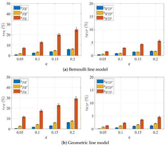
Figure 8.
Errors of and estimation before and after deploying the data correction methods to ten-workstation lines (Noise Model 1).
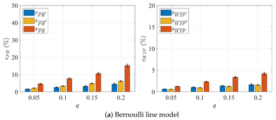
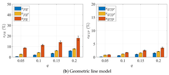
Figure 9.
Errors of and estimation before and after deploying the data correction methods to ten-workstation lines (Noise Model 2).
Table 6.
Average estimation error of performance metrics for ten-workstation lines (Noise Model 1).
Table 7.
Average estimation error of performance metrics for ten-workstation lines (Noise Model 2).
To further illustrate the performance of the MECA method, Figure 10 and Figure 11 show the average fraction of data entries inconsistent with true ones before () and after () correction is applied. Notably, when the error rate q is no greater than 0.1, the method exhibits a substantial reduction in the number of erroneous data entries, ranging from 40% to 70%. As the value of q increases, the extent of reduction becomes less pronounced, stabilizing at approximately 20% to 40%. However, it is essential to highlight, as depicted in Figure 10 and Figure 11, that even in those cases, the discrepancy between the corrected data entries and the true ones is reduced by about 50%, indicating a substantial enhancement in data quality for multi-workstation production lines.
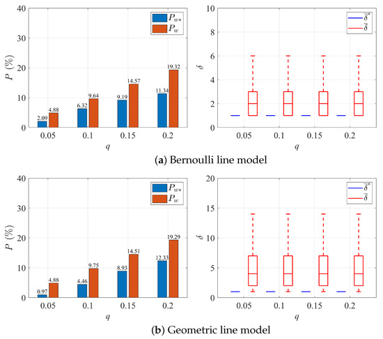
Figure 10.
Error correction performance and average difference before and after deploying our method to ten-workstation lines (Noise Model 1).
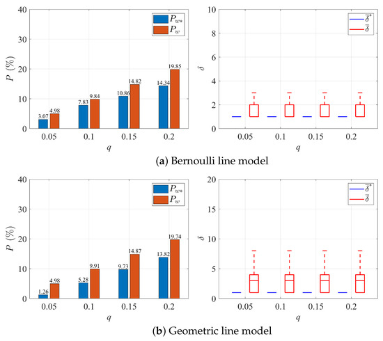
Figure 11.
Error correction performance and average difference before and after deploying our method to ten-workstation lines (Noise Model 2).
In addition, Figure 12 reports the proportion of data discarded by the Deletion Method. As shown, the fraction of data loss increases rapidly with q, reaching more than 70% when , which further demonstrates the advantage of MECA in preserving data and avoiding excessive information loss.
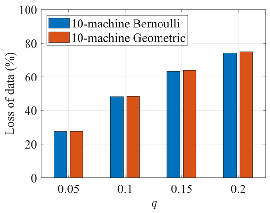
Figure 12.
Discarded data entries for multi-workstation lines by Deletion Method.
In Figure 13, we provide an example to illustrate the efficacy of MECA by viewing a segment of the parts flow time series data, , over 100 time slots, both before and after undergoing correction. As one can see from the figure, the raw data (red line) contains 11 erroneous entries, some of which deviate from the true data (green line) due to measurement noise. Upon applying MECA, the corrected data (blue line) and the true data almost completely overlap, with only 4 erroneous entries remaining, all with minimal deviation. The correction process effectively mitigates large discrepancies, though it inadvertently modifies 2 data entries and fails to detect one erroneous entry. Nonetheless, the overall improvement in data accuracy is substantial.
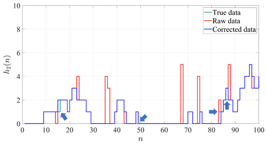
Figure 13.
Example of Bernoulli production line parts flow data before and after correction ().
5.3. Computation Implementation
It should be noted that as the parameter q increases, the dataset tends to generate more erroneous data, leading to a diminishing number of boundary rows. Consequently, there is a growing likelihood of encountering larger-sized data blocks when executing the proposed data correction method, especially for the two-workstation-line subsystems in the preliminary correction stage. The correction process for these larger data blocks may become notably much more time-consuming compared to their smaller counterparts. To optimize computational efficiency, parallel processing is first employed for handling the data blocks in the two-workstation-line subsystems during preliminary correction and the multi-workstation line during integrated correction, as illustrated in Figure 14. Then, during its initial implementation for two-workstation-line subsystems, an increase in computing time was observed for data blocks with 14 rows or larger. Consequently, it is then decided that data blocks of size no greater than 13 rows are treated as parallel tasks. Threads are thus allocated until all available threads are engaged to correct errors in each block simultaneously. For a data block with more than 13 rows, we divide the for-loop within TECA (line 10 to line 28 of Algorithm 1 pseudo code) into L smaller loops, each treated as a thread in parallel with other tasks (such as correction of smaller data blocks). Table 8 presents a summary of the average computing time for two-workstation and ten-workstation production lines under the above parallel implementation strategy. For each value of q, the computing times are evaluated for 100 Bernoulli lines and 100 geometric lines altogether. The algorithms were programmed in C++ and executed on a DELL workstation (Dell Inc., Round Rock, TX, USA) with a 10-core Intel(R) (Intel Corporation, Santa Clara, CA, USA) Xeon(R) E5-2650 CPU 2.30 GHz processor having 20 threads allocated for parallel computing and 32 GB of RAM.
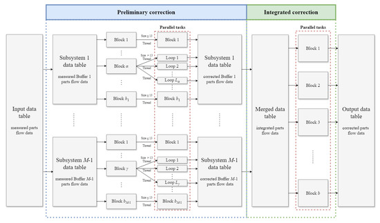
Figure 14.
Parallel computing framework for parts flow data correction in M-workstation serial lines.
Table 8.
Computing time using parallel processing.
Notably, when q is very small, parallel processing has a marginal impact on computing time, requiring only a few seconds or minutes. However, as q increases, the computing time experiences a surge, with instances where it extends to about 4 h for ten-workstation lines when q is 0.2. Figure 15 shows the (average) breakdown of the computing time for this case ( and ) from numerical experiments. Specifically, preliminary correction consumes, on average, 3.29 h (about 82% of total computing time). This amounts to about 21.9 min per two-workstation-line subsystem. Integrated correction consumes, on average, 7.3 min (about 3% of total computing time), and other computation overhead uses about 37.4 min (about 15% of total computing time). If, hypothetically speaking, the algorithm were to be implemented on a 20-core-40-thread CPU with similar ancillary hardware, it is expected that preliminary correction could be finished in about 2.08 h. This translates to a time savings of 1.21 h, equating to over 30% reduction in computing time.
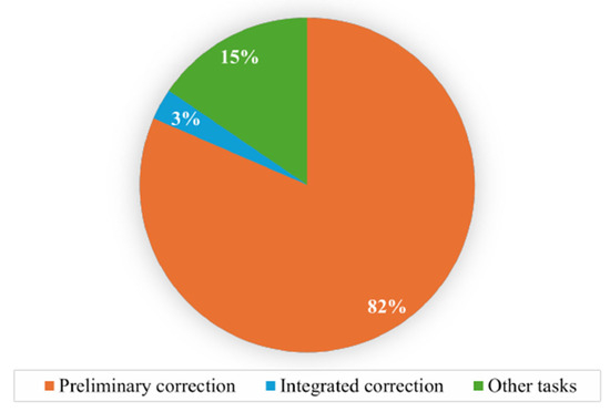
Figure 15.
Computing time breakdown of MECA for serial lines with and .
6. Conclusions and Future Work
In this paper, we present a novel approach to detect and correct errors in the parts flow data of serial production lines that are subject to measurement noise. To address this problem in the two-workstation case, we propose and develop an effective data-block-based algorithm to detect and then correct such data errors. As shown by numerical experiments, this algorithm can successfully correct most errors and restore data quality upon completion, leading to improved accuracy in performance metrics estimation.
To extend the data correction approach to multi-workstation cases, a two-stage decomposition/aggregation-based approach is proposed. Specifically, we first decompose an M-workstation line into two-workstation-line subsystems and apply the developed two-workstation case algorithm to each subsystem. Then, we aggregate the two-workstation-line subsystems, after preliminary correction, back to the original M-workstation serial line. Finally, the merged dataset is corrected using a newly developed algorithm, referred to as MECA during the integrated correction stage. Numerical experiments show that this approach can effectively detect and correct data errors in multi-workstation production lines.
The results of this work provide a theoretical foundation for reconstructing time series data with errors in manufacturing applications and contribute to improving data quality in manufacturing systems. These improvements can support more effective and accurate production planning, bottleneck identification, and maintenance scheduling in manufacturing environments. By reducing data-driven uncertainty, the method contributes to higher operational reliability and lower production costs, providing large benefits for smart manufacturing systems that rely on accurate data analytics. Future work includes extending the data detection criteria and data correction algorithms to other production lines and workstation reliability models such as exponential models. Additionally, we plan to extend our approach to other noise models and system structures to make it applicable in a wider range of settings. Moreover, improvement and optimization of the data correction algorithms will be explored to further improve its accuracy and computational efficiency. Finally, it should be noted that the results presented in this paper have the potential to be extended to other engineering applications that have noise-affected, discrete time series data measurements.
Author Contributions
Conceptualization, T.Z. and L.Z.; methodology, T.Z.; software, T.Z. and Y.B.; validation, T.Z., Y.B. and L.Z.; formal analysis, T.Z., Y.B. and L.Z.; investigation, T.Z. and L.Z.; resources, T.Z. and Y.B.; data curation, T.Z. and Y.B.; writing—original draft preparation, T.Z., Y.B. and L.Z.; writing—review and editing, T.Z. and L.Z.; visualization, T.Z.; supervision, L.Z.; project administration, L.Z.; funding acquisition, L.Z. All authors have read and agreed to the published version of the manuscript.
Funding
This research was funded by the U.S. National Science Foundation under Grant Number FM-2134367.
Data Availability Statement
No new data were generated in this research. All results are based on simulation outputs described in the manuscript.
Conflicts of Interest
The authors declare no conflicts of interest, except that Liang Zhang have financial interests and/or other relationships with Smart Production Systems LLC, Ann Arbor, MI, USA.
Appendix A. Other Noise Model Results
To validate the effectiveness and robustness of our method, we have also tested it under other noise models. The results of a few represented ones are given below:
- Noise Model 3
- Noise Model 4
Noise Models 3 and 4 extend Models 1 and 2 by allowing the error probability q to vary as a function of the true parts flow data, as illustrated in Figure A1. Specifically, these models capture scenarios where errors are less likely to occur when buffer occupancy is low, with the error probability decreasing linearly as occupancy decreases. The coefficient C controls how rapidly the error probability decreases with lower buffer occupancy. A moderate value ensures that the model reflects realistic sensitivity of sensor errors to operating conditions, too small a value would make the error probability nearly uniform, while too large a value would cause unrealistically steep decay. The selected value 0.03 represents a balanced setting. Figure A1. Example of probability of measured parts flow deviating from true values under Noise Model 3 and 4 ().Figure A1. Example of probability of measured parts flow deviating from true values under Noise Model 3 and 4 ().
- Noise Model 5
In Noise Model 5, when an error occurs, the measured value is drawn from a discrete Laplace distribution centered around the true value. The distribution is scaled by a normalization constant to ensure the total probability sums to 1, as shown in Figure A2. The coefficient determines how rapidly the probability decreases with increasing deviation. A larger causes the exponential term to decay faster, implying that large deviations are less likely, whereas a smaller results in a heavier-tailed distribution and greater noise intensity. Here was chosen to provide a balanced trade-off between concentration and variability, ensuring that the simulated measurement noise reflects realistic uncertainty levels observed in discrete manufacturing data.

Figure A2.
Example of probability distribution of under Noise Model 5 .
Figure A2.
Example of probability distribution of under Noise Model 5 .

The results for these models are summarized in Table A1. Compared with the results for Noise Models 1 and 2 presented in the main text, Table A1 shows similar trends under more complex noise models. The large estimation errors of and computed from raw data are reduced after applying the proposed correction method, and the discrepancy between the corrected and true data entries is also greatly diminished. However, although Noise Models 3 and 4 are extensions of Models 1 and 2, their error reduction is less pronounced. This is because the likelihood of errors is lower when buffer occupancy is small, limiting the number of correctable errors in these settings.
Table A1.
Average estimation error of performance metrics for ten-workstation lines under other noise models.
Table A1.
Average estimation error of performance metrics for ten-workstation lines under other noise models.
| q | 0.05 | 0.1 | 0.15 | 0.2 | 0.05 | 0.1 | 0.15 | 0.2 |
|---|---|---|---|---|---|---|---|---|
| Bernoulli line (Noise Model 3) | Geometric line (Noise Model 3) | |||||||
| 4.75% | 10.14% | 16.05% | 22.26% | 7.24% | 14.60% | 19.33% | 27.02% | |
| 0.33% | 1.64% | 2.59% | 4.06% | 0.25% | 1.12% | 2.54% | 5.26% | |
| 1.56% | 2.91% | 4.21% | 5.77% | 2.08% | 3.80% | 5.37% | 7.11% | |
| 1.12% | 2.48% | 3.90% | 5.26% | 0.92% | 2.07% | 3.27% | 4.36% | |
| 0.14% | 0.87% | 1.32% | 1.67% | 0.05% | 0.31% | 0.79% | 1.13% | |
| 0.82% | 1.06% | 1.33% | 1.66% | 1.42% | 1.67% | 1.96% | 2.37% | |
| 3.21% | 8.06% | 12.93% | 17.74% | 3.16% | 8.02% | 12.96% | 17.58% | |
| 0.70% | 4.30% | 8.24% | 11.07% | 0.39% | 2.80% | 6.32% | 10.04% | |
| 2.65 | 2.68 | 2.70 | 2.71 | 4.73 | 4.78 | 4.79 | 4.81 | |
| 1.27 | 1.29 | 1.31 | 1.32 | 1.47 | 1.51 | 1.56 | 1.61 | |
| Bernoulli line (Noise Model 4) | Geometric line (Noise Model 4) | |||||||
| 3.21% | 6.60% | 9.08% | 14.06% | 5.06% | 9.41% | 13.52% | 16.88% | |
| 0.43% | 1.80% | 2.71% | 4.03% | 0.22% | 1.40% | 3.28% | 5.63% | |
| 1.58% | 2.93% | 4.36% | 5.70% | 2.13% | 3.82% | 5.42% | 7.24% | |
| 0.93% | 1.88% | 2.98% | 4.10% | 0.65% | 1.43% | 2.18% | 3.25% | |
| 0.23% | 0.95% | 1.50% | 1.83% | 0.07% | 0.43% | 0.92% | 1.50% | |
| 0.88% | 1.15% | 1.44% | 1.80% | 1.54% | 1.83% | 2.18% | 2.65% | |
| 3.27% | 8.20% | 13.07% | 17.58% | 3.24% | 8.19% | 13.08% | 18.05% | |
| 1.18% | 2.80% | 6.32% | 10.04% | 0.58% | 3.88% | 7.29% | 11.58% | |
| 1.85 | 1.86 | 1.86 | 1.87 | 3.22 | 3.24 | 3.24 | 3.27 | |
| 1.17 | 1.21 | 1.27 | 1.31 | 1.39 | 1.46 | 1.51 | 1.60 | |
| Bernoulli line (Noise Model 5) | Geometric line (Noise Model 5) | |||||||
| 5.75% | 10.40% | 15.61% | 21.44% | 6.19% | 10.52% | 15.91% | 21.63% | |
| 1.90% | 2.89% | 3.61% | 4.72% | 2.02% | 3.92% | 5.30% | 7.11% | |
| 2.13% | 3.44% | 4.82% | 6.60% | 2.86% | 4.39% | 6.16% | 7.92% | |
| 0.95% | 1.83% | 2.78% | 3.80% | 0.55% | 1.09% | 1.54% | 2.13% | |
| 0.59% | 1.22% | 1.78% | 2.32% | 0.36% | 0.87% | 1.16% | 1.61% | |
| 0.59% | 0.92% | 1.24% | 1.59% | 0.78% | 1.21% | 1.63% | 2.09% | |
| 4.97% | 9.88% | 14.83% | 19.82% | 4.98% | 9.88% | 14.84% | 19.89% | |
| 3.58% | 6.82% | 9.87% | 13.02% | 3.33% | 6.53% | 10.09% | 13.88% | |
| 1.83 | 1.83 | 1.84 | 1.86 | 2.19 | 2.20 | 2.20 | 2.22 | |
| 1.27 | 1.29 | 1.29 | 1.31 | 1.48 | 1.50 | 1.53 | 1.55 | |
For Noise Model 5, the correction method also achieves notable reductions in the estimation errors of and and in the overall data discrepancy. Nonetheless, since the sensor is more likely to return values distributed around the true data, it becomes more difficult to distinguish erroneous entries. As a result, the average fraction of inconsistent entries after correction () is higher, because many errors are subtle and closely resemble the true values.
To verify the robustness, a sensitivity analysis was conducted. As defined in Equations (A9) and (A10), the relative improvement metrics were used for evaluation. The corresponding results are presented in Figure A3, Figure A4 and Figure A5. For Noise Models 3 and 4, varying the coefficient C results in only minor changes in the relative improvement for both Bernoulli and Geometric models, indicating that the method is robust to different decay rates of the error probability. In Noise Model 5, increasing leads to a gradual decrease in the improvement indices, corresponding to reduced noise intensity.

Figure A3.
Sensitivity of improvement with respect to C (Noise Model 3, ).
Figure A3.
Sensitivity of improvement with respect to C (Noise Model 3, ).


Figure A4.
Sensitivity of improvement with respect to C (Noise Model 4, ).
Figure A4.
Sensitivity of improvement with respect to C (Noise Model 4, ).


Figure A5.
Sensitivity of improvement with respect to (Noise Model 5, ).
Figure A5.
Sensitivity of improvement with respect to (Noise Model 5, ).

These results confirm that the improvements demonstrated in the main text are not limited to specific scenarios. We further evaluated the metrics under various parameter settings and additional noise models, and consistently observed similar improvements in estimation accuracy and robustness. These extended experiments reinforce the conclusion that the proposed correction method generalizes well and is suitable for deployment in real-world production lines with diverse noise characteristics and system configurations.
References
- Rojko, A. Industry 4.0 concept: Background and overview. Int. J. Interact. Mob. Technol. 2017, 11, 5. [Google Scholar] [CrossRef]
- Javaid, M.; Haleem, A.; Singh, R.P.; Suman, R. An integrated outlook of cyber–physical systems for Industry 4.0: Topical practices, architecture, and applications. Green Technol. Sustain. 2023, 1, 100001. [Google Scholar] [CrossRef]
- Wang, S.; Wan, J.; Zhang, D.; Li, D.; Zhang, C. Towards Smart Factory for Industry 4.0: A self-organized multi-agent system with big data based feedback and coordination. Comput. Netw. 2016, 101, 158–168. [Google Scholar] [CrossRef]
- Kusiak, A. Smart manufacturing. Int. J. Prod. Res. 2018, 56, 508–517. [Google Scholar] [CrossRef]
- Sun, Y.; Zhu, T.; Zhang, L.; Denno, P. Parameter identification for Bernoulli serial production line model. IEEE Trans. Autom. Sci. Eng. 2020, 18, 2115–2127. [Google Scholar] [CrossRef]
- Tu, J.; Zhu, T.; Bai, Y.; Zhang, L. Estimation of machine parameters in exponential serial lines using feedforward neural networks. In Proceedings of the 2020 IEEE 16th International Conference on Automation Science and Engineering (CASE), Virtual, 20–21 August 2020; pp. 816–821. [Google Scholar]
- Sun, Y.; Zhang, L. Application of a novel approach of production system modelling, analysis and improvement for small and medium-sized manufacturers: A case study. Int. J. Prod. Res. 2023, 61, 3279–3299. [Google Scholar] [CrossRef]
- Qin, S.J.; Dong, Y.; Zhu, Q.; Wang, J.; Liu, Q. Bridging systems theory and data science: A unifying review of dynamic latent variable analytics and process monitoring. Annu. Rev. Control 2020, 50, 29–48. [Google Scholar] [CrossRef]
- Ait-El-Cadi, A.; Gharbi, A.; Dhouib, K.; Artiba, A. Integrated production, maintenance and quality control policy for unreliable manufacturing systems under dynamic inspection. Int. J. Prod. Econ. 2021, 236, 108140. [Google Scholar] [CrossRef]
- Maleki, M.R.; Amiri, A.; Castagliola, P. Measurement errors in statistical process monitoring: A literature review. Comput. Ind. Eng. 2017, 103, 316–329. [Google Scholar] [CrossRef]
- Chen, L.P.; Yang, S.F. A new p-control chart with measurement error correction. Qual. Reliab. Eng. Int. 2023, 39, 81–98. [Google Scholar] [CrossRef]
- Oleghe, O. A predictive noise correction methodology for manufacturing process datasets. J. Big Data 2020, 7, 89. [Google Scholar] [CrossRef]
- Teh, H.Y.; Kempa-Liehr, A.W.; Wang, K.I.K. Sensor data quality: A systematic review. J. Big Data 2020, 7, 11. [Google Scholar] [CrossRef]
- Ju, F.; Li, J.; Horst, J.A. Transient analysis of serial production lines with perishable products: Bernoulli reliability model. IEEE Trans. Autom. Control 2016, 62, 694–707. [Google Scholar] [CrossRef] [PubMed]
- Yan, F.; Wang, J.; Li, Y.; Cui, P. An improved aggregation method for performance analysis of Bernoulli serial production lines. IEEE Trans. Autom. Sci. Eng. 2020, 18, 114–121. [Google Scholar] [CrossRef]
- Dong, H.; Li, J. Modeling and analysis of productivity and energy in serial production lines with setups. IEEE Trans. Autom. Sci. Eng. 2023, 22, 18102–18117. [Google Scholar] [CrossRef]
- Wang, X.; Dai, Y.; Jia, Z. Energy-efficient on/off control in serial production lines with Bernoulli machines. Flex. Serv. Manuf. J. 2024, 36, 103–128. [Google Scholar] [CrossRef]
- Lee, J.H.; Li, J.; Horst, J.A. Serial production lines with waiting time limits: Bernoulli reliability model. IEEE Trans. Eng. Manag. 2017, 65, 316–329. [Google Scholar] [CrossRef]
- Kang, N.; Ju, F.; Zheng, L. Transient analysis of geometric serial lines with perishable intermediate products. IEEE Robot. Autom. Lett. 2016, 2, 149–156. [Google Scholar] [CrossRef]
- Zhu, T.; Zhang, L. Detection and correction of buffer occupancy data error in two-machine Bernoulli serial lines. In Proceedings of the 2022 IEEE 18th International Conference on Automation Science and Engineering (CASE), Mexico City, Mexico, 20–24 August 2022; pp. 1854–1859. [Google Scholar]


Disclaimer/Publisher’s Note: The statements, opinions and data contained in all publications are solely those of the individual author(s) and contributor(s) and not of MDPI and/or the editor(s). MDPI and/or the editor(s) disclaim responsibility for any injury to people or property resulting from any ideas, methods, instructions or products referred to in the content. |
© 2025 by the authors. Licensee MDPI, Basel, Switzerland. This article is an open access article distributed under the terms and conditions of the Creative Commons Attribution (CC BY) license (https://creativecommons.org/licenses/by/4.0/).