Addressing Real-World Localization Challenges in Wireless Sensor Networks: A Study of Swarm-Based Optimization Techniques

Abstract

Wireless sensor networks (WSNs) have gained significant attention across various industries and scientific fields. Localization, a crucial aspect of WSNs, involves accurately determining node positions to track events and execute actions. Despite the development of numerous localization algorithms, real-world environments pose challenges such as anisotropy, noise, and faults. To improve accuracy amidst these complexities, researchers are increasingly adopting advanced methodologies, including soft computing, software-defined networking, maximum likelihood estimation, and optimization techniques. Our comprehensive review from 2020 to 2024 reveals that approximately 29% of localization solutions employ optimization techniques, 48% of which utilize nature-inspired swarm-based algorithms. These algorithms have proven effective for node localization in a variety of applications, including smart cities, seismic exploration, oil and gas reservoir monitoring, assisted living environments, forest monitoring, and battlefield surveillance. This underscores the importance of swarm intelligence algorithms in sensor node localization, prompting a detailed investigation in our study. Additionally, we provide a comparative analysis to elucidate the applicability of these algorithms to various localization challenges. This examination not only helps researchers understand current localization issues within WSNs but also paves the way for enhanced localization precision in the future.

1. Introduction

In recent years, nature-inspired optimization algorithms have gained traction for addressing real-world challenges across diverse domains, such as aeronautics, robotics, power systems, medical imaging, localization, and various engineering optimization problems [1,2,3]. These algorithms are inspired by the efficient methods that nature uses to solve complex tasks. They are problem-independent methods that can be used as black boxes. Given the objective function and the constraints, they attempt to provide the best possible solution within the given search area.

Wireless sensor networks (WSNs) extensively employ optimization algorithms to increase network performance. A WSN is a network of sensor nodes that are used for data collection from remote locations. A typical sensor node consists of sensors for sensing the environment, a power source, a memory unit for storing data, an embedded processor for data processing, and a transceiver unit for exchanging data with other nodes. The critical technologies of WSNs include network topology control, routing, QoS assurance, location awareness, data fusion, and data management.

These networks face several challenges in the various phases of their operations. Localization is one of the crucial challenges faced by WSNs. This is the task of identifying the locations of nodes. Typically, the sensing region is remote, large, and unreachable, and nodes are deployed randomly. Hence, their locations are unknown to the network administrator. However, to analyze and act on the received events, the location information of nodes is critical. In real-world scenarios, the presence of obstacles, varying environmental conditions, and noise add to the complexity of these algorithms.

Researchers have developed numerous techniques to achieve accurate node localization under various conditions, which are broadly categorized into anchor-free and anchor-based localization. In anchor-free localization, only the estimated distances between nodes are known, and a relative map of the nodes is generated based on this information. The second type, anchor-based localization, involves estimating the distances between unknown nodes and anchor nodes using measurements such as received signal strength (RSS), time of arrival (TOA), time difference in arrival (TDOA), and hop distance—i.e., the number of hops required for a signal to travel from an anchor node to an unknown node. Localization is then performed using methods such as centroid, triangulation, trilateration, and approximate point-in-triangle techniques.

These are simple methods and are more suitable for ideal scenarios. The accuracy of these methods deteriorates in real field environments with obstacles and noise interference. To improve accuracy in such scenarios, researchers are using more advanced techniques, such as soft computing techniques, the Fermat point model, software-defined network techniques, the maximum likelihood estimation method, and optimization techniques.

We have conducted a detailed analysis of the various types of localization techniques using dimension databases from 2020 to 2024 [4]. Around 2100 papers were selected using the keywords “wireless sensor network” and “localization”. From these, approximately 600 papers were further identified using the additional keyword “optimization”. These papers were then manually reviewed to identify publications that employed swarm-based optimization techniques. It was observed that approximately 29% of the solutions are provided via optimization techniques, and 48% of these solutions use swarm-based optimization techniques, as shown in Figure 1. This trend underscores the rising prominence of swarm-based algorithms for localization challenges. These algorithms iteratively generate and refine the sets of possible solutions to converge toward optimal outcomes.

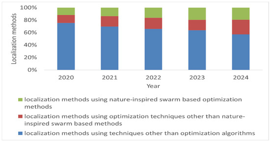
Figure 1. An analysis of localization methods.

This paper aims to present a comparative study elucidating how optimization algorithms can be applied to diverse localization challenges. This examination not only helps researchers grasp current localization issues within WSNs but also charts pathways for achieving heightened localization precision in the future. In addition to comparing the performance and effectiveness of optimization algorithms, this paper also investigates their adaptability to different environmental conditions and network topologies. Understanding how these algorithms behave in various scenarios is crucial for their practical implementation in real-world wireless sensor networks. Moreover, this paper delves into the challenges and limitations encountered when applying nature-inspired optimization algorithms for sensor node localization. By identifying and addressing these issues, researchers can develop more robust and reliable localization techniques that can withstand diverse network conditions and deployment scenarios. Overall, this comprehensive analysis serves as a valuable resource for researchers and practitioners in the field of wireless sensor network localization, offering insights into the current state of the art and highlighting potential avenues for future advancements.

This paper is organized as follows. Section 2 provides an analysis of the commonly faced problems in localization. A comparison of the various inspirations for swarm-based algorithms is described in Section 3. The application of these algorithms for different localization problem domains is presented in Section 4. Section 5 provides the conclusion and future directions.

2. Problem Domains in Localization of WSNs

WSNs have a wide range of applications, from oil, gas, and military to healthcare and precision agriculture. The accurate identification of the locations of nodes in these real-world applications has many challenges. Based on a thorough review of the literature, we identified a list of commonly faced problems in localization.

• Deployment terrain:

Node localization in a WSN deployed on a 2D plain ground is a straightforward task. One example is a location-unknown node that can estimate its distance to three nonlinear anchor nodes by measuring the RSS or time or angle of arrival of signals from these anchor nodes. Then, the location of the node can be estimated as the centroid of the intersection area of three circles drawn by keeping the anchor node as the center and the distance as the radius. This is illustrated in Figure 2.

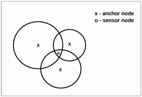
Figure 2. Node localization via the centroid method.

However, in actual applications, nodes are rarely deployed in 2D plain fields. In the case of oil and gas applications, the deployment field may consist of mountain terrains, and in the case of healthcare applications, sensor nodes may have to be deployed in multifloored buildings. The localization of nodes in such 3D terrains is more complex. For localization in 3D fields, sensor nodes need to know the distance from at least four anchor nodes. The node can identify its location as the centroid of the intersection of four spheres drawn by keeping these anchor nodes as centers. Three-dimensional operations increase the computational cost of the localization algorithms.

• Obstructions:

The initial step of any existing localization technique is to estimate the distance of the unknown sensor nodes from the anchor nodes. This is achieved by nodes exchanging signals with each other and measuring the characteristics of the received signal. The characteristics can be the RSS, or the time it takes for a signal to travel from the sending node to the receiving node, or it can be just because the unknown node is within the communication range of the reference node. As shown in Figure 3, the presence of obstructions in the field affects these signal characteristics and hence deteriorates the distance estimation between nodes, which in turn reduces the accuracy of the localization algorithms.

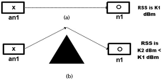
Figure 3. Effect of obstacles on RSS measurements (a) without obstacles (b) with obstacles.

• Noise:

In addition to obstructions, signal transmission between nodes is also affected by environmental conditions such as rain, vegetation, and sandstorms. This noise contribution needs to be considered using appropriate channel models, such as path loss log-normal models, while developing localization algorithms.

• Energy consumption:

Sensor nodes normally operate on batteries with limited energy. As the nodes are deployed in remote locations, there is no possibility of recharging or replacing the batteries. Hence, power consumption is a major concern for WSNs operating in remote locations. Algorithms with higher computational complexity and communication overheads may drain the battery, reducing the lifetime of the network.

• Hardware requirements:

Few localization algorithms require additional information, such as the TOA, TDOA, and angle of arrival (AOA), for the accurate localization of nodes. However, this information is not readily available with nodes. In such cases, nodes need to be attached to additional hardware equipment, which increases the size and energy consumption of nodes.

These problem domains must be addressed while developing localization algorithms. Optimization techniques provide promising results in addressing these problem areas.

3. Optimization Algorithms

Optimization algorithms are used to find optimal solutions from a set of possible solutions via objective functions [5]. Optimization algorithms can generally be classified as deterministic or heuristic algorithms. Deterministic techniques exploit analytical capabilities, whereas heuristic techniques are probabilistic methods. The swarm-based optimization algorithms are heuristic algorithms. These are inspired by the collective intelligence of various biological systems.

3.1. General Workflow

Swarm-based algorithms follow a set of common steps. In the initial step, they generate a set of random candidate solutions, which are referred to as the population. The quality of the generated solutions is evaluated via a cost function. The cost function depends on the requirements of the user. The user of the optimization algorithm must define the cost function such that when the algorithm obtains a solution with minimal cost, it becomes the optimal solution. These solutions are then iteratively updated in various phases, such as exploration and exploitation, to converge at a global optimum solution. The solution with the least cost is identified as the best solution. The steps are illustrated in Figure 4.

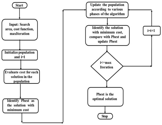
Figure 4. General flow chart of swarm-based optimization algorithms.

3.2. A Comparison of the Various Inspirations for Optimization Algorithms

In recent years, researchers have developed optimization algorithms by mathematically modeling various natural behaviors [6,7,8,9]. However, theoretically, it is not possible to consider any optimization algorithm as the best general-purpose algorithm. Hence, new optimizers with specific global and local search strategies continue to emerge to provide a greater variety of choices for researchers and experts in different fields.

These algorithms initially identify random candidate solutions within the acceptable range. These candidate solutions are then iteratively updated in the exploration and exploitation phases, which are represented by mathematically modeling various natural behaviors. The exploration phase searches for better solutions in the entire region, whereas exploitation search is a more focused search in a small region [10]. These optimization algorithms can be used in a variety of applications. According to the needs of each application, a cost function must be defined for evaluating the fitness of the candidate solutions. The solution producing the lowest cost value is identified as the optimal solution.

In this section, we compare and discuss various inspirations for optimization algorithms that are popularly used to solve localization problems. Particle swarm optimization (PSO) is a popular search algorithm designed by mathematically modeling birds seeking food [11]. Here, each bird is referred to as a particle. Initially, several particles are randomly placed within the search space of the given problem. Each particle then evaluates the cost value at its current location. The particle producing the minimum cost value is identified as the best solution. Each particle then updates its velocity and position as a function of its own current location, its previous best position, and the identified best position among all the particles along with some random perturbations. These steps are repeated until the solutions converge to the best possible solution within the defined maximum number of iterations [12]. This powerful optimization algorithm is popularly used in a wide range of applications, such as image and video analysis, the design and restructuring of electricity networks and load dispatching, control applications, sensors and sensor networks, etc. [13].

The gray wolf optimizer (GWO) was derived by modeling the social hierarchy and hunting behavior of gray wolves [14]. Gray wolves, which are at the top of the food chain, follow a very interesting social hierarchy. The leaders of the pack are called alpha wolves, the subordinates to the alpha wolves are called beta wolves, the elders, hunters, and scout wolves are called deltas, and the omega wolves are in the lowest rank. This hierarchy is mathematically modeled in the GWO algorithm. The fittest solution among a set of candidate solutions is mapped as alpha, and the second- and third-best solutions are mapped as beta and delta, respectively. The remaining candidate solutions are mapped as omegas. The step toward obtaining the optimal solution is modeled via the search for prey and the hunting behavior of gray wolves. The search for prey is a global search through exploration that avoids stagnation at local solutions, whereas hunting prey is a more intense local search. These steps are repeated to converge toward an optimal solution.

Harris hawk optimization (HHO) has taken inspiration from the cooperative behavior and chasing style of Harris hawks [15]. Hawks are among the most intelligent birds in nature. For hunting, they perch randomly on some locations by considering the locations of other family members and waiting to detect prey. In this algorithm, this behavior is modeled as an exploration phase. The hawks are the candidate solutions, and the intended prey is the best candidate solution in each step. Once the intended prey is detected, hawks perform a surprise pounce, which is modeled as the exploitation phase. The transition from the exploration to exploitation phase occurs based on the energy of the prey. The energy of the prey is modeled as a function of time and is found to decrease with increasing time. After some time, prey will lose more energy, and hawks intensify the hunting process to effortlessly catch the prey. This leads us to the best optimal solution. This is a population-based algorithm that can be applied to any field by properly formulating the problem.

The artificial hummingbird algorithm (AHA) is another optimization algorithm that simulates special flight skills, superior memory, and intelligent foraging strategies of hummingbirds in nature [16]. This algorithm uses a distinct memory update mechanism with a visit table, which makes it quite different from the other algorithms. Here, each hummingbird is assigned to a specific food source. Food sources are candidate solutions, and the nectar refilling rate of a food source determines the fitness value of the solution.

The bat optimization algorithm (BOA) is an algorithm that functions based on the echo-locating behavior of bats [17]. The artificial gorilla trout optimizer (AGTO), which is inspired by the social intelligence of gorilla troops, has also shown improved localization performance. Another metaheuristic algorithm based on the collaborative hunting strategy of penguins, the penguin search optimization (PenSO) algorithm, is also useful for solving localization problems.

Many more optimization algorithms have been developed by taking inspiration from natural behaviors. These algorithms are developed from the concept of the no free lunch (NFL) theorem proposed by Wolpert and Macready [18]. Accordingly, different algorithms are suitable for solving different problems. There is no single optimization algorithm that can solve all varieties of problems.

A comparison of various optimization algorithms is provided in Table 1.

Table 1. Comparison of nature-inspired optimization algorithms.

Algorithm	Inspiration	Experiments	Evaluation Criteria	Remarks	Applications
PSO [11]	The cooperative behavior of a swarm of bees searching for food	A benchmark for genetic algorithms: the extremely nonlinear Schaffer f6 function.	Global optimum	Simple, easy to implement, computationally efficient.	To solve wireless communications optimization problems, image processing, and electrical power systems [13]
GWO [14]	Leadership hierarchy and hunting mechanism of gray wolves	In total, 23 classical benchmark functions, 6 composite benchmark functions from CEC2005, and engineering problems: tension/compression spring, welded beam, and pressure vessel designs.	Exploration and exploitation ability, local optima avoidance, and convergence using average and standard deviation statistical results	Superior exploitation and high local optima avoidance.	Searching for the best set of features in data mining applications, in design and tuning controllers, for optimizing robot path planning [19]
HHO [15]	Exploring prey, surprise pounce, and different attacking strategies of Harris’ hawks	Three main groups of benchmark landscapes: unimodal, multimodal, composition, and engineering problems: three-bar truss, tension spring, pressure vessel, welded beam, multi-plate disk clutch brake, and rolling element bearing.	Wilcoxon statistical test with 5% degree of significance with swarm size and maximum iterations of all optimizers set to 30 and 500	Accelerated convergence trend and scalable.	Detection of COVID-19 severity, diabetic retinopathy, and parameter identification of photo voltaic systems, predicting the compressive strength of green concretes [20,21,22,23]
AHA [16]	The special flight skills and intelligent foraging strategies of hummingbirds	In total, 50 benchmark functions with unimodal, multimodal, non-separable and separable characteristics, and 10 engineering cases.	Wilcoxon signed-rank test with mean and standard deviation analysis	Scalable to high-dimensional functions, superior exploration ability, and better performance in multimodal and separable functions.	To solve engineering design problems and to predict the wear rates of various nanocomposites [24,25]
BOA [17]	Based on the echolocation behavior of bats	Eight design problems: mathematical problem, Himmelblau’s problem, three-bar truss design, speed reducer design, parameter identification of structures, cantilever stepped beam, heater exchanger design, and car side problem.	Statistical analysis of best, mean, worst, and standard deviation	Efficient, superior performance and more powerful.	For solving economic dispatch problems in power systems and MRI image segmentation [26,27]
AGTO [28]	Gorilla troops’ social intelligence in nature	Benchmark functions, including three different unimodal, multimodal, and composite groups.	The best solution, the worst solution, standard deviation, and average mean with 30 populations in a maximum of 500 iterations	Provides better solutions with better convergence than its competitors and can be applied to real-world case studies with unknown search spaces.	To optimize the parameters of the PID controller, parameter extraction of the PV model, and parameter extraction of the proton exchange membrane fuel cells [29,30,31]
PenSO [32]	Collaborative hunting strategy of penguins	De Jong function, Rosenberg function, Schwefel Function, and Michalewicz function.	Convergence of the algorithm	Robust and efficient, it can detect all local minima and the global minimum in the search space.	To solve the quadratic assignment problem, for biomedical data classification, and community detection in complex networks [33,34,35]
Improved Fish Migration Optimization (FMO) [36]	Simulates the predation and growth process of fish	Four benchmark unimodal and multimodal functions.	Convergence, accuracy and speed with 2000 iterations and a population size of 20	Fast convergence rate and has good global search capabilities.	To solve unit commitment problem of power system and PID parameter tuning [37,38]
Bald Eagle Search Optimization (BESO) Algorithm [39]	Mimics the hunting strategy of bald eagles as they search for fish	Thirty benchmark functions of the CEC2014 on Single Objective Real-Parameter Numerical Optimization, and twenty-five benchmark functions of the CEC 2005.	Mean, standard deviation, best point, and Wilcoxon signed-rank test statistic of the function values	Has shown better performance in unimodal, multimodal, hybrid, and expanded functions. However, performance was not very satisfactory in scenarios with multiple local optima.	For parameter estimation of different photovoltaic models, optimal parameter identification of super capacitor model [40,41]
Sparrow Search Algorithm (SSO) [42]	Inspired by the group wisdom, foraging, and anti-predation behaviors of sparrows	Nineteen standard test functions and two practical engineering problems: Himmelblau’s nonlinear optimization problem and Speed reducer design.	Convergence speed, stability, and accuracy by setting the maximum number of iterations to 1000 and the population size to 100	High performance in diverse search spaces and local optimum issues is avoided effectively.	3D route planning for UAV; path planning for mobile robots [43,44]
Bird Swarm Optimization (BSO) Algorithm [45]	Based on the behavior of bird swarms and respective hierarchical order	Eighteen benchmark problems containing unimodal, multimodal, high-dimensional, and low-dimensional cases.	Optimization accuracy, best fitness, and convergence time with 100 independent trials with 1000 iterations	Reduced the local optimal solutions and improved global solution.	Load balancing for cloud computing environment [46]
Cat Swarm Optimization (CSO) [47]	Inspired by the behavior of cats by mimicking the tracing mode and seeking mode	Six test functions namely Rastrigrin, Griewank, Ackley, Axis parallel, Trid10, and Zakharov.	Fitness value and process time	Can produce better solutions a reduced time.	Alcohol use disorder identification in adaptive identification of infinite impulse response systems [48,49]
Whale Optimization Algorithm (WOA) [50]	Inspired by the hunting behavior of hump-back whales	Twenty-nine mathematical optimization problems and six constrained engineering design problems; namely, a compression spring, a welded beam, a pressure vessel, a 15-bar, a 25-bar, and a 52-bar truss.	Average cost function and corresponding standard deviation were tested with a population size of 30 and a maximum iteration of 500	Better exploration, exploitation, local optima avoidance, and convergence behavior.	Resource allocation in wireless networks for medical feature selection [51,52]

4. Optimization Algorithms for Solving the Localization Problem

Optimization algorithms have been found to be very effective in solving the various problem domains of WSN localization. Any localization problem can be represented mathematically, and suitable optimization algorithms can be applied to solve this efficiently. A few popular optimization algorithms used to solve the localization problem are shown in Figure 5.

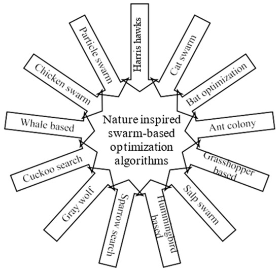
Figure 5. Nature-inspired swarm-based optimization algorithm.

The general workflow of the existing optimization-based localization algorithms is discussed here.

Steps:

1.

Initially, the locations of unknown nodes are deployed randomly in the required field along with a few locations known as anchor nodes. These anchor nodes are placed in predefined locations or are attached to GPS receivers.

2.

The distances of unknown nodes to anchor nodes are estimated via range-based techniques such as RSSI, time of arrival, time difference in arrival, etc., or range-free techniques such as hop count-based distance estimation. In range-based techniques, unknown nodes estimate their distance to anchor nodes via signal characteristics such as received signal strength or the time a signal takes to travel from the anchor to unknown nodes. In range-free techniques, parameters such as the minimum number of intermediate nodes required for the anchor node to communicate with an unknown node are used to estimate the distance from unknown nodes to anchor nodes. However, these distance estimates can be erroneous because of obstructions, environmental noise, and irregular field dimensions.

3.

Next, these distance estimates are used to define the objective function.

The advantage of using optimization techniques over other methods for solving the problem of localization is that the effect of erroneous distance estimations due to anisotropic fields and noisy conditions on the localization accuracy can be drastically reduced. This is because optimization algorithms try to provide the best optimal result from the available multiple erroneous results. For example, consider a scenario with three anchor nodes located at (x_j, y_j), where j = 1 to 3, and one unknown node with an unknown location ($\overline{x_1}$, $\overline{y_1}$) in a network. Let d_1j represent the estimated erroneous distance between the unknown node 1 and anchor node j. The Distance Vector Hop (DVHop) algorithm tries to find the value of ($\overline{x_1}$, $\overline{y_1}$) by solving the following equation.

$$\begin{gathered} {\left(\overline{x_1}-x_1\right)}^2+{\left(\overline{y_1}-y_1\right)}^2=d_{11}^2 \\ {\left(\overline{x_1}-x_2\right)}^2+{\left(\overline{y_1}-y_2\right)}^2=d_{12}^2 \\ {\left(\overline{x_1}-x_3\right)}^2+{\left(\overline{y_1}-y_3\right)}^2=d_{13}^2 \end{gathered}$$

(1)

Since d₁j is erroneous, the estimated location ($\overline{x_1}$, $\overline{y_1}$) will also be inaccurate. However, by properly formulating the objective function, optimization algorithms can be used to find the best possible estimate of ($\overline{x_1}$, $\overline{y_1}$), such that the errors in Equation (1) are minimized.

Optimization algorithms require objective functions to produce optimal solutions. The objective function is a representation of the overall goal of the problem. The representation of the localization problem as an objective function can be performed in different ways.

The most common method is shown in Equation (2). Here, N is the number of unknown nodes, M is the anchor node count, ($\overline{x_i}$, $\overline{y_i}$) is the estimated location of node i, (x_j, y_j) is the location of anchor node j, and d_ij is the estimated distance between node i and anchor node j.

$$F=Min {\sum }_{i=1, j=1}^{N, M}\left|\left(\sqrt{{\left(\overline{x_i}-x_j\right)}^2+{\left(\overline{y_i}-y_j\right)}^2}-d_{ij}\right)\right|$$

(2)

After the objective function is defined, the problem of estimating the coordinates ($\overline{x_i}$, $\overline{y_i}$) such that they result in the minimum value of F can be solved via various optimization algorithms. While Equation (2) is one way of representing the localization problem mathematically as an objective function, there are many other ways in which the localization problem can be represented, depending on the problem domain.

A novel mobile anchor node-based localization algorithm is defined in [53]. Here, using a mobile anchor node, a location-unknown node estimates its distance to a mobile anchor node at three noncollinear positions via RSSI measurements. Then, the initial location estimation for the unknown node is obtained via trilateration. These distance estimations are prone to corruption by noise. To overcome this problem, the search space is defined by considering the errors introduced by this noise. It is defined as the overlapping region of three circles drawn with the anchor node as the center and the obtained distance estimation as the radius.

The objective function is defined as

$$F={\displaystyle \frac{1}{M}} {\sum }_{j=1}^{ M}\left|\left(\sqrt{{\left(\overline{x_i}-x_j\right)}^2+{\left(\overline{y_i}-y_j\right)}^2}-d_{ij}\right)\right|$$

(3)

where M is the number of anchor signals received by location-unknown node i. This objective function is solved via an improved version of the PSO method called the FPSOTS method. The localization results revealed a performance improvement at varying anchor densities, noise effects, and anchor transmission ranges.

Noise, which is random in nature, normally affects distance estimation and, in turn, the localization accuracy of nodes. Ref. [54] reported a BOA-based localization algorithm for the localization of nodes by considering the effect of noise in the localization process. For this purpose, two variants of the bat optimization algorithm are developed by enhancing the exploration and exploitation characteristics. The initial location of an unknown node is defined as the average location of anchor nodes within the transmission region. Next, the objective function is defined as the mean square error:

$$F={\displaystyle \frac{1}{M}} {\left. {\sum }_{i=1}^{ M}\left(\sqrt{{\left(\overline{x_i}-x_j\right)}^2+{\left(\overline{y_i}-y_j\right)}^2}\right. -d_{ij}\right)}^2$$

(4)

This error is then reduced over multiple iterations by using the defined optimization algorithm.

To solve the problem of localization in the presence of obstacles [55], a gray wolf localization algorithm based on beetle antennae search (BASGWO) was reported. This algorithm estimates the distance from multiple anchor nodes to location-unknown nodes via the logarithmic-normal distribution model and signal strength measurements, as expressed in Equation (5).

$$P_t\left(d\right)=P_t\left(d_0\right)-10\eta .\mathit{log}\left({\displaystyle \frac{d}{d_0}}\right)+X_a$$

(5)

Here, P_t(d) is the received power at distance d, P_t(d₀) is the received power at distance d₀, η is the path loss factor, and $X_a$ is a random number with a mean of 0. Using these distance estimates, the objective function is defined as

$$F={\sum }_{i=1}^{ M}\left[\left|\sqrt{{\left(\overline{x_i}-x_j\right)}^2+{\left(\overline{y_i}-y_j\right)}^2}-d_{ij}\right|. {\displaystyle \frac{1}{d_{ij}}}\right]$$

(6)

A weight coefficient of ${\displaystyle \frac{1}{d_{ij}}}$ is considered here to compensate for the increase in distance estimation errors with increasing distance. This is then solved via an improved GWO algorithm called the BASGWO algorithm. The performance improvements were observed at varying node and anchor node ratios and at different communication radii.

To reduce the localization errors introduced due to the asynchronous nonuniform distribution of nodes, a novel parallel compact cat swarm optimization with DV-Hop (PCCSO-DV-Hop) is reported in [56]. Here, the distance estimation is initially performed using the average hop distance between nodes. The objective function is then formed as

$$F=Min \left({\sum }_{i=1}^M{{\left({\displaystyle \frac{1}{ho{p}_{ij}}}\right)}^2 \left(\sqrt{{\left(\overline{x_i}-x_j\right)}^2+{\left(\overline{y_i}-y_j\right)}^2}-d_{ij}\right)}^2\right)$$

(7)

Here, $ho{p}_{ij}$ is the number of hops between nodes i and j. This objective function uses the inverse of the number of hops to compensate for the errors introduced by distant nodes with larger hop values.

In [57], an AHA-based localization algorithm was defined to localize the nodes deployed in isotropic and anisotropic fields with obstacles. This algorithm aims to reduce the dependency on anchor nodes by using only two anchor nodes for the localization of the entire network. Then, a hop-based method is developed to identify a few more unknown nodes located as anchor nodes, and a hop-based distance estimation method is used for the initial distance estimation. The objective function is expressed as

$$F=Min {\sum }_{j=A, B, C, D}\left|\sqrt{{\left(\overline{x_i}-x_j\right)}^2+{\left(\overline{y_i}-y_j\right)}^2}-d_{ij}\right|$$

(8)

Here, $d_{ij}$ is the distance between sensor node i and four reference nodes A, B, C, and D. This problem is solved via the AHA. The results are then analyzed in various isotropic and anisotropic fields at various node densities. To reduce TDOA-based localization errors in 3D environments [18], an opposition-based learning and parallel strategy, AGTO, has been reported. Here, the objective function is calculated as

$$erro{r}_{1,i}=R_{i+1}-R_1+Nois{e}_1$$

(9)

$$erro{r}_{2,i}=D_{i+1}-D_1+Nois{e}_2$$

(10)

$$error={\sum }_{i=1}^{N-1}\sqrt{{\left(erro{r}_{1,i}-erro{r}_{2,i}\right)}^2}$$

(11)

R_i represents the distance from the unknown node to anchor node i, and D_i represents the distance from the algorithm-estimated node to anchor node i.

A comparison of optimization-based localization algorithms using range-free and range-based methods is provided in Table 2 and Table 3. These tables provide a summary of various swarm-based localization algorithms from the literature, highlighting the specific swarm optimization techniques used, the problem domains addressed by each algorithm, the variables considered for testing, and the corresponding analysis of results.

Table 2. Comparative analysis of range-free-based localization techniques for WSNs.

Algorithm	Optimization Algorithm	Problem Domain	Variables	Result Analysis
Harris Hawks optimization-based localization with area minimization (HHO-AM) [58]	HHO	2D and 3D regular and irregular fields with obstacles	Heterogeneity, irregularity, node density, and anchor node density	Showed improved accuracy when compared with DV-Hop, EWCL, and DV-maxHop
Artificial hummingbird algorithm-based localization method (AHAL) [57]	AHA	Isotropic and anisotropic fields with obstacles	Node density and type of field	Improved localization accuracy in comparison with DV-Hop, Weighted DV-Hop, HHO-AM, and PSO-based localization method
Improved FMO DV-Hop [59]	FMO	3D terrain with obstacles		Improved localization accuracy in comparison with DV Hop and PSO DV Hop
Crow search weighted centroid localization (CS- WCL) [60]	crows search algorithm	2D plain field	Communication radius, anchor nodes, and total nodes	Improved accuracy compared with DV-Hop and weighted centroid algorithm
Parallel compact CSO with DV-Hop [56]	CSO	2D plain field	Node density, anchor node density, and communication radius	Lowest localization error compared with PSO-DV-Hop, CSO-DV-Hop, CCSO-DV-Hop, and PCSO-DV-Hop
New DVHop cuckoo search (NDV-HopCS) [61]	cuckoo search algorithm	Square, H-shaped, and O-shaped random environments	Node density, anchor node percentage, and communication range	Improved localization accuracy when compared with DV-Hop, DV-HopPSO, and DV-HopCSO
Parallel and compact WOA [62]	WOA	2D plain field	Communication radius, anchor nodes, and total nodes	PCWOA showed improved performance compared with DV-Hop, PSO, WAO, and Parallel Whale Optimization Algorithm
Localization based on improved DVHop and improved GWO [63]	GWO	T-shaped, S-shaped, and circular 2D fields	Node density, anchor node density, communication radii	Improved localization accuracy compared with DVHop and the improved DV-Hop
A hybrid optimization DV- Hop localization algorithm based on the chaotic crested porcupine optimizer [64]	chaotic crested porcupine optimizer	C-shaped, H-shaped, O- shaped, W-shaped, and square-shaped field	Anchor node density and communication radii	Improved localization accuracy compared with DV-Hop, DQPSO-DV-Hop, CAFOA-DV-Hop, and SSI-DV-Hop
Improved multiobjective salp swarm DV-Hop algorithm [65]	salp swarm	square- and C-shaped topology	Node density, anchor node density, and area and communication radii	Reduced localization errors compared with DV-Hop algorithm, SSA-DV-Hop algorithm, GWO-DV-Hop algorithm, and ISSA- DV-Hop algorithm
Localization based on enhanced sand cat optimization [66]	sand cat optimization	100 m × 2D fields of shape C, X, and H with irregular communication ranges	Node density, anchor node density, degree of irregularity, and communication radii	Reduced average localization error compared to DV-Hop, HW DV-Hop, ISCFG DV-Hop, BASGWO DV-Hop, and HWPSO DV-Hop algorithms

Table 3. Comparative analysis of range-based localization techniques for WSNs.

Algorithm	Optimization Algorithm	Problem Domain	Variables	Result Analysis
Improved self-adaptive inertia weight particle swarm optimization (ISAPSO) [67]	PSO	2D square field with varying RSSI errors	Anchor density and communication radius	Better performance in positioning accuracy, beacon node proportion, node density, and anti-error performance compared with SAPSO and PSO
Fuzzy PSO Tabu Search (FPSOTS) [53]	PSO	2D square with noise	Anchor density, noise, transmission range	Fast convergence and better accuracy in comparison with HPSOVNS, NS-IPSO, ECS-NL, and GTOA-NL
Beetle antennae search GWO (BASGWO) [55]	GWO	2D square with obstacles	Anchor density, node density, communication radius	Improved localization accuracy and faster convergence speed in comparison with genetic algorithm, PSO, DV-Hop, and APIT algorithms
PenSO-based localization [68]	PenSO	2D square field with noise	Node density, anchor node density, transmission range, noise	Better localization accuracy and reduced computation time compared with PSO, binary PSO, bat algorithm, and cuckoo search algorithm
Hop size correction and improved SSO [69]	SSO	3D isotropic field	Node density, anchor node density, and communication radii	Improved node positioning accuracy and reduced energy consumption compared with the 3DDV-hop algorithm, 3D-GAIDV-hop algorithm, and HCLSO-3D algorithm
BSO Quasi-Affine Evolutionary Algorithm [45]	BSO	2D field with path loss and shadowing effects	Average node connectivity and standard deviation of shadow factors	Reduced localization error compared with genetic algorithm, salp swarm optimization algorithm, whale optimization, and DV-hop localization approach
BOA-based localization [54]	BOA	2D square field with ranging errors	Node density and anchor node density	Low mean localization error, localization of more target nodes, and better convergence speed compared with other optimization-based localization errors such as BTOA, FA, PSO, GWO, and SSA
Opposition-based learning and parallel strategies AGTO (OPGTO) [18]	AGTO	3D terrain in Bijia Mountain in Qingdao with obstacles and noise	Transmission range	Reduced error in 3D localization in comparison with PSO, WOA, and sine cosine algorithm
Localization using Whale Optimization-based Naked Mole Rat Algorithm (WON- MRA) [70]	WONMRA	2D plain field	Number of movements of nodes	Improved mean localization error compared with FA, BBO, PSO, HPSO, NMRA, WOA, and WONMRA
Hybrid BESO [71]	BESO	2D and 3D isotropic fields with noise interference	Base stations and population size	Better solution quality and robustness in comparison with particle swarm algorithm, butterfly optimization algorithm, COOT algorithm, gray wolf algorithm, and sine cosine algorithm
Node localization based on modified wild horse optimization [72]	wild horse optimization	2D plain field	Node count	Improved packet delivery rate, average delay, power usage, and network life in comparison with TASRP, NL-SSA, and Active Trust algorithms.
Localization based on antlion optimizer with PSO [73]	antlion optimizer with PSO	2D plain field	Transmission range and anchor node density	Improved localization accuracy compared with PSO, BPSO, CSO, and PeSOA
Modified rat swarm optimizer (MRSO)-based node localization [74]	rat swarm optimizer	2D plain field	Node and anchor node density	Reduced mean localization error in comparison with PSO, BTOA, GWO, SSA, and BOA

Based on the analysis presented above, various localization challenges necessitate different optimization algorithms for effective resolution. No single optimization algorithm emerges as universally superior across all scenarios.

5. Conclusions and Future Directions

In WSNs, node localization involves processing vast volumes of ambiguous and uncertain data. Given the pivotal role of optimization algorithms in tackling such challenges, this paper comprehensively reviews various existing nature-inspired optimization algorithms. By delving into their origins of inspiration, defining characteristics, and diverse applications across domains, it aims to shed light on their efficacy. Additionally, this paper explores mathematical modeling approaches for different localization problem domains and demonstrates how optimization algorithms can effectively solve them.

• Scenario 1:

A thorough validation of the swarm-based localization algorithms in the Prosperina Protected Forest, Gustavo Galindo Campus, Guayaquil, Ecuador, was conducted in [75]. Here, XBee-PRO S2 sensors with ZigBee technology, using omnidirectional antennas of transmission power of 10 dBm, were deployed in three regions measuring 154,559 m², 303,749 m², and 849,120 m². The nodes were localized using four different PSO-based algorithms. A detailed analysis of execution time and convergence speed toward optimal solutions was presented, indicating the effectiveness of swarm-based localization algorithms in achieving accurate node localization.

• Scenario 2:

Seismic exploration and monitoring for oil and gas reservoirs present unique applications, demanding substantial deployment of geophone sensors outdoors over extensive areas (over 40 km²), with densities ranging from 1000 to 2000 nodes per square kilometer. These sensors are utilized to measure backscattered wave fields from artificial sources. A sink node collects measurements from all the geophones to obtain an image of the subsurface. Traditional cabling systems prove inefficient, costly, and inflexible for this purpose, prompting the anticipation that wireless connectivity will revolutionize future seismic exploration. This application poses new challenges for the wireless community, wherein WSNs can be instrumental. The deployed geophones remain active in the field for several days but can be moved during acquisition, and they need to be accurately localized for processing purposes. Accurately localizing nodes in a 3D field amidst obstacles and noise is essential for processing the collected data. From the above analysis, localization algorithms such as hybrid BESO [71], OPGTO [18], IFMO DV-Hop [59], AHAL [57], or HHO-AM [58] are viable options for such scenarios.

• Scenario 3:

Another application area is ambient assisted living, where WSNs are deployed for health monitoring and resource consumption tracking in homes with multiple residents. Localization in this context occurs in 2G/3G fields with obstacles. Algorithms such as BOA-based localization [54], PenSO-based localization [68], BASGWO [55], or FPSOTS [53] effectively serve this purpose.

Despite the usefulness of these algorithms in addressing localization challenges, several open issues persist.

• Optimization algorithms are developed based on the concept of the NFL theorem. Different optimization algorithms can solve different problem domains. While ISAPSO has been found to be useful in solving the localization of nodes deployed in 2D fields with RSSI errors, IFMO DV-Hop can solve the localization of sensor nodes deployed in 3D fields with obstacles. However, in the real world, multiple problems coexist. For example, in oil and gas exploration systems, sensor nodes need to be deployed in complex terrains. Their communications are affected by obstacles, environmental conditions, faulty nodes, and noise. Hence, there is a need for the development of suitable optimization algorithms to solve various problem domains of localization.
• Sensor nodes are tiny devices with limited computing power. Since localization is performed on these nodes, the algorithm should be lightweight. Although most of the optimization algorithms use simple operations, the number of times these operations are repeated increases with an increasing population size. Hence, factors such as the population size and convergence rate should also be considered when evaluating the suitability of the algorithm.
• Security is a significant concern because of nodes’ susceptibility to attacks. Enhanced security measures within optimization algorithms can increase the accuracy of localization even in the face of security threats.
• While existing algorithms often yield promising results under simulated conditions, their performance in real-world scenarios remains underexplored in the literature.

References

- Cui, E.H.; Zhang, Z.; Chen, C.J.; Wong, W.K. Applications of nature-inspired metaheuristic algorithms for tackling optimization problems across disciplines. Sci. Rep. 2024, 14, 9403. [Google Scholar] [CrossRef] [PubMed]
- Chang, C.C.W.; Ding, T.J.; Ee, C.C.W.; Han, W.; Paw, J.K.S.; Salam, I.; Bhuiyan, M.A.S.; Kuan, G.S. Nature-inspired heuristic frameworks trends in solving multiobjective engineering optimization problems. Arch. Comput. Methods Eng. 2024, 31, 3551–3584. [Google Scholar] [CrossRef]
- Singh, H.; Talukdar, V.; Khan, H.; Dhabliya, D.; Anand, R.; Ray, A.P.; Jain, S.K. PSO-Based Nature-Inspired Mechanisms for Robots during Smart Decision-Making for Industry 4.0. In Robotics and Automation in Industry 4.0; CRC Press: Boca Raton, FL, USA, 2024; pp. 89–109. [Google Scholar]
- Available online: https://app.dimensions.ai/ (accessed on 14 June 2025).
- Singh, A.; Sharma, S.; Singh, J. Nature-inspired algorithms for wireless sensor networks: A comprehensive survey. Comput. Sci. Rev. 2021, 39, 100342. [Google Scholar] [CrossRef]
- Arora, S.; Kaur, R. Nature inspired range based wireless sensor node localization algorithms. Int. J. Interact. Multimed. Artif. Intell. 2017, 4, 7–17. [Google Scholar]
- Yang, X.-S.; Cui, Z.; Xiao, R.; Gandomi, A.H.; Karamanoglu, M. Swarm Intelligence and Bio-Inspired Computation: Theory and Applications; Elsevier: Boston, MA, USA; Newnes: London, UK, 2013; ISBN 978-0-12-405163-8. [Google Scholar]
- Yang, X. Nature-inspired optimization algorithms: Challenges and open problems. J. Comput. Sci. 2020, 46, 101104. [Google Scholar] [CrossRef]
- Zheng, Z.; Yang, S.; Guo, Y.; Jin, X.; Wang, R. Meta-heuristic techniques in microgrid management: A survey. Swarm Evol. Comput. 2023, 78, 101256. [Google Scholar] [CrossRef]
- Bo, Q.; Cheng, W.; Khishe, M. Evolving chimp optimization algorithm by weighted opposition-based technique and greedy search for multimodal engineering problems. Appl. Soft Comput. 2023, 132, 109869. [Google Scholar] [CrossRef]
- Kennedy, J.; Eberhart, R. Particle swarm optimization. In Proceedings of the ICNN’95-International Conference on Neural Networks, Perth, WA, Australia, 27 November–1 December 1995; IEEE: New York, NY, USA, 1995; Volume 4, pp. 1942–1948. [Google Scholar]
- Wang, D.; Tan, D.; Liu, L. Particle swarm optimization algorithm: An overview. Soft Comput. 2018, 22, 387–408. [Google Scholar] [CrossRef]
- Shami, T.M.; El-Saleh, A.A.; Alswaitti, M.; Al-Tashi, Q.; Summakieh, M.A.; Mirjalili, S. Particle swarm optimization: A comprehensive survey. IEEE Access 2022, 10, 10031–10061. [Google Scholar] [CrossRef]
- Mirjalili, S.; Mirjalili, S.M.; Lewis, A. Grey wolf optimizer. Adv. Eng. Softw. 2014, 69, 46–61. [Google Scholar] [CrossRef]
- Heidari, A.A.; Mirjalili, S.; Faris, H.; Aljarah, I.; Mafarja, M.; Chen, H. Harris hawks optimization: Algorithm and applications. Future Gener. Comput. Syst. 2019, 97, 849–872. [Google Scholar] [CrossRef]
- Zhao, W.; Wang, L.; Mirjalili, S. Artificial hummingbird algorithm: A new bioinspired optimizer with its engineering applications. Comput. Methods Appl. Mech. Eng. 2022, 388, 114194. [Google Scholar] [CrossRef]
- Yang, X.-S.; Gandomi, A.H. Bat algorithm: A novel approach for global engineering optimization. Eng. Comput. 2012, 29, 464–483. [Google Scholar] [CrossRef]
- Liang, Q.; Chu, S.-C.; Yang, Q.; Liang, A.; Pan, J.-S. Multigroup gorilla troops optimizer with multistrategies for 3D node localization of wireless sensor networks. Sensors 2022, 22, 4275. [Google Scholar] [CrossRef] [PubMed]
- Faris, H.; Aljarah, I.; Al-Betar, M.A.; Mirjalili, S. Grey wolf optimizer: A review of recent variants and applications. Neural Comput. Appl. 2018, 30, 413–435. [Google Scholar] [CrossRef]
- Hu, J.; Heidari, A.A.; Shou, Y.; Ye, H.; Wang, L.; Huang, X.; Chen, H.; Chen, Y.; Wu, P. Detection of COVID-19 severity using blood gas analysis parameters and Harris hawks optimized extreme learning machine. Comput. Biol. Med. 2022, 142, 105166. [Google Scholar] [CrossRef]
- Gundluru, N.; Rajput, D.S.; Lakshmanna, K.; Kaluri, R.; Shorfuzzaman, M.; Uddin, M.; Khan, M.A.R. Enhancement of detection of diabetic retinopathy using Harris hawks optimization with deep learning model. Comput. Intell. Neurosci. 2022, 2022, 8512469. [Google Scholar] [CrossRef]
- Song, S.; Wang, P.; Heidari, A.A.; Zhao, X.; Chen, H. Adaptive Harris hawks optimization with persistent trigonometric differences for photovoltaic model parameter extraction. Eng. Appl. Artif. Intell. 2022, 109, 104608. [Google Scholar] [CrossRef]
- Golafshani, E.M.; Arashpour, M.; Behnood, A. Predicting the compressive strength of green concretes using Harris hawks optimization-based data-driven methods. Constr. Build. Mater. 2022, 318, 125944. [Google Scholar] [CrossRef]
- Zhao, W.; Zhang, Z.; Mirjalili, S.; Wang, L.; Khodadadi, N.; Mirjalili, S.M. An effective multiobjective artificial hummingbird algorithm with dynamic elimination-based crowding distance for solving engineering design problems. Comput. Methods Appl. Mech. Eng. 2022, 398, 115223. [Google Scholar] [CrossRef]
- Sadoun, A.M.; Najjar, I.R.; Alsoruji, G.S.; Abd-Elwahed, M.S.; Elaziz, M.A.; Fathy, A. Utilization of improved machine learning method based on artificial hummingbird algorithm to predict the tribological behavior of Cu-Al2O3 nanocomposites synthesized by in situ method. Mathematics 2022, 10, 1266. [Google Scholar] [CrossRef]
- Liang, H.; Liu, Y.; Shen, Y.; Li, F.; Man, Y. A hybrid bat algorithm for economic dispatch with random wind power. IEEE Trans. Power Syst. 2018, 33, 5052–5061. [Google Scholar] [CrossRef]
- Jai Shankar, B.; Murugan, K.; Obulesu, A.; Finney Daniel Shadrach, S.; Anitha, R. MRI image segmentation using bat optimization algorithm with fuzzy c means (BOA-FCM) clustering. J. Med. Imaging Health Inform. 2021, 11, 661–666. [Google Scholar] [CrossRef]
- Abdollahzadeh, B.; Gharehchopogh, F.S.; Mirjalili, S. Artificial gorilla troops optimizer: A new nature-inspired metaheuristic algorithm for global optimization problems. Int. J. Intell. Syst. 2021, 36, 5887–5958. [Google Scholar] [CrossRef]
- Ali, M.; Kotb, H.; Aboras, K.M.; Abbasy, N.H. Design of cascaded PI-fractional order PID controller for improving the frequency response of hybrid microgrid system using gorilla troops optimizer. IEEE Access 2021, 9, 150715–150732. [Google Scholar] [CrossRef]
- Abdel-Basset, M.; El-Shahat, D.; Sallam, K.M.; Munasinghe, K. Parameter extraction of photovoltaic models using a memory-based improved gorilla troops optimizer. Energy Convers. Manag. 2022, 252, 115134. [Google Scholar] [CrossRef]
- Shaheen, A.; El-Sehiemy, R.; El-Fergany, A.; Ginidi, A. Fuel-cell parameter estimation based on improved gorilla troops technique. Sci. Rep. 2023, 13, 8685. [Google Scholar] [CrossRef]
- Gheraibia, Y.; Moussaoui, A. Penguins search optimization algorithm (PeSOA). In Proceedings of the Recent Trends in Applied Artificial Intelligence: 26th International Conference on Industrial, Engineering and Other Applications of Applied Intelligent Systems, IEA/AIE 2013, Amsterdam, The Netherlands, 17–21 June 2013; Springer: Berlin/Heidelberg, Germany, 2013; Volume 26, pp. 222–231. [Google Scholar]
- Mzili, I.; Riffi, M.E.; Benzekri, F. Penguins search optimization algorithm to solve quadratic assignment problem. In Proceedings of the 2nd International Conference on Big Data, Cloud and Applications, Tetouan, Morocco, 29–30 March 2017; pp. 1–6. [Google Scholar]
- Bidi, N.; Elberrichi, Z. Using Penguins search optimization algorithm for best features selection for biomedical data classification. Int. J. Organ. Collect. Intell. 2017, 7, 51–62. [Google Scholar] [CrossRef]
- Guendouz, M.; Amine, A.; Hamou, R.M. Penguins search optimization algorithm for community detection in complex networks. Int. J. Appl. Metaheuristic Comput. (IJAMC) 2018, 9, 1–14. [Google Scholar] [CrossRef]
- Pan, J.-S.; Tsai, P.-W.; Liao, Y.-B. Fish migration optimization based on the fishy biology. In Proceedings of the 2010 Fourth International Conference on Genetic and Evolutionary Computing, Shenzhen, China, 13–15 December 2010; IEEE: Los Alamitos, CA, USA, 2010; pp. 783–786. [Google Scholar]
- Pan, J.-S.; Hu, P.; Chu, S.-C. Binary fish migration optimization for solving unit commitment. Energy 2021, 226, 120329. [Google Scholar] [CrossRef]
- Guo, B.; Zhuang, Z.; Pan, J.-S.; Chu, S.-C. Optimal design and simulation for PID controller using fractional-order fish migration optimization algorithm. IEEE Access 2021, 9, 8808–8819. [Google Scholar] [CrossRef]
- Alsattar, H.A.; Zaidan, A.A.; Zaidan, B.B. Novel meta-heuristic bald eagle search optimization algorithm. Artif. Intell. Rev. 2020, 53, 2237–2264. [Google Scholar] [CrossRef]
- Ramadan, A.; Kamel, S.; Hassan, M.H.; Khurshaid, T.; Rahmann, C. An improved bald eagle search algorithm for parameter estimation of different photovoltaic models. Processes 2021, 9, 1127. [Google Scholar] [CrossRef]
- Nassef, A.M.; Fathy, A.; Rezk, H.; Yousri, D. Optimal parameter identification of supercapacitor model using bald eagle search optimization algorithm. J. Energy Storage 2022, 50, 104603. [Google Scholar] [CrossRef]
- Xue, J.; Shen, B. A novel swarm intelligence optimization approach: Sparrow search algorithm. Syst. Sci. Control Eng. 2020, 8, 22–34. [Google Scholar] [CrossRef]
- Liu, G.; Shu, C.; Liang, Z.; Peng, B.; Cheng, L. A modified sparrow search algorithm with application in 3d route planning for UAV. Sensors 2021, 21, 1224. [Google Scholar] [CrossRef]
- Zhang, Z.; He, R.; Yang, K. A bioinspired path planning approach for mobile robots based on improved sparrow search algorithm. Adv. Manuf. 2022, 10, 114–130. [Google Scholar] [CrossRef]
- Malathy, E.M.; Asaithambi, M.; Dheeraj, A.; Arputharaj, K. Hybrid bird swarm optimized quasi affine algorithm based node location in wireless sensor networks. Wirel. Pers. Commun. 2022, 122, 947–962. [Google Scholar] [CrossRef]
- Mishra, K.; Majhi, S.K. A binary Bird Swarm Optimization based load balancing algorithm for cloud computing environment. Open Comput. Sci. 2021, 11, 146–160. [Google Scholar] [CrossRef]
- Chu, S.-C.; Tsai, P.-W.; Pan, J.-S. Cat swarm optimization. In Pacific Rim International Conference on Artificial Intelligence; Springer: Berlin/Heidelberg, Germany, 2006; pp. 854–858. [Google Scholar]
- Zhang, Y.-D.; Sui, Y.; Sun, J.; Zhao, G.; Qian, P. Cat swarm optimization applied to alcohol use disorder identification. Multimed. Tools Appl. 2018, 77, 22875–22896. [Google Scholar] [CrossRef]
- Panda, G.; Pradhan, P.M.; Majhi, B. IIR system identification using cat swarm optimization. Expert Syst. Appl. 2011, 38, 12671–12683. [Google Scholar] [CrossRef]
- Mirjalili, S.; Lewis, A. The whale optimization algorithm. Adv. Eng. Softw. 2016, 95, 51–67. [Google Scholar] [CrossRef]
- Pham, Q.-V.; Mirjalili, S.; Kumar, N.; Alazab, M.; Hwang, W.-J. Whale optimization algorithm with applications to resource allocation in wireless networks. IEEE Trans. Veh. Technol. 2020, 69, 4285–4297. [Google Scholar] [CrossRef]
- Nadimi-Shahraki, M.H.; Zamani, H.; Mirjalili, S. Enhanced whale optimization algorithm for medical feature selection: A COVID-19 case study. Comput. Biol. Med. 2022, 148, 105858. [Google Scholar] [CrossRef] [PubMed]
- Tagne Fute, E.; Pangop, D.-K.N.; Tonye, E. A new hybrid localization approach in wireless sensor networks based on particle swarm optimization and tabu search. Appl. Intell. 2023, 53, 7546–7561. [Google Scholar] [CrossRef]
- Mohar, S.S.; Goyal, S.; Kaur, R. Localization of sensor nodes in wireless sensor networks using bat optimization algorithm with enhanced exploration and exploitation characteristics. J. Supercomput. 2022, 78, 11975–12023. [Google Scholar] [CrossRef]
- Yu, X.; Huang, L.-P.; Liu, Y.; Zhang, K.; Li, P.; Li, Y. WSN node location based on beetle antennae search to improve the gray wolf algorithm. Wirel. Netw. 2022, 28, 539–549. [Google Scholar] [CrossRef]
- Li, J.; Gao, M.; Pan, J.-S.; Chu, S.-C. A parallel compact cat swarm optimization and its application in DV-Hop node localization for wireless sensor network. Wirel. Netw. 2021, 27, 2081–2101. [Google Scholar] [CrossRef]
- Bhat, S.J.; Santhosh, K.V. An artificial hummingbird algorithm based localization with reduced number of reference nodes for wireless sensor networks. Phys. Commun. 2022, 55, 101921. [Google Scholar] [CrossRef]
- Bhat, S.J.; Venkata, S.K. An optimization based localization with area minimization for heterogeneous wireless sensor networks in anisotropic fields. Comput. Netw. 2020, 179, 107371. [Google Scholar] [CrossRef]
- Chai, Q.-W.; Chu, S.-C.; Pan, J.-S.; Zheng, W.-M. Applying adaptive and self assessment fish migration optimization on localization of wireless sensor network on 3-D Te rrain. J. Inf. Hiding Multim. Signal Process. 2020, 11, 90–102. [Google Scholar]
- Sankaranarayanan, S.; Vijayakumar, R.; Swaminathan, S.; Almarri, B.; Lorenz, P.; Rodrigues, J.J.P. Node localization method in wireless sensor networks using combined crow search and the weighted Centroid method. Sensors 2024, 24, 4791. [Google Scholar] [CrossRef] [PubMed]
- Hadir, A.; Kaabouch, N. Accurate Range-Free Localization Using Cuckoo Search Optimization in IoT and Wireless Sensor Networks. Computers 2024, 13, 319. [Google Scholar] [CrossRef]
- Wang, R.-B.; Wang, W.-F.; Xu, L.; Pan, J.-S.; Chu, S.-C. Improved DV-Hop based on parallel and compact whale optimization algorithm for localization in wireless sensor networks. Wirel. Netw. 2022, 28, 3411–3428. [Google Scholar] [CrossRef]
- Xu, Z. Wireless Sensor Network Localization Incorporating Gray Wolf Optimization and DV-Hop Algorithm. IEEE Access 2024, 12, 168594–168606. [Google Scholar] [CrossRef]
- Wang, H.; Zhang, L.; Liu, B. Research and Design of a Hybrid DV-Hop Algorithm Based on the Chaotic Crested Porcupine Optimizer for Wireless Sensor Localization in Smart Farms. Agriculture 2024, 14, 1226. [Google Scholar] [CrossRef]
- Liu, W.; Li, J.; Zheng, A.; Zheng, Z.; Jiang, X.; Zhang, S. DV-hop algorithm based on multiobjective salp swarm algorithm optimization. Sensors 2023, 23, 3698. [Google Scholar] [CrossRef]
- Sun, H.; Tian, M. Improved range-free localization algorithm based on reliable node optimization and enhanced sand cat optimization algorithm. J. Supercomput. 2023, 79, 20289–20323. [Google Scholar] [CrossRef]
- Yang, Q. A new localization method based on improved particle swarm optimization for wireless sensor networks. IET Softw. 2022, 16, 251–258. [Google Scholar] [CrossRef]
- Shayokh, M.A.; Shin, S.Y. Distributed wireless sensor node localization based on penguin search optimization. Turk. J. Electr. Eng. Comput. Sci. 2022, 30, 50–62. [Google Scholar] [CrossRef]
- Zhang, X.; Wang, L.; Shao, N. An Improved DV-Hop Algorithm Optimized by Correcting the Average Hop Distance and the Sparrow Search Algorithm. In Proceedings of the 2024 43rd Chinese Control Conference (CCC), Kunming, China, 28–31 July 2024; IEEE: Piscataway, NJ, USA, 2024; pp. 6223–6227. [Google Scholar]
- Kaur, G.; Jyoti, K.; Shorman, S.; Alsoud, A.R.; Salgotra, R. An Efficient Approach for Localizing Sensor Nodes in 2D Wireless Sensor Networks Using Whale Optimization-Based Naked Mole Rat Algorithm. Mathematics 2024, 12, 2315. [Google Scholar] [CrossRef]
- Liu, W.; Zhang, J.; Wei, W.; Qin, T.; Fan, Y.; Long, F.; Yang, J. A hybrid bald eagle search algorithm for time difference of arrival localization. Appl. Sci. 2022, 12, 5221. [Google Scholar] [CrossRef]
- Kulkarni, S.S.; Ghate, P.M.; Jadhav, B.D.; Chopade, P.B.; Kota, P.N. Energy Efficient Multiobjective Improved Wild Horse Optimization for Clustering and Routing in Wireless Sensor Networks. Int. J. Intell. Eng. Syst. 2024, 6, 17. [Google Scholar]
- Shwetha, G.R.; Murthy, S.V.N. A combined approach based on antlion optimizer with particle swarm optimization for enhanced localization performance in wireless sensor networks. J. Adv. Inf. Technol. 2024, 15, 17–26. [Google Scholar] [CrossRef]
- Alfawaz, O.; Osamy, W.; Saad, M.; Khedr, A.M. Modified rat swarm optimization based localization algorithm for wireless sensor networks. Wirel. Pers. Commun. 2023, 130, 1617–1637. [Google Scholar] [CrossRef]
- Velasquez, W.; Jijon-Veliz, F.; Alvarez-Alvarado, M.S. Optimal wireless sensor networks allocation for wooded areas using quantum-behaved swarm optimization algorithms. IEEE Access 2023, 11, 14375–14384. [Google Scholar] [CrossRef]
Disclaimer/Publisher’s Note: The statements, opinions and data contained in all publications are solely those of the individual author(s) and contributor(s) and not of MDPI and/or the editor(s). MDPI and/or the editor(s) disclaim responsibility for any injury to people or property resulting from any ideas, methods, instructions or products referred to in the content. |
© 2025 by the authors. Licensee MDPI, Basel, Switzerland. This article is an open access article distributed under the terms and conditions of the Creative Commons Attribution (CC BY) license (https://creativecommons.org/licenses/by/4.0/).