Abstract
This paper presents a new strategy for wind energy harvesting to enhance the performance of the electric-wind vehicle (EWV). A wind turbine is mounted on the front of an electric-wind vehicle model to capture wind that blows in the opposite direction of the moving vehicle. When the primary battery runs low, the generator switches on, converting wind energy into electricity and storing it in a backup battery. The switching circuit is developed to alternate between the main battery and the backup battery based on the battery capacity level. During the movement of the EWV, the backup battery charges using the wind turbine while the main battery discharges. A modified sliding mode control is used to track the reference speed of the EWV and to regulate the speed by switching between the two batteries. Several scenarios are applied to investigate the proposed strategy. The results show that the proposed strategy can save power by 30% compared to the conventional strategy. Moreover, the modified sliding mode control enhances the EWV’s dynamic performance in contrast to PID control, which shows poor performance (low rise time and low overshoot).
1. Introduction
In 1884, following 25 years of manufacturing lead-acid batteries, Thomas Parker created the first electric vehicle. After that time, several electric car replicas were created [1]. The electric vehicle industry has lagged because of improvements in internal combustion engine technology and reduced mass production costs [2]. An energy crisis in the 1970s and 1980s forced electric vehicles to return to the forefront [3,4]. Now, it lacks long, and high-speed ranges as compared to conventional cars. This prevented sufficient technical advancement [4].
Electric cars have been produced by numerous companies thus far. However, these vehicles are unable to travel at high speeds and have a limited range. Thanks to developments in electric motor and battery technology, longer-distance vehicles are now being produced [5]. The battery takes a very long time to charge, even though its range is greater. Therefore, the full potential of electric vehicles has not yet been realized.
Hybrid and plug-in hybrid automobiles are examples of alternative energy vehicles that are gaining popularity. Gasoline-powered vehicles are gradually being replaced by electric cars. A significant amount of pollution is produced by internal combustion engines [6]. At this stage, the need for completely environmentally friendly and pollution-free energy-powered vehicles becomes apparent [7]. Wind energy is abundant in the environment, free, renewable, and limitless. A wind turbine is a machine that converts wind energy into mechanical energy and electrical power using mechanical energy.
A portion of the energy utilized to overcome the vehicle’s form drag can be recovered if the wind streams can be trapped inside the vehicle. The way this gadget operates is by placing a wind turbine in front of a rotating car, which uses a generator to transform the kinetic energy into electrical energy.
Traditional control methods cannot offer the necessary speed tracking with high precision in the case of sudden disruption or parameter change [8]. As a result, EV’s overall performance is greatly influenced by its propulsion system.
The researchers focused on developing controls for the propulsion system of the electric vehicle. Effective performance and good energy management are two critical factors that necessitate in-depth, focused research. The controller should use the least amount of energy and provide the fastest speed [9,10]. The EV with a wind turbine is very nonlinear, time-independent, and unreliable because of the changing driving conditions. Because of this, it is challenging to design a controller that controls uncertainty with a small control signal and eliminates external disturbances [11].
Conventional control techniques such as proportional-integral (PI) control have been used intensively. However, their efficacy is constrained when managing these systems’ fundamental nonlinearities and time-varying characteristics [12]. Motor performance is greatly impacted by variables like varying resistances and time constants caused through becoming older, temperature changes, or fluctuating loads. These dynamic changes are challenging linear controllers like PI to adjust to, which results in issues like speed errors and fluctuations as well as performance deterioration. In applications like electric vehicles, where exact speed and torque control are essential for system stability and performance, this is especially challenging [13]. To overcome these obstacles, sophisticated nonlinear control techniques have surfaced as viable substitutes [14]. These consist of a neural network-based intelligent controller for vector-controlled induction motor drives, an adaptive fuzzy finite-time command filtered tracking control method [15], and an enhanced second-order sliding mode observer. The objective of these developments is accurate, dependable, and effective operation [16].
The literature presents a variety of nonlinear control methodologies for induction motors, encompassing adaptive control, neural networks, robust control [17,18], fuzzy logic control [19,20,21], Model Predictive Control (MPC) [22,23], and sliding mode control (SMC) [24]. When dealing with parameter variations brought on by temperature changes, aging, or load variations, these sophisticated nonlinear control techniques have a greater potential to manage the complexity of system and improve performance and reliability in applications like electric vehicles [25]. SMC is unique among nonlinear control techniques since it may function without requiring exact knowledge of system characteristics and is resistant against disturbances [26]. However, chattering is a major disadvantage of traditional SMCs. This phenomenon, which is brought on by SMC’s high switching frequency, can induce unwanted oscillations as well as actuator deterioration [27]. Several ideas have been suggested to overcome this problem.
In recent years, the classical first order sliding mode control (SMC) has evolved to address limitations such as chattering and slow convergence [28]. Among the advanced strategies, the Super-Twisting Algorithm (STA) has gained significant attention due to its capability to eliminate chattering without requiring the derivative of the sliding variable. It is widely applied in systems with bounded uncertainties and has demonstrated improved tracking performance and robustness [29,30]. Additionally, the Nonsingular Terminal Sliding Mode Control (NTSMC) has emerged as a powerful approach to achieve finite-time convergence without encountering singularity issues [31], which are common in conventional terminal sliding mode controllers. These strategies represent the current trend in sliding mode control research, with numerous applications in robotics, power electronics, electric vehicles, and aerospace systems. Incorporating such enhanced SMC methods enables the design of controllers that are both high-performance and practically implementable in nonlinear and uncertain environments [32].
This paper seeks to increase the traveling time for the Electric vehicle using the wind turbine. So, the smart switching circuit was designed and implemented to fluctuate between the main battery and the backup battery during the travelling. This method had improved power efficiency. Also, it aims to improve the dynamic performance through the second mode of operating (closed loop) where the modified sliding mode control was used for this purpose and compared to the classical PID control. The results demonstrate that, in comparison to the conventional strategy, the suggested approach can save 30% on electricity. Furthermore, compared to PID control, which provides subpar performance (short rising time and low overshoot), modified sliding mode control can improve EWV dynamic performance.
The paper is organized as follows; Section 2 illustrates the experimental setup with wind turbine recharger. Section 3 demonstrates the mathematical model of EWV. Section 4 shows the power estimation of the wind turbine. Section 5 is the wind turbine efficiency. Section 6 is wind turbine validation. Section 7 is the modified sliding mode control. Section 8 presents the simulation results. Lastly, Section 9 is the conclusion.
2. Experimental Setup
Figure 1 demonstrates the EWV experimental setup where it consists of several subsystems. The first subsystem is the wind turbine fixed in front of the vehicle hood to capture the air and converted it to power using a DC generator. The second subsystem is the controller unit which operates in two modes. The first mode is the open loop mode where the vehicle speed depends on only the driver’s behavior. The second mode is the closed loop mode where the vehicle will be travelled based on reference speed using a certain controller. The third subsystem is the power management system which consists of a switching circuit and two batteries and a logic unit to compromise between the two batteries. The fourth subsystem is the brushless DC motor and the mechanical motion transmission. The fifth subsystem is the external charger unit.
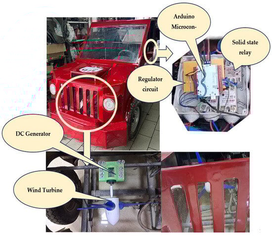
Figure 1.
The experimental setup of the EWV.
Figure 2 shows the detailed wiring diagram of the EWV control system components where it consists of a regulator circuit, switching circuit, Arduino mega microcontroller, two batteries, battery sensor and motor. The objective of the switching circuit is switching between the main battery and the backup battery according to Table 1. The switching circuit contains an array of relays to can on/off the charging of each battery. The regulator circuit contains a Zener diode and a series of capacitors to regulate the generated voltage. There are two modes, the first mode is the open loop mode without controller. The second mode is the closed loop where the proposed control techniques will be used to enhance dynamic performance.
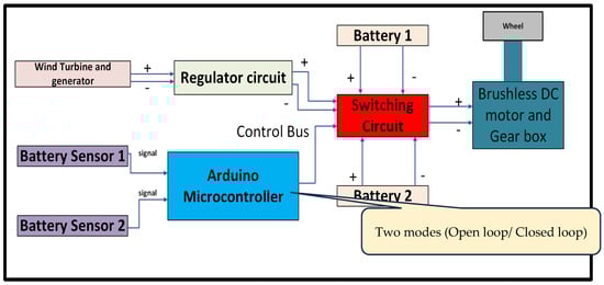
Figure 2.
EWV control unit block diagram.

Table 1.
Parameters of the nonlinear EV system.
Figure 3 represents a battery management system where two sensors monitor battery levels and determine which battery is active and which one is charging. When both batteries are nearly full, battery 1 (B1) is active and battery 2 (B2) is charging. If B1 is critically low, battery 2 (B2) takes over, and B1 starts charging. When B1 has a moderate charge but B2 is low, B1 remains active while B2 charges. If both batteries are low but B2 has slightly more charge, B2 is used while B1 charges. The system dynamically switches between the batteries to ensure continuous power supply and efficient charging.
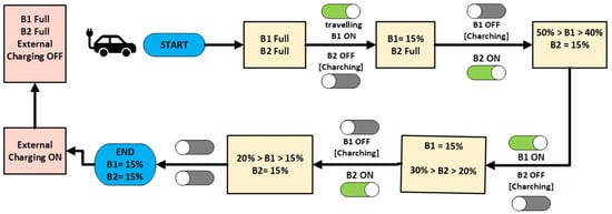
Figure 3.
The switching circuit sequence.
The simplified switching circuit block diagram is illustrated in Figure 4. This circuit is an Arduino-controlled wind energy management system that efficiently regulates power flow between a wind turbine, battery packs, and a motor driver using relays, contactors, and voltage sensors. The wind turbine generates power, which is managed by a charge controller and stored in battery packs. The Arduino Mega microcontroller monitors voltage levels via voltage sensors and controls relays to switch between power sources dynamically. Contactors handle high-power switching, while the motor driver operates a motor when sufficient energy is available. This setup ensures optimal power utilization, battery protection, and automatic switching based on energy availability.
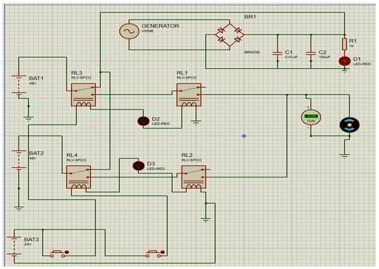
Figure 4.
The simplified switching circuit block diagram.
3. Mathematical Model and Validation
This section illustrates the nonlinear state space model of proposed EWV can be considered as follows.
where is the mass of the electric vehicle, is the gravity acceleration, the driving velocity of the vehicle, the rolling resistance coefficient, the air density, the frontal area of the vehicle, the drag coefficient and the hillclimbing angle, is considered the armature and field current, ω the angular speed of the motor, is the wheel radius. is the gear ratio. La the armature inductance, the armature resistance, the field winding inductance, the field winding resistance, the mutual inductance among the field and armature windings, B the viscous coefficient, the moment of inertia of the motor, the external torque and the input voltage.
Table 1 describes the EV parameters and specifications.
A comparison between the response of the proposed model state space and the EWV experimental setup response. The result of this comparison is demonstrated in Figure 5. It can be noted that the proposed model simulates significantly the EV experimental setup, but the response of EV experimental setup suffers from high noise due to the system uncertainty and nonlinearity.
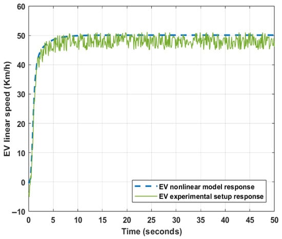
Figure 5.
The EWV linear open loop speed response.
4. Wind Turbine Power Estimation
This section illustrates the effect of changing the swept area of the wind turbine and the EWV travelling speed on the generated power. So, Figure 6 displays the generated wind power at various EWV speeds and 0.5 m2 swept area. It should be remembered that as speed increases, more power will be produced and charging time will decrease.
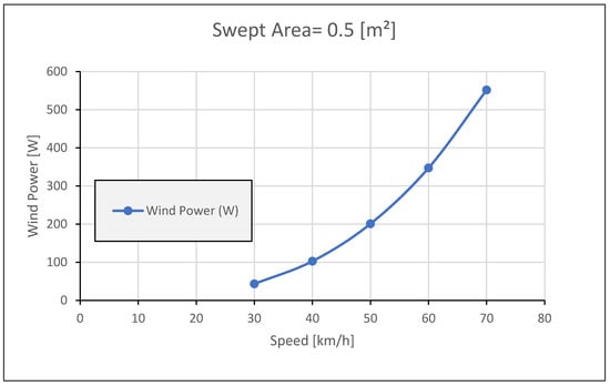
Figure 6.
Wind Power vs. Vehicle Speed at 0.5 [m2] Swept Area.
Figure 7 demonstrates the generated wind power for swept area 0.7 m2. The generated power will be increased at the same charging time compared to the swept area 0.5 m2.
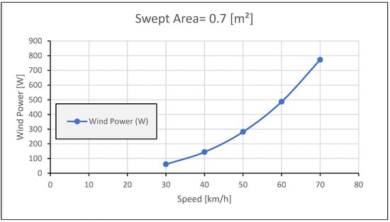
Figure 7.
Wind Power vs. Vehicle Speed at 0.7 [m2] Swept Area.
Also, in Figure 8 the power generated will be increased significantly at swept area 1 m2 compared to swept area 0.5 m2 and 0.7 m2.
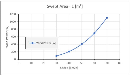
Figure 8.
Wind Power vs. Vehicle Speed at 1 [m2] Swept Area.
In Figure 9, it can be noted that the difference between the generated power at swept area 1 m2 and 1.2 m2 is not high. So, in this paper the designed swept area is 0.7 m2 to compromise between the generated power and the drag force losses.
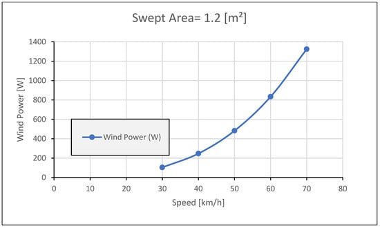
Figure 9.
Wind Power vs. Vehicle Speed at 1.2 [m2] Swept Area.
Figure 10 displays the generated power at several swept areas. These results confirm the feasibility of enhancing vehicle performance using wind-based auxiliary charging systems.
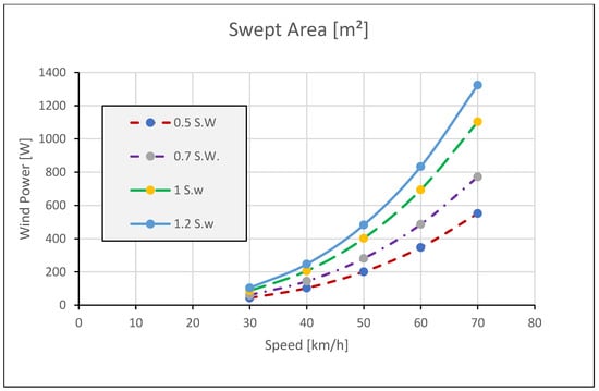
Figure 10.
Wind Power vs. Vehicle Speed at different Swept Area.
The fan blades were manufactured from light material (PVC) which can be sensitive to wind motion. Also, the designed swept area is 0.7 m2 to compromise between the generated power and the drag force losses. The wind turbine is considered a second source for the EWV charge which helps the battery to save its energy and makes the EWV travel more distances. The electric vehicle was designed to travel with two passengers. But the test performed with one passenger has a weight of 75 kg. The test was executed through highway road without traffic to adjust the vehicle at a certain average speed and the road has zero inclination approximately.
5. Wind Turbine Efficiency
Adding wind turbines beneath the front bumper is a new approach to using renewable energy. As it drives forward, the EWV encounters air resistance. Power is generated when the air mass’s resistance strikes turbine blades. A battery stores the generated energy before it is used in the motor. As a result, less fuel is used to produce energy, lowering the cost. Depending on the wind speed and the diameter of the revolving blades, wind turbines produce electricity. An eight-fold boost in power generation is achieved when wind speeds double. Therefore, more power could be produced than with a conventional wind turbine at the same wind speed by changing the fluid dynamic character of the wind near the blades. Additionally, power generation can start at much lower wind speeds, increasing the number of possible locations for wind power production.
The objective is to increase the traveling period and save power. The following section demonstrates the EWV performance and the battery capacity through the traveling period.
Assume ideal wind power (before losses):
- : Air density (typically 1.225 kg/m3)
- : Turbine swept area (in m2).
- : Relative wind speed (≈vehicle speed if mounted frontally)
Accounting for Losses by applying three efficiency terms:
- Aerodynamic efficiency (also includes Betz limit, max ≈59%, typical ~30–45%)
- Mechanical efficiency of the drivetrain and bearings (typically 80–90%)
- Electrical efficiency of the generator and rectifier (typically 85–95%)
Real Output Power to Battery B:
Total wind turbine efficiency:
Backup Battery Charging Model (with Losses)
If is the power delivered after losses, and is charge controller efficiency:
Battery voltage over time
The switching circuit equation
Output power to the EV load
where is the Voltage of the main battery at time t. is the Voltage of the backup battery at time t. is the Voltage threshold for switching between batteries. is the capacitance equivalent of Battery B (capacity). is the charge stored in Battery B at time t. S(t) is the switching function (1 for Battery A, 0 for B). is the supply voltage to EV load. is the current drawn by the EV from the selected battery. is the power required by the EV motor at time t.
6. Wind Turbine Validation
The EWV system was established with a system that involves a twin battery configuration, Battery 1 and Battery 2, both of which are initially fully charged and regulated by a switching circuit utilized with a wind turbine. The wind turbine corresponds to both batteries and is tasked with charging them according to the system’s energy requirements. The system functions cyclically, dynamically alternating between Battery 1 and Battery 2 according to their charge levels. The wind turbine is essential in charging the batteries, directing its output to the battery with the lower charge at any moment. The switching mechanism maintains balanced charge levels in the batteries, preventing one from becoming severely reduced while the other is overloaded. Technology efficiently harnesses the energy generated by the wind turbine to ensure a consistent energy supply while optimizing the charging process’s efficiency. The switching circuit mitigates the excessive discharge of a single battery and guarantees the efficient utilization of the energy storage capacity of both batteries.
In this section, The EWV will be operated in manual mode (without control). To find the required battery capacity to operate a motor rated at 48 V and 12 A for 3 h.
Capacity (Ah) = Current (A) × Time (h)
Capacity = 12 A × 3 h = 36 Ah
Energy (Wh) = Voltage × Capacity = 48 × 36 = 1728 Wh
Time (hours) = Generator Power (W)/Battery Energy (Wh)
Time = 200/1728 = 8.64 h
Table 2 shows the recorded practical test of the EWV without using the switching circuit. It can be noted that the time of traveling is 2 h. only due to the drag force losses. But, using the wind turbine 15.25% of battery capacity was saved. Also, Figure 11 demonstrates the relation between the battery capacity and with time for each case.
Table 2.
EWV traveling performance with one battery.
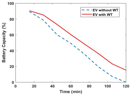
Figure 11.
EV with and without WT (one battery).
Table 3 shows the EWV performance through using two batteries. It can be noted that the system with wind turbine can save 18.21% of battery 1 capacity and save 45.43% of battery 2 capacity. Also, Figure 6 illustrates the battery discharging history with and without wind turbine. Figure 12 displays the relation between the battery capacity and with time for each scenario.
Table 3.
EWV traveling performance with two batteries.
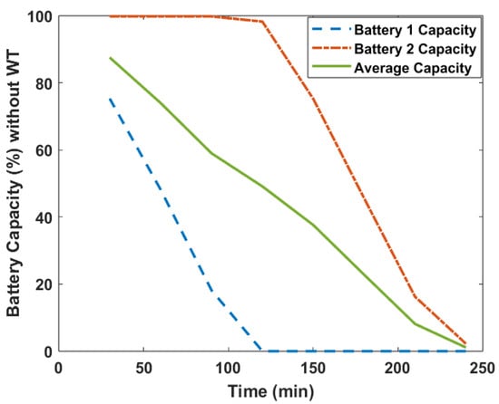
Figure 12.
EV with and without WT (two batteries).
7. Modified Sliding Mode Control
Sliding mode control (SMC) has been used in several effective applications. For instance, power electronics and electrical drives are where the SMC is most useful. Two steps are required to finish the controller design for the sliding mode control. For the sliding motion to attain the necessary performance, the first stage involves designing a sliding surface. The selection of a control law that will make the transferring surface appealing to the system state is the focus of the second stage.
From a practical point of view SMC permits for controlling nonlinear processes subject to external disturbances and heavy model uncertainties.
Assume the nonlinear SISO system.
where and stand for the scalar output and input variable, and represents the state vector. SMC combines two phases.
The first phase is sliding surface design. The second phase is the control input design. The first phase is the description of a certain scalar function of the system state, says Usually, the sliding surface depends on the tracking error together with a certain number of its derivatives.
The closed loop system can be implemented as demonstrated in the following block diagram Figure 13. It can be noted that the system was exposed to two external disturbances. The first disturbance is the road torque which depends on the road slope angle. The second disturbance is the road speed profile which will be changed continuously.
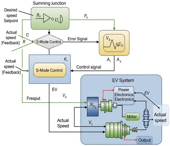
Figure 13.
The overall closed loop system block scheme (second mode of EWV).
It is known that the standard (or first-order) sliding mode control, the control is discontinuous across the manifold .
Assume that the sliding mode surface depends on just a single scalar parameter, p. The selection of the positive parameter p is almost arbitrary according to the requirements of the designer.
Most studies believe that the sgn function is the primary cause of chattering in the control signal of sliding mode strategy; nevertheless, this study shows that chattering in the control signal will occur when the value of is constant. The suggested method eliminates chattering, increases flexibility, improves robustness, and is insensitive to system uncertainty by using the single neuron PID (SNPID) methodology to adjust the value of online. The effect of modification on the form of the control signal is seen in Figure 14.
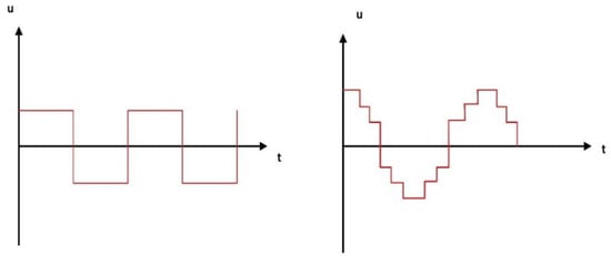
Figure 14.
Control signal at constant value of (left) and control signal at continuous change in value (right).
To enhance the robustness and adaptability of the SNPID controller, the fuzzy logic used to design update the neuron weights online instead of the conventional learning methods. The learning rates are critical parameters in SNPID design. In the normal SNPID, it is fixed, and the weighted coefficients will increase or decrease in the same proportion to enhance the performances of the controller, the fuzzy logic employed to dynamically adjust the proportional, integral and derivative learning rates. So, the proposed control considers a hybrid technique which combines between the sliding mode control and the SNPID updated with fuzzy logic. The proposed control technique can be called the modified sliding mode control which demonstrated in Figure 15.
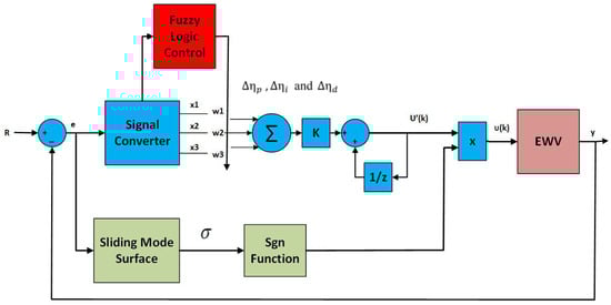
Figure 15.
The modified sliding mode control.
The weights-learning algorithms of this method are non-supervised Hebb learning rules as shown in Equation (23) and the adjustment of the learning rate are presented: as follows:
where Δηp(k), Δηi (k) and ΔηD(k) are the outputs of the fuzzy controller.
To validate that the proposed fuzzy-aided sliding mode control strategy guarantees the existence of sliding motion, we analyze the system behavior near the switching surface
Let the sliding surface be defined as
here is the tracking error, and are weighting constants. The discrete control law in Figure 15 can be expressed as:
where the weights are adaptively tuned using the fuzzy logic controller based on are signal converter outputs derived from error dynamics.
We define a Lyapunov candidate:
Taking the time difference (for discrete-time system):
To ensure convergence, we must show:
Substituting the control law and assuming is designed such that:
then:
which confirms that the trajectories will reach the sliding surface in finite time, hence satisfying the reachability condition.
The use of fuzzy logic enhances this design by dynamically adjusting the controller gains based on the real-time system behavior, ensuring that the gain K is sufficiently large near the surface while preventing excessive chattering.
To assess the impact of fuzzy logic integration on the overall response speed of the control system, we conducted a numerical benchmark by measuring the execution time of the fuzzy inference engine within the control loop. The average execution time per iteration was found to be 10 ms which is negligible compared to the total sampling interval of 100 ms. This indicates that the fuzzy logic controller (FLC) does not introduce significant delay or computational load. Additionally, the control system was tested under real-time conditions using MATLAB/Simulink Real-Time with Arduino microcontroller, confirming that the signal processing and decision-making remain within acceptable bounds for fast dynamic response.
Table 4, Table 5 and Table 6 present the fuzzy rules of this method. The membership function adopts triangle function; the fuzzy inference adopts Madami rules and the defuzzification adopts a weighted average method.
Table 4.
The Rule base of .
Table 5.
The Rule base of .
Table 6.
The Rule base of .
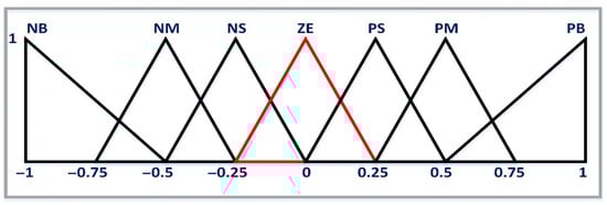
Figure 16.
Memberships function of inputs (e, ∆e).
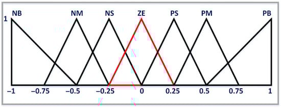
Figure 17.
Memberships functions of outputs (.
The adaptation law of depends on the SNPID strategy as demonstrated in Equation (31).
where is a proportional error, is an integral error and is a differential error.
There are several weights learning algorithms according to the learning theory of neural networks while the famous algorithm that used in this work is the supervised Hebb learning rule as follows.
where is the error, and are the proportion learning speed, the integral learning speed and the differential learning speed respectively. Also, are the initial values of neuron weights. There are several parameters for the proposed SMC-SNPID control technique that should be selected properly.
So, the harmony search optimization has been used to find the proper value for these parameters which are . The objective function used for this purpose is as follows Equation (37).
The actual closed-loop specification of the system with controller, rise time (), maximum overshoot (), settling time (), and steady state error (). This objective function can fulfill the designer requirement using the weighting factor value (β). The factor is set to be larger than 0.7 to reduce overshoot and steady-state error. If this factor is set smaller than 0.7 the rise time and settling time will be reduced.
8. Results and Desiccation
Figure 18 shows the EV linear velocity dynamic response at a fixed operating speed point. The objective is investigation the performance of the EV by applying a certain reference speed. It can be noted that the modified sliding mode control has a faster response, smooth behavior, no overshoot, and zero steady-state errors. The EV can reach the required speed in 35 s approximately.
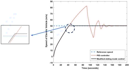
Figure 18.
The EV velocity response at fixed reference speed.
Various forms of standardized driving cycles are utilized all around the world. In this test, a famous speed profile cycle was applied to ensure the proposed control rigidity under several operation points. It can be noted that the proposed control can track the preselected profile as in Figure 19.
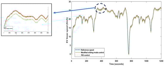
Figure 19.
The output response at variable speed profile.
9. Conclusions
A new wind energy harvesting technique is presented in this research to improve the performance of the electric-wind vehicle (EWV). An electric-wind vehicle model with a wind turbine on the front may harness wind that blows in the opposite direction of the vehicle it is driving. The generator turns on by turning wind energy into electrical power and storing it in a backup battery when the primary battery runs low. Depending on the battery’s capacity, a switching circuit was created to alternate between the primary and backup batteries. While the primary battery was discharging during the EWV’s journey, the backup battery was being charged via the wind turbine. The reference speed EWV is tracked by the modified sliding mode control, which controls the speed by alternating between the two batteries. The suggested approach was investigated using several scenarios. According to the findings, the suggested approach can save 30% more electricity than the traditional one. Additionally, compared to PID control, which provides subpar performance, the modified sliding mode control can improve the EWV dynamic performance.
Author Contributions
Conceptualization, M.A.S. and S.E.-k.; methodology, M.A.S. and S.E.-k.; software, M.A.S.; validation, M.A.S. and S.E.-k.; formal analysis, M.A.S. and S.E.-k.; investigation, M.A.S. and R.S.S.; resources, M.A.S. and S.E.-k.; data curation, M.A.S. and S.E.-k.; writing—original draft preparation; writing—review and editing, all; visualization, all; supervision, M.A.S. and S.E.-k.; project administration, M.A.S. and S.E.-k.; funding acquisition, M.A.S. and S.E.-k. All authors have read and agreed to the published version of the manuscript.
Funding
This research received no external funding.
Data Availability Statement
Data is contained within the article.
Conflicts of Interest
Ramy S. Soliman is employed by Valeo Company. The remaining authors declare that the research was conducted in the absence of any commercial or financial relationships that could be construed as a potential conflict of interest.
References
- Shamseldin, M.A. Adaptive Controller with PID, FOPID, and NPID Compensators for Tracking Control of Electric—Wind Vehicle Mohamed. J. Robot. Control 2022, 3, 546. [Google Scholar] [CrossRef]
- He, R.; Yan, Y.; Hu, D. Optimised adaptive control methodology for mode transition of hybrid electric vehicle based on the dynamic characteristics analysis. Veh. Syst. Dyn. 2021, 59, 1282–1303. [Google Scholar] [CrossRef]
- Nguefack, C.M.F.; Fotso, B.M.; Talawo, R.C.; Fogue, M. Aerodynamic Analysis of an Electric Vehicle Equipped with Horizontal Axis Savonius Wind Turbines. Int. J. Recent Trends Eng. Res. 2019, 5, 17–26. [Google Scholar] [CrossRef]
- Zhang, Y.; Wang, W.; Xiang, C.; Yang, C.; Peng, H.; Wei, C. A swarm intelligence-based predictive regenerative braking control strategy for hybrid electric vehicle. Veh. Syst. Dyn. 2022, 60, 973–997. [Google Scholar] [CrossRef]
- Shiravani, F.; Alkorta, P.; Cortajarena, J.A.; Barambones, O. An Enhanced Sliding Mode Speed Control for Induction Motor Drives. Actuators 2022, 11, 18. [Google Scholar] [CrossRef]
- Leach, F.; Kalghatgi, G.; Stone, R.; Miles, P. The scope for improving the efficiency and environmental impact of internal combustion engines. Transp. Eng. 2020, 1, 100005. [Google Scholar] [CrossRef]
- Chen, M.; Patel, R. The Future of Clean Energy Vehicles: Challenges and Opportunities. Renew. Energy Rev. 2019, 45, 987–995. [Google Scholar] [CrossRef]
- Xu, Y.; Zhang, B.; Kang, Y.; Wang, H. Cascaded Extended State Observer-Based Composite Sliding-Mode Controller for a PMSM Speed-Loop Anti-Interference Control Strategy. Sensors 2025, 25, 1133. [Google Scholar] [CrossRef]
- Junejo, A.K.; Xu, W.E.I.; Member, S.; Tang, Y.; Member, S.; Shahab, M. Novel Fast Terminal Reaching Law Based Composite Speed Control of PMSM Drive System. IEEE Access 2022, 10, 82202–82213. [Google Scholar] [CrossRef]
- Xu, W.; Junejo, A.K.; Liu, Y.; Hussien, M.G.; Zhu, J. Transactions on Power Electronics an Efficient Anti-Disturbance Sliding-Mode Speed Control Method for PMSM Drive Systems. IEEE Trans. Power Electron. 2020, 36, 6879–6891. [Google Scholar] [CrossRef]
- Du, G.; Xu, W.; Member, S.; Zhu, J.; Member, S. Effects of Design Parameters on the Multiphysics Performance of High-Speed Permanent Magnet Machines. IEEE Trans. Ind. Electron. 2019, 67, 3472–3483. [Google Scholar] [CrossRef]
- Shamseldin, M.A. An Efficient Single Neuron PID—Sliding Mode Tracking Control for Simple Electric Vehicle Model. J. Appl. Nonlinear Dyn. 2022, 11, 1–15. [Google Scholar] [CrossRef]
- Salem, F.B.; Derbel, N. Position control performance improvement of DTC-SVM for an induction motor: Application to photovoltaic panel position Electric Power Components and Systems Direct Torque Control of Induction Motors Based on Discrete Space Vector Modulation Using Adaptive Sliding Mode Control. Electr. Power Compon. Syst. 2014, 42, 1598–1610. [Google Scholar] [CrossRef]
- Xu, W.; Jiang, Y.; Mu, C.; Blaabjerg, F. Improved Nonlinear Flux Observer Based Second-Order SOIFO for PMSM Sensorless Control. IEEE Trans. Power Electron. 2019, 34, 565–579. [Google Scholar] [CrossRef]
- Yang, X.; Yu, J.; Wang, Q.; Zhao, L.; Yu, H.; Lin, C. Neurocomputing Adaptive fuzzy finite-time command filtered tracking control for permanent magnet synchronous motors. Neurocomputing 2019, 337, 110–119. [Google Scholar] [CrossRef]
- Parthasarathy, S.S.; Ferrão, P. ScienceDirect ScienceDirect A novel neural network intelligent for vector controlled Symposium controller induction motor drive Assessing the feasibility of using the heat demand-outdoor temperature function for a long-term district heat demand forecast. Energy Procedia 2017, 138, 692–697. [Google Scholar] [CrossRef]
- Ben Salem, F.; Almousa, M.T.; Derbel, N. Direct Torque Control with Space Vector Modulation (DTC-SVM) with Adaptive Fractional-Order Sliding Mode: A Path Towards Improved Electric Vehicle Propulsion. World Electr. Veh. J. 2024, 15, 563. [Google Scholar] [CrossRef]
- Mwasilu, F.; Jung, J. Enhanced Fault-Tolerant Control of Interior PMSMs Based on an Adaptive EKF for EV Traction Applications. IEEE Trans. Power Electron. 2016, 31, 5746–5758. [Google Scholar] [CrossRef]
- Mani, P.; Rajan, R.; Shanmugam, L.; Joo, Y.H. Adaptive fractional fuzzy integral sliding mode control for PMSM model. IEEE Trans. Fuzzy Syst. 2018, 8, 1674–1686. [Google Scholar] [CrossRef]
- Zhang, W.; Li, D.; Lou, X.; Xu, D. Prescribed Performance Adaptive Backstepping Control for Winding Segmented Permanent Magnet Linear Synchronous Motor. Math. Comput. Appl. 2020, 25, 18. [Google Scholar] [CrossRef]
- Salhi, B.; Benfdila, A. Recursive gain controller for strict feedback systems. Int. J. Control. 2021, 96, 711–718. [Google Scholar] [CrossRef]
- Ammar, A. Adaptive MRAC-based direct torque control with SVM for sensorless induction motor using adaptive observer. Int. J. Adv. Manuf. Technol. 2017, 91, 1631–1641. [Google Scholar] [CrossRef]
- Junejo, A.K.; Xu, W.; Member, S.; Mu, C.; Member, S. Adaptive Speed Control of PMSM Drive System Based a New Sliding-Mode Reaching Law. IEEE Trans. Power Electron. 2020, 35, 12110–12121. [Google Scholar] [CrossRef]
- Law, R.; Huang, C.; Wang, T.; Li, M.; Yu, Y. Applied sciences Sliding Mode Control of Servo Feed System Based on Fuzzy. Law. Appl. Sci. 2023, 13, 6086. [Google Scholar]
- He, J.; Tang, R.; Wu, Q.; Zhang, C.; Wu, G.; Huang, S. Robust predictive current control of permanent magnet synchronous motor using voltage coefficient matrix update. Int. J. Electr. Power Energy Syst. 2024, 159, 109999. [Google Scholar] [CrossRef]
- Yang, D.; Lu, H.; Zhang, C. Research on Improved Current Predictive Control of Permanent Magnet Synchronous Motor Research on Improved Current Predictive Control of Permanent Magnet Synchronous Motor. J. Phys. Conf. Ser. 2022, 2206, 012005. [Google Scholar] [CrossRef]
- Lee, J.-Y.; Lee, J.-S. An Improved Zero-Current Distortion Compensation Method for the Soft-Start of the Vienna Rectifier. Electronics 2024, 13, 1806. [Google Scholar] [CrossRef]
- Mohamed Ghany, M.A.A.; Shamseldin, M.A.; Ghany, A.M.A. A novel fuzzy self tuning technique of single neuron PID controller for brushless DC motor. Int. J. Power Electron. Drive Syst. 2017, 8, 1705–1713. [Google Scholar] [CrossRef][Green Version]
- Liu, P.; Chu, H.; Zheng, B. Robust sliding mode controller design of memristive Chua’s circuit systems. AIP Adv. 2022, 12, 025207. [Google Scholar] [CrossRef]
- Argha, A.; Li, L.; Su, S.W.; Nguyen, H. On LMI-based sliding mode control for uncertain discrete-time systems. J. Frankl. Inst. 2007, 353, 3857–3875. [Google Scholar] [CrossRef]
- Zhang, L.; Xia, Y.; Zhang, W.; Yang, W. Applied sciences Adaptive Command-Filtered Fuzzy Nonsingular Terminal Sliding Mode Backstepping Control for Linear Induction Motor. Appl. Sci. 2020, 10, 7405. [Google Scholar] [CrossRef]
- Zhu, W.; Chen, D.; Du, H.; Wang, X. Position control for permanent magnet synchronous motor based on neural network and terminal sliding mode control. Trans. Inst. Meas. Control. 2020, 42, 1632–1640. [Google Scholar] [CrossRef]


Disclaimer/Publisher’s Note: The statements, opinions and data contained in all publications are solely those of the individual author(s) and contributor(s) and not of MDPI and/or the editor(s). MDPI and/or the editor(s) disclaim responsibility for any injury to people or property resulting from any ideas, methods, instructions or products referred to in the content. |
© 2025 by the authors. Licensee MDPI, Basel, Switzerland. This article is an open access article distributed under the terms and conditions of the Creative Commons Attribution (CC BY) license (https://creativecommons.org/licenses/by/4.0/).