New Approach for Detecting Variability in Industrial Assembly Line Balancing Based on Multi-Criteria Analysis

Abstract

This paper focuses on the complex dynamics that concern assembly line balance in the context of mass customization within manufacturing. In fact, the increase in demand for customized products has heightened the complexities associated with achieving optimal efficiency, productivity, product quality, and customer satisfaction. The research proposes a multi-criteria analysis of statistical methods to determine the fluctuation of parameters affecting the state of balance of an assembly line. A 3D matrix model is suggested to analyze the parameters managing the assembly line. This representation is executed using the MATLAB R2024b tool, and a methodology for finding the variability of parameters affecting balance through statistical approaches is proposed. We observed that changes in parameters such as task times, worker efficiency, or material flow led to significant changes in the line’s overall balance. As a result, static balancing becomes inadequate to deal with the complexities introduced by these highly variable parameters. The novelty of this paper consists of the innovative integration of multi-criteria statistical analysis and 3D matrix modeling to detect parameter variability and optimize assembly line balancing. Conventional static approaches are often unable to capture the process-dynamic aspect of modern manufacturing. This work presents a systematic methodology capable of identifying, quantifying, and moderating the variability of key operating parameters. This methodology, carried out using MATLAB-based simulations, is based on principal component analysis (PCA) and correlation analysis to detect critical factors influencing balancing efficiency. By structuring assembly line parameters in a 3D matrix representation, this research gives a holistic, data-based method for improving decision-making in balancing procedures. The research goes beyond theoretical modeling by applying the approach to a real automotive assembly line, validating its effectiveness and demonstrating its practical applicability in industrial conditions.

1. Introduction

The manufacturing sector is undergoing a major transformation due to changing market requirements and technological advances. Assembly processes are one of the main trends in production today. They respond to different product specifications and changing demand volumes [1]. To compete in this increasingly digital and highly dynamic environment, companies need to anticipate, adapt, and respond effectively to changes in the global marketplace [2]. Mass customization is key to meeting the diverse and customized preferences of today’s consumers. Shorter product life cycles, greater production flexibility, and customized product configurations are some of the features [3]. On the contrary, assembly lines are used heavily to meet customer demand and adapt to product complexity in a competitive market [4]. Assembly line balance is one of the most important approaches to implementing harmonious production to optimize operator idle time and increase productivity [5]. The assembly line, where one worker completes a task at a station followed by another worker, and subsequently a conveyor belt, is a prevalent production process in the contemporary industrial manufacturing of identical products. Balancing production lines consists of assigning activities to workstations in order to optimize one or several objective functions [6].

In modern manufacturing, the assembly line balance problem (ALBP) is one of the most challenging problems as it involves allocating tasks to sequentially linked stations while taking priority connections into account [7]. Furthermore, dynamic rebalancing techniques can assist in sustaining a stable production process [8]. Identifying the key variables that significantly influence productivity is essential before implementing new balancing procedures. Such parameters may include operator skill levels [9], feeder line variability [10,11] and other variables that could have an impact on manufacturing line variability.

This present study examines the interaction between various parameters, using statistical methods to determine how variations in these parameters influence the balance of an assembly line [12]. The focus of this study is to examine the impact of variability on the balancing process of assembly lines [13]. Researchers have extensively examined the parameters that influence the balancing of variability in various systems within the scientific literature [14,15,16]. Figure 1 has been incorporated to visually represent the parameters and their influence on assembly line balancing. The key parameters identified in the scientific literature are shown in this figure in a systematic overview, categorized according to their direct impact on overall balancing performance. To do this, we structure these parameters in an arborescent manner, allowing researchers to better understand the underlying factors of balancing variability, whilst also allowing for the identification of optimization and control scenarios to improve efficiency.

Figure 1. Parameters that can impact the balance of an assembly line.

The research focuses on a better insight into the influence of the high variability of these parameters on the overall balance of the system, thus contributing to the development of more efficient balancing techniques and improved performance. The use of statistical methods in industrial applications has been met with considerable interest, guaranteeing significant results. The main objective is to identify parameters with high variability that cause a dynamic balancing situation. Multi-criteria analysis with a radar graph was used to evaluate and select the right statistical methods which can be used to identify these parameters.

Despite numerous advances, existing approaches to analyzing variability in line balancing have several limitations. On the one hand, they often focus on aggregate performance indicators (averages, overall equipment effectiveness) without precisely identifying the most influential parameters; on the other hand, few studies incorporate a multi-criteria analysis of variability by parameter, combining statistical dispersion and relative importance in a systematic framework which limits understanding of the effects of variations on overall balance. Finally, work on fuzzy balancing makes it possible to model overall uncertainty but does not provide an operational diagnosis of specific variability factors, making targeted intervention difficult.

In this context, this article makes the following three main contributions:

• A generalizable approach for detecting, upstream, the critical parameters with high variability that cause imbalances, regardless of how the problem is formulated (SALBP-1, SALBP-2, SALBP-E, etc.);
• A multi-criteria analysis of appropriate statistical methods, including standard deviation, coefficient of variation, and significance tests, to select the most appropriate method for each parameter; this approach makes it possible to more effectively detect highly variable variables that impact production line balancing;
• A pragmatic illustration using the case study of automotive pre-assembly, demonstrating the measurable impact of the methodology (an average efficiency gain of 12% and a significant reduction in bottlenecks) and highlighting the potential for transferring it to other types of assembly lines under conditions of uncertainty.

The results of this study help to optimize assembly line performance, thus promoting greater efficiency and productivity. To achieve this it is essential to identify these key parameters in order to determine which factors require continuous monitoring and precise control. This research makes it easier to effectively parameterize assembly lines by explaining the causes that lead to changes in balance. To solve this problem, this paper explores the use of multi-criteria analysis of statistical methods, and a procedure for identifying the variability of parameters impacting balancing are proposed. In Section 2, a state-of-the-art review to position our study with a formal description of the problem is first provided. A preliminary knowledge review and a comprehensive review of existing statistical methods is carried out to justify the selection of the chosen methodology in Section 3. Section 4 presents a methodology for assessing the variability of balancing. The study presented in Section 5 evaluates the practicability of the suggested approach. The concluding Section 6 presents and analyses the results.

2. Related Work

2.1. Variability in Assembly Line Balancing

Assembly line balancing involves distributing tasks among workstations to ensure equal cycle times. Traditionally, these methods assume a deterministic environment (all parameters are known and fixed) and optimize simple criteria (number of workstations and cycle time). However, increased competition and customization (product variety and rapidly changing markets) are forcing companies to manage uncertainty and process variability.

2.1.1. Simulation Approaches and Industry 4.0

Numerical simulation is widely used to study variability in balancing. For example, the studies propose a three-step algorithm combining a mathematical model and a simulation of stochastic parameters [17]. They first balance the line deterministically, then ‘simulate’ the effect of parameter variability (part arrival, processing time, operator speed, etc.), and finally use a stochastic solver (OptQuest, OptTek Systems, Inc., Boulder, CO, USA) to adjust the control variables and maintain the desired cycle time despite the randomness [17]. This approach made it possible to maintain the target cycle time in the presence of variability, demonstrating that such an MIP + simulation coupling is effective in detecting the impact of random parameters on balancing. In general, several studies recommend using simulation (and sometimes stochastic optimization) to test different scenarios and validate the robustness of the calculated balances. A notable example of Industry 4.0 technologies is the use of digital twins. This study show that integrating a real-time virtual model, fed by sensor data, can improve overall productivity and mitigate the effects of disruptions [18]. Thus, continuous simulation coupled with real data acquisition enhances the ability to manage operational variability.

2.1.2. Traditional and Deterministic Approaches

Several recent studies highlight that traditional models neglect these dynamic aspects. Most balancing studies assume a static context with no variability (e.g., traditional ALBP objectives). The studies note that most models optimize capacity (minimizing the number of jobs given a cycle time) or vice versa, assuming deterministic operation times [19]. These models do not take into account real-world uncertainties (time overruns, breakdowns, and necessary reallocations) and lack robustness in the face of disruptions. Nor do they capture the impact of frequent changes (new products and variants) nor the intrinsic flexibility of systems.

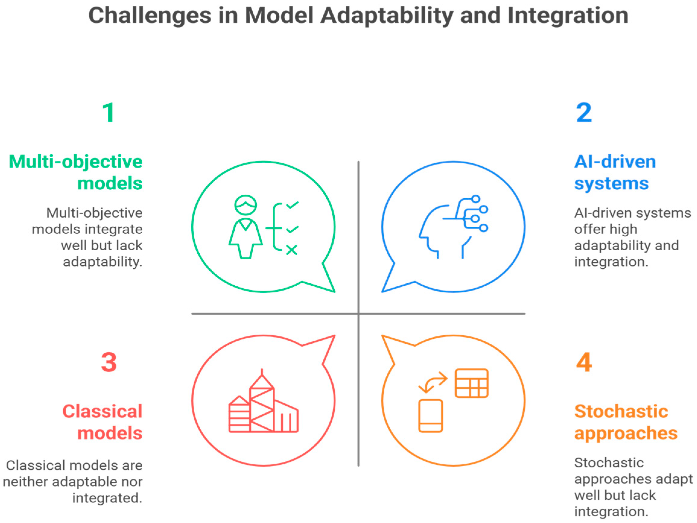
2.1.3. Robust and Stochastic Approaches

To manage uncertainty, robust or stochastic optimization methods have been developed. For example, the use of optimization under uncertainty (‘robust’) for line balancing, introducing the concept of stability and protection of solutions against variations [19]. Similarly, researchers proposed robust Mixed Integer Linear Programming models where task times are described by intervals or distributions, and where the objective is to minimize the number of positions while satisfying a performance level under the worst-case scenario [20]. These robust methods explicitly incorporate variability into the formulation (e.g., as additional constraints) but often remain focused on a ‘worst-case scenario’ or fixed scenarios. Their optimization is generally carried out before production, without the possibility of reallocation during operation. Others note that planning under uncertainty relies on these techniques, but that the emergence of multiple criteria (costs, flexibility, etc.) and decision support systems remains to be explored in greater depth.

2.1.4. Flexibility, Adaptability, and Artificial Intelligence

With the rise in AI and machine learning, other approaches are pushing the boundaries of adaptability. Recent studies propose a framework based on ‘intelligent’ rebalancing using Deep Reinforcement Learning coupled with high-fidelity simulation. This work takes into account dynamic factors that are often ignored (machine degradation, maintenance planning, operator learning/forgetting curves, etc.) in real time [20]. The results show that such a system can automatically adjust task allocation according to the current state (machine health and operator skill) and maintain production efficiency even when conditions change [20]. Other similar studies incorporate multi-agent algorithms or machine learning to anticipate and respond to disruptions, foreshadowing reconfigurable and ‘autonomous’ lines.

Recent research increasingly incorporates multi-objective flexibility and dynamic adaptability. Some studies explicitly introduce the concepts of flexibility and changeability into balancing: they consider several objectives (cost, system flexibility, and rebalancing time) and generate a Pareto front of adaptable equilibria under different future demand assumptions [21]. They find that traditional methods cannot dynamically reallocate tasks or scale the intrinsic flexibility of the line, which limits their relevance in uncertain contexts.

2.1.5. Fuzzy Methods Applied to Assembly Line Balancing

Fuzzy logic has been introduced into the field of ALB to explicitly model the uncertainties inherent in production systems. Rather than assuming strictly deterministic task durations (or assigning them known probability laws), the fuzzy approach represents these parameters by fuzzy numbers (e.g., triangular), with membership functions that reflect a degree of possibility for each possible value [22]. Thus, a task duration can be defined not as a single constant (e.g., 10 min) but as a range of ‘probable’ values with a central core (e.g., [8,10,12] minutes for a fuzzy triangle). This modeling uses possibility functions to replace probability distributions with possibility distributions [22]. In other words, fuzzy logic makes it possible to take into account the ambiguity surrounding processing times and line speed (cycle time) by encapsulating the uncertainty inherent in these variables rather than arbitrarily fixing them [23].

Several recognized research studies have applied these principles to improve the consideration of uncertainty in ALB. A study proposed a balancing method based on classical heuristics (such as COMSOAL) adapted to the fuzzy context [23]. Their results showed that balancing algorithms incorporating fuzzy times could provide solutions of equivalent or even superior quality to those obtained by traditional probabilistic or deterministic methods. In addition, other researchers studied the case of multiple model lines under uncertain task times, formulating a mixed balancing problem with fuzzy variables. To do this, they had to transform the initial fuzzy model into an equivalent linear program and develop approximate fuzzy arithmetic operators, already highlighting the technical complexity involved in processing fuzzy numbers [23]. These initial studies confirmed the viability of the fuzzy approach for modeling random execution times in production while also highlighting the need for appropriate resolution methods.

Over the past decade, fuzzy models for ALB have multiplied and become more refined. For example, a study proposes a fuzzy extension of the classic SALBP-2 problem (single line balancing and cycle time criterion) by treating task times as triangular fuzzy numbers [24]. His approach is based on a multi-objective genetic algorithm that seeks to simultaneously minimize the fuzzy cycle time of the line and be a fuzzy work smoothing indicator (balanced load distribution). Other fuzzy criteria can also be considered. Another study proposed to extend this framework to straight and U-shaped lines with multiple objectives, such as maximizing the line efficiency (measured in a fuzzy manner) or minimizing the inactivity rate and the variability index of workstations, defined by fuzzy variables [24]. To do this, they use an adaptive genetic algorithm, combining self-adjustment rules and the Taguchi method to fine-tune the parameters, resulting in high-quality solutions on standard test benches [25]. At the same time, fuzzy logic has been applied to more complex variants of the balancing problem. For example, other authors have used fuzzy goal programming to address multiple goals with imprecise targets (such as an approximate number of positions or maximum cost), thus offering greater flexibility to decision-makers in the context of uncertain information [25]. More recently, a study of the worker assignment balancing problem introduced the Assembly Line Worker Assignment and Balancing Problem in a fuzzy environment. They were the first to explicitly model uncertainty about operator-dependent task durations using triangular fuzzy numbers, and to formulate a bi-objective genetic algorithm aimed at simultaneously minimizing the fuzzy cycle time of the line and its fuzzy smoothing index [22]. Their results highlighted the effect of the degree of vagueness of duration on the performance obtained and showed that such a fuzzy approach could improve the robustness of the solution with respect to fluctuations in operator performance. Fuzzy logic has also proven useful in the field of automated lines: a recent study used it in the case of robotic lines to capture the variability in operating times from one robot to another (due to different capacities or technical hazards) [26]. They formulated a fuzzy RALBP (Robotic ALB) where the production rate and load smoothing were optimized, taking into account uncertain task times modeled as fuzzy, and obtained a set of Pareto compromise solutions reflecting the trade-offs between throughput and operational costs using a robust genetic algorithm [26]. Finally, it should be noted that fuzzy logic has been combined with other modern considerations. For example, a fuzzy expert system was integrated to assess the ergonomic risks of workstations in parallel with balancing, in order to address both the imprecision of task times and the qualitative assessment of human factors that are difficult to quantify [22]. All of these recent works demonstrate the viability of the fuzzy approach for dealing with various forms of uncertainty in line balancing.

2.2. Limitations of Existing Methods

Figure 2 illustrates the main challenges encountered in the current approaches to the adaptability and integration of the models used for balancing industrial assembly lines.

Figure 2. The limitations of existing methods.

Our contribution addresses these shortcomings by proposing an integrated multi-criteria framework for detecting highly variable parameters. Specifically, we model the factors influencing equilibrium using a 3D matrix (Y_i, X_ij, and V_ijk) that hierarchically captures roots, sub-parameters, and values. On this basis, a multi-criteria analysis of statistical methods allows us to select the appropriate techniques (e.g., PCA, analysis of variance, control charts, etc.) to detect the components with the most marked variability.

• It uses a 3D structure to pinpoint the sources of variability in industrial process parameters.
• It combines several relevant criteria (noise sensitivity, data requirements, calculation speed, etc.) to select the most effective statistical methods in a given context.
• It provides a systematic process for prioritizing and detecting critical parameters that impact balance, where previous approaches often remained global or empirical.
• Ultimately, it improves the sensitivity of balancing to real variations and facilitates the dynamic adaptation of workstations. In this respect, our method brings real scientific added value by filling the gaps identified in the current literature and paving the way for more robust and flexible industrial applications.

Our proposed variability detection methodology is designed to be universally applicable across these ALB classifications. In other words, it functions independently of whether the balancing problem is of type SALBP-1, SALBP-2, or any other variant. The approach operates upstream of the actual line-balancing solution phase: it focuses on identifying critical input parameters (denoted X_ij in our model) whose fluctuations have a significant impact on the feasibility of achieving a valid balance. This pre-solution analysis isolates which task durations or related parameters are most sensitive, potentially disrupting feasibility, regardless of the specific ALB formulation or objective being considered. By performing this, the methodology provides valuable insights before any optimization or heuristic solver is applied, and its usefulness does not depend on the particular ALB type one eventually chooses to solve. To illustrate the approach in practice, we applied our framework in a case study conforming to a typical simple ALB scenario with a fixed number of workstations and a minimized cycle time objective. This scenario aligns with the SALBP-1 style assumptions used in our study’s context. We emphasize that this choice of application (described in Section 4) is primarily for demonstration purposes, reflecting a common setting in assembly line balancing. It does not imply that the methodology is limited to SALBP-2 problems. On the contrary, because our variability detection step is formulated independently of the solving phase, the same framework can be integrated before tackling any assembly line balancing formulation, be it SALBP-1, SALBP-2, or more a complex extension. In summary, the proposed methodology generalizes across different ALB problem types, providing an upfront analysis of variability-sensitive parameters, whilst the specific example given in the paper showcases its use under one representative set of ALB assumptions.

3. Preliminary

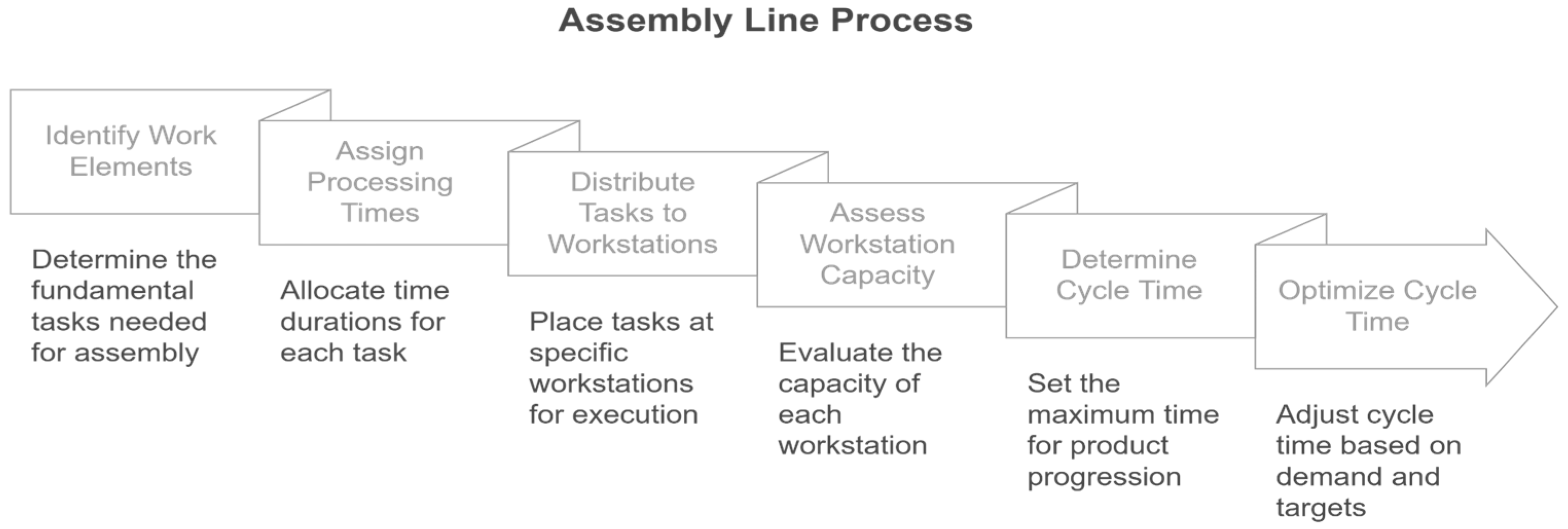
3.1. Assembly Line Balancing Problem

Assembly lines are used in modern industry to put together standardized items. The workstations on these lines are connected by a transport system, such as a conveyor belt, and the product is assembled from the first to the next [27].

The ALBP is particularly used in all industries where a product is manufactured by assembly production, such as automotive manufacturing, electronics, etc. [28]. Balancing an assembly line is a combinatorial optimization problem. It involves assigning operations to stations while respecting different constraints, so as to optimize the given efficiency criterion. This problem arises during the preliminary design of a new line, but also at the time of a major change in production. This requires effective task or work element allocation across the various workstations of an assembly line.

The SALBP problem consists of allocating a set of undivided tasks (subject to precedence constraints) to successive workstations in compliance with a given cycle time, by minimizing, for example, the number of workstations (SALBP-1) or, in reverse, for a fixed number of workstations minimizing the cycle time (SALBP-2). The standard models suppose the production of a single product (single-product line), a fixed operating time, and a paced transfer (paced line) [9].

This simplified model has given way to a large number of works. Various exact methods (notably branch-and-bound procedures) and heuristics (priority rules and taboo search-type metaheuristics or genetic algorithms) have been suggested and benchmarked over the past decades. Johnson’s seminal work or hybrid approaches such as Eureka have demonstrated the methodological depth of SALBP [29]. However, many of these studies are based on a simplified formulation.

The objective of the operation is to optimize this throughput under compliance with customer specifications. It is all about distributing work over all workstations, taking into account the fact that the load must be balanced in order to maximize production output and, implicitly, minimize waste due to bottlenecks that slow down the production flow [30]. Figure 3 shows the key components of the assembly line balancing.

Figure 3. Key components of the assembly line balancing.

The objectives of the ALBP are typically the following:

• Minimize the number of workstations required.
• Balance the workload as evenly as possible among the workstations.
• Ensure that the cycle time is not exceeded.
• Minimize production costs while meeting constraints.

ALBP resolution depends on several factors such as task priority, worker skills, and equipment limitations [31]. The elements of the assembly line are assigned to workstations in the most efficient manner possible. Many approaches can be used to solve ALBP, including heuristic methods, mathematical programming, and simulation techniques [32].

Researchers and practitioners often explore various strategies and algorithms to tackle the ALBP, making it an important area of study in operations research and production management. The fluctuation of parameters throughout the assembly line significantly affects its balance. This can lead to bottlenecks and missed production deadlines. In order to identify more precisely the parameters responsible for balancing variability, an approach based on statistical methods has been designed and implemented.

3.2. Statistical Methods in Production Line

The application of statistical analysis helps guarantee product quality and reliability, whilst also playing a key role in cost reduction and informed decision-making in production chains. We discuss the versatile utility of statistical methods in our economic sphere and perform an examination of their profound impact on manufacturing operations. To ensure higher industrial standards and facilitate product design, statistical methodologies are employed [33]. The adoption of statistical approaches in production management is not only good practice, but a fundamental necessity for companies wishing to remain competitive in a rapidly changing global economy [34].

• Quality improvement: Statistical Process Control (SPC) is one of the statistical methods used to monitor and control product quality. This involves the use of control charts to monitor key quality indicators in real time, enabling any deviation from desired standards to be identified immediately.
• Process optimization: Statistical methods using the Design of Experiments (DOE) approach to help identify key process parameters. Manufacturers can determine optimal settings that lead to higher yields, reduced resource costs, and minimized cycle times by dynamically adjusting and monitoring these parameters.
• Informed decision-making: Statistical data and analysis provides decision-makers with quantitative evidence to support their choices. Managers and engineers can make data-driven decisions to address production challenges, allocate resources effectively, and prioritize improvement projects based on a thorough understanding of the underlying factors.
• Continuous improvement: The concept is central to many production management methodologies, such as Lean and Six Sigma. Statistical methods, including root cause analysis, hypothesis testing, and process capability studies, help to identify the root causes of problems and develop solutions to prevent their recurrence. This results in ongoing enhancements to production processes.
• Compliance with standards: Statistical methods ensure that production processes adhere to quality and safety standards by maintaining meticulous records of processes and product characteristics. Organizations can demonstrate compliance with regulations and industry standards, which is particularly critical in highly regulated industries like pharmaceuticals and aerospace.
• Innovation and product development: Statistical methods are used during the research and development of the specifications of new products. They assist in assessing the performance and characteristics of prototypes and experimental designs. By quantifying the impact of various design variables, companies can develop innovative products that meet or exceed customer expectations.

The use of statistical techniques, analyses, and graphical representations is common in these articles to provide a comprehensive and rigorous account of the impact of statistical methods on production lines [35]. These applications of statistical methods are often discussed in detail, focusing on the methodologies employed, the data collected, and the results obtained as shown in Table 1 [36].

Table 1. The statistical methods used in production line.

Statistical Method	Description	Applications
Linear regression	Models the linear relationship between a dependent variable and one or more independent variables.	Predicting production yields, ensuring quality control, and optimizing resource allocation in manufacturing.
Logistic regression	Used to predict a binary outcome (yes/no) based on independent variables.	Identifying defective products, ensuring compliance with quality standards, and minimizing defects in production lines.
Analysis of variance (ANOVA)	Compares the means of three or more groups to determine if they are statistically different.	Assessing the impact of process parameters on product quality, optimizing production conditions, and enhancing overall process efficiency.
Multiple regression analysis	Extends linear regression to analyze the relationship between a dependent variable and multiple independent variables.	Predicting academic performance based on study time, diet, and sleep, etc.
Time-series analysis	Analyzes chronological data to identify trends, seasons, and patterns.	Predicting equipment failures, minimizing downtime, and optimizing maintenance schedules in production lines.
PCA	Reduces data dimensionality while preserving maximum variance.	Reducing the dimensionality of production data, facilitating data-driven decision-making, and improving overall process efficiency.
Cluster analysis	Groups similar observations into clusters based on similar characteristics.	Optimizing sub-processes within production lines, identifying bottlenecks, and enhancing resource allocation.
Artificial neural networks	A deep learning model inspired by the human brain’s functioning.	Process control, fault detection, and the optimization of complex production systems.
Survival analysis	Studies the time until a specific event, such as lifespan or time to failure.	Estimating equipment lifespans, optimizing maintenance schedules, and minimizing unplanned downtime.
Robust regression analysis	Identifies trends and relationships in data while minimizing the impact of outliers.	Modeling in the presence of noisy data, improving the accuracy of production predictions, and enhancing process robustness.

3.3. Multi-Criteria Analysis of Statistical Methods

The choice of which method to use should be based on the specific requirements of the problem to be solved [37]. Each statistical method is evaluated according to the following four selected criteria (complexity, robustness, modeling, and flexibility):

Complexity: The complexity parameter assesses the applicability and usability of methods. The complexity of a statistical method has a significant influence on its implementation.

Robustness: The measure of robustness of a statistical method and the ability to maintain acceptable performance even in the presence of atypical data or errors.

Modeling: Data modeling is key to obtaining accurate and reliable results from the chosen method, which is done by developing a model that ensures a clear representation of the data.

Flexibility: Flexibility refers to a statistical method’s ability to adapt to different situations or types of data.

Multi-criteria analysis shows that a number of key factors need to be taken into account when selecting the most effective statistical method as shown in Table 2.

Table 2. Multi-criteria analysis of statistical methods.

Statistical Method	Complexity	Robustness	Modeling	Flexibility	Applications
Linear regression	Low	Sensitive to outliers	Suitable for simple linear relationships	Limited	Linear prediction
Logistic regression	Moderate	Can handle imbalanced data	Binary variable prediction	Non-linear models possible	Binary classification
Analysis of variance (ANOVA)	Moderate	Sensitive to violations of assumptions	Comparison of means	Multiple factors and interactions possible	Multiple group comparisons
Multiple regression analysis	Moderate	Sensitive to outliers	Multiple linear models	Can include many independent variables	Prediction with multiple predictors
Time-series analysis	Moderate to high	Depends on time-series stability	Complex time-based models	Can handle non-linear time series	Time-series forecasting
PCA	Low to moderate	Sensitive to outliers	Dimensionality reduction	Used for data visualization and compression	Dimensionality reduction
Cluster analysis	Moderate to high	Can handle noisy data	Identification of similar groups	Variable number of clusters	Data segmentation
Artificial neural networks	High	Can learn from noisy data	Complex, non-linear modeling	Suitable for various machine learning problems	Machine learning and AI
Survival analysis	Moderate	Sensitive to censoring	Survival analysis	Parametric and non-parametric models	Survival studies
Robust regression analysis	Moderate	Resistant to outliers	Outlier-resistant linear modeling	Suitable for data with outliers	Robust modeling

A comparison of several statistical techniques is shown in Figure 4 by this radar chart based on the following six criteria: modeling, robustness, complexity, applications, flexibility, and a composite metric [38]. The numbers (1, 2, 3) indicate a qualitative scoring scale (1 = low, 2 = medium, 3 = high) used to visually represent the strengths and limitations of each method. This radar diagram shows that each method has its advantages and disadvantages, and the best approach must be determined by the particular requirements and how the different statistical approaches compare with each other for the analysis, including their robustness, adaptability, complexity and scope of application [39].

Figure 4. Graphical radar for statistical methods.

4. Methodology

The present study uses a multi-faceted approach to address the complexities of assembly line balance in the context of mass customization. A comprehensive statistical methods analysis is carried out to assess the variability of key parameters influencing assembly line stability. This entails creating a 3D matrix representation to analyze and visualize the piloting parameters. Employing the MATLAB tool, this matrix representation is subsequently utilized to simulate diverse scenarios and their effects on an assembly line. A procedure for identifying the variability of parameters impacting balancing leverages statistical methods to assess the influence of parameters such as task times, worker efficiency, and material flow. The methodology evaluates the impact of these parameters on the assembly line’s balance, productivity, and efficiency by adjusting them.

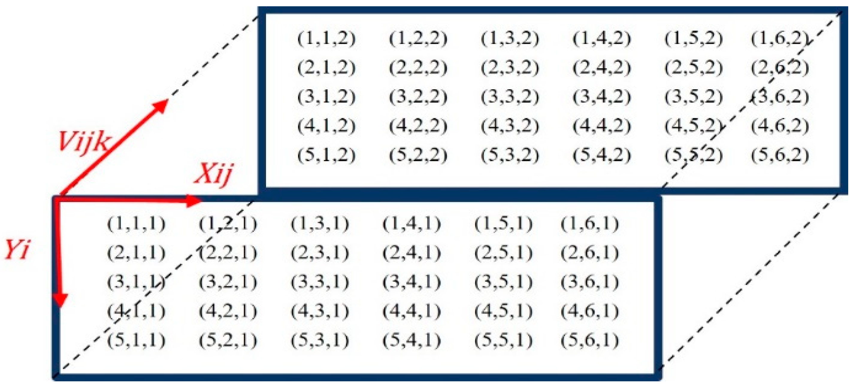
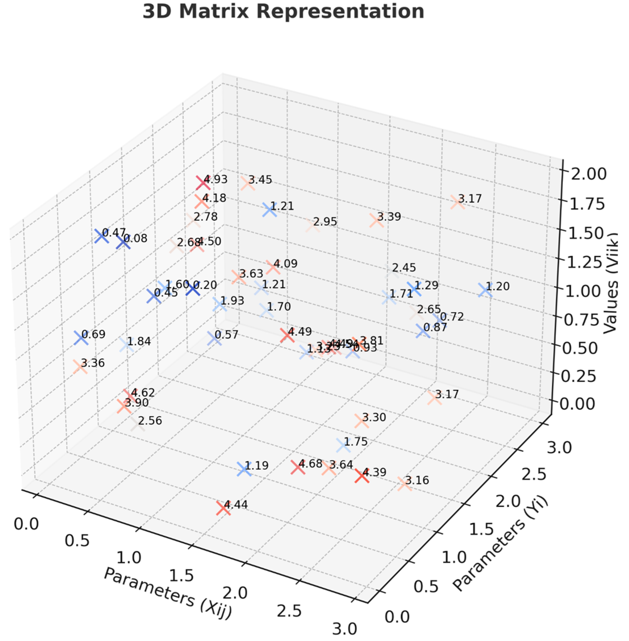
4.1. Matrix Representation

This research consists of constructing a model that identifies the principal factors of variability in the balancing process. To do this, we concentrate on the parameter Y, which characterizes the efficiency of manufacturing line balancing. Variability of parameters is arising from a set of contributing factors, labeled Y_i, each of which plays a distinct role to detect the overall variability in the balance of the production process. A structured representation is provided to clarify the interplay between Y (balancing efficiency) and Y_i (the key variables causing fluctuations), thereby offering insights into their interdependencies and highlighting potential strategies for optimization [40].

Figure 5 illustrates a hierarchical representation of the influence of parameter variations on assembly line balancing. In this diagram, X_ij denotes the j elemental factor contributing to the i high-level parameter Yi that affects overall balancing. In other words, each Y_i representing a specific source of variability, such as Takt time, workload, etc., is decomposed into several finer X_ij components whose fluctuations explain the variability of Y_i. At the same time, V_ijk represents a possible value (or a particular scenario) of parameter X_ij. The set of V_ijk values thus makes it possible to characterize the variability of each elementary factor and to analyze how these variations are reflected in the upper Y_i levels, and then in the overall Y balancing indicator [41].

Figure 5. A 3D matrix representation.

We used MATLAB (version R2024b) to carry out all the steps in our study. First was the modeling of the 3D matrix representing the interrelationships between tasks, scenarios, and stations; second, was applying statistical functions to quantify variability and then solving the assembly line balancing model. For balancing the line under constraints, we formulated a MILP model and used the optimization toolbox, employing the “intlinprog” function to solve binary and integer decision variables, as well as “linprog” for continuous sensitivity analyses. Next, for the statistical phase, we used the tools in the Statistics and Machine Learning Toolbox, in particular the “std()” function for standard deviation, “mad()” for dispersion, and “corr()” for correlation coefficients. This combination of MATLAB tools allowed us to automate the processing chain from 3D structure construction to statistical and operational optimization, whilst also ensuring rigorous reproducibility of our results.

To explain how the 3D matrix shown in the figure is constructed and used in the context of assembly line balancing, we need to understand the parameters of Y_i, X_ij, and V_ijk. To build a 3D matrix representation we use a mathematical model of the interaction of the overall parameters.

To construct the 3D matrix, consider the following steps:

❖

Define the dimensions:

• Let I be the number of root parameters Y_i.
• Let J_i be the number of sub-parameters X_ij for each Y_i.
• Let K_ij be the number of possible values V_ijk for each sub-parameter X_ij.

A can be represented with dimensions I × J × K, where A_ijk = V_ijk.

❖

Parameter descriptions:

• Y_i: These are the fundamental elements or factors that influence the overall variability in assembly line balancing, represented by Y.
• X_ij: These are sub-parameters or specific aspects that make up each root parameter Y_i.
• V_ijk: These represent the possible values that can take each sub-parameter X_ij.

❖

Matrix representation:

• Root rarameters (Y_i):
  • Y = {Y₁, Y₂ …, Y_I} are the main factors affecting the assembly line balancing.

• Sub-parameters (X_ij):
  • Each Y_i consists of several sub-parameters X_ij, where Y_i = {X_i1, X_i2 …, X_iJi}.

• Possible values (V_ijk):
  • Each X_ij has multiple possible values V_ijk, where X_ij = {V_ij1, V_ij2 …, V_ijKij}.

❖

The 3D matrix A:

The 3D matrix A is constructed as follows:

• For each i (corresponding to each Y_i);
• For each j (corresponding to each X_ij);
• For each k (corresponding to each V_ijk);

Then A_ijk = V_ijk.

This representation shows the links between the general parameter balancing Y, each decomposing factor Y_i, and their potential values (V_ijk) taken by the parameters X_ij.

The 3D matrix representation gives us an insight about the state of each specific Y_i parameter influencing the balancing efficiency parameter Y.

This 3D framework ensures that certain V_ijk values remain constant, indicating that the corresponding X_ij parameters have no influence on the Y_i parameters and thus the general balancing parameter Y maintains stability. However, some V_ijk values exhibit significant variability, so the associated X_ij parameters strongly affect Y_i, and consequently have an impact on the overall balancing parameter Y. This situation will be demonstrated through the example presented in the following section.

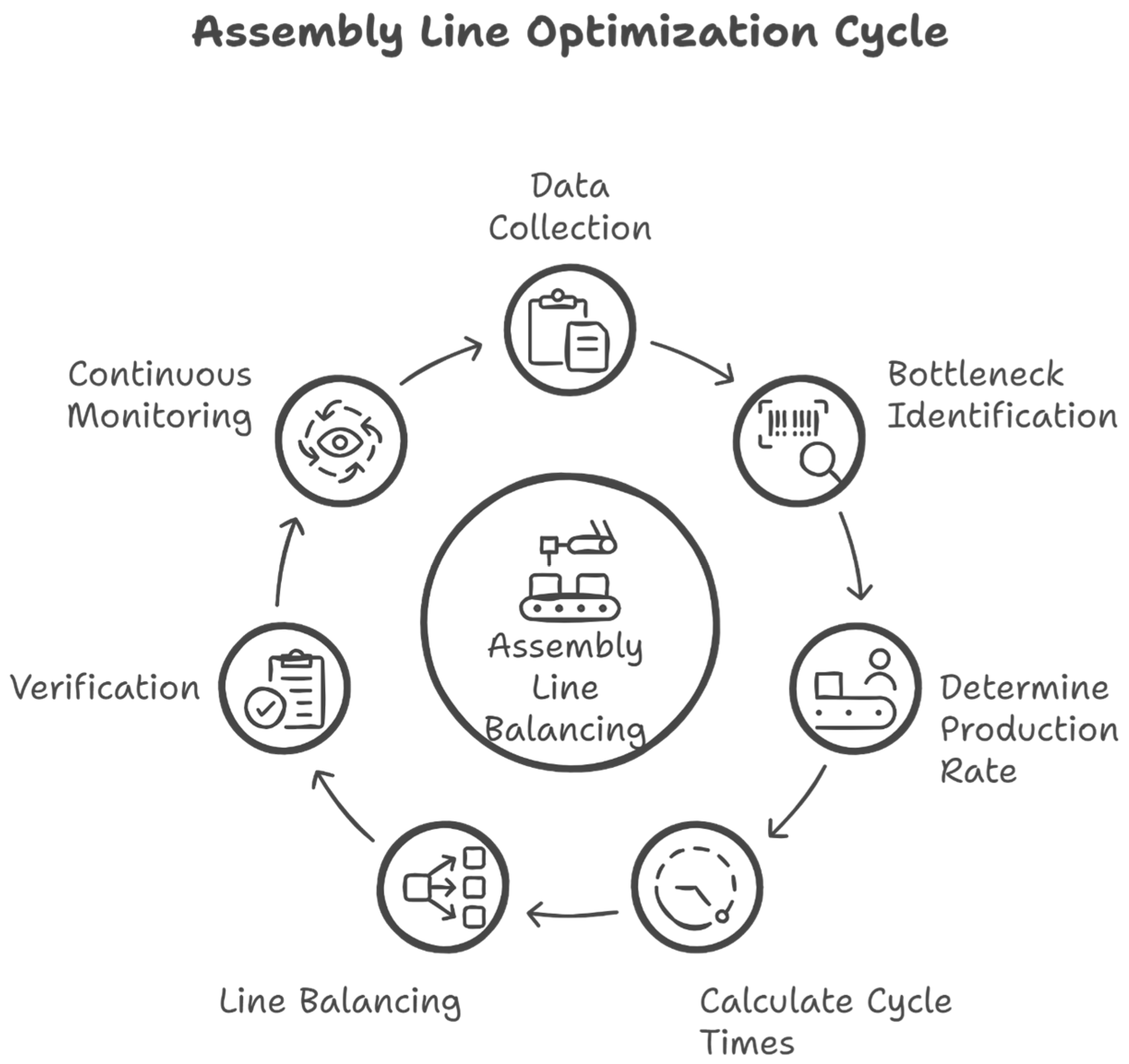
4.2. Procedure for Detecting Highly Variable Parameters Impacting Balancing

The objective is to implement the proposed methodology and achieve efficient balancing of the production line [40] by formalizing instructions and applying a 3D matrix and statistical techniques in MATLAB. The primary objective is to establish a uniform framework for detecting variability in assembly line balancing, building on prior work as shown in Figure 6 [42]. At the core of this methodology lies the 3D matrix, which operates as an intermediary between the overall efficiency indicator (Y) and the associated control parameters (Y_i and X_ij). The 3D matrix provides a better understanding of production line performance by examining in detail how different parameters influence the balance efficiency indicator. In particular, it highlights critical gaps in process performance. The value of 90% chosen as the balancing efficiency threshold is not arbitrary; it is based on recognized industry standards in Lean Manufacturing and in OEE assessments. Indeed, according to industry benchmarks, a balancing efficiency of over 90% is generally considered an acceptable level of performance for manual assembly lines [43]. In addition, we carried out a sensitivity analysis by varying this threshold to assess its impact, and the results obtained confirm the robustness of our choice of a 90% threshold [44].

Figure 6. New procedure for detecting parameters impacting balancing.

5. Case Study

In line with the previously described methodology, the next step involves its practical application in the automotive industry. To begin, we assembled a comprehensive dataset capturing the specific details of the manufacturing line used by the subject company. Notably, this company operates an assembly line featuring 29 manual stations, as illustrated in Figure 7.

Figure 7. Layout of the assembly line.

After an analysis of the database chosen in the automotive sector, and more precisely the wiring of automotive harnesses, we will follow the methodology proposed in the previous part.

The production line studied is dedicated to the pre-assembly of automotive wiring harnesses. Data collection took place over five consecutive weeks, with a single shift per day, recording a total of 7280 tasks. It comprises 29 manual workstations dedicated to cable routing, crimping, and quality control tasks. The variability observed during these operations was mainly due to differences in execution speed between operators, delays in material supply, and occasional tool reconfigurations [45].

5.1. Balancing the Assembly Line

The key steps to balancing an assembly line are as follows in Figure 8, and for more information see [46,47].

Figure 8. Static balancing procedure for a production line.

Our chrono analysis and variability study revealed that some stations were overburdened, leading to obstructions in the assembly process. Therefore, balancing the assembly line becomes necessary. The red horizontal line used as a reference in Figure 9 corresponds to the Takt time required to satisfy customer demand, i.e., the target production rate to be achieved. This is the cycle time threshold that each workstation must not exceed. If the cycle time of a station remains well below this threshold, the station is under-utilized, resulting in periods of inactivity (idle time) synonymous with wasted resources. Conversely, if the cycle time of a workstation exceeds this value, it becomes overloaded, creating a bottleneck which slows down the production flow and reduces the overall productivity of the assembly line. This visual cue makes it easy to identify load imbalances between stations (overload or under-utilization), so that the line can be rebalanced to ensure that each station operates as close as possible to the Takt time, without ever exceeding it. Figure 8 below provides a visual representation of this balance [48].

Figure 9. Variability study of the assembly line before balancing.

Through the utilization of one of the available balancing algorithms, as reported in the references [49,50,51], we have employed the greatest candidate rule algorithm to redistribute functions and operations across every station, hence optimizing the assembly line balance. Upon implementing the method, we analyzed the dynamic diagram of the workstations and determined that the line is now balanced, with all workstations displaying an equivalent task load, as illustrated in the graphic below.

By using the following Formula (1), we calculated the balancing efficiency indicator to properly measure the quality of balancing used:

$${\mathit{Y}}_{\mathit{b}}={\mathit{T}}_{\mathit{w}\mathit{c}}/(\mathit{m}\times {\mathit{T}}_{\mathit{s}})$$

(1)

where we note that

• Y_b: balancing efficiency indicator;
• T_wc: work content time;
• m: number of workstations;
• T_s: the duration of the slowest station.

Upon adopting the largest candidate rule algorithm [52], we determined that our line is optimally balanced, achieving a computed balancing efficiency indication of 97%. Through analysis of the assembly line’s variability, the Figure 10 below indicates that the line is considered balanced as the workload at each station seems to be balanced [53].

Figure 10. Variability study of the assembly line after balancing.

5.2. Matrix Representation

The database used contains a set of parameters Y_i that are automatically taken into account when regulating the studied production line.

Parameters Y_i and X_ij:

Y₁: Efficiency:

• X₁₁: Cadence: Number of conforming bundles made per time;
• X₁₂: Range time: Fixed index which expresses the duration of a cycle of assembly until the final control;
• X₁₃: Staff: number of staff present;
• X₁₄: Working hours.

Y₂: The time allocated to manufacture a beam:

• X₂₁: Shift time bottleneck;
• X₂₂: Shift time.

Y₃: Takt time:

• X₃₁: Production time;
• X₃₂: Daily demand.

Y₄: Product specification:

• X₄₁: Routing time;
• X₄₂: LAD frequency (product rotation frequency).

We used the MATLAB tool to convert the database into a 3D matrix composed of the parameters of Y_i and X_ij chosen in this example with the corresponding values V_ijk, as shown in Figure 11.

Figure 11. The 3D matrix application.

The parameters Y_i that have a significant impact on variability should be identified. Now we need to identify the parameter of Y_i which has a high degree of variability according to the 3D matrix shown in Figure 12.

Figure 12. Graphical representation of parameters Y_i.

It is clear from the graph that Y₁ (Efficiency) and Y₂ (The time required to construct a beam) have the highest degrees of variability.

5.3. Statistical Methods Application

5.3.1. Principal Component Analysis Application

The utilization of PCA enables the identification of parameters with high variability that impact assembly line balancing [54].

PCA is a technique that helps in reducing the dimensions of data while preserving most of the variance in the data [55]. In order to gain insight into the process we have been studying, it would be interesting to use PCA to see which parameters influence the variance of the efficiency of balancing Y in our study on assembly line balancing. We can also identify this through looking at the loadings or weights which are assigned to each of the variables on the various principal components. Furthermore, using this approach we can identify the parameters that have high variability and have a significant impact on assembly line balancing [56]. The implementation of PCA enables the identification of the parameters which have considerable variability, which influences the state of balance [57].

• Mathematical Model of PCA

❖

Standardization:

To ensure that each feature contributes equally to the analysis, the dataset is standardized [58]. Let X be the m × n data matrix, where m represents the number of observations and n denotes the number of features. The standardized data matrix Z is computed as follows:

$$\mathit{Z}={\displaystyle \frac{\mathit{X}-\mathit{\mu }}{\mathit{\sigma }}}$$

(2)

where μ and σ are the mean vector and the standard deviation vector of the features, respectively.

❖

Covariance matrix computation:

The next step involves computing the covariance matrix C of the standardized data matrix Z as follows:

$$\mathit{C}={\displaystyle \frac{1}{\mathit{m}-1}}{\mathit{Z}}^{\mathit{T}}\mathit{Z}$$

(3)

where the resulting covariance matrix C is an n × n symmetric matrix that captures the linear relationships between the features.

❖

Eigenvalues and eigenvectors:

Eigenvalues and eigenvectors of the covariance matrix C are then calculated as follows:

$$\mathit{C}{\mathit{v}}_{\mathit{i}}={\mathit{\lambda }}_{\mathit{i}}{\mathit{v}}_{\mathit{i}}$$

(4)

where λ_i represents the eigenvalue and v_i is the corresponding eigenvector.

❖

Principal components:

The eigenvalues λ_i are sorted in descending order, and the corresponding eigenvectors vi are arranged accordingly. The top k eigenvectors, corresponding to the k largest eigenvalues, are selected to form the matrix V_k (where k is the desired number of principal components).

❖

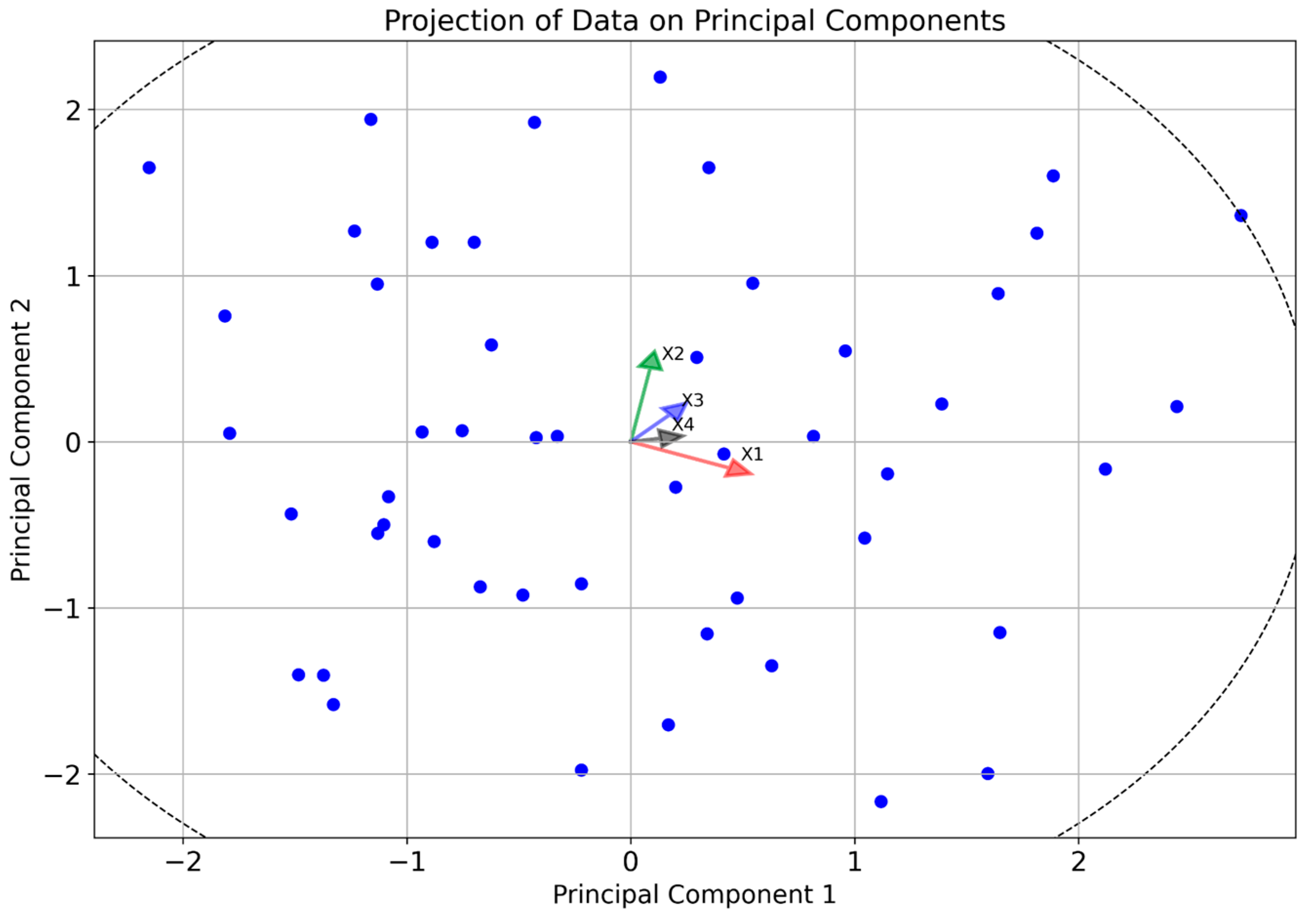
Projection onto principal components:

Finally, the standardized data matrix Z is projected onto the following new k-dimensional subspace defined by the principal components:

$$\mathit{Y}=\mathit{Z}{\mathit{V}}_{\mathit{k}}$$

(5)

where Y is the m × k matrix of the principal component scores.

The application of the statistical method PCA with is done using the MATLAB tool in this case, and the results found are included. The relation between the parameters Y_i was evaluated, as shown in Figure 13.

Figure 13. PCA of the parameters Y_i.

Principal component axes:

• The horizontal axis represents the first principal component (PC1), which explains the maximum variance in the data.
• The vertical axis represents the second principal component (PC2), which explains the second largest amount of variance, independently of PC1.

Vectors Y₁, Y₂, Y₃, and Y₄:

The colored vectors represent the original variables representing each parameter of the 3D matrix Y_i projected in the principal component space.

• The direction and length of each vector indicates how each factor is correlated with the principal components.
• For example, vector Y₁ is strongly correlated with PC1, while Y₂ has a significant component on PC2.

Blue points:

The projection of each blue point is determined by the values of PC1 and PC2 for that observation. Each point represents an observation (or individual) in the new space of components.

Correlation circle:

Vectors inside the circle indicate variables that have a strong contribution to the variance explained by the principal components. The circle represents the possible correlation.

The relative contributions of the variables (parameters Y_i) are as follows:

• Y₁: 66.5732%;
• Y₂: 32.9541%;
• Y₃: 0.47268%;
• Y₄: $3.214\times {10}^{-15}\mathrm{\%}$.

The analysis of the sub-parameters aims to identify the root cause of the factors responsible for the shown variability in Y₁ as shown in Figure 14.

Figure 14. PCA of the parameters X_1j.

The relative contributions of the variables are as follows:

• X₁₁: 99.9912%;
• X₁₂: 0.0087739%;
• X₁₃: 0%;
• X₁₄: 0%.

5.3.2. Correlation Study Application

Several statistical approaches can be employed to evaluate the relationship between the parameters X_ij, including the method of least squares. Correlation analyses are a robust and relatively straightforward way to assess interdependence links [59]. We can determine the nature of the relationship linking these parameters by calculating the correlation coefficient among the parameters X_ij. This correlation is measured using the correlation coefficient r, which is defined by the following mathematical formula:

$$\mathit{r}={\displaystyle \frac{\sum \left(\mathit{X}-\overline{\mathit{X}}\right)\times (\mathit{Y}-\overline{\mathit{Y}})}{\sqrt{{\sum (\mathit{X}-\overline{\mathit{X}})}^2\times \sum {(\mathit{Y}-\overline{\mathit{Y}})}^2}}}$$

(6)

where

• X = is a parameter that can take many values.
• $\overline{\mathit{X}}$ = is the average of the values of the parameter X.
• Y = is a second parameter that can take many values.
• $\overline{\mathit{Y}}$ = is the average of the values of a second parameter Y.

The correlation coefficient can take values between −1 and 1, i.e.,:

• r = +1 means positive correlation.
• r = 0 means absence of correlation.
• r = −1 means negative correlation.

Figure 15 provides an analysis of the link types between key parameters (Y_i, X_ij) influencing assembly line balancing. Each cell represents the correlation coefficient between two parameters of the 3D matrix.

Figure 15. Correlation study of parameters Y_i and X_ij.

Negative Correlations:

• The link type between X₁₂ and X₁₁ (−0.59) shows that as task duration (X₁₂) increases, production cadence (X₁₁) decreases.
• The inverse correlation between Y₂ and X₁₂ (−0.54) suggests that longer task durations negatively impact efficiency metrics related to the workforce or process speed.

Strong Positive Correlations:

• The parameters X₂₂ and X₃₁ expose a near-perfect correlation (~1.00), meaning that changes in shift-related factors (X₂₂) directly impact production cycle time (X₃₁).
• Similarly, X₃₁ and X₃₂ show a correlation of 1.00, reinforcing the idea that the Takt time and production cycle are intrinsically linked.

High Correlation Between Efficiency and Key Operational Metrics:

• The efficiency-related factor Y₄ is strongly correlated with X₃₁ and X₃₂ (0.96 each). This suggests that production time and demand fluctuations directly impact overall efficiency.

Low to Moderate Correlations:

• Some variables exhibit weak or negligible correlations (e.g., Y₁ and X₁₄ (0.38), or Y₁ and X₄₁ (0.10)). This indicates that factors such as material routing or secondary task dependencies have minimal direct influence on overall assembly line efficiency.
• However, their indirect effects should not be overlooked, as they may play a role in localized inefficiencies.

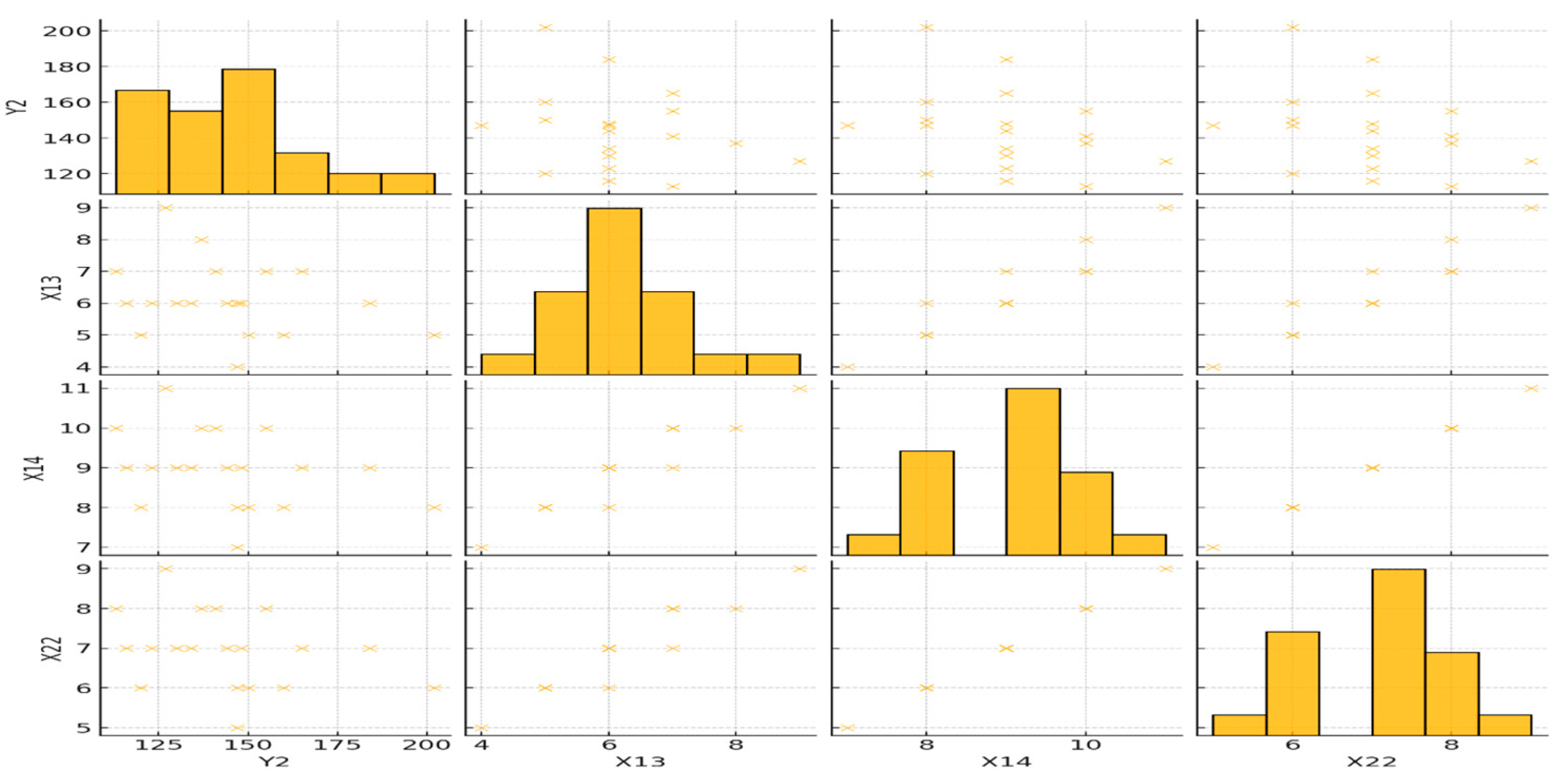
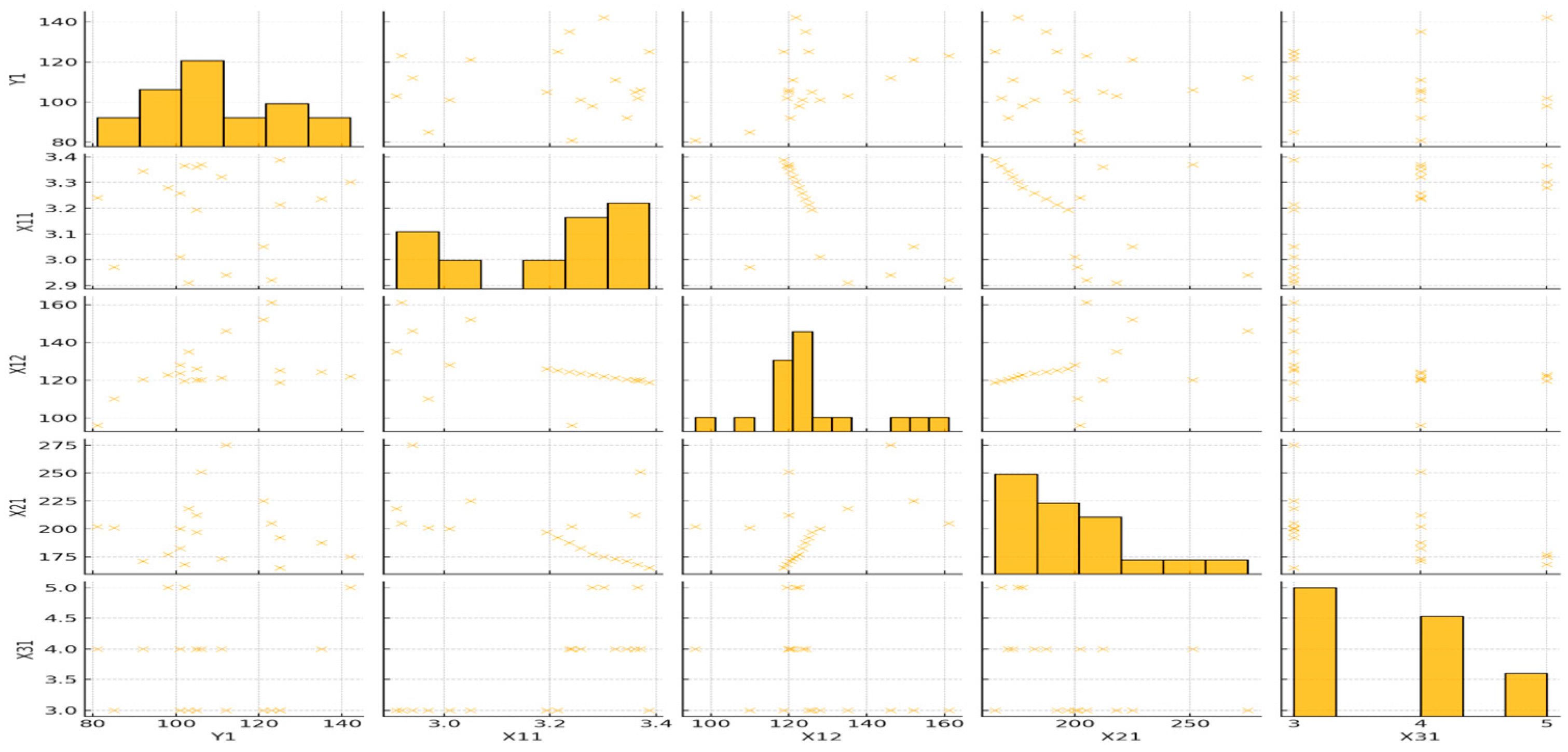
5.3.3. Graphical Representation Application

From the graph depicting, in Figure 11, the three curves of parameters Y₁, Y₂, and Y₄, it is evident that Y₁ (Efficiency) and Y₂ (Time required for constructing a beam) have a substantial impact on the overall balancing parameter Y.

Figure 16, Figure 17 and Figure 18 represent pairwise scatter plots and histograms of key process parameters in an assembly line system. The objective of such visualizations is to analyze variable distributions, dependencies, and correlations between different X_ij and Y_i parameters.

Figure 16. Pairwise correlation analysis between Y₂ and production parameters (X₁₃, X₁₄, and X₂₂).

Figure 17. Scatter matrix of Y₄ with production variables X₄₁ and X₄₂.

Figure 18. Pairwise distribution of Y₁ with task-related parameters (X₁₁, X₁₂, X₃₁, and X₃₂).

Parameter Distribution and Stability

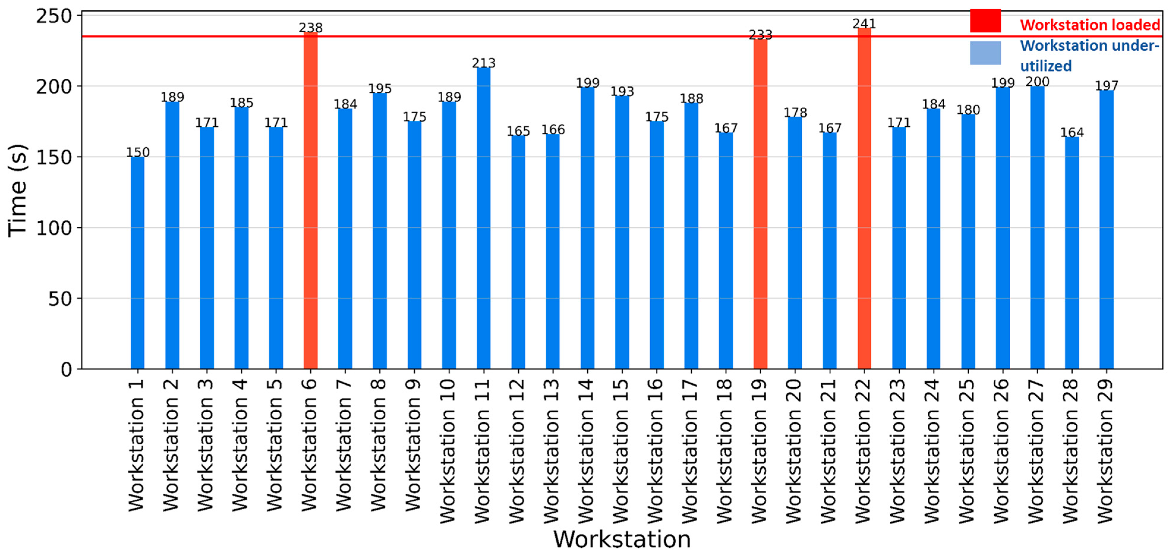
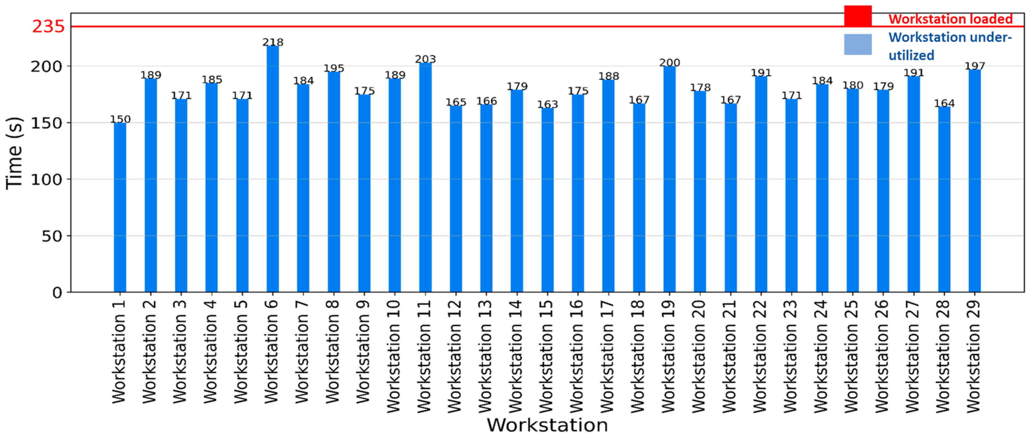
• Some parameters (X₄₂ and X₂₂) show highly structured distributions, indicating controlled operational constraints.
• Others (X₄₁ and X₁₄) exhibit wider distributions, suggesting greater variability in their impact.

Variable Influences and Dependencies

• X₃₁ and Y₂ show a strong relationship, meaning that Takt time plays a critical role in production efficiency.
• X₁₃ correlates with Y₂, suggesting that operator productivity affects manufacturing time.

Process Optimization Potential

• Workforce efficiency and Takt time adjustments should be prioritized for process improvement.
• Product-related parameters (X₄₁) should be further analyzed for potential standardization or optimization.

6. Results and Discussion

6.1. Results of Our Approach

Using the three methods of correlation, PCA, and graphical representation, we obtained the following results which can be seen in Table 3 below.

Table 3. The findings and interpretation of the application of the statistical methods.

The Statistical Method Used	Results	Interpretation
The graphical interpretation	❖ X11: Cadence: Number of conforming bundles made per time. ❖ X12: Range time: Fixed index which expresses the duration of a cycle of assembly until the final control. ❖ X21: Shift time bottleneck.	Y1 (Efficiency) variability caused by the fluctuation of X11 and X12. Y2 (The time allocated to manufacture a beam) variability caused by the parameter X21.
The correlation study	❖ X11: Cadence: Number of conforming bundles made per time. ❖ X12: Range time: Fixed index which expresses the duration of a cycle of assembly until the final control.	Y1 (Efficiency) variability caused by the fluctuation of parameter X11.
Principal component analysis study	❖ X11: Cadence: Number of conforming bundles made per time.	Y1 (Efficiency) variability caused by the fluctuation of X11 and X12.

The three employed methodologies demonstrate that the sub-parameter X₁₁ is a significant source of variability in the Y₁ parameter. However, the graphical representation method shows that the sub-parameter X₁₂ also exhibits an influence on the variability of the Y₁ parameter. Furthermore, sub-parameter X₂₁ exhibits substantial variability concerning the Y₂ parameter.

The correlation method gives matching results with the graphical representation approach, with the exception of sub-parameter X₂₁, which is excluded because of its minimal impact on variability.

In contrast, PCA indicates that sub-parameter X₁₁ demonstrates significant fluctuation, affecting the Y₁ parameter and so automatically influencing the variability of the overall parameter Y (balance efficiency). To evaluate the consequences of the results obtained from every approach, we performed a parameter changes analysis on those showing significant variability, as illustrated in the following figures.

6.1.1. Graphical Representation Interpretation

The variability graph presented in the Figure 19 blow shows that the assembly line under study exhibits five distinct workstations—namely stations 2, 6, 11, 19, and 22—that act as key bottlenecks. Analyzing parameter variability through the graphical representations “X₁₁, X₁₂, and X₂₁” demonstrates that fluctuations in these parameters markedly affect assembly line balancing. This influence leads to the formation of the identified bottlenecks and, consequently, slows down the production flow.

Figure 19. Variability study after varying X₁₁, X₁₂, and X₂₁.

6.1.2. Correlation Study Interpretation

The variability graph illustrated in the Figure 20 indicates the clear presence of two significant bottlenecks at designated workstations within the examined assembly line. These bottlenecks have been identified as workstations 6, 11, 19, and 22. The investigation into parameter variability was undertaken through the utilization of the prescribed correlation study, “X₁₁, X₁₂”.

Figure 20. Variability study after varying X₁₁ and X₁₂.

6.1.3. Principal Component Analysis Interpretation

The variability chart depicted in the Figure 21 below reveals the conspicuous existence of two prominent bottlenecks located at specific workstations within the analyzed assembly line. Workstations 19 and 22 have been identified as bottlenecks. Parameter variability was explored in a manner consistent with “X₁₁” using PCA methodology.

Figure 21. Variability study after varying X₁₁.

6.2. Discussion

Section 6.2 presents a comparative study between our multi-criteria variability analysis approach and a reference method based solely on average task execution times for balancing.

In order to quantify the added value of our approach, we set up a controlled comparison protocol between:

• Method A—reference: balancing based on mean task times alone, without taking into account dispersion or correlations between factors;
• Method B—proposed: multi-criteria variability analysis simultaneously integrating the standard deviation, coefficient of variation, and relative weight of each parameter on the overall balancing indicator Y.

Both methods were applied to an identical dataset comprising 7280 instances simulating five weeks of production, with injection of realistic disturbances (supply hazards, operator fatigue, and tool reconfiguration). For each instance, we identified the critical variables, generated a rebalancing plan, and then assessed performance over a one-week horizon of disrupted operation. Results were aggregated over 10 replications to neutralize stochastic effects; observed differences are statistically significant at the 5% level (two-tailed t-test).

Table 4 summarizes these comparative results, highlighting the performance gains achieved by the proposed method compared with the reference method.

Table 4. Comparison of Line Balancing Performance.

Indicator	Method A (Average Times)	Method B (Our Approach)
Critical variables correctly detected	2/5	5/5
Balancing efficiency after disturbance	75 ± 1.8%	84 ± 1.5%
Average number of persistent bottlenecks	3.4	1.2
Average rate of underutilization (%)	14%	7%
Average cycle time per shift (s)	54.2	48.0

These results show that Method B does the following:

• Identifies all five variables actually responsible for fluctuations, whereas the reference method reveals only two;
• Reduces disturbance-induced efficiency loss by over 12% (84% vs. 75%);
• Almost triples the number of persistent bottlenecks and halves job under-employment, reflecting better load distribution.

In practice, the integration of statistical methods within the use of the dispersion and relative importance of parameters enables corrective actions (task reallocation, rate balancing, and selective buffering) to be targeted more finely. This additional depth of process translates directly into a measurable improvement in overall line performance, confirming the relevance and robustness of our approach in the face of real industrial hazards.

7. Conclusions

In conclusion, our investigation has delved into the intricate variability of parameters crucial for assembly line balancing. The necessity for dynamic balancing is a reaction to the changing industrial environment, especially the increased demand for customized products, highlighting the importance of flexibility and agility in assembly line operations. Identifying the critical elements characterized by high variability stands as a pivotal step in achieving and maintaining dynamic balance.

Our study emphasizes the necessity of assembly lines adapting to changing control settings to address the escalating demand for customized items. An understanding of critical factors with substantial variability that directly affect assembly line balance establishes a fundamental framework for achieving dynamic balance. The mentioned elements are essential contributions to the overall balance of variety. Building on the analysis, these factors have emerged as pivotal influences on overall variability balance. They are identified through a manual process involving statistical analyses and a 3D matrix representation within MATLAB. There are, however, several limitations to this study that should be highlighted. Firstly, our analysis is highly dependent on the quality and frequency of data collection, which may affect the robustness of the results. Secondly, the influence of unobserved latent factors cannot be ruled out, which could bias some of the relationships highlighted. Finally, the feedback mechanism we have set up is not yet automated, which limits the system’s ability to react quickly to detected variations. This work naturally extends to proposing a dynamic balancing algorithm. By leveraging the framework designed to detect “root parameters” that drive variability in assembly line balancing, the next phase involves integrating multi-agent systems. This integration aims to enable real-time balancing as soon as any fluctuations are detected.

References

- Ren, W.; Wen, J.; Guan, Y.; Hu, Y. Research on Assembly Module Partition for Flexible Production in Mass Customization. Procedia CIRP 2018, 72, 744–749. [Google Scholar] [CrossRef]
- Tsutsui, S.; Kaihara, T.; Kokuryo, D.; Fujii, N.; Harano, K. A Proposal of Production Scheduling Method with Dynamic Parts Allocation for Mass Customization. Procedia CIRP 2022, 107, 882–887. [Google Scholar] [CrossRef]
- Bastos, N.M.; Alves, A.C.; Castro, F.X.; Duarte, J.; Ferreira, L.P.; Silva, F.J.G. Reconfiguration of Assembly Lines Using Lean Thinking in an Electronics Components’ Manufacturer for the Automotive Industry. Procedia Manuf. 2021, 55, 383–392. [Google Scholar] [CrossRef]
- Salveson, M.E. The Assembly-Line Balancing Problem. J. Fluids Eng. 1955, 77, 939–947. [Google Scholar] [CrossRef]
- Espinoza Pérez, A.T.; Rossit, D.A.; Tohmé, F.; Vásquez, Ó.C. Mass Customized/Personalized Manufacturing in Industry 4.0 and Blockchain: Research Challenges, Main Problems, and the Design of an Information Architecture. Inf. Fusion 2022, 79, 44–57. [Google Scholar] [CrossRef]
- Battaïa, O.; Otto, A.; Sgarbossa, F.; Pesch, E. Future Trends in Management and Operation of Assembly Systems: From Customized Assembly Systems to Cyber-Physical Systems. Omega 2018, 78, 1–4. [Google Scholar] [CrossRef]
- Li, Z.; Janardhanan, M.N.; Rahman, H.F. Enhanced Beam Search Heuristic for U-Shaped Assembly Line Balancing Problems. Eng. Optim. 2021, 53, 594–608. [Google Scholar] [CrossRef]
- Troise, C.; Corvello, V.; Ghobadian, A.; O’Regan, N. How Can SMEs Successfully Navigate VUCA Environment: The Role of Agility in the Digital Transformation Era. Technol. Forecast. Soc. Change 2022, 174, 121227. [Google Scholar] [CrossRef]
- Zhang, W.; Hou, L.; Jiao, R.J. Dynamic Takt Time Decisions for Paced Assembly Lines Balancing and Sequencing Considering Highly Mixed-Model Production: An Improved Artificial Bee Colony Optimization Approach. Comput. Ind. Eng. 2021, 161, 107616. [Google Scholar] [CrossRef]
- Gilles, M.A.; Gaudez, C.; Savin, J.; Remy, A.; Remy, O.; Wild, P. Do Age and Work Pace Affect Variability When Performing a Repetitive Light Assembly Task? Appl. Ergon. 2022, 98, 103601. [Google Scholar] [CrossRef]
- Gräßler, I.; Roesmann, D.; Cappello, C.; Steffen, E. Skill-Based Worker Assignment in a Manual Assembly Line. Procedia CIRP 2021, 100, 433–438. [Google Scholar] [CrossRef]
- Karas, A.; Ozcelik, F. Assembly Line Worker Assignment and Rebalancing Problem: A Mathematical Model and an Artificial Bee Colony Algorithm. Comput. Ind. Eng. 2021, 156, 107195. [Google Scholar] [CrossRef]
- Khan, S.H.; Majid, A.; Yasir, M. Strategic Renewal of SMEs: The Impact of Social Capital, Strategic Agility and Absorptive Capacity. Manag. Decis. 2020, 59, 1877–1894. [Google Scholar] [CrossRef]
- Andrés-López, E.; González-Requena, I.; Sanz-Lobera, A. Lean Service: Reassessment of Lean Manufacturing for Service Activities. Procedia Eng. 2015, 132, 23–30. [Google Scholar] [CrossRef]
- Nallusamy, S. Execution of Lean and Industrial Techniques for Productivity Enhancement in a Manufacturing Industry. Mater. Today Proc. 2020, 37, 568–575. [Google Scholar] [CrossRef]
- Çelik, M.T.; Arslankaya, S. Solution of the Assembly Line Balancing Problem Using the Rank Positional Weight Method and Kilbridge and Wester Heuristics Method: An Application in the Cable Industry. J. Eng. Res. 2023, 11, 100082. [Google Scholar] [CrossRef]
- Moncayo-Martínez, L.A.; Arias-Nava, E.H. Assessing by Simulation the Effect of Process Variability in the SALB-1 Problem. AppliedMath 2023, 3, 563–581. [Google Scholar] [CrossRef]
- Ragazzini, L.; Saporiti, N.; Negri, E.; Rossi, T.; Macchi, M.; Pirovano, G. A Digital Twin-Based Approach to the Real-Time Assembly Line Balancing Problem. In Proceedings of the 2nd International Conference on Innovative Intelligent Industrial Production and Logistics, Valletta, Malta, 25–27 October 2021; SCITEPRESS-Science and Technology Publications: Lisbon, Portugal, 2021; pp. 93–99. [Google Scholar]
- Hazır, Ö.; Dolgui, A. (PDF) A Review on Robust Assembly Line Balancing Approaches. IFAC-PapersOnLine 2019, 52, 987–991. [Google Scholar] [CrossRef]
- Nikkerdar, M. Smart Adaptable Assembly Line Rebalancing. Ph.D. Thesis, University of Windsor, Windsor, ON, Canada, 2025. [Google Scholar]
- Fisel, J.; Exner, Y.; Stricker, N.; Lanza, G. Changeability and Flexibility of Assembly Line Balancing as a Multi-Objective Optimization Problem. J. Manuf. Syst. 2019, 53, 150–158. [Google Scholar] [CrossRef]
- Zacharia, P.T.; Nearchou, A.C. The Fuzzy Assembly Line Worker Assignment and Balancing Problem. Cybern. Syst. 2020, 52, 221–243. [Google Scholar] [CrossRef]
- Kumar, N.; Mahto, D. Assembly Line Balancing: A Review of Developments andTrends in Approach to Industrial Application. Glob. J. Res. Eng. Ind. Eng. 2013, 13, 29–50. [Google Scholar]
- Sarwar, F. Multi-Objective Assembly Line Balancing Problem under Uncertainty Using Genetic Algorithm. Int. J. Serv. Oper. Manag. 2019, 34, 33–47. [Google Scholar] [CrossRef]
- Alavidoost, M.H.; Tarimoradi, M.; Zarandi, M.H.F. Fuzzy Adaptive Genetic Algorithm for Multi-Objective Assembly Line Balancing Problems. Appl. Soft Comput. 2015, 34, 655–677. [Google Scholar] [CrossRef]
- Zacharia, P.; Nearchou, A.C. The Robotic Assembly Line Balancing Problem under Task Time Uncertainty. Int. J. Adv. Manuf. Technol. 2025, 137, 2991–3011. [Google Scholar] [CrossRef]
- Kucukkoc, I.; Zhang, D.Z. A Mathematical Model and Genetic Algorithm-Based Approach for Parallel Two-Sided Assembly Line Balancing Problem. Prod. Plan. Control 2015, 26, 874–894. [Google Scholar] [CrossRef]
- Wu, Y. An Automated Method for Assembly Tolerance Analysis. Procedia CIRP 2020, 92, 57–62. [Google Scholar] [CrossRef]
- Boysen, N.; Schulze, P.; Scholl, A. Assembly Line Balancing: What Happened in the Last Fifteen Years? Eur. J. Oper. Res. 2022, 301, 797–814. [Google Scholar] [CrossRef]
- Hahs-Vaughn, D.L. Foundational Methods: Descriptive Statistics: Bivariate and Multivariate Data (Correlations, Associations). In International Encyclopedia of Education, 4th ed.; Elsevier: Amsterdam, The Netherlands, 2023; pp. 734–750. [Google Scholar] [CrossRef]
- Jia, G.; Zhang, Y.; Shen, S.; Liu, B.; Hu, X.; Wu, C. Load Balancing of Two-Sided Assembly Line Based on Deep Reinforcement Learning. Appl. Sci. 2023, 13, 7439. [Google Scholar] [CrossRef]
- Bottani, E.; Montanari, R.; Volpi, A.; Tebaldi, L. Statistical Process Control of Assembly Lines in Manufacturing. J. Ind. Inf. Integr. 2023, 32, 100435. [Google Scholar] [CrossRef]
- Chen, H.; Li, X.; Jin, S. A Statistical Method of Distinguishing and Quantifying Tolerances in Assemblies. Comput. Ind. Eng. 2021, 156, 107259. [Google Scholar] [CrossRef]
- Tian, A.; Shu, X.; Guo, J.; Li, H.; Ye, R.; Ren, P. Statistical Modeling and Dependence Analysis for Tide Level via Multivariate Extreme Value Distribution Method. Ocean Eng. 2023, 286, 115616. [Google Scholar] [CrossRef]
- Bortolini, M.; Ferrari, E.; Gamberi, M.; Pilati, F.; Faccio, M. Assembly System Design in the Industry 4.0 Era: A General Framework. IFAC-PapersOnLine 2017, 50, 5700–5705. [Google Scholar] [CrossRef]
- Li, X.; Athinarayanan, R.; Wang, B.; Yuan, W.; Zhou, Q.; Jun, M.; Bravo, J.; Gao, R.X.; Wang, L.; Koren, Y. Smart Reconfigurable Manufacturing: Literature Analysis. Procedia CIRP 2024, 121, 43–48. [Google Scholar] [CrossRef]
- Keshvarparast, A.; Katiraee, N.; Pirayesh, A.; Battaia, O.; Berti, N. Integrated Resource Optimization in a Multi-Product Separated Line Collaborative Assembly Line Balancing Problem (MPSLC-ALBP). IFAC-PapersOnLine 2023, 56, 713–718. [Google Scholar] [CrossRef]
- Jaskó, S.; Skrop, A.; Holczinger, T.; Chován, T.; Abonyi, J. Development of Manufacturing Execution Systems in Accordance with Industry 4.0 Requirements: A Review of Standard- and Ontology-Based Methodologies and Tools. Comput. Ind. 2020, 123, 103300. [Google Scholar] [CrossRef]
- Pilati, F.; Lelli, G.; Faccio, M.; Gamberi, M.; Regattieri, A. Assembly Line Balancing for Personalized Production. IFAC-PapersOnLine 2020, 53, 10261–10266. [Google Scholar] [CrossRef]
- Hillali, Y.; Chafik, S.; Alfathi, N.; Zegrari, M. Variability and Correlation of Parameters for Dynamic Balancing of an Assembly Line Based on a Statistic Method. In Proceedings of the 2023 14th International Conference on Intelligent Systems: Theories and Applications (SITA), Mohammedia, Morocco, 22–23 November 2023; pp. 1–6. [Google Scholar]
- Hillali, Y.; Zegrari, M.; Alfathi, N.; Chafik, S.; Tabaa, M. Statistical Method Using Principal Component Analysis to Determine High Variability Parameters Affecting the Balancing of an Assembly Line. Math. Model. Comput. 2024, 11, 663–673. [Google Scholar] [CrossRef]
- Li, M.-L. An Algorithm for Arranging Operators to Balance Assembly Lines and Reduce Operator Training Time. Appl. Sci. 2021, 11, 8544. [Google Scholar] [CrossRef]
- GN, M.B. Application of Lean Line Concepts to Improve Efficiency of PE Pump Assembly Lines. Int. J. Eng. Res. 2014, 3, 1–7. [Google Scholar]
- Cuik Chapter 6 Assembly Systems And Line Balancing. Available online: https://rekadayaupaya.wordpress.com/category/computer-integrated-manufacturing/part-ii/chapter-6-assembly-systems-and-line-balancing/ (accessed on 1 July 2025).
- Hillali, Y.; Zegrari, M.; Alfathi, N.; Chafik, S. Balancing Assembly Line Based on Lean Management Tools. In Proceedings of the Smart Applications and Data Analysis, Tangier, Morocco, 18–20 April 2024; Hamlich, M., Dornaika, F., Ordonez, C., Bellatreche, L., Moutachaouik, H., Eds.; Springer Nature: Cham, Switzerland, 2024; pp. 131–144. [Google Scholar]
- Buyukozkan, K.; Kucukkoc, I.; Satoglu, S.I.; Zhang, D.Z. Lexicographic Bottleneck Mixed-Model Assembly Line Balancing Problem: Artificial Bee Colony and Tabu Search Approaches with Optimised Parameters. Expert Syst. Appl. 2016, 50, 151–166. [Google Scholar] [CrossRef]
- Zamzam, N.; El-Kharbotly, A.K. Balancing Two-Sided Multi-Manned Assembly Line under Time and Space Constraint. Ain Shams Eng. J. 2023, 15, 102464. [Google Scholar] [CrossRef]
- Fortuny-Santos, J.; Ruiz-de-Arbulo-López, P.; Cuatrecasas-Arbós, L.; Fortuny-Profitós, J. Balancing Workload and Workforce Capacity in Lean Management: Application to Multi-Model Assembly Lines. Appl. Sci. 2020, 10, 8829. [Google Scholar] [CrossRef]
- Özcan, U.; Aydoğan, E.K.; Himmetoğlu, S.; Delice, Y. Parallel Assembly Lines Worker Assignment and Balancing Problem: A Mathematical Model and an Artificial Bee Colony Algorithm. Appl. Soft Comput. 2022, 130, 109727. [Google Scholar] [CrossRef]
- Zhang, Y.; Cheng, Y.; Wang, X.V.; Zhong, R.Y.; Zhang, Y.; Tao, F. Data-Driven Smart Production Line and Its Common Factors. Int. J. Adv. Manuf. Technol. 2019, 103, 1211–1223. [Google Scholar] [CrossRef]
- Huo, J.; Chan, F.T.S.; Lee, C.K.M.; Strandhagen, J.O.; Niu, B. Smart Control of the Assembly Process with a Fuzzy Control System in the Context of Industry 4.0. Adv. Eng. Inform. 2020, 43, 101031. [Google Scholar] [CrossRef]
- Furugi, A. Sequence-Dependent Time- and Cost-Oriented Assembly Line Balancing Problems: A Combinatorial Benders’ Decomposition Approach. Eng. Optim. 2022, 54, 170–184. [Google Scholar] [CrossRef]
- Kuo, Y.; Chen, S.-H.; Yang, T.; Hsu, W.-C. Optimizing a U-Shaped Conveyor Assembly Line Balancing Problem Considering Walking Times between Assembly Tasks. Appl. Sci. 2023, 13, 3702. [Google Scholar] [CrossRef]
- Álvarez-Miranda, E.; Pereira, J.; Vilà, M. Analysis of the Simple Assembly Line Balancing Problem Complexity. Comput. Oper. Res. 2023, 159, 106323. [Google Scholar] [CrossRef]
- Wang, J.; Swartz, C.L.E.; Corbett, B.; Huang, K. Supply Chain Monitoring Using Principal Component Analysis. Ind. Eng. Chem. Res. 2020, 59, 12487–12503. [Google Scholar] [CrossRef]
- Schlüter, M.J.; Ostermeier, F.F. Dynamic Line Balancing in Unpaced Mixed-Model Assembly Lines: A Problem Classification. CIRP J. Manuf. Sci. Technol. 2022, 37, 134–142. [Google Scholar] [CrossRef]
- Qiang, Y.; Xie, S.; Li, L.; Xia, H.; Chen, Y. Application of Dimension Reduction Methods on Propeller Performance Prediction Model. Ocean Eng. 2024, 291, 116310. [Google Scholar] [CrossRef]
- Yan, R.; Gao, R.X.; Chen, X. Wavelets for Fault Diagnosis of Rotary Machines: A Review with Applications. Signal Process. 2014, 96, 1–15. [Google Scholar] [CrossRef]
- Lai, X.; Qiu, T.; Shui, H.; Ding, D.; Ni, J. Predicting Future Production System Bottlenecks with a Graph Neural Network Approach. J. Manuf. Syst. 2023, 67, 201–212. [Google Scholar] [CrossRef]