1. Introduction
In control theory, several foundational problems such as stabilization [
1,
2], controllability [
3,
4], and optimal control have been extensively studied due to their relevance across a wide range of applications. In many practical scenarios, particularly electrical systems [
5,
6], aerospace engineering [
7,
8], and process automation [
9,
10], disturbances act as unavoidable sources of deviation from nominal system behavior. These disturbances may arise from modeling inaccuracies, environmental influences, or imperfections in sensors and actuators [
11]. Although full-state stabilization offers a degree of robustness, it often proves inadequate when the focus is on output performance.
The challenge of disturbance rejection has garnered significant scholarly attention, establishing itself as a pivotal area within modern control theory, with robust contributions spanning both theoretical frameworks and practical applications. Prior investigations have explored various facets of this problem. For instance, Bouyaghroumni et al. [
12] meticulously examined admissible disturbance sets pertinent to perturbed discrete-time systems, while Rachik et al. [
13] provided an insightful analysis of nonlinear admissible disturbances within discrete nonlinear systems. Concurrently, Bourlès et al. [
14] addressed the imperative of robust stabilization in discrete-time periodic linear systems, with a particular emphasis on integrated tracking and disturbance rejection strategies.
In more recent advancements, particularly within the domain of sophisticated control techniques, several researchers have leveraged advanced methodologies for disturbance handling. Jijun et al. [
15] demonstrated the efficacy of improved genetic algorithms integrated into active disturbance rejection control (ADRC) frameworks for enhanced quadcopter stabilization. Complementing this, Han et al. [
16] presented a detailed study on an improved active disturbance rejection control methodology specifically tailored for two-degree-of-freedom serial flexible manipulators. Furthermore, Luo et al. [
17] innovated by developing a deep reinforcement learning-based active disturbance rejection control scheme for the precise position and attitude control of remotely operated vehicles (ROVs). Michalski et al. [
18] contributed by introducing an adaptive active disturbance rejection control approach incorporating recursive parameter identification. Lastly, Shen et al. have made notable contributions to the field of NPC converters, proposing both fixed-time sliding mode control [
19] and finite-time sliding mode control [
20] strategies that significantly improve disturbance rejection and compensation performance, respectively.
In this context, and in order to contribute further to the ongoing discourse on robust control design, we investigate the problem of disturbances acting on the initial conditions of continuously controlled linear systems. More precisely, we consider the following system dynamics:
where
is the state matrix,
is the control input matrix, and the initial state
is composed of a known nominal component
and an unknown perturbation
. The disturbance set
is typically assumed to be a bounded convex polytope, reflecting the structured uncertainty in the initial condition [
21].
From a practical perspective, it is desirable to ensure that these initial perturbations have no influence or only a marginal influence on the output of the system. Consequently, the first objective of this paper is to establish conditions under which the effect of initial disturbances is entirely canceled at the output level. In this case, the output trajectory under uncertainty coincides exactly with that of the nominal system (i.e., with ). We refer to this situation as exact rejection of disturbances. Under appropriate assumptions, we provide a complete characterization of this property and propose an algorithm capable of achieving it.
When exact rejection is not achievable, we address a more relaxed objective: to ensure that the deviation between disturbed and undisturbed outputs remains below a prescribed tolerance. We term this property the weak rejection of disturbances. In the second part of the article, we establish sufficient conditions for weak rejection to be feasible and demonstrate that, under a suitable discretization of the output signal, the problem can be effectively addressed.
The remainder of this paper is structured as follows:
Section 2 establishes the necessary and sufficient conditions for exact disturbance rejection in the continuous-time output case.
Section 3 addresses the weak rejection problem within the context of the discrete-time output scenario. Finally, a comprehensive conclusion summarizes the key findings and contributions of this work.
2. Exact Rejection of Perturbations
In this section, we focus on the problem of exact rejection of perturbations in linear systems (
1).
We aim to design feedback control laws that ensure the exact rejection of perturbations, meaning that the output trajectory of the system remains invariant despite the presence of disturbances. In this section, we assume that is a convex polytope and introduce a structural hypothesis on the perturbation set to address the problem for a specific class of configurations. Specifically, we assume that is a convex polytope with s vertices, where exactly r of its vertices are linearly independent (), and the remaining vertices can be expressed as linear combinations of these independent vertices. This implies that is contained within a hyperplane in the state space, meaning that the perturbations evolve in a subspace of dimension strictly lower than n. This hypothesis is motivated by practical considerations in robust control and uncertainty modeling, where perturbations are often subject to structural, physical constraints, or correlations that reduce their effective degrees of freedom. In real dynamic systems, perturbations cannot vary freely in the entire state space due to limitations imposed by physical capacities, system structure, or correlated uncertainties. These restrictions confine perturbations to an affine subspace of lower dimension, justifying the structural assumptions on and simplifying the analysis without compromising the representativeness of the model.
The corresponding controlled output
where
is the output matrix linking the state vector
of dimension
n to the output
of dimension
k. The matrix
models the direct influence of the input
on
.
The feedback control signals and are defined as and , where and are the respective gain matrices.
The primary objective of this study is to devise feedback control strategies
u and
v such that the system’s output
remains identical to its unperturbed counterpart
, for all perturbations
and across all time
. This goal entails finding suitable feedback matrices
K and
H in
such that
is satisfied under the influence of
within the convex polytope
. Mathematically, this is equivalent to showing that
This condition is challenging to verify or implement due to the continuous nature of time
t and the complexity of the set
. To simplify the problem, we propose a condition that eliminates the continuous time
t and only utilizes the vertices of
.
In order to render the exact disturbance rejection problem more amenable to analysis and computation, we propose the following proposition. This result, rooted in principles of linear algebra, specifically the Cayley–Hamilton theorem and the f Krein-Milman’s theorem [
21,
22,
23] reformulates the infinite-time condition into a finite set of constraints.
Proposition 1. The condition stated in (2) is equivalent to the following: Proof. Suppose condition (
3) holds. Let
denote the closed-loop system matrix. We aim to establish that
for all
and all
. By the Cayley–Hamilton theorem [
21,
22,
23], the matrix
satisfies its characteristic polynomial. Consequently, there exist coefficients
such that
By mathematical induction, every power
with
can be uniquely represented as a linear combination of the basis
in the vector space of
matrices. This fundamental property allows us to decompose the matrix exponential as
where the coefficient functions
are entire analytic functions of
t. Given the hypothesis
for all
and all vertices
, we obtain
for each vertex
. By the Krein–Milman theorem [
21,
22,
23], every element
admits a unique representation as a convex combination of the extreme points (vertices) of
, i.e.,
Exploiting the linearity of both the matrix exponential and the output operator
, we deduce
thereby establishing condition (
2).
For the converse, suppose that condition (
2) holds. Since
, the condition
holds for all
and all vertices
. Consider the function
, which is identically zero for all
. Since
is an entire analytic function of
t, the function
possesses derivatives of all orders. The vanishing of
and all its derivatives at
yields
This establishes
for all
and all vertices
, which constitutes precisely condition (
3).
The bidirectional proof establishes the claimed equivalence between the infinite-dimensional condition (
2) and the finite-dimensional condition (
3), thereby completing the demonstration. □
Remark 1. The above proposition eliminates the issue of continuous-time dependency and the complication of an infinite number of possible perturbations. Instead, the analysis is restricted to the finite set of vertices of the convex polytope Ω, thereby reducing condition (2) to a system of equations. We construct a matrix
such that
while ensuring that
M is non-zero. The construction of this matrix follows the algorithm below:
- 1.
Construct the matrix W: First, we form the matrix , where W has rank r since the vectors are linearly independent.
- 2.
Complete the basis of : We complete the set into a full basis of using an orthogonalization method such as the Gram–Schmidt process. This gives the matrix , where Q is a matrix of rank n.
- 3.
Construct the matrix
M: To obtain a matrix with the desired kernel, we define
This matrix M is non-zero and satisfies , as it maps the convex hull of the vectors to zero.
Thus, by constructing M in this manner, we ensure that the kernel of M exactly corresponds to the convex hull of the perturbation vectors while keeping the matrix M non-zero.
We construct also a non-zero matrix N such that is included in the vector space spanned by the set of vectors , for all , the following steps are followed:
- 1.
Construct the Matrix W: First, we form the matrix , where the vectors are linearly independent. This ensures that W has rank r.
- 2.
Define the Projection Transformation: To ensure that lies within the vector space spanned by , we define a transformation T that projects each onto this subspace. This projection can be achieved by a matrix P, which effectively reduces the dimensions of the vectors to the subspace spanned by .
- 3.
Construct the Matrix
N: The matrix
N is then defined as
, where is a matrix that adjusts the coordinates of the vectors in the subspace spanned by these vectors. This matrix N ensures that each lies within the vector space spanned by .
By following these steps, we ensure that the matrix N satisfies the desired condition that is included in the vector space spanned by for every .
The following lemma, employed in [
24], the proofs provided in references [
25,
26].
Lemma 1. Consider the matrix equationwhere , are given matrices, and is the unknown matrix. The matrix equation has a solution X if and only if Proposition 2. Let M and N be the matrices defined respectively in (6) and (7). If the following rank conditions are satisfiedthen there exist matrices H and K such that the state-feedback controls and ensure that the condition (2) is satisfied. Proof. We aim to determine two matrices
H and
K such that the objective (
3) is satisfied.
Let
M be the matrix constructed as in (
6) using our algorithm. Consider the following matrix equation
That is,
Using the fact that
and by Lemma 1, there exists a matrix
satisfying this equation.
By the construction of
M, we have:
Indeed, the vectors
belong to
, and the vectors
are linear combinations of
. Thus, the objective (
3) is verified for
.
Now consider the matrix
N constructed by Equation (
7), which satisfies the condition that for each
, the image of
under
N lies in the vector space spanned by
. Using Lemma 1 again and the fact that
there exists a matrix
such that
It follows that for all
,
Consequently, for every
and for all
, we have
In particular, by considering the state feedback controls defined by
and
, the associated feedback laws ensure the exact rejection of the disturbance of (
1). □
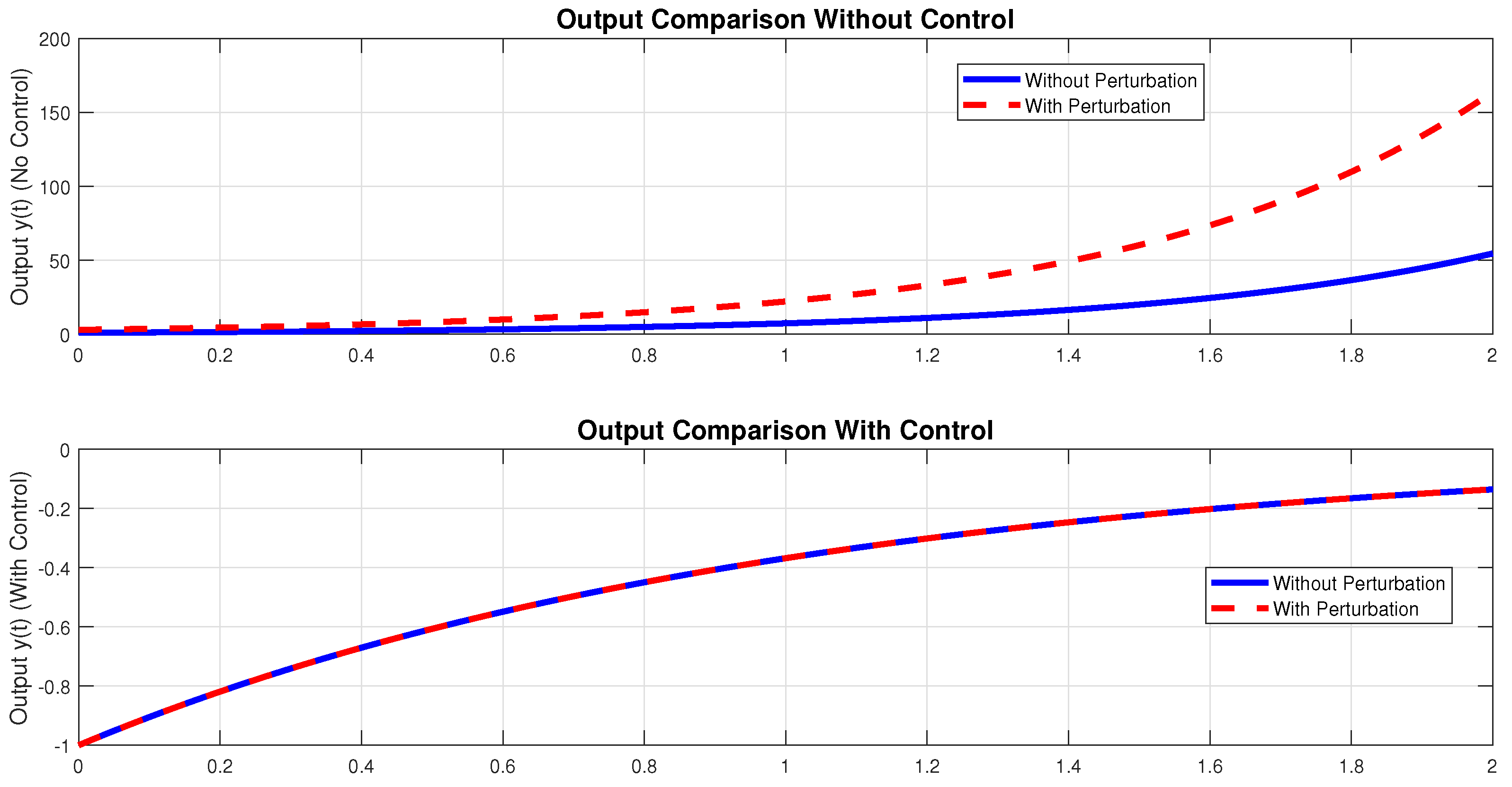
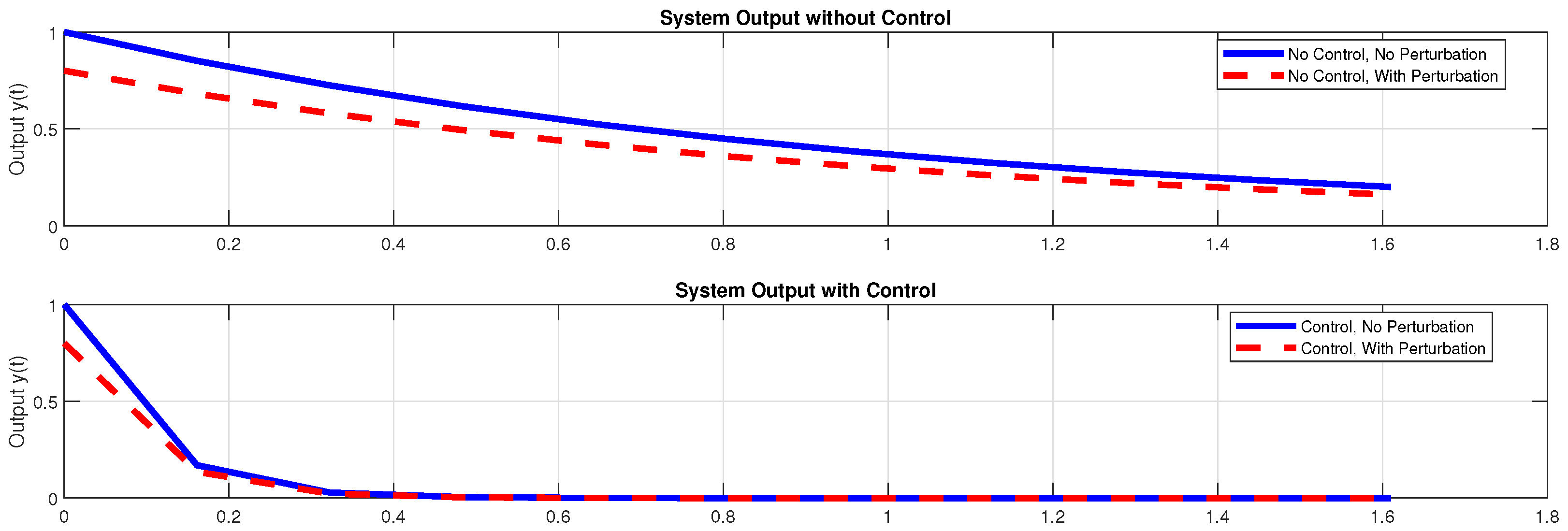
Remark 2. Under the conditions of Proposition (2), even though the number of linearly independent vertices of the polytope is equal to the dimension of the state space n, our algorithm ensures exact disturbance rejection. However, these same conditions also lead to the cancellation of the outputs; that is, for all i and for all ω. Example 1. We consider the case where and define the following matricesLet and with . We take , which satisfies . Moreover, we computeTherefore, there exists a matrix such that . For instance, the matrixsatisfies this condition. On the other hand, consider the matrixWe verify that , and compute:Hence, there exists a matrix such that . For example, the matrixsatisfies the condition. Consequently, by choosing the feedback controls and , the condition (2) is satisfied. Figure 1 clearly illustrates the effectiveness of the proposed feedback control strategy using the inputs
u and
v. In the top subplot, where no control is applied, we observe a significant divergence between the perturbed output (red dashed line) and the unperturbed output (solid blue line), indicating the substantial impact of external disturbances on the system’s behavior. In contrast, the bottom subplot shows the output evolution under the action of the designed feedback controls. Here, the perturbed and unperturbed outputs perfectly coincide throughout the time horizon, demonstrating that the disturbance has been exactly rejected by the control strategy. This confirms that our method achieves an
exact output disturbance rejection, ensuring robust output performance despite the presence of perturbations.
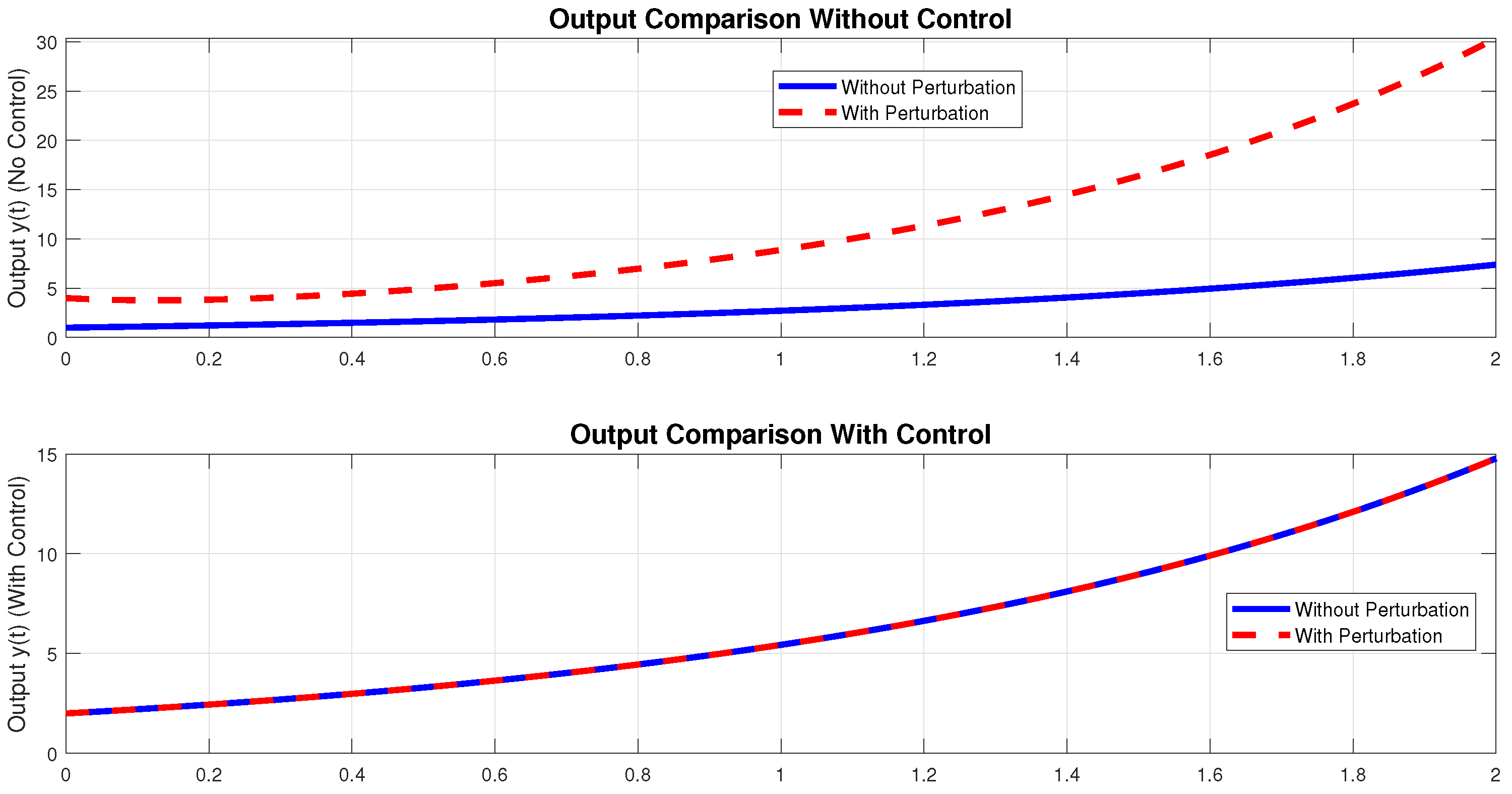
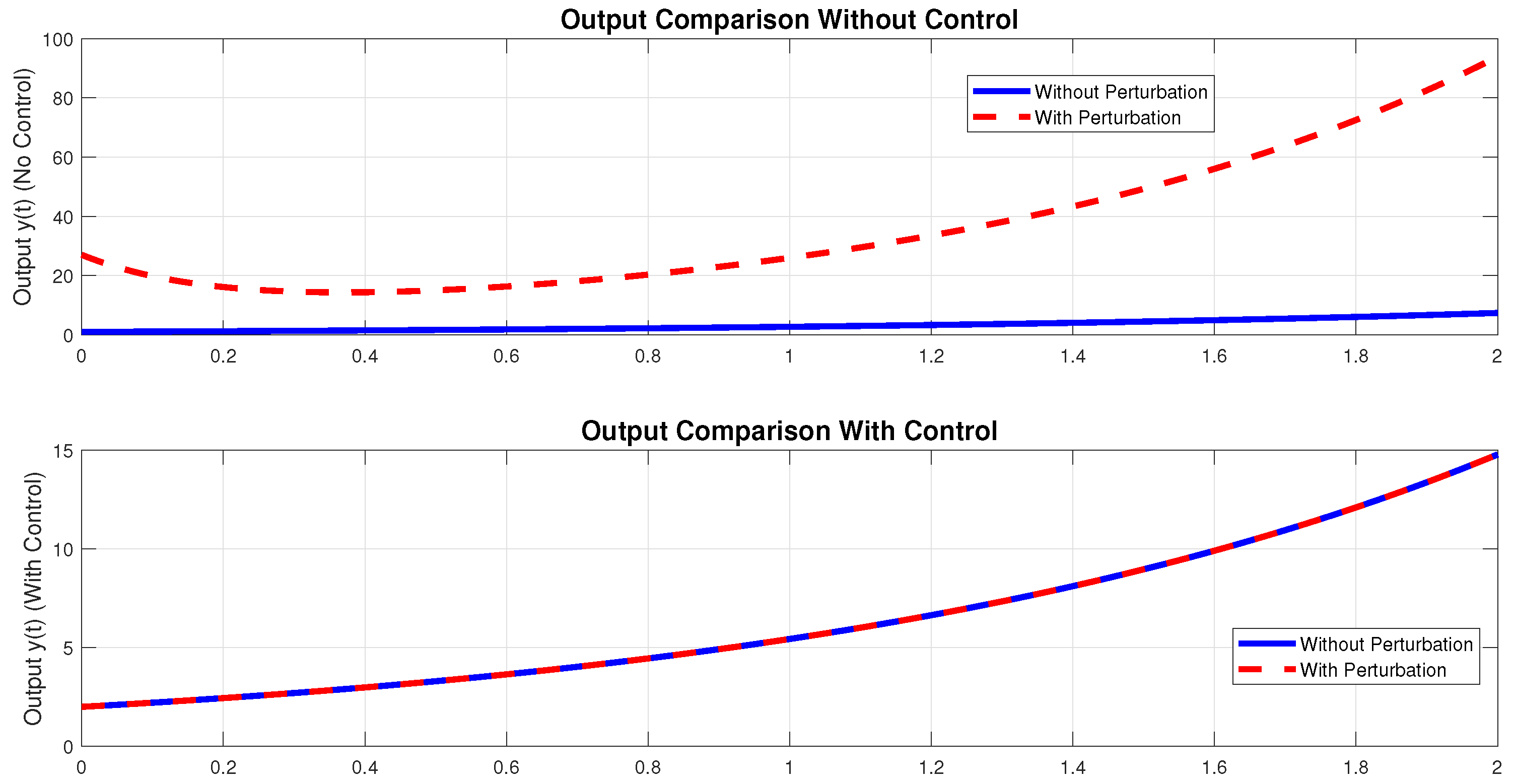
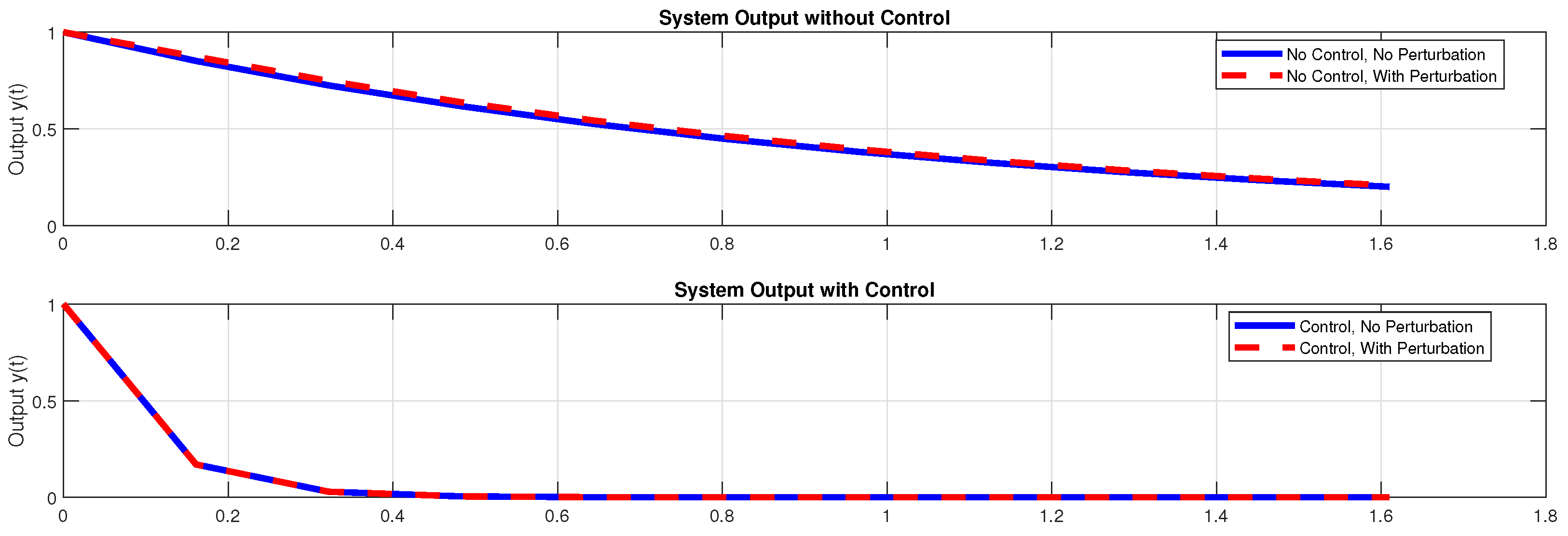
Example 2. Consider the continuous-time linear control system with the following dataWe define the perturbation vectors asfor some real scalars . Let us define the matrixThis matrix satisfies the condition , and moreover:Therefore, there exists a matrix such that . One possible solution is On the other hand, consider the matrixIt satisfies and , and we also verify that:Thus, there exists a matrix such that . One such matrix is:Consequently, by applying the state feedback control lawsthe compatibility condition (2) is satisfied. In Example (2), we considered a state-space model of dimension 3. The set of possible disturbances Ω is assumed to be generated by a finite number s of vertices, among which two, denoted and , are linearly independent. The remaining elements of Ω are linear combinations of these two vectors. Using Figure 2, Figure 3, Figure 4 and Figure 5, we demonstrated the effectiveness of our control strategy in rejecting the influence of the disturbances , , and all their linear combinations at the system output. This confirms that our method ensures robust performance with respect to the entire set Ω, thereby achieving exact rejection of the disturbances. 3. Weak Rejection of Perturbations
In this section, we consider the continuous-time linear system as described in Equation (
1). The perturbation set
is assumed to be a convex polytope with vertices
. The corresponding output is discrete and given by
where the time intervals are partitioned as
, with
.
Here,
is the output matrix, and
represents the feedback control, which is defined as
where
is the feedback gain matrix.
We address the issue of weak rejection of perturbations in a discrete-time controlled system. The objective is to design a control law such that, for any perturbation
and for a given threshold
, the following condition is satisfied:
where
.
This condition ensures that the output of the system remains close to the output in the absence of disturbances, even in the presence of perturbations , with the deviation being bounded by the threshold .
H1: Stabilizability of the Pair
Assume that the pair is stabilizable.
Now, let be a set of n distinct strictly negative real values, i.e., for all . Then, there exists a feedback gain matrix K such that the eigenvalues of are exactly given by . Furthermore, let denote the eigenvectors associated with these eigenvalues, which form a normal basis of .
Consider
as the convex hull generated by the vectors
and their opposites. Formally,
where
and
for
.
Proposition 3. If hypothesis H1 holds, and additionally,then condition (8) is satisfied. Proof. We first show that .
Let
. By definition, any
can be written as a linear combination of the eigenvectors
, i.e.,
where
for all
.
Decompose each coefficient
into its positive and negative parts:
where
and
. Substituting this decomposition, we get:
To express
in terms of the generators
of the convex cone
, let:
Thus, we can rewrite
as:
Next, define:
By construction,
. Multiply
by
:
Let
, we have
Clearly,
for all
, and we have
Thus,
is a convex combination of the generators
. Since
is a convex cone, it follows that:
Finally, because
is a cone, it is closed under positive scalar multiplication. Hence:
As
is the convex hull of
, and
is a convex set, we conclude that:
Secondly, let
for
. For
, we have:
Now, let
, and choose
sufficiently small such that:
Using the fact that
, we obtain:
Therefore, if we add the second requirement, the relationship (
8) is verified.
□
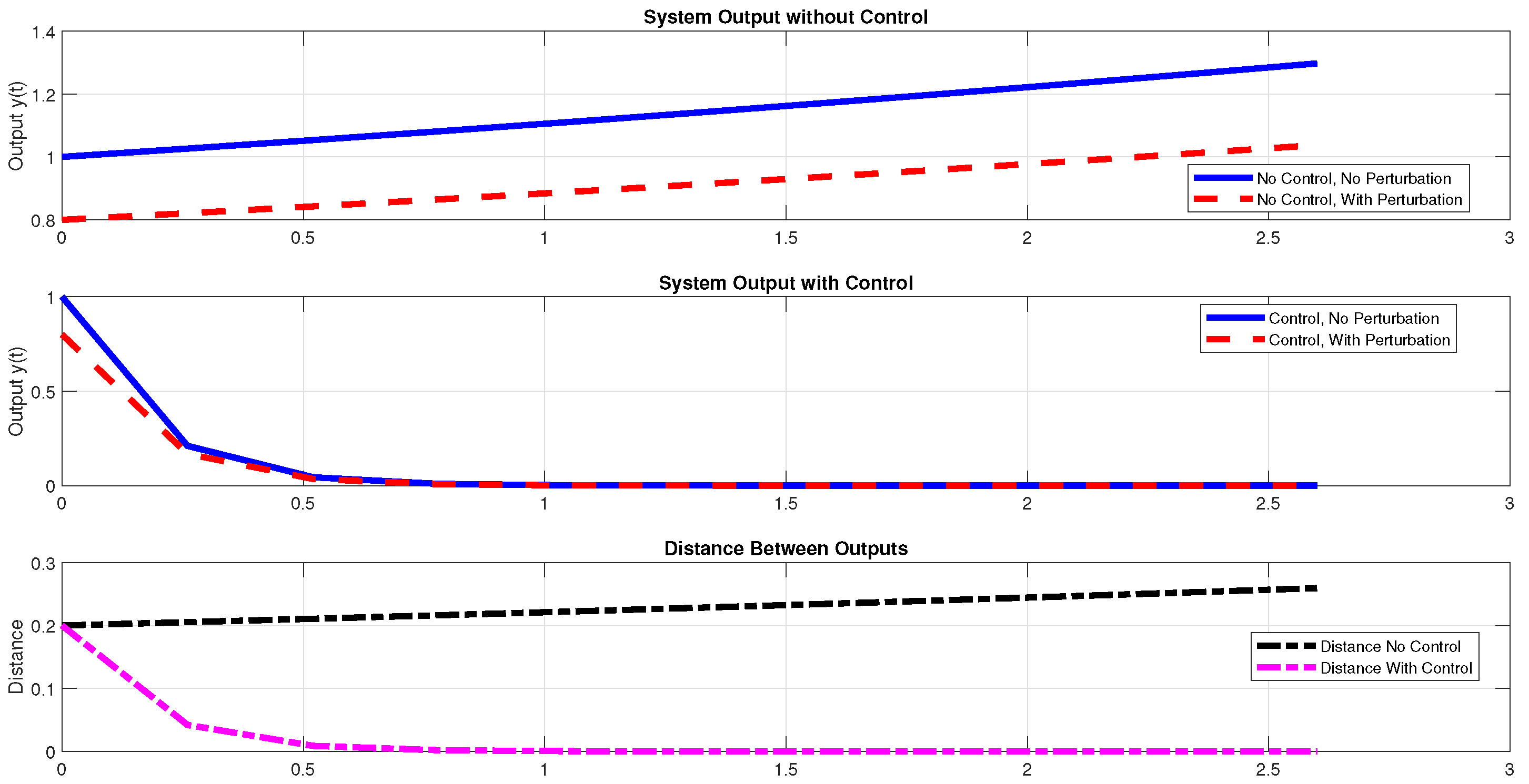
Example 3. Consider the following state-space representationwhere: Considering a polytope Ω defined by the vertices , , and , an analysis was conducted on a dynamical system initialized at , with a specified threshold . Under the consideration of a parameter and the application of a state feedback control law , where the control gain matrix is , the following simulations were obtained via MATLAB (R2020a, The MathWorks, Inc., Natick, MA, USA).
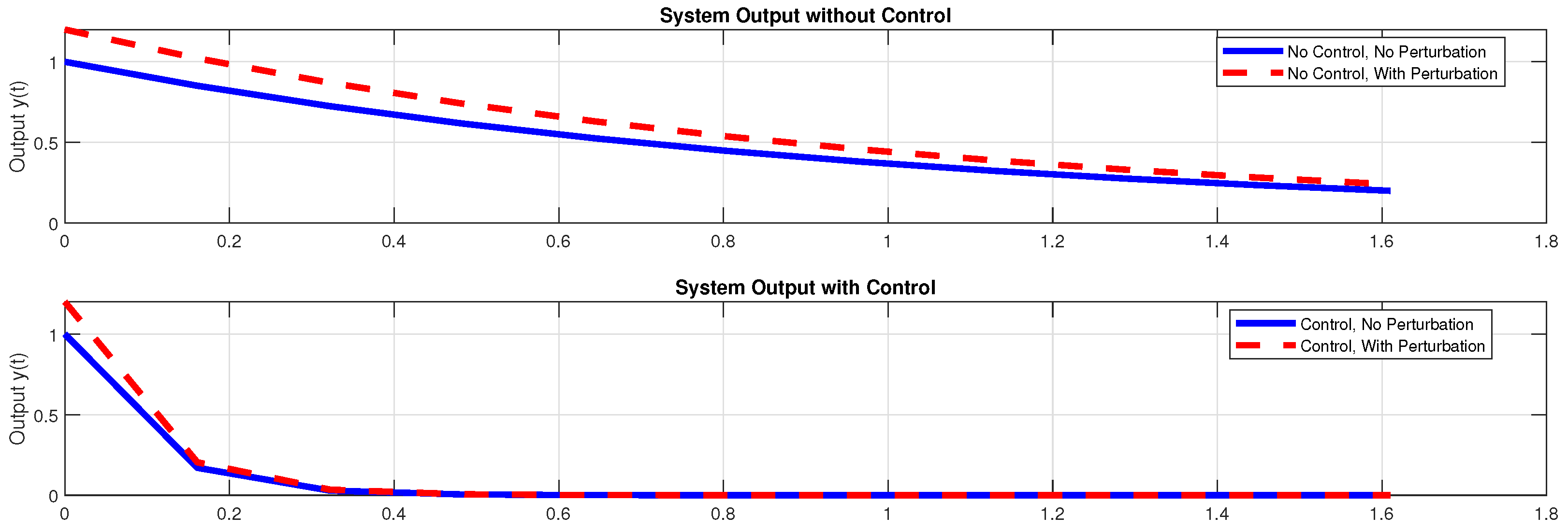
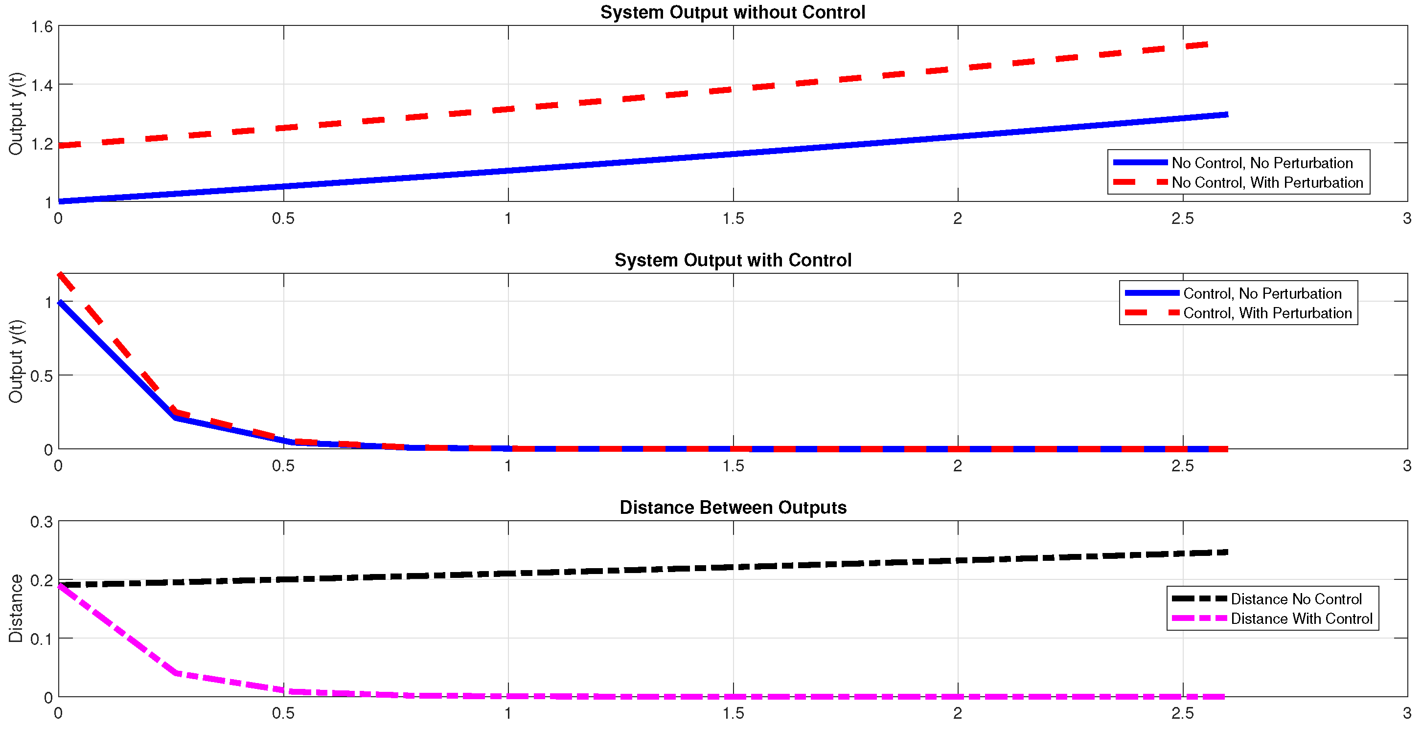
Figure 6, Figure 7 and Figure 8 present simulation results designed to verify the effectiveness of the proposed control method for weak disturbance rejection in discrete-time output systems. The comparative analysis of the system outputs with and without control reveals a clear distinction in the attenuation of disturbances. More precisely, while the uncontrolled system demonstrates a notable deviation in the output trajectories under perturbed conditions, the application of the control law considerably reduces this deviation. Moreover, the inclusion of the “Distance Between Outputs" graphs in certain figures offers a quantitative measure of the control’s performance, explicitly illustrating the convergence of the perturbed output towards the nominal trajectory. These simulation results corroborate the theoretical claim that the proposed control strategy can achieve weak disturbance rejection by maintaining the output within a predefined tolerance limit despite the presence of disturbances. Example 4. Consider the following state-space representation:where: To illustrate the efficacy of the proposed control strategy, a specific case study involving a polytope Ω, defined by the vertices , , and , was examined. For a dynamical system commencing from the initial state and subject to a threshold , a state feedback control law with a gain matrix was implemented, considering a parameter . Notably, the open-loop system exhibits instability. The subsequent simulations were generated using MATLAB to analyze the closed-loop system behavior.
The simulation results shown in Figure 9, Figure 10 and Figure 11 further emphasize the effectiveness of the proposed control strategy, particularly in scenarios involving unstable open-loop systems. In the absence of control, the inherent instability of the system leads to a significant divergence of the output trajectories when subjected to perturbations. However, the implementation of the designed control law effectively stabilizes the system and ensures that the output remains bounded within an acceptable range of the nominal output, even in the presence of perturbations. These results highlight the robustness of the control design and its ability to achieve weak disturbance rejection, even when the uncontrolled system exhibits undesirable dynamic behavior. 4. Conclusions
This study has presented a comprehensive analysis of disturbance rejection in localized continuous linear systems, addressing both exact and weak rejection paradigms. For continuous-time output systems, the paper established sufficient conditions for achieving exact perturbation rejection, demonstrating the feasibility of designing control laws that ensure output invariance despite disturbances under specific structural assumptions on the perturbation set. Furthermore, the investigation into discrete-time output systems elucidated the conditions for weak disturbance rejection, illustrating that with stabilizability and appropriate discretization, control strategies can be formulated to maintain the output within a desired tolerance. The efficacy of the proposed theoretical frameworks was corroborated through illustrative simulations, providing empirical evidence of the potential for the developed control methodologies to mitigate the impact of disturbances in linear systems. These findings contribute to the advancement of control theory by offering systematic approaches to disturbance rejection, with significant implications for practical applications in various engineering domains.
As a natural perspective, future work will aim to extend the current framework to more general settings, including the case where the perturbation is time-varying or when the state is influenced by additional external disturbances. Moreover, particular attention will be devoted to the analysis and control design for bilinear systems, which represent a natural yet more complex generalization of the linear setting. These directions open new avenues for the development of robust control strategies that remain effective under broader classes of dynamical uncertainties.
