Deep Dyna-Q for Rapid Learning and Improved Formation Achievement in Cooperative Transportation

Abstract

Nowadays, academic research, disaster mitigation, industry, and transportation apply the cooperative multi-agent concept. A cooperative multi-agent system is a multi-agent system that works together to solve problems or maximise utility. The essential marks of formation control are how the multiple agents can reach the desired point while maintaining their position in the formation based on the dynamic conditions and environment. A cooperative multi-agent system closely relates to the formation change issue. It is necessary to change the arrangement of multiple agents according to the environmental conditions, such as when avoiding obstacles, applying different sizes and shapes of tracks, and moving different sizes and shapes of transport objects. Reinforcement learning is a good method to apply in a formation change environment. On the other hand, the complex formation control process requires a long learning time. This paper proposed using the Deep Dyna-Q algorithm to speed up the learning process while improving the formation achievement rate by tuning the parameters of the Deep Dyna-Q algorithm. Even though the Deep Dyna-Q algorithm has been used in many applications, it has not been applied in an actual experiment. The contribution of this paper is the application of the Deep Dyna-Q algorithm in formation control in both simulations and actual experiments. This study successfully implements the proposed method and investigates formation control in simulations and actual experiments. In the actual experiments, the Nexus robot with a robot operating system (ROS) was used. To confirm the communication between the PC and robots, camera processing, and motor controller, the velocities from the simulation were directly given to the robots. The simulations could give the same goal points as the actual experiments, so the simulation results approach the actual experimental results. The discount rate and learning rate values affected the formation change achievement rate, collision number among agents, and collisions between agents and transport objects. For learning rate comparison, DDQ (0.01) consistently outperformed DQN. DQN obtained the maximum −170 reward in about 130,000 episodes, while DDQ (0.01) could achieve this value in 58,000 episodes and achieved a maximum −160 reward. The application of an MEC (model error compensator) in the actual experiment successfully reduced the error movement of the robots so that the robots could produce the formation change appropriately.

1. Introduction

Cooperative multi-agent systems are popular nowadays in several fields due to their advantages and flexibility. Academic research, disaster mitigation, industry, and transportation have applied the cooperative multi-agent concept. A cooperative multi-agent system is a multi-agent system that works together to solve problems or maximise utility. One of the main advantages of cooperative multi-agent systems is their ability to perform complex tasks more efficiently than a single agent. While if there is a failure with one or more agents, it will not disintegrate the whole system because other agents can substitute for other agents’ roles. Compared to one single high-performance agent, the lower-performance cooperative multi-agent can be used and modified to perform various functions without losing the actual performance. Consequently, this condition reduces the agents’ maintenance cost [1]. Because of its popularity, many strategies in cooperative transportation have been proposed including leader–follower [2], virtual structure algorithms [3], behaviour-based [4], and consensus-based control [5]. Some researchers have optimised cooperative transportation with the potential field method by improving the transfer function and providing pheromone concentration updates [6].

Many researchers have conducted studies to solve issues in formation control such as obstacles, collision avoidance, and stability to improve the agents’ performance. One of the methods proposed used decentralised model predictive control (MPC) and consensus-based control [1,7,8,9]. Using a simulation, this method was applied to unmanned aerial vehicles (UAVs). The method was successfully implemented and could avoid obstacles and collisions between the UAVs. In some complex applications, cooperative multi-agents were required to change the formation. The formation change issues in cooperative multi-agent systems are complex. Each agent should coordinate with another agent when moving and reaching the target point so that each agent will not have the same target point. Collisions between dynamic objects, such as obstacles, and static objects, such as other agents, should be avoided. As a solution for formation change issues, reinforcement learning is used by many researchers.

Reinforcement learning is known as a good method to apply in a formation change environment. One of the reinforcement learning algorithms that has been used is Deep Q-learning, which has been popular in many applications. In [10], the authors proposed the constrained Deep Q-network (DQN), which renews the parameter conservatively when the variance between the Q-function and target network is extensive. The constrained DQN will update the parameter strongly when the difference is tiny. This method was applied in Atari games and has a couple of control problems. Continuous Deep Q-learning was applied with a two-stage practical reinforcement learning algorithm using a simulator [11]. Another application of Deep Q-learning was the delivery schedule for same-day service using vehicles and unmanned aerial vehicles [12]. In games, Deep Q-learning was applied in 42 games and it had the best demonstration in 14 of the 42 games [13]. Deep Dyna-Q with duelling DQN was applied in task-dialogue policy learning in a noisy environment [14]. On the other hand, the complex formation control process requires a long learning time.

Cooperative multi-agent systems are closely related to the formation change issue. It is necessary to change the arrangement of the multiple agents according to the environmental conditions, such as when avoiding obstacles, applying different sizes and shapes of tracks, and moving different sizes and shapes of transport objects. Regarding the importance of the complex formation control process, which needs a long learning time, in formation control, a method which can reduce the learning time is required. This paper proposed applying the Deep Dyna-Q algorithm in a formation change environment that used a model-based algorithm that could estimate the next approximate model [15]. Since the state and reward could be predicted by learning using an approximate model, the number of samples was reduced and the learning time was improved. Two of the essential factors in the Deep Dyna-Q algorithm are the learning rate and discount rate. The discount rate maximises the value function of the Markov decision process (MDP). The discount rate values future rewards by an exponential scheme that guarantees the theoretical convergence of the Bellman equation [16,17,18]. This paper investigated the impact of the learning rate and discount rate in formation control and multi-agent systems. A simulation was performed using OpenAI Gym, and the best learning rate and discount rate were chosen to be applied in an actual experiment. The simulation was adapted for the system using OpenAI Gym in formation path learning for the cooperative transportation of multiple robots using MADDPG (multi-agent deep deterministic policy gradient) [15]. The actual cooperative transportation used three robots with two transport objects. In the actual experiment, to reduce the model error, which affects the robot’s movement, actual cooperative transportation applications used the model error compensator (MEC) as a controller.

Even though the Deep Dyna-Q algorithm has been used in many applications, it has not been applied in an actual experiment. The contribution of this paper is the use of the Deep Dyna-Q algorithm in formation control in both a simulation and actual experiments. The investigation in the simulation experiment consists of the formation change achievement rate, collision number among agents, and collision number between agents and transport objects. In the actual experiment, the investigation considered the application of an MEC to control the agents’ movement and trajectory analysis between the simulation and actual experiments.

This paper consists of six sections. Section 2 discusses the cooperative transportation system used in this research, namely, the simulation using OpenAI Gym. The proposed method Deep Dyna-Q is described in Section 3. This section explains the Deep Dyna-Q algorithm applied in the simulation and actual experiment. The parameter tuning of the Deep Dyna-Q algorithm in the simulation and its application in actual cooperative transportation are investigated. The simulation results are reviewed in Section 4, while the experiment for cooperative transportation is described in Section 5. The robot mechanism and MEC structure for actual cooperative transportation are reviewed in this section. The MEC performance is evaluated in the actual cooperative transportation application. The actual cooperative transportation and analyses are reviewed in Section 5. In the end, the conclusion of the research is presented in Section 6.

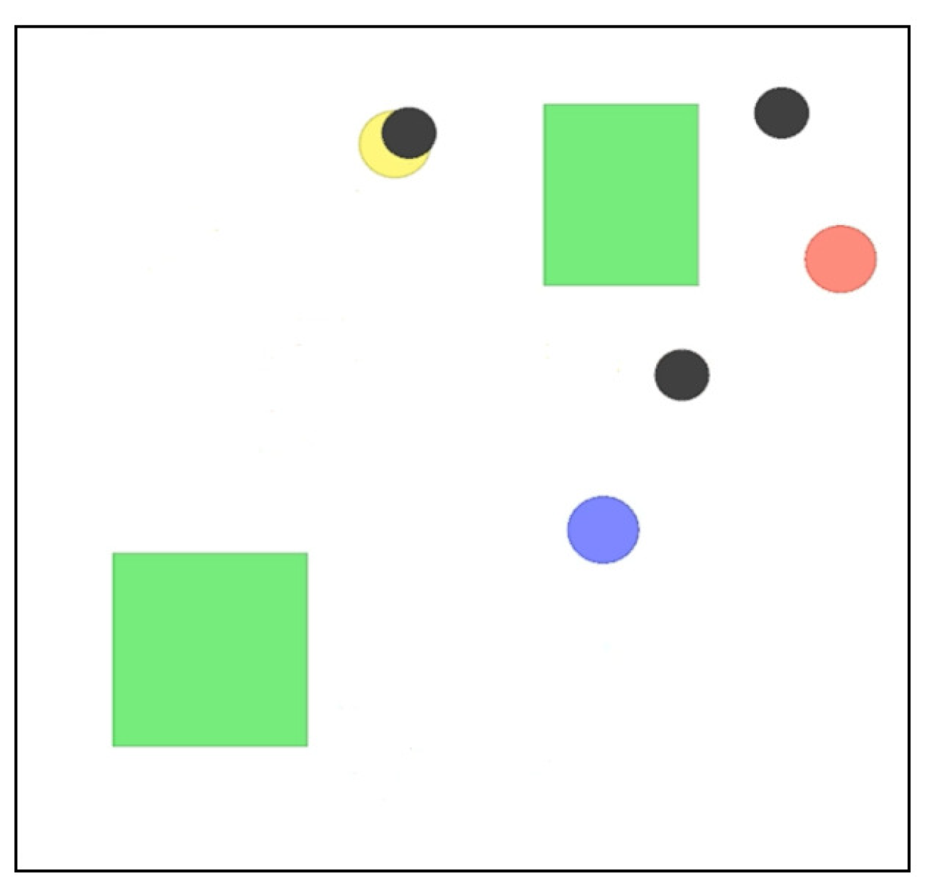
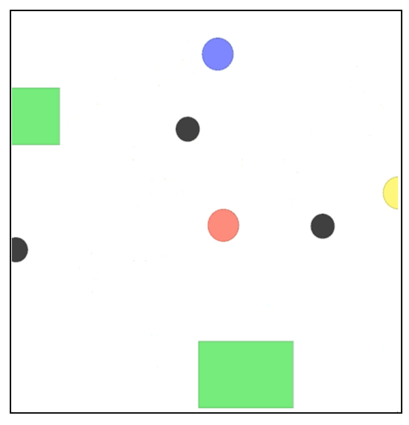
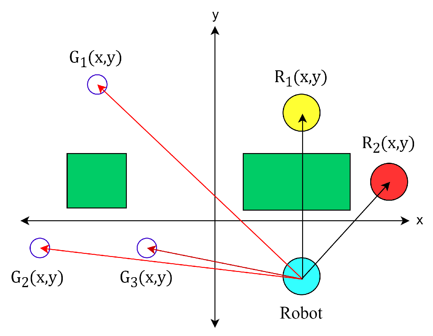
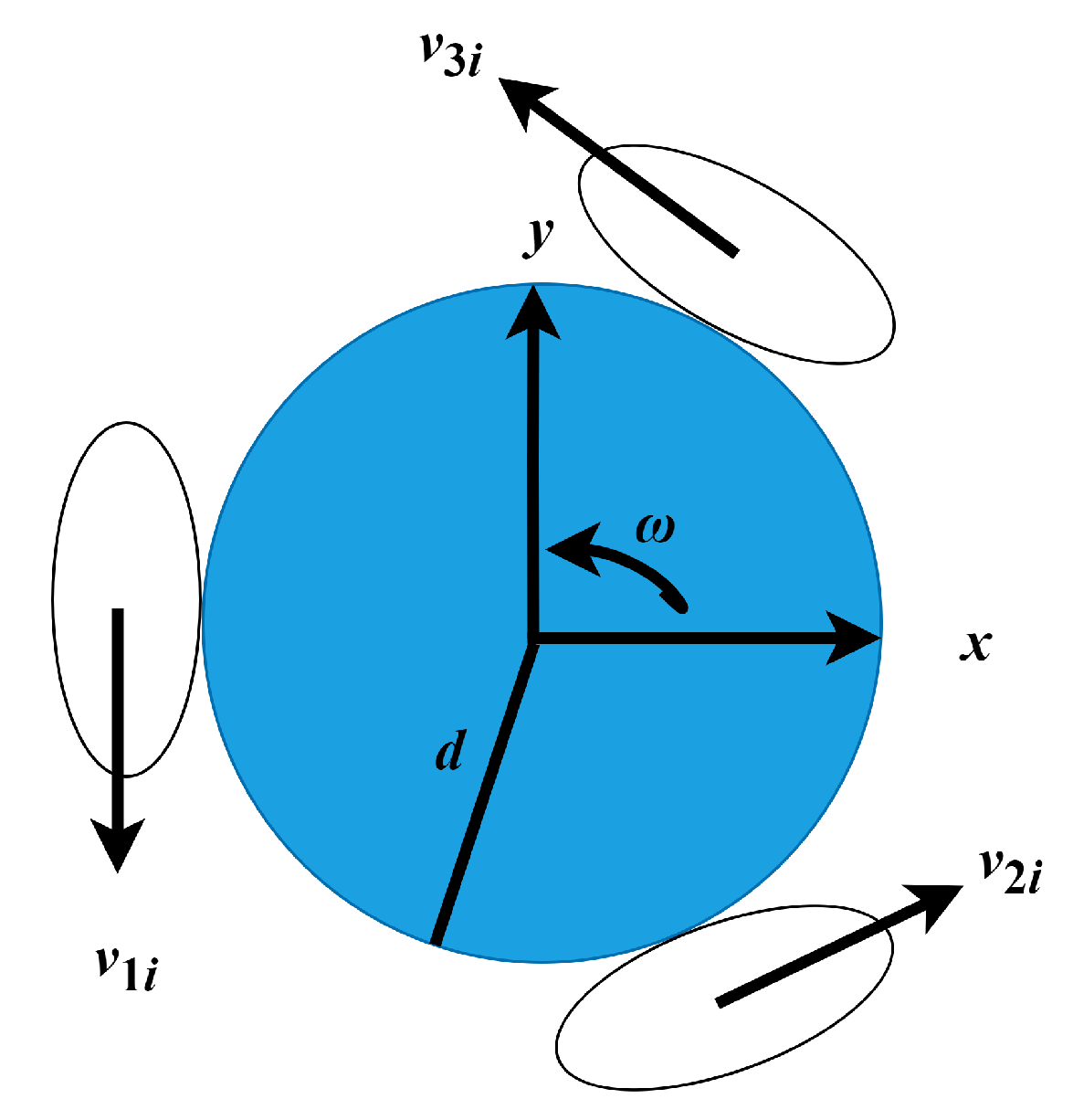
2. OpenAI Gym for a Simulated System

A formation change is required when it is necessary to change the arrangement of multiple agents. The environmental conditions affect the formation change, namely, avoiding obstacles, applying different sizes and shapes of tracks, and moving different sizes and shapes of transport objects. The actual experiment type adopted in this research was cooperative transportation with formation change with transport objects. The details of the initial formation and the formation change are shown in Figure 1 and Figure 2. The main theme in the scenario was moving transport objects (boxes) from one place to another place. After the robots finished moving one transport object by grasping the transport object, the robots moved to another transport object. The initial position in this scenario was around the first transport object (box), then the positions around the second transport object were the target points. This paper focused on the formation change from the initial position around the first transport object to the second transport object. The robot adopted in this research is shown in Figure 3, while the two suction cups used to grasp the transport object are shown in Figure 4. The number of agents was three robots, consisting of yellow, red, and blue robots. The number of transport objects was two, with small and medium-sized transport objects with dimensions of 580 mm × 430 mm and 850 mm × 430 mm. At the same time, the distance between the static obstacles was 900 mm. The size of the cooperative transportation area was 4 m × 3 m. The scenario of the formation change was as follows: the robots put down the medium transport object and then changed their formation to prepare to transport the small transport object. Each robot moved to reach the target point considering the other robots’ positions. Two cameras were attached to the wall at a height of 2700 mm. The distance between the cameras was 1000 mm. The agents used in this research were omnidirectional robots, as shown in Figure 3. Each robot consisted of a Raspberry Pi, Arduino Mega, Arduino 328, IMU, motor, and encoder.

The objective of the simulation experiment was to examine all of the components in the actual experiment so that the simulation experiment result will be as close to the actual cooperative transportation experiment. The simulation was applied in this research using OpenAI Gym, which is a Python library [19,20,21]. OpenAI Gym is a toolkit especially built for reinforcement learning research. OpenAI Gym has powerful features, such as providing the environment composition. The final performance and the amount of learning time can be examined in the reinforcement learning algorithm. The simulation was performed to investigate the performance of the algorithms before it was applied in the actual experiments. The OpenAI Gym was chosen for the simulation toolkit in this research. The Deep Dyna-Q algorithm was constructed in Python 3 and the simulation result was displayed in OpenAI Gym. The environment in the OpenAI Gym was set up according to the actual experiment system. The number of robots was three and the number of transport objects was two, with three sizes of transport objects.

OpenAI Gym with a random environment is shown in Figure 5 and Figure 6. The coordinate positions were extracted from the results of the web camera capture. The size of each robot point was 80 mm and the diameter of the target point was 60 mm. The initial positions of the robots represent the start positions of the robots, shown by the yellow, red, and blue circles, while the target positions are the target set points shown by the black circles. In the learning process, the size and positions of the transport objects were random, while the actual sizes of the transport objects were 580 mm × 430 mm (small), 850 mm × 430 mm (medium), and 870 mm × 575 mm (big). All of the coordinate readings were based on the web camera measurement.

3. Configuration of Deep Dyna-Q for Formation Change

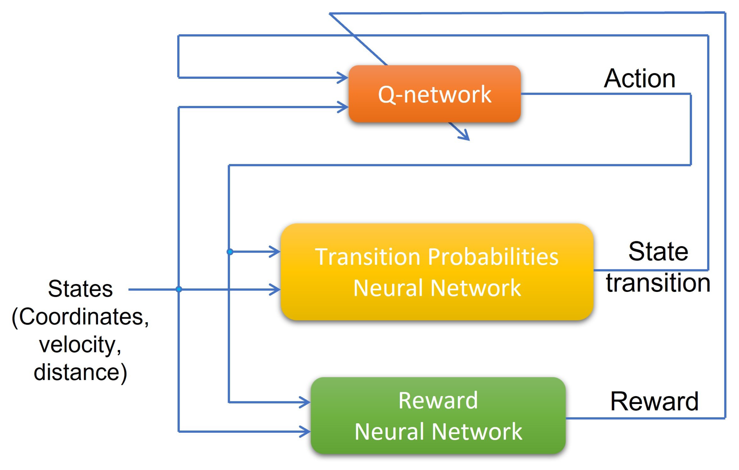
The proposed method challenged the issue of reinforcement learning in formation changes which has a long learning time. In recent research, the MADDPG algorithm showed effectiveness in a formation change system [15,20] compared to other methods such as DDPG (deep deterministic policy gradient) and actor–critic. Nevertheless, the MADDPG algorithm is a model-free learning method, in contrast, formation control is a complex system which needs long learning times. Training of neural networks is required for model-based approaches to improve the learning time. The Deep Dyna-Q is popularly used for model-based learning in formation change systems. A recent study [22] with Deep Dyna-Q in a formation change application had low accuracy for the formation achievement rate with an 80% success rate without an obstacle layout and 74% with an obstacle layout. Regarding the low accuracy, tuning the algorithm is needed. This research designed a system with the neural network (NN) applied to the formation change using Deep Dyna-Q.

3.1. Deep Dyna-Q

In model-free learning, such as MADDPG, the agent uses actual environmental samples and never uses the generated prediction of the next state and the next reward. In contrast, model-based learning uses the model’s predictions of the next state and the next reward in order to calculate the optimal actions. An approximation model estimates the transition probability and reward from the state and the reward obtained by the agent. Since the state and reward can be predicted, the number of samples is reduced and the learning time is improved.

Deep Dyna-Q is a model-based algorithm and the neural network construction of Deep Dyna-Q is shown in Figure 7 adapted from [22]. The Q-network denotes the neural networks in DQN, the transition probabilities neural network denotes the transition probability function in the approximate model, and the reward neural network denotes the neural network of the reward function in the approximate model.

In a Q-network, the input is the states, which are the coordinates, velocity, and distance value, while the output from a Q-network is an action, namely, the acceleration vector of the agents. In a Q-network, the value is updated by the Q-table, using (1) [23].

$$Q(s,a)=Q(s,a)+\alpha (r+\gamma \underset{a^{\prime }}{max}Q(s^{\prime },a^{\prime })-Q(s,a)),$$

(1)

where $\alpha$, r, and $\gamma$, are the learning rate, the reward, and the discount rate, respectively. $Q(s,a)$ is the Q value stored in the table, and $Q(s^{\prime },a^{\prime })$ is the maximum Q value in the destination state. The robot acts to select the best value in the destination state and learns to reduce the error in the updated equation. In this study, the tuning of the Deep Dyna-Q algorithm varied the parameter of the discount rate and the learning rate.

The discount rate has a role as a regulariser in reinforcement learning. Using the discount factor, rewards are gradually scaled down after each step so that the total sum remains bounded. This study investigated the impact of the discount rate on formation control and multi-agent systems. The standard treatment of the reinforcement learning problem is the Markov decision process, which uses a discount factor between 0 and 1, which reduces the present value of future rewards exponentially. The discount rate varied between about 0.85 and 0.95 in this paper. The discount rate in Deep Dyna-Q is fundamental, so studies have focused on the discount rate calculations [16,17,18]. The discount rate in Deep Dyna-Q maximises the value function of the Markov decision process (MDP). The discount rate values future rewards by an exponential scheme that leads to guaranteed theoretical convergence of the Bellman equation [16,17,18].

The model’s learning rate determined by how quickly it picks up new information. The learning rate is set between 0 and 1. Setting it to 0 means that the Q-value is never updated; therefore, there is no learning. The learning is rapid when a high value is set, such as 0.9. Extremely high learning rates will provide weight updates that are too large, which will cause the model’s performance to fluctuate over training epochs. It is typically impossible to determine the ideal learning rate in advance [24]. Trial and error are required to determine the optimal parameters for formation achievement improvement. The learning rate was varied between 0.01 and 0.08 in this study, following reference [23], and the impact on formation control was investigated.

The probability function was based on a Markov decision process (MDP), which is shown in (2). From the transition probability function, a transition probability distribution is obtained from the current state to the state several steps ahead, where s_t is the current state, s${}_{t+1}$ is the next state, a_t is the action taken from s_t, p is the transition probability, and T is the transition probability function.

$$T=p\left(s_{t+1}\right|s_t,a_t)$$

(2)

In the transition probabilities neural network, the NN consisted of 16 neurons in the input layer, 16 neurons in the hidden layer, and five states to be observed in two output layers (5 × 2 neurons). The two output layers were average and deviation. In the reward neural network, the NNs had three layers: the input layer was 16 neurons, the hidden layer was 16 neurons, and the output layer was 1 neuron. The input vector of the NNs was the same as the Q-network neural network, while the output was the reward. The reward was calculated based on the reward function. In the reward function, a value proportional to the distance was calculated as a negative value which measured the distance between a robot and the target point. If there was a collision between agents, the negative reward of −1 was added, while if there was a collision between the agent and the transport object, the negative reward of −1 was added. The total reward of each agent was the sum of the rewards of value distance, collisions between agents, and collisions between agents and target points. The more positive the reward was the better the performance of the agent.

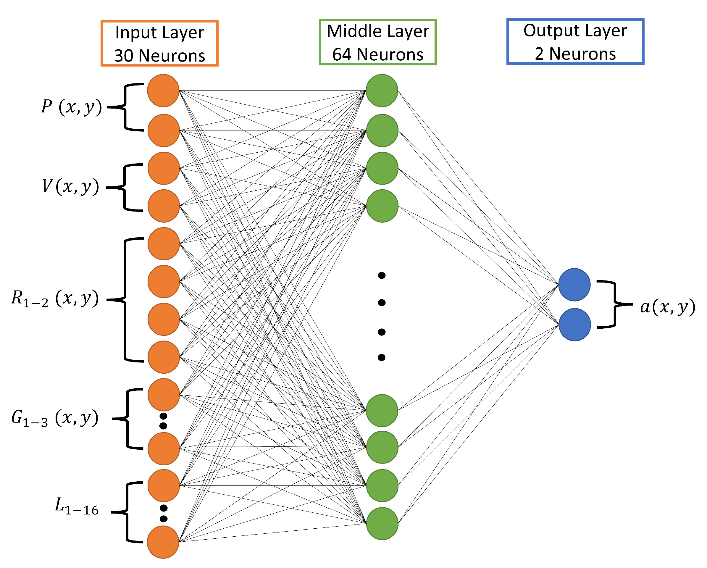
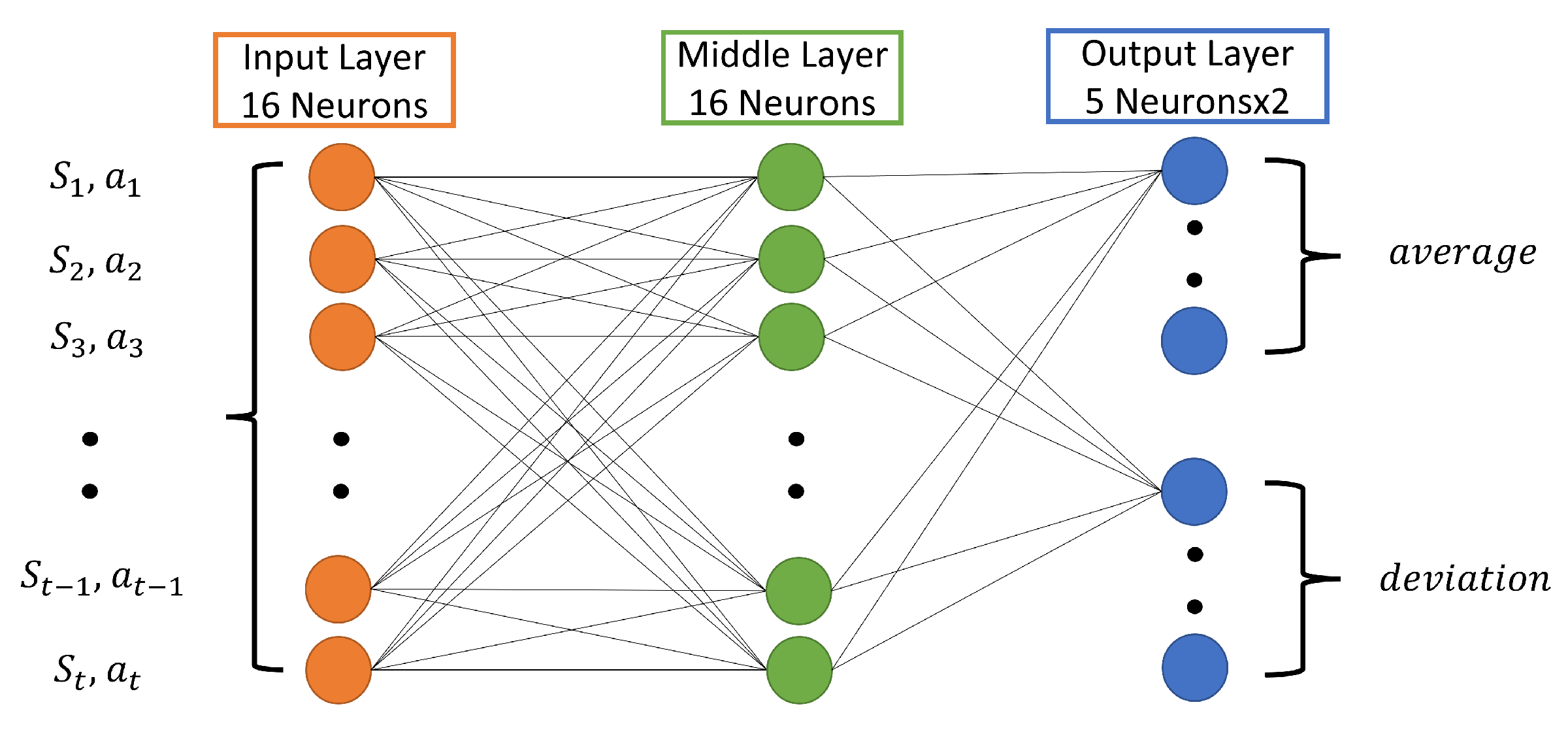
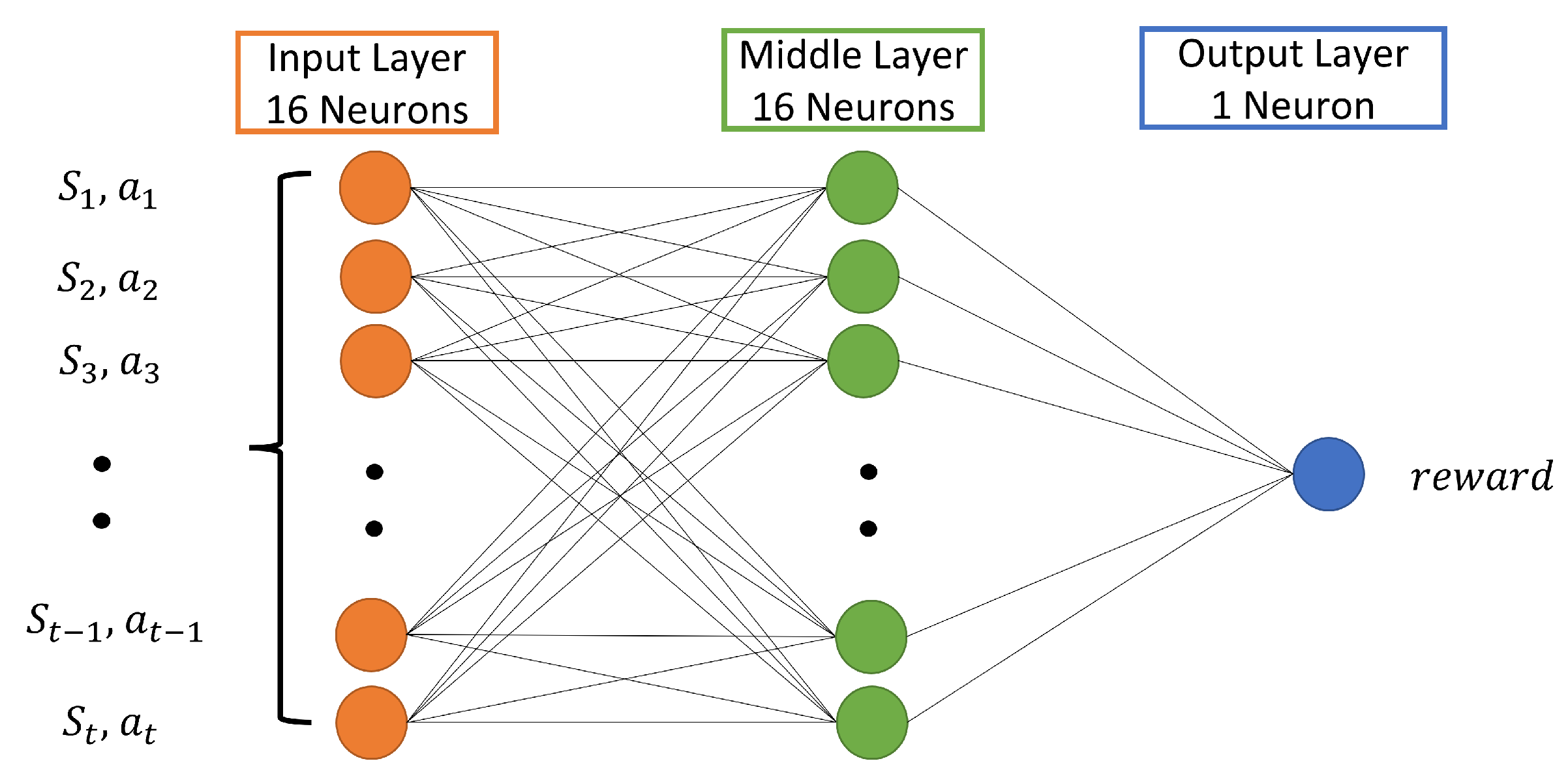
3.2. Learning Method and Neural Network Construction

The comprehensive investigation in the simulation experiment consisted of the formation change achievement rate, collision number among agents, and collision number between agents and transport objects. In order to act appropriately in any formation changes, versatile NNs were needed. The neural networks were trained in random environments to learn any conditions of the robots and transport objects. In the robot environments, each robot’s initial and goal positions were changed randomly. Each robot did not have one definite target point, but each could reach all target points based on the conditions of the robot, transport objects, and other robots. The parameters that varied in the transport objects were the size, ratio, and position of each transport object.

The Q-network neural network design is shown in Figure 8. This explains the NN algorithm used to determine the acceleration vector of the robots. The NN had three layers: the input layer had 30 neurons, the hidden layer had 64 neurons, and the output layer had two neurons. The input vector of the NN was P(x,y), V(x,y), G_1–3(x,y), R_1–2(x,y), L_1–16. P(x,y) and V(x,y) denote the position and velocity of the robots, respectively.

There were three goals available that the robot could reach based on the relative position to the target point and the positions of the other two robots. Figure 9 represents the definition of them. G_1–3(x,y) and R_1–2(x,y) denote the relative coordinates of the target points and other robots.

L_1–16 was the input of the virtual lidar sensors line used to measure the distances between the robots and transport objects, as shown in Figure 10. Every single lidar sensor line was calculated as one lidar (L_i). As Figure 10 shows, three lidar lines detect the transport object.

Figure 11 shows the description of the transition probabilities neural network. The input was the state and the action was the output from the Q-network neural network. The outputs of the transition probabilities neural network were the average and deviation. The output from the probabilities neural network was used as input for the Q-network neural network. The description of the reward neural network is shown in Figure 12. The inputs were the state and the output was the action from the Q-network neural network. The output from the reward neural network was the reward.

4. Simulation Results

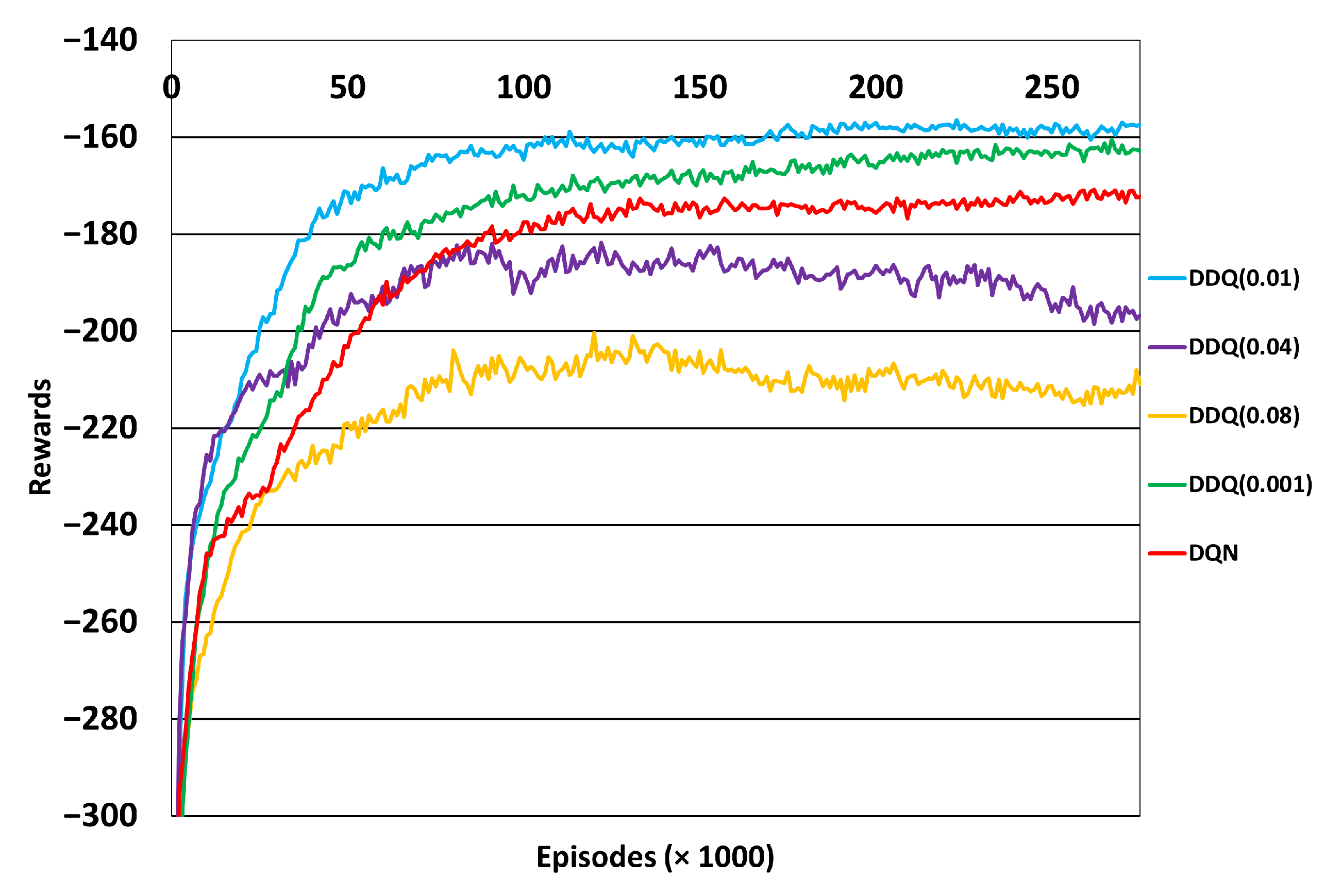
4.1. Transition of Rewards

The rewards were calculated based on the reward function. The comparison of transition rewards during learning in DQN and various learning rates of Deep Dyna-Q is shown in Figure 13. The various learning rates are presented to evaluate the transition reward for each value [14,23,25,26]. The horizontal axis represents the scenarios in thousands (×1000), while the vertical axis shows the reward values. The reward value presented is the total reward of the three agents. As seen in Figure 13, the reward transition comparisons are for DQN and DDQ with learning rate values of 0.001, 0.01, 0.04, and 0.08, as detailed in Section 4.3. A more positive reward indicates a better performance of the agent. A more positive reward shows that the distance between the goal and the agents was closer, and fewer collisions occurred. These rewards correlated to the formation change achievement rate, collision number among agents, and collision number between agents and transport objects. The agents’ performance in the initial few episodes was similar, after that the performance improved. The DQN obtained a maximum of about −170 rewards in around 130,000 episodes. While other variations in DDQ could achieve the −170 reward in 58,000 and 98,000 episodes for DDQ (0.01) and DDQ (0.001), respectively. On the other hand, DDQ (0.04) and DDQ (0.08) could only reach maximum reward values of −197 and −207 instead of the value of −170 achieved by DQN. DDQ (0.01) obtained the highest reward value, about −160 in 100,000 episodes. For a summary comparison, the DQN obtained the maximum −170 reward in about 130,000 episodes while the DDQ (0.01) could achieve this value in 58,000 episodes and achieved a maximum −160 reward.

4.2. Discount Rate Tuning

The discount rate is one of the hyperparameters used to update the Q-table in Deep Dyna-Q. The discount rate will affect the Q-value in order to obtain the best value to determine each robot’s action. The discount rates compared in this research were 0.85, 0.9, and 0.95, according to recent research about the algorithm’s application [14,23,25,26].

Table 1. Evaluation of learning with different discount rates.

Evaluation	0.85	0.9	0.95
Formation change achievement rate	100%	100%	100%
Collision number among agents	0	0	0
Collision number between agents and transport objects	1.35	1.01	1.23

displays an evaluation of the learning for values of 0.85, 0.9, and 0.95. The formation change achievement rate meant all the robots could reach the target points. The collision number among agents shows the average number of collisions among the agents per episode. At the same time, the collision number between agents and transport objects indicates the average collision number among agents and transport objects. In Table 1, the three discount rates of 0.85, 0.9, and 0.95 have a 100% formation change achievement rate. This means that with all three discount rate values, the robots could successfully reach all the target points. In the collision number among agents, the percentage 0% was reached by all three values. On the other hand, the collision numbers between agents and transport objects for discount rate values of 0.85, 0.9, and 0.95 were 1.35, 1.01, and 1.23, respectively. Regarding this result, the value of 0.9 had the best result because it had the lowest point among the three values. Every episode consisted of 35 steps and in every episode, there were about 0–4 collisions. This value was the average collisions per episode in 100 episodes.

Figure 14, Figure 15 and Figure 16 show the trajectories of Deep Dyna-Q with discount rates of 0.85, 0.9, and 0.95, respectively. Square shapes mark the initial point of each robot, while the circle shapes mark the target points. The target points did not specifically define a particular robot, the robots could coordinate and reach the most efficient target point. Figure 14 and Figure 15 indicate smoother trajectories than the trajectory in Figure 16. The yellow robot generally could reach the target point almost in the same way for all various discount rate values. Different trajectories were taken by the blue and red robots.

4.3. Learning Rate Tuning

In addition to the discount rate, the learning rate has an important role in the Deep Dyna-Q calculation.

Table 2. Evaluation of learning with different learning rates.

Evaluation	DDQ (0.001)	DDQ (0.01)	DDQ (0.04)	DDQ (0.08)	DQN
Formation change achievement rate	94%	100%	72%	10%	91%
Collision number among agents	0	0	0.76	0.92	0.06
Collision number between agents and transport objects	2.15	1.01	1.75	3.01	3.69

shows the evaluation of the learning with different learning rates. The compared learning rates were chosen by a review of the literature [14,23,25,26]. The learning value variations chosen were 0.001, 0.01, 0.04, and 0.08 for Deep Dyna-Q, and as a comparison the DQN analysis was added.

Based on Table 2, in the formation change achievement rate percentage evaluation, the learning rate value of 0.001 achieved a result of 94%, the 0.01 value achieved a 100% result, and the 0.04 value achieved a lower value of 72%. On the contrary, the 0.08 learning rate achieved only 10% for the formation achievement rate. In comparison, the DQN had a formation achievement rate of about 91%. These conditions specified the best performance order as DDQ (0.01), DDQ (0.001), DQN, DDQ (0.04), and DDQ (0.08). Furthermore, for the collision number among agents and collision number among agents and transport objects, the learning rate of 0.01 gave the best performance. The 0.01 learning rate had a 0 collision number among agents and a 1.01 collision number among agents and transport objects. For the last comparison, the collision number among agents and between the agents and transport objects were 0 and 2.15 for a 0.001 learning rate, 0.76 and 1.75 for a 0.04 learning rate, and 0.92 and 3.01 for a 0.08 learning rate. While DQN had values for the collision number among agents and collision number between agents and transport objects of 0.06 and 3.69, respectively. These values were the lowest performance among all of the algorithms. Figure 17, Figure 18, Figure 19 and Figure 20 indicate the trajectory of Deep Dyna-Q with 0.001, 0.01, 0.04, and 0.08 learning rate values.

According to Figure 17, Figure 18, Figure 19 and Figure 20, it can be seen that the yellow robot has almost the same trajectory. The yellow robot’s target point can be reached appropriately only with the learning rate 0.01 in Figure 18, while the target point is shifted with other learning rate values. Figure 19 and Figure 20 have almost the same trajectories.

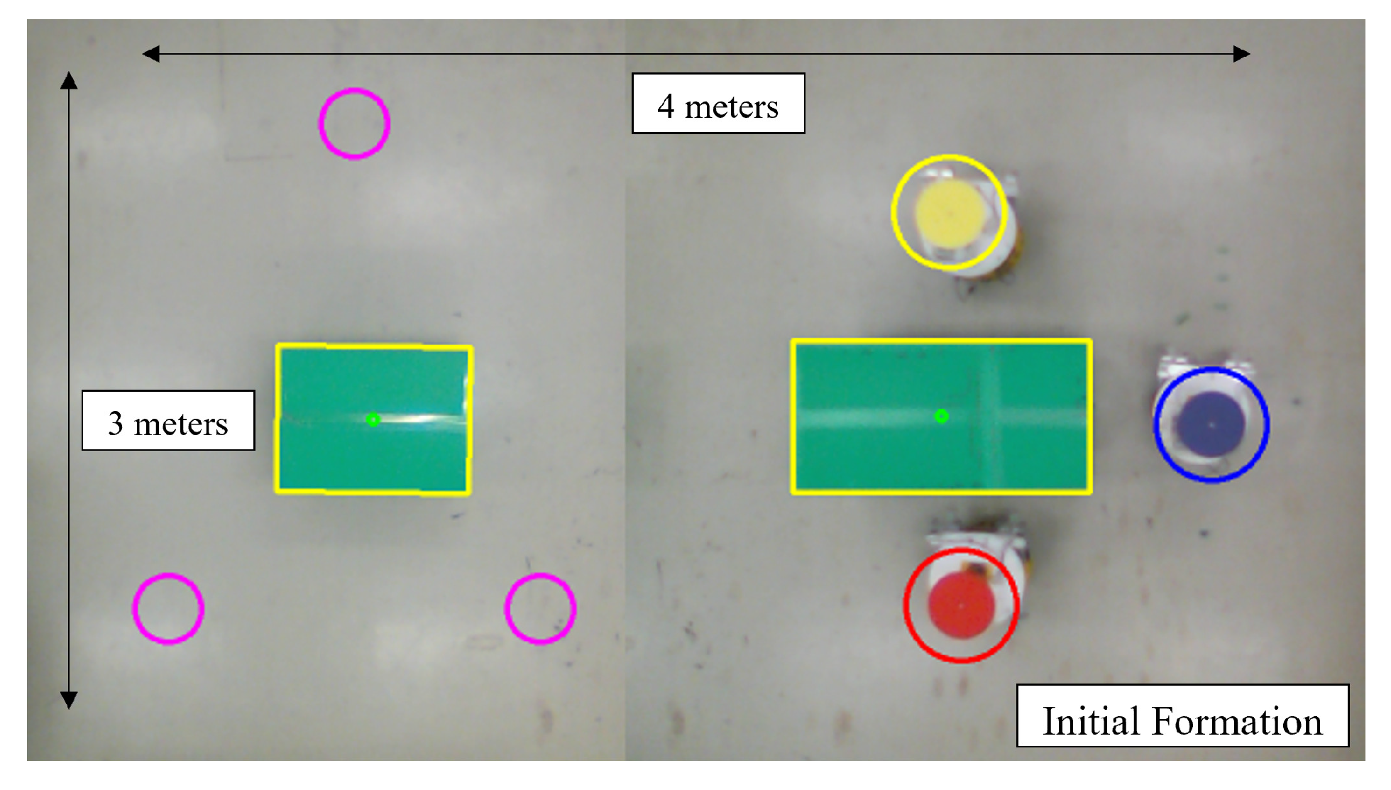
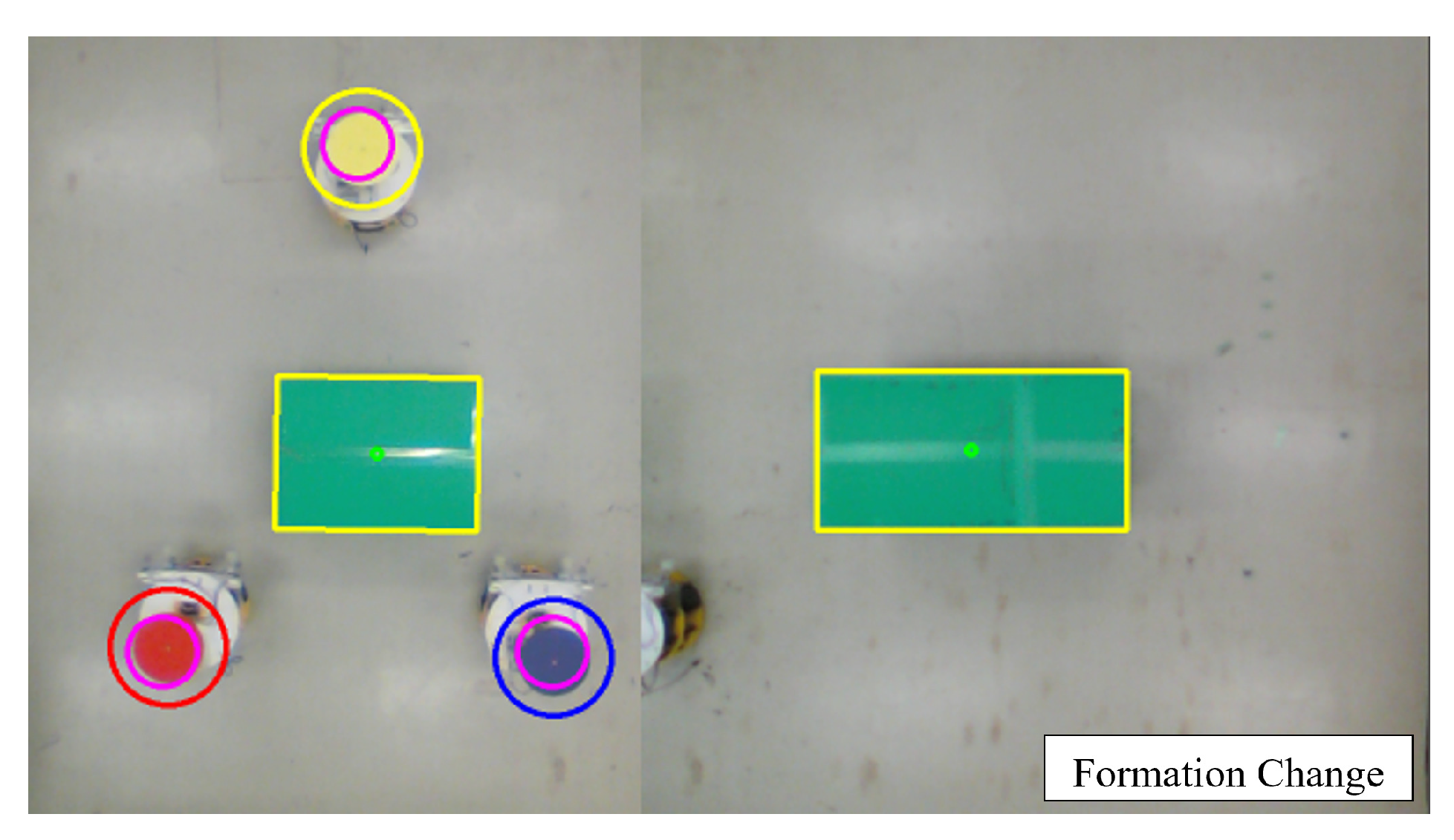
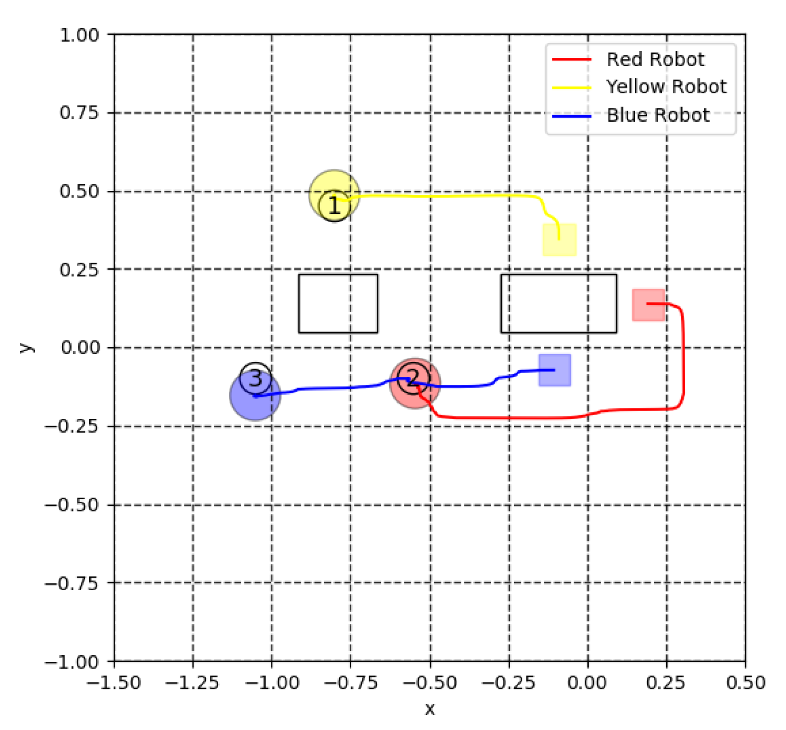
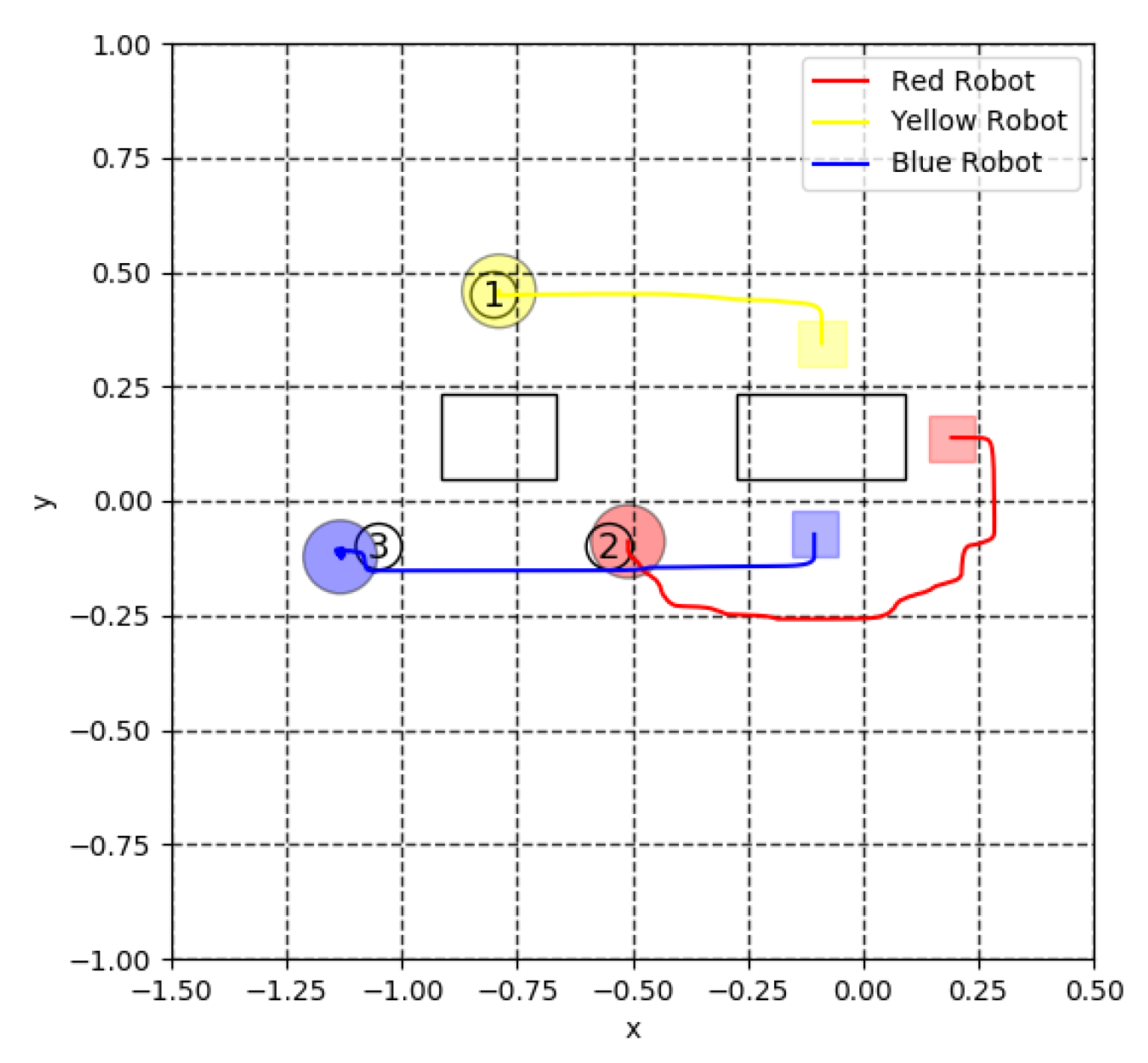
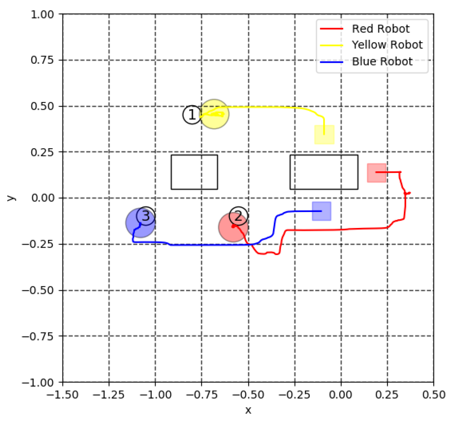
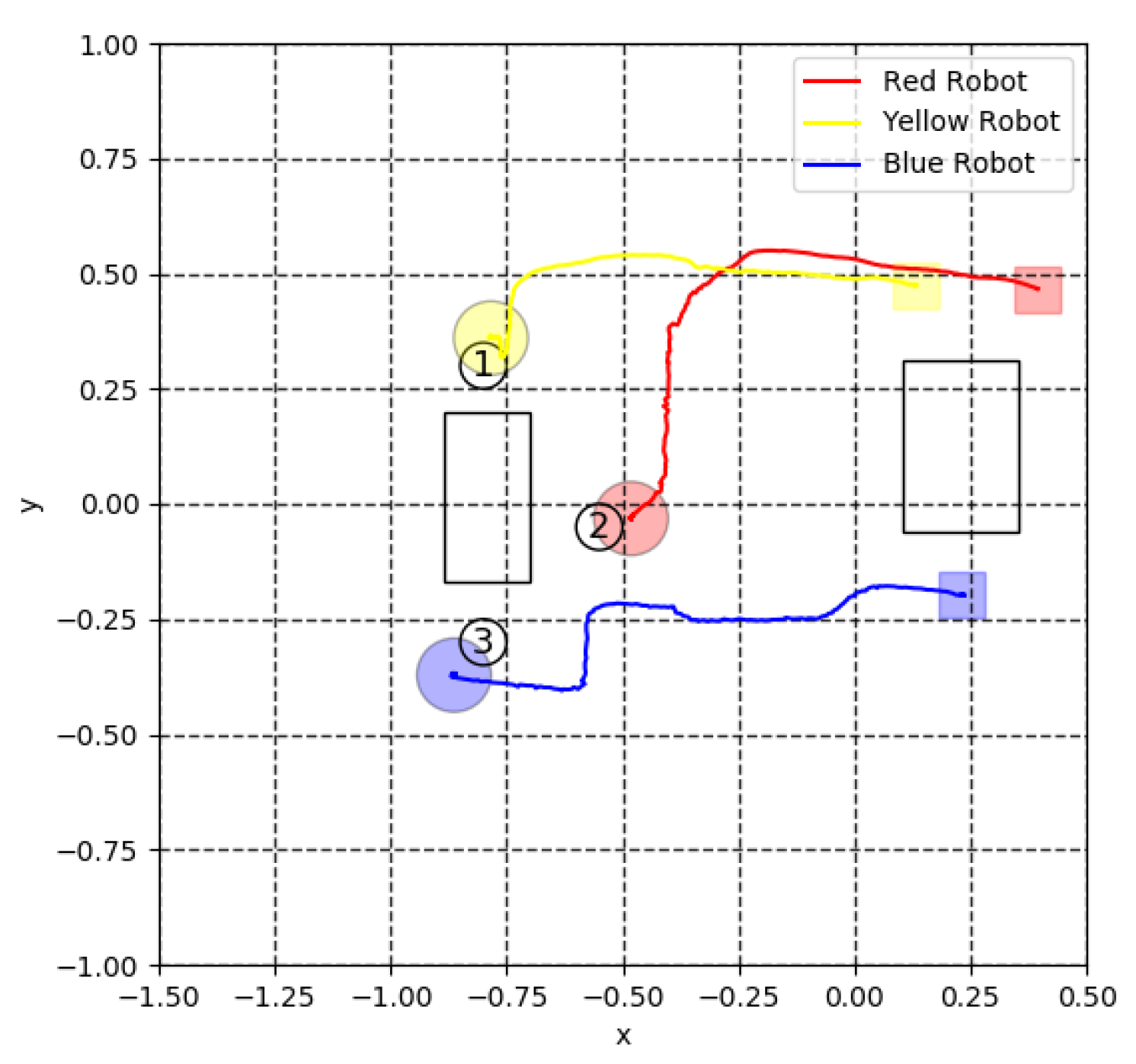
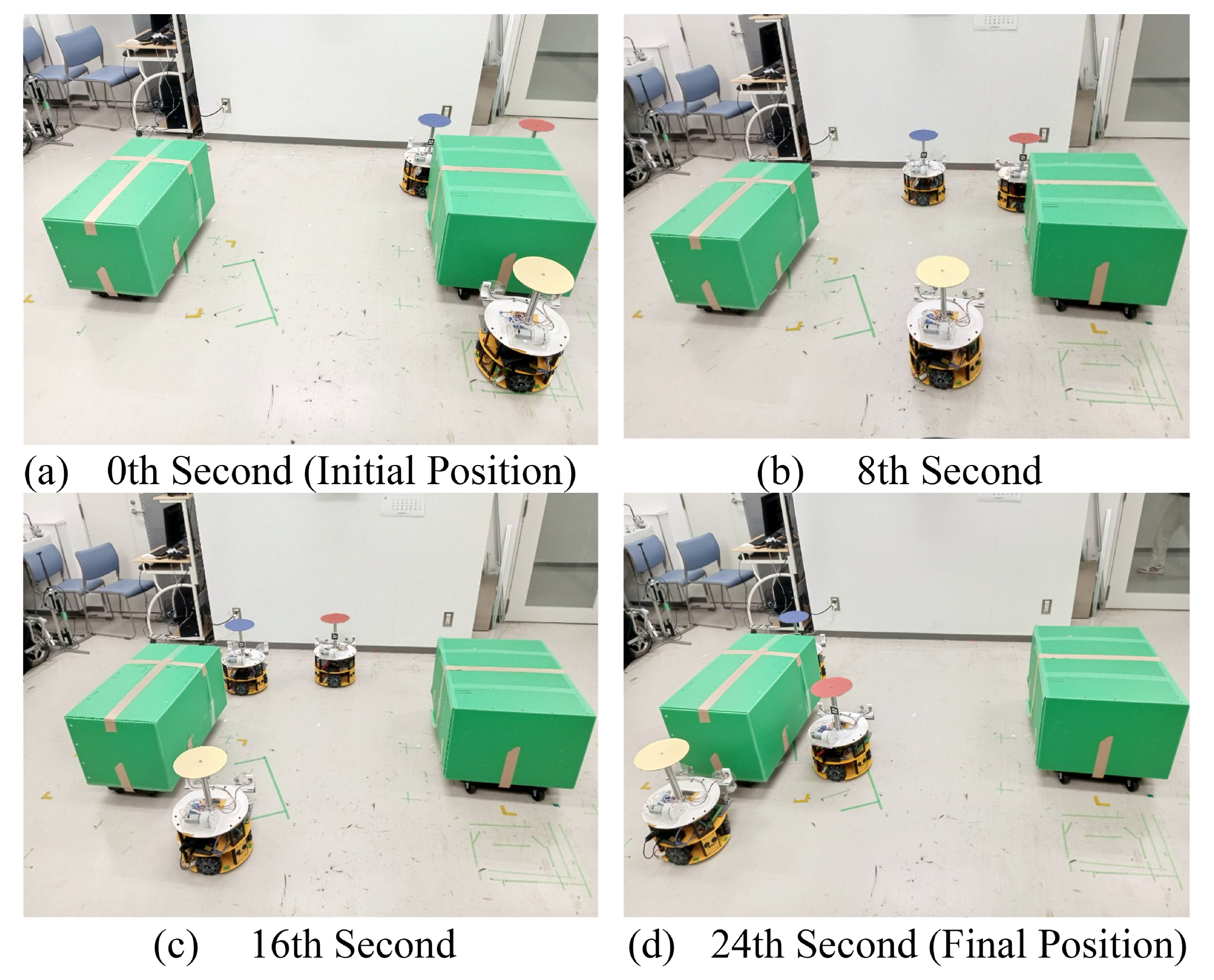
5. Experiment for Cooperative Transportation

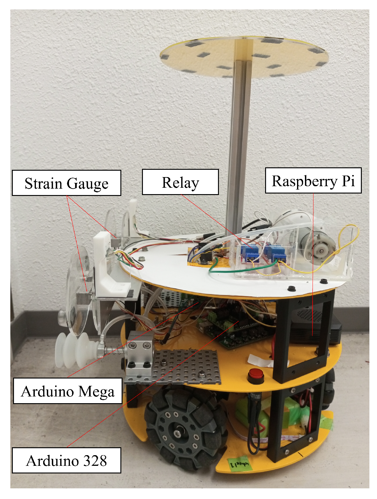
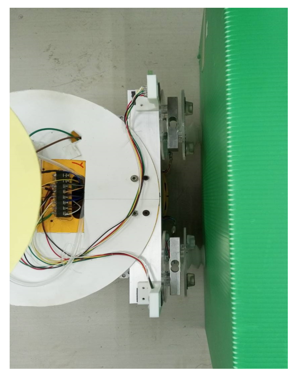
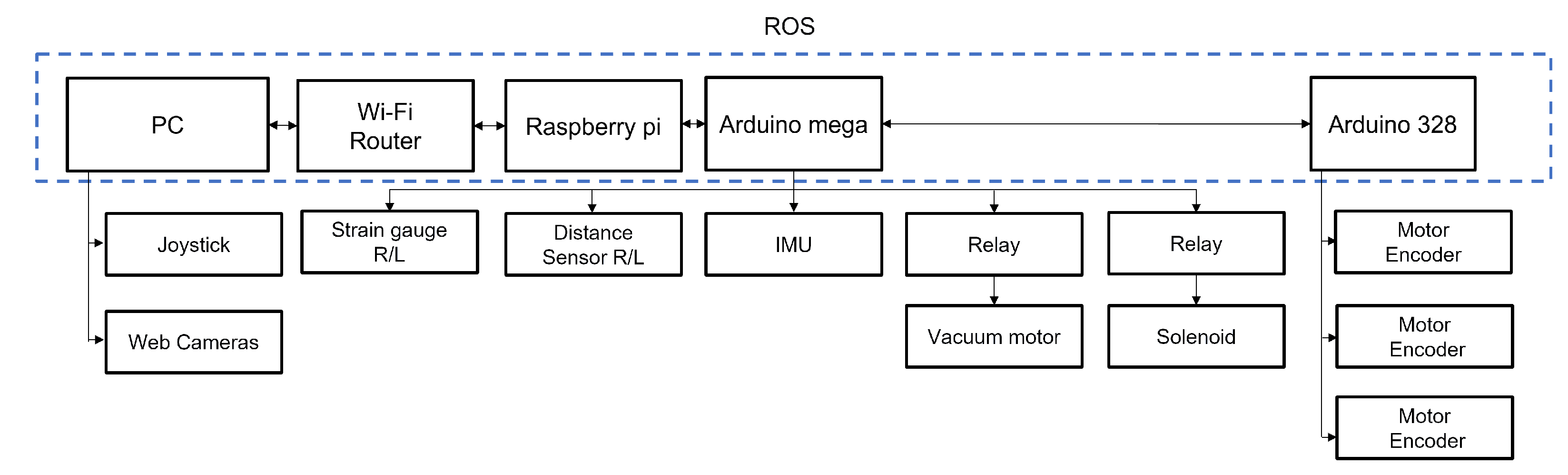
5.1. Robot Mechanism

The body coordinate system of the Nexus robot is shown in Figure 21. This body coordinate system was the basis of the robots’ movements. The movements of the robots were omnidirectional or holonomic movements. Each robot consisted of three omni wheels, which were freewheel rollers on perpendicular planes to their rotation axis. As a result of sliding in the parallel direction to the rotation axis, omnidirectional movement was attainable [27]. Where v_1i, v_2i, and v_3i are the velocities of each wheel on the ith robot. The parallel velocities of each robot in the x-axis and y-axis are denoted by v_iX and v_iY, respectively, and w_i is the angular velocity. The relationship between each robot’s velocity and the parallel velocity is denoted as follows:

$$\left[\begin{array}{c}{v}_{1i}\\ v_{2i}\\ v_{3i}\end{array}\right]=\left[\begin{array}{ccc}0& -1& d\\ -\frac{\sqrt{3}}{2}& \frac{1}{2}& d\\ \frac{\sqrt{3}}{2}& \frac{1}{2}& d\end{array}\right]\left[\begin{array}{c}{v}_{iX}\\ v_{iY}\\ w_i\end{array}\right]$$

The block diagram system of the robots is shown in Figure 22. The images captured by the web camera were processed on a personal computer (PC). The image result was used to present the position of each robot and transport objects. This position was fundamental to determining the robot’s direction and speed. A Wi-Fi router connected to the PC was used to communicate with the Raspberry Pi which works as the main processor in each robot. The Raspberry Pi connected to the Arduino Mega controlled the strain gauges, relays for the vacuum motor and solenoid, distance sensors, and inertial measurement unit (IMU). The number of strain gauges was two, with the function to measure how strongly the robots could hold the object. The vacuum motor and solenoid had roles in controlling the suction cups when holding the object. Moreover, the Arduino Mega was connected to Arduino 328. Arduino 328 was responsible for managing the motor movements by controlling the three motor encoders.

An ROS (robot operating system) was used for the actual experiments. The actual experiments used ROS1 and ROS2 to construct the system. The PC connection to the Raspberry Pi used the ROS2 connection through the wifi router. The Raspberry Pi used ROS2, while the Arduino Mega used ROS1. Some packages were not available in ROS2, so the Arduino Mega used ROS1. The Arduino Mega was connected to the Raspberry Pi using an ROS bridge for connecting between ROS2 and ROS1. The PC gave the commands to the robots in the form of the velocity of each robot. The robots’ positions and the transport objects’ were sent to the PC using ceiling camera detection so that the central processor could calculate the distance and position of the target positions and give the velocity to each robot in real-time. Thereafter, the velocity of each wheel was calculated in the Arduino.

The robot hardware had a limitation in its velocity from the neural network so that the robot’s movement should be restricted. When the robot’s movement was not restricted, the robot could not move according to the neural network’s velocity command. On the other hand, the restriction could not be given immediately to avoid the saturation in the velocity. As the solution, a low pass filter was given to restrict the velocity of the robots so that the velocity of the robots could be restricted without any saturation. The low pass filter was applied both in the simulation and actual experiment.

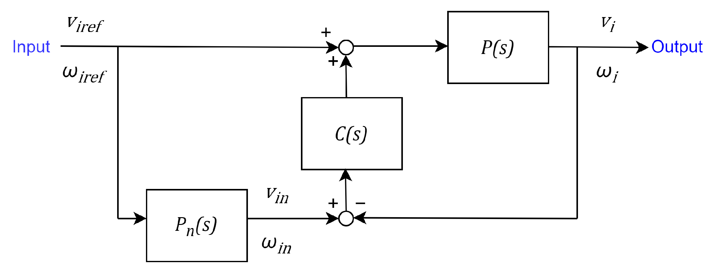
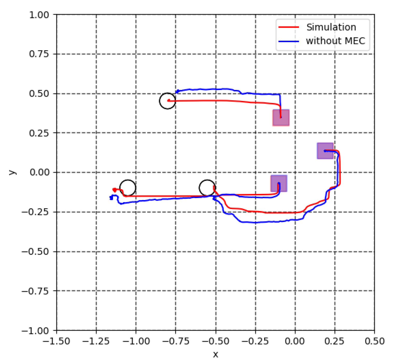
5.2. Model Error Compensator (MEC)

In the actual experiment, the investigation contained the application of an MEC to control the agents’ movement and trajectory analysis between the simulation and actual experiments. Normally transfer learning or fine-tuning is required to fit environmental change. On the other hand, robust control was applied to suppress the disturbance. It was useful to design a robust controller MEC to reduce the burden of retraining. In the actual experiment, the controller of the robots’ movement used a model error compensator (MEC) [28]. The controller was used to minimise the model error in the system. Each robot had its own controller with an MEC. The block diagram of the control system is shown in Figure 23. The controller was implemented in Arduino 328, which controlled each robot’s movement using a motor encoder.

P(s) is the actual plant, P_n(s) is the nominal model, and C(s) is the compensator. The robot inputs are w_iref and v_iref. Where w_iref is the angular velocity of the ith robot. The velocity in the x-axis and y-axis for each robot is denoted by (3).

$$v_{iref}={[v_{irefX},v_{irefY}]}^T.$$

(3)

v_in and w_in are the output from P_n(s). The MEC was designed to compensate for the model error between the actual plant P(s) and nominal model P_n(s) as follows (4):

$$▵P=P\left(s\right)-P_n\left(s\right).$$

(4)

The $P_n$(s) with a time constant of 0.2 is represented as follows:

$$\left[\begin{array}{ccc}{\displaystyle \frac{1}{0.2s+1}}& 0& 0\\ 0& {\displaystyle \frac{1}{0.2s+1}}& 0\\ 0& 0& {\displaystyle \frac{1}{0.2s+1}}\end{array}\right]$$

The compensator C(s) of the MEC was designed with parameters Kp, Ki, and Kd as 1.3, 5.5, and 0, respectively. The compensated outputs are w_i and v_i. The effectiveness of the MEC in the robots was evaluated by comparing the application of the MEC in the robots to not applying the MEC.

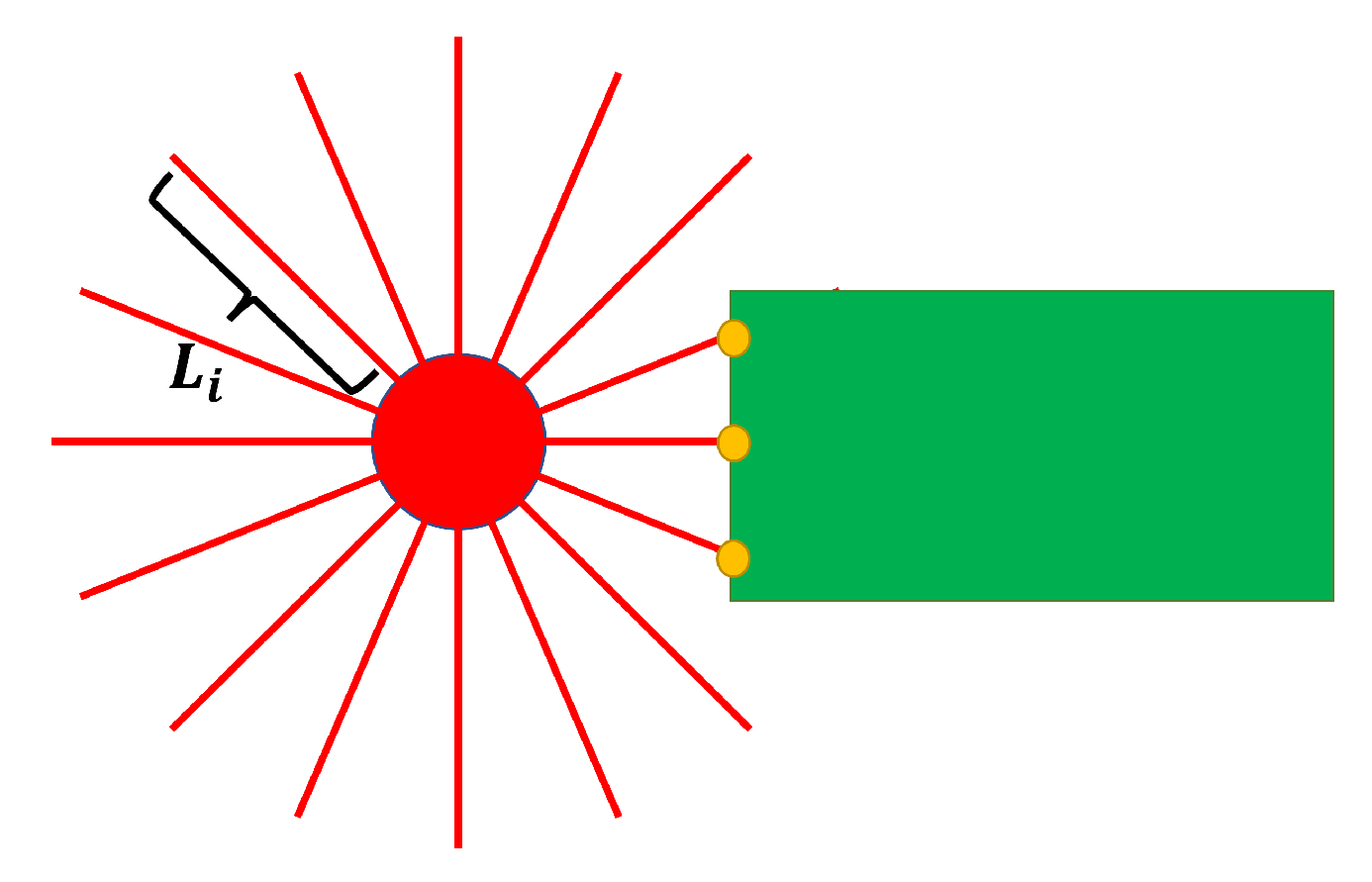
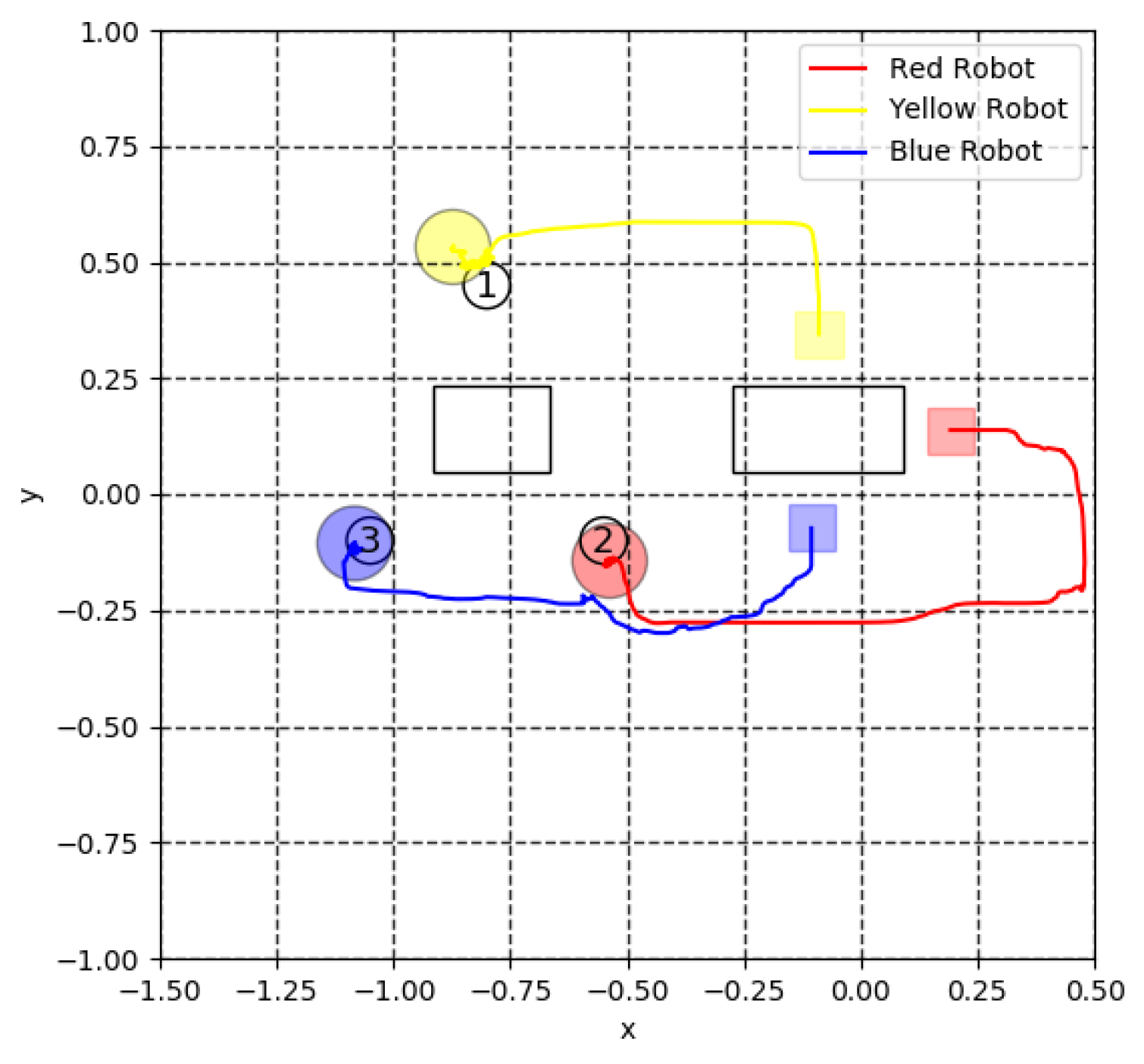
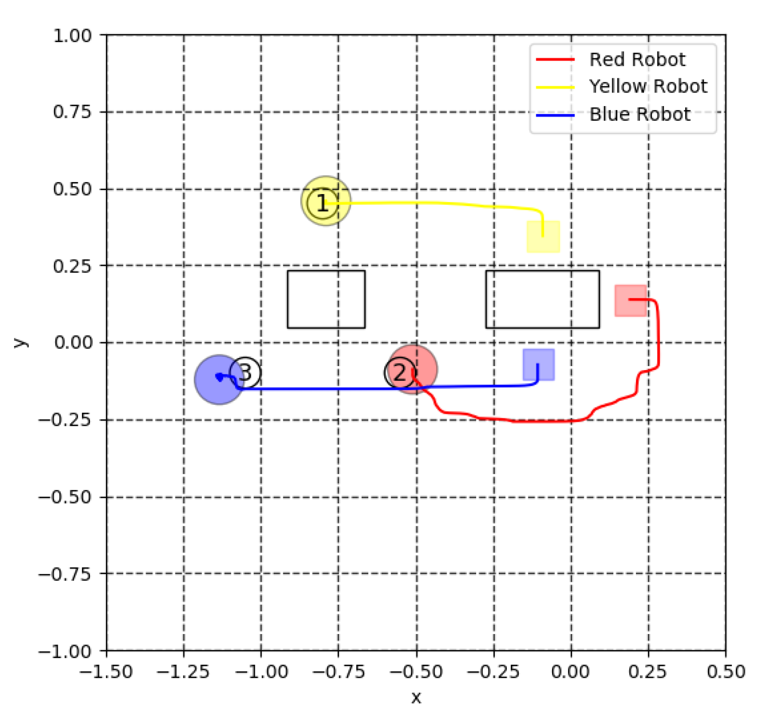
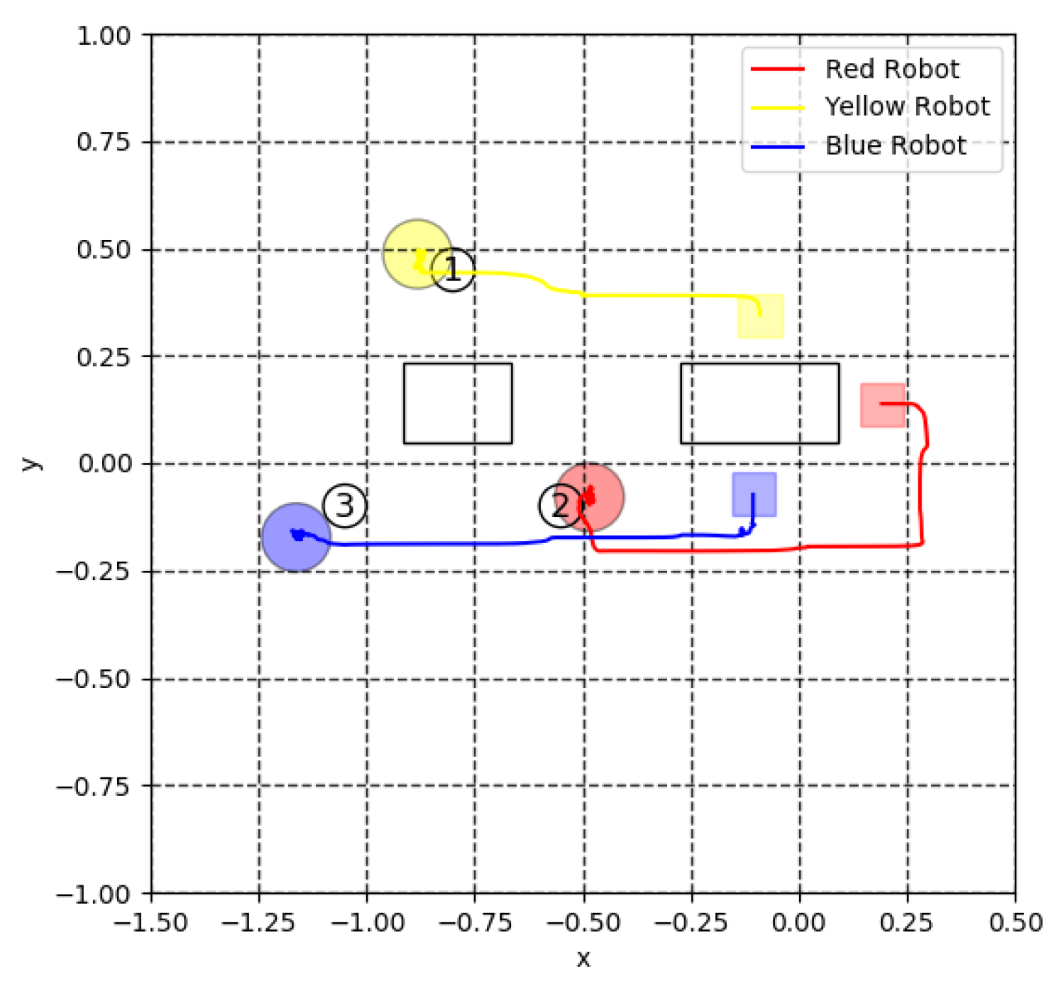
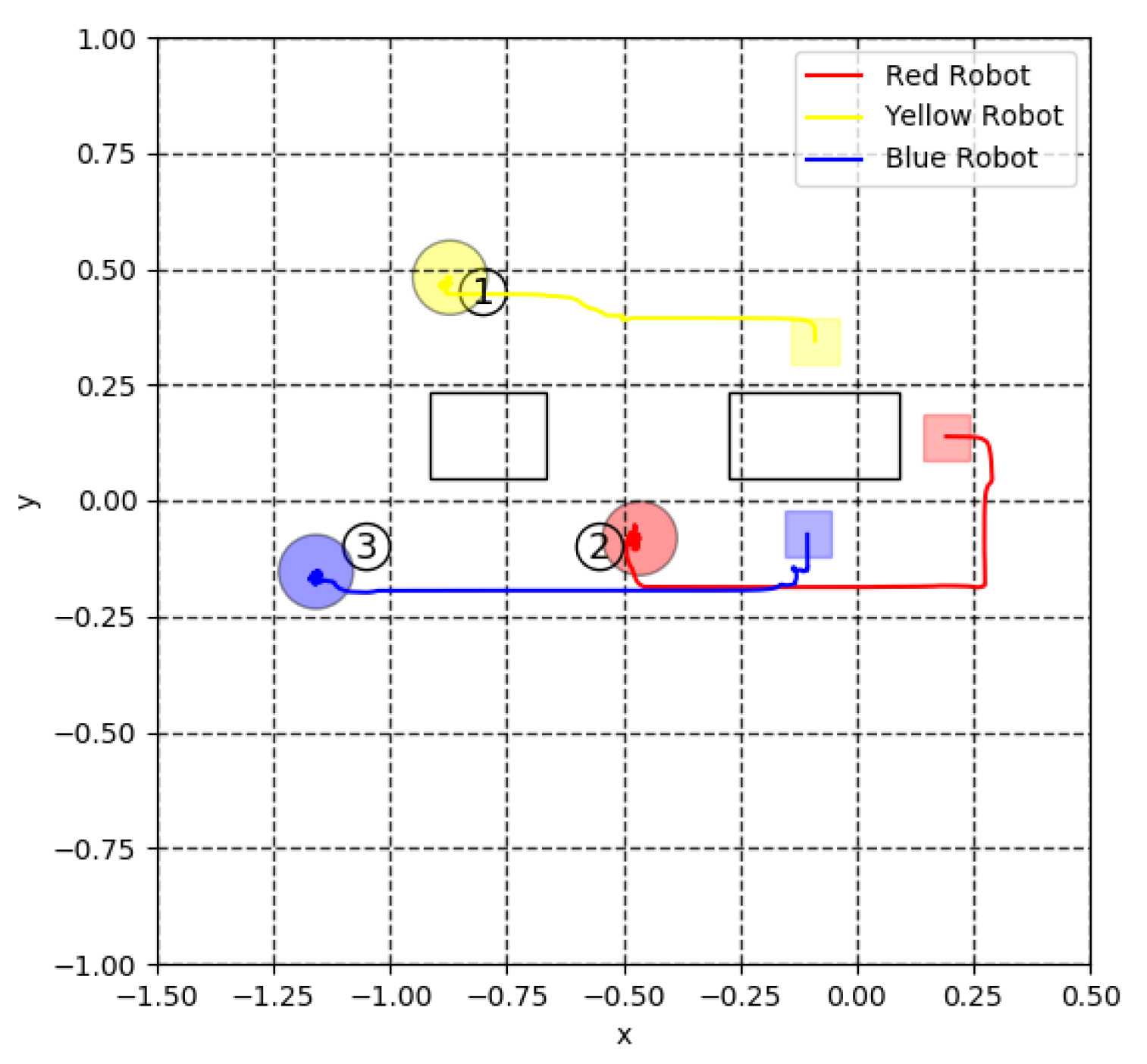
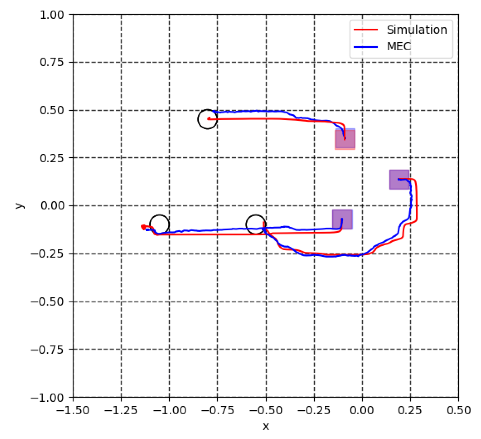
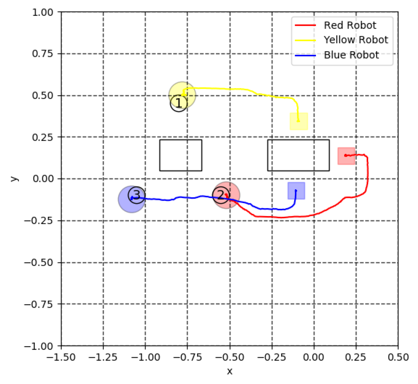
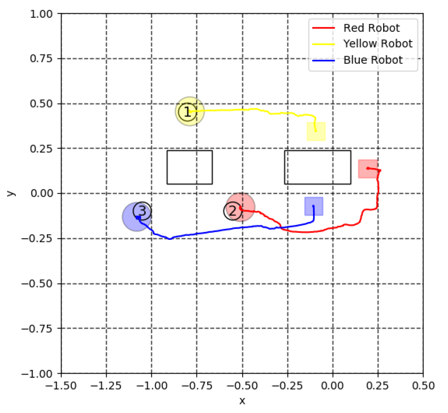
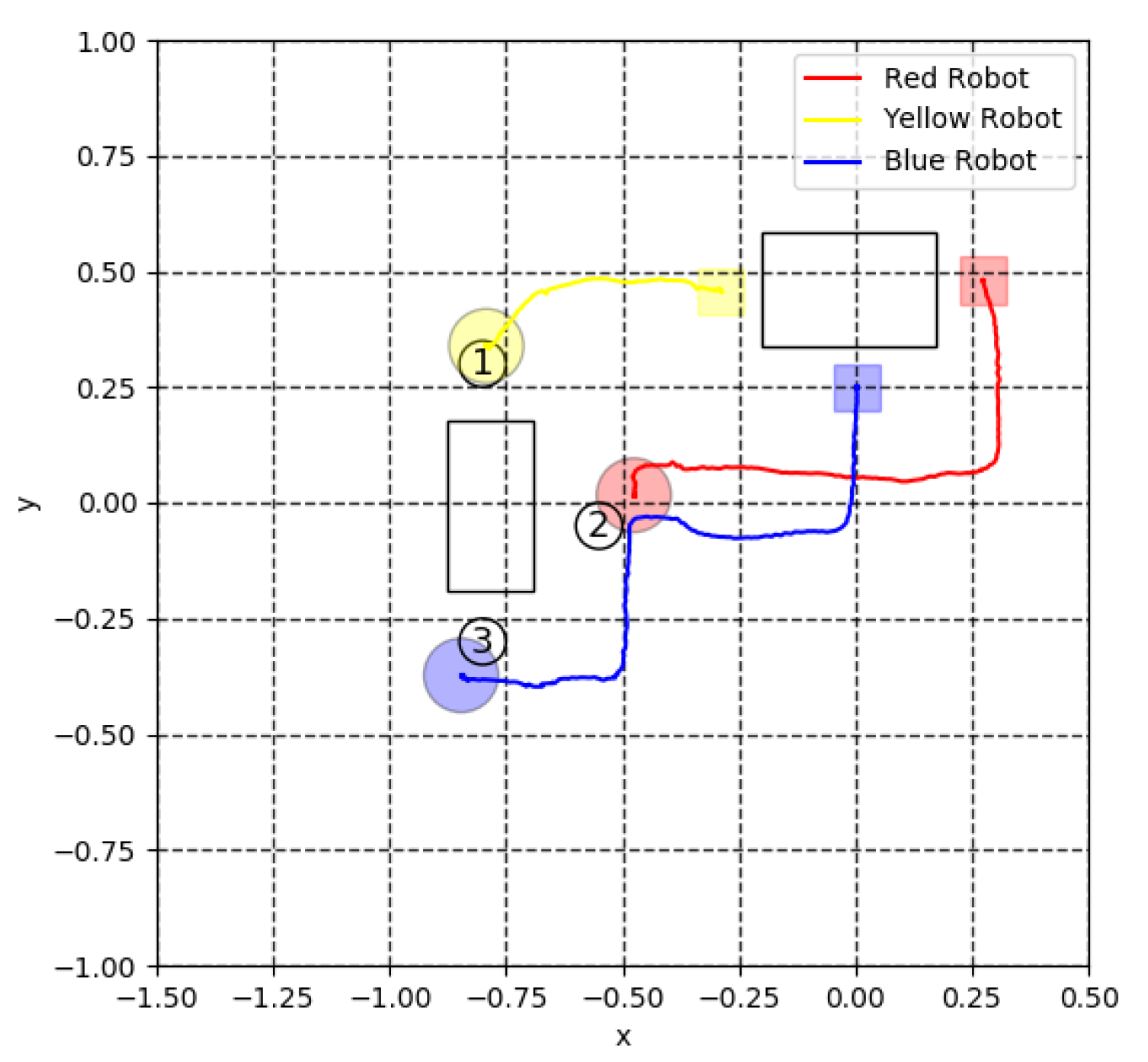
5.3. Virtual Lidar and Actual Experiment

In the actual experiment, the virtual lidar sensors were used to measure the distances between the robots and transport objects. Visualisation of the virtual lidar sensors from the ceiling camera is shown by Figure 24. As can be seen in Figure 24, the virtual lidar could detect the transport objects. The virtual lidar of the red robot could detect the transport object on the upper side of the robot while the virtual lidar of the blue robot could detect the transport object on the lower side of the robot. The virtual lidar of the yellow robot could detect the transport objects on the left side and right side of the robot.

To confirm the communication between the PC and the robots, the camera processing, and the motor controller, the velocities from the simulation were directly given to the robots. The actual experiment was implemented using the Deep Dyna-Q algorithm and the controller used was a model error compensator (MEC). In order to evaluate the performance of the MEC application in the experiment, an experiment without the MEC application was also conducted.

Figure 25 indicates the trajectory comparison of the simulation and actual experiment with the MEC, and Figure 26 shows the trajectory comparison of the simulation and actual experiment without the MEC. The velocity of each robot was derived based on the simulation result. The velocity from the simulation was implemented in the actual experiment using the MEC and without the MEC. In the actual experiment without the MEC, a PID controller was used. The values of the PID controller were set to the initial recommendation values from the robot factory. The PID values were 0.26, 0.02, and 0 for the proportional, integral, and differential values, respectively.

Comparing Figure 25 and Figure 26, the error between the simulation and the actual experiment with the MEC was smaller than without the MEC. In Figure 25, the robot path basically follows the trajectory shape of the simulation. All three of the robots have a similar trajectory to the simulation. While in the trajectory without the MEC in Figure 26, one robot follows the path of the simulation, while the other robots have a more significant gap to the simulation paths. By comparing the results of Figure 25 and Figure 26, it could be concluded that the MEC could reduce the error in the robot movement so that it has a more stable path.

Based on the results in Figure 25, the performances of the communication between the PC and the robots, the camera processing, and the MEC controller were confirmed. The next actual experiment used the random learning of Deep Dyna-Q. According to the discount rate and learning rate tuning, the best performance was chosen and applied in the actual experiment. The discount rate and learning rate used in the actual experiment were 0.9 and 0.01.

Figure 27, Figure 28 and Figure 29 show the comparison between the simulation, actual experiment with the MEC, and actual experiment without the MEC. As can be seen, all of the results in the simulation, actual experiment with the MEC, and without the MEC, could reach the target points. In Figure 28, the MEC trajectory and simulation were the same. The yellow robot (top robot) reaches target point 1, the red robot (right robot) reaches target point 2, and the blue robot (bottom robot) reaches target point 3. On the other hand, in Figure 29, even if the robots could reach the targets, there were huge errors between the actual experiment without the MEC and the simulation experiments, especially for the yellow robot (top robot) and red robot (right robot).

In summary, the simulation could predict the path by which the robots reached the target points. The MEC could control the system well in the actual experiment, which was closer to the simulated experiment path. While in an experiment without the MEC, all of the robots could achieve the target points but with a bigger error compared to the trajectory of the actual experiment with the MEC.

For testing the performance of a neural network, different layouts were presented. Figure 30 and Figure 31 show the actual experiment with the MEC on layout 1 and layout 2. The robots’ initial points are marked by the rectangle markers, while the target points are marked by the circle markers numbered 1–3. All of the robots could reach the target points properly. As shown in Figure 30 and Figure 31, all of the robots also reached the target points as well. Even in the different layouts, all robots could coordinate and achieve the target points to make the new formation in these layouts.

Figure 32 presents the cooperative transportation in an actual experiment. The formation change takes a time of about 24 s. The trajectory of this experiment can be seen in Figure 31. According to Figure 32a, the 0th second shows the initial position of the robots. Then, the movements of the robots are shown in Figure 32b,c for the 8th and 16th seconds. Finally, the robot reaches the final position at the 24th second.

The neural network learned with various random layouts, positions, and obstacle sizes to achieve the new formation form. The response in the actual experiments to the obstacles and other robots’ positions was strict in shape. In future research, the simulation and actual experiment should be reconstructed to make a digital twin system with the intention of achieving a closer result between the simulation and the actual experiment.

6. Conclusions

This study has successfully implemented the proposed method and investigated the formation control in a simulation and actual experiments. The discount rate and learning rate values affected the formation change achievement rate, collision number among agents, and collision between agents and the transport objects. For a learning rate comparison, DDQ (0.01) consistently outperformed DQN. DQN obtained the maximum −170 reward in about 130,000 episodes, while DDQ (0.01) could achieve this value in 58,000 episodes and achieve a maximum −160 reward. The application of an MEC (model error compensator) in the actual experiment successfully reduced the error in the movement of the robots so that the robots could produce the formation change appropriately.

References

1. Kamel, M.A.; Yu, X.; Zhang, Y. Formation Control and Coordination of Multiple Unmanned Ground Vehicles in Normal and Faulty Situations: A Review. Annu. Rev. Control 2020, 49, 128–144. [Google Scholar] [CrossRef]
2. Liu, X.; Liu, L.; Bai, X.; Yang, Y.; Wu, H.; Zhang, S. A Low-Cost Solution for Leader-Follower Formation Control of Multi-UAV System Based on Pixhawk. J. Phys. Conf. Ser. 2021, 1754, 012081. [Google Scholar] [CrossRef]
3. Chen, X.; Huang, F.; Zhang, Y.; Chen, Z.; Liu, S.; Nie, Y.; Tang, J.; Zhu, S. A Novel Virtual-Structure Formation Control Design for Mobile Robots with Obstacle Avoidance. Appl. Sci. 2020, 10, 5807. [Google Scholar] [CrossRef]
4. Lee, G.; Chwa, D. Decentralized Behavior-Based Formation Control of Multiple Robots Considering Obstacle Avoidance. Intell. Serv. Robot. 2018, 11, 127–138. [Google Scholar] [CrossRef]
5. Trindade, P.; Cunha, R.; Batista, P. Distributed Formation Control of Double-Integrator Vehicles with Disturbance Rejection. IFAC-PapersOnLine 2020, 53, 3118–3123. [Google Scholar] [CrossRef]
6. Liang, D.; Liu, Z.; Bhamara, R. Collaborative Multi-Robot Formation Control and Global Path Optimization. Appl. Sci. 2022, 12, 7046. [Google Scholar] [CrossRef]
7. Najm, A.A.; Ibraheem, I.K.; Azar, A.T.; Humaidi, A.J. Genetic Optimization-Based Consensus Control of Multi-Agent 6-Dof Uav System. Sensors 2020, 20, 3576. [Google Scholar] [CrossRef] [PubMed]
8. Jorge, D.R.; Daniel, R.-R.; Jesus, H.-B.; Marco, P.-C.; Alma, Y.A. Formation Control of Mobile Robots Based on Pin Control of Complex Networks. Automation 2022, 10, 898. [Google Scholar]
9. Flores-Resendiz, J.F.; Avilés, D.; Aranda-Bricaire, E. Formation Control for Second-Order Multi-Agent Systems with Collision Avoidance. Machines 2023, 11, 208. [Google Scholar] [CrossRef]
10. Ohnishi, S.; Uchibe, E.; Yamaguchi, Y.; Nakanishi, K.; Yasui, Y.; Ishii, S. Constrained Deep Q-Learning Gradually Approaching Ordinary Q-Learning. Front. Neurorobot. 2019, 13, 103. [Google Scholar] [CrossRef] [PubMed] [Green Version]
11. Ikemoto, J.; Ushio, T. Continuous Deep Q-Learning with a Simulator for Stabilization of Uncertain Discrete-Time Systems. Nonlinear Theory Appl. 2021, 12, 738–757. [Google Scholar] [CrossRef]
12. Chen, X.; Ulmer, M.W.; Thomas, B.W. Deep Q-Learning for Same-Day Delivery with Vehicles and Drones. Eur. J. Oper. Res. 2022, 298, 939–952. [Google Scholar] [CrossRef]
13. Hester, T.; Deepmind, G.; Pietquin, O.; Lanctot, M.; Schaul, T.; Horgan, D.; Quan, J.; Sendonaris, A.; Dulac-Arnold, G.; Agapiou, J.; et al. Deep Q-Learning from Demonstrations. In Proceedings of the AAAI Conference on Artificial Intelligence, New Orleans, LA, USA, 2–7 February 2018; pp. 3223–3230. [Google Scholar] [CrossRef]
14. Zhao, Y.; Wang, Z.; Yin, K.; Zhang, R.; Huang, Z.; Wang, P. Dynamic Reward-Based Dueling Deep Dyna-Q: Robust Policy Learning in Noisy Environments. In Proceedings of the 34th AAAI Conference on Artificial Intelligence (AAAI 2020), New York, NY, USA, 7–12 February 2020; pp. 9676–9684. [Google Scholar] [CrossRef]
15. Miyazaki, K.; Matsunaga, N.; Murata, K. Formation Path Learning for Cooperative Transportation of Multiple Robots Using MADDPG. In Proceedings of the International Conference on Control, Automation and Systems, Jeju, Republic of Korea, 12–15 October 2021. [Google Scholar]
16. Pitis, S. Rethinking the Discount Factor in Reinforcement Learning: A Decision Theoretic Approach. In Proceedings of the Thirty-Third AAAI Conference on Artificial Intelligence and Thirty-First Innovative Applications of Artificial Intelligence Conference and Ninth AAAI Symposium on Educational Advances In Artificial Intelligence, Honolulu, HI, USA, 27 January–1 February 2019. [Google Scholar]
17. Fedus, W.; Gelada, C.; Bengio, Y.; Bellemare, M.G.; Larochelle, H. Hyperbolic Discounting and Learning over Multiple Horizons. arXiv 2019, arXiv:1902.06865. [Google Scholar]
18. Amit, R.; Meir, R.; Ciosek, K. Discount Factor as a Regularizer in Reinforcement Learning. In Proceedings of the International Conference on Machine Learning, Online, 13–18 July 2020; pp. 269–278. [Google Scholar] [CrossRef]
19. Christian, A.B.; Lin, C.-Y.; Tseng, Y.-C.; Van, L.-D.; Hu, W.-H.; Yu, C.-H. Accuracy-Time Efficient Hyperparameter Optimization Using Actor-Critic-based Reinforcement Learning and Early Stopping in OpenAI Gym Environment. In Proceedings of the 2022 IEEE International Conference on Internet of Things and Intelligence Systems (IoTaIS), Bali, Indonesia, 24–26 November 2022; pp. 230–234. [Google Scholar]
20. Lowe, R.; Wu, Y.; Tamar, A.; Harb, J.; Abbeel, P.; Mordatch, I. Multi-Agent Actor-Critic for Mixed Cooperative-Competitive Environments. Adv. Neural Inf. Process. Syst. 2017, 30, 6380–6391. [Google Scholar]
21. Jaensch, F.; Klingel, L.; Verl, A. Virtual Commissioning Simulation as OpenAI Gym—A Reinforcement Learning Environment for Control Systems. In Proceedings of the 2022 5th International Conference on Artificial Intelligence for Industries (AI4I), Laguna Hills, CA, USA, 19–21 September 2022; pp. 64–67. [Google Scholar]
22. Budiyanto, A.; Azetsu, K.; Miyazaki, K.; Matsunaga, N. On Fast Learning of Cooperative Transport by Multi-Robots Using DeepDyna-Q. In Proceedings of the SICE Annual Conference, Kumamoto, Japan, 6–9 September 2022. [Google Scholar]
23. Sutton, R.S.; Barto, A.G. Reinforcement Learning: An Introduction, 2nd ed.; MIT Press: London, UK, 2018. [Google Scholar]
24. Bergstra, G.; Bengio, Y. Random search for hyper-parameter optimization. J. Mach. Learn. Res. 2012, 13, 281–305. [Google Scholar]
25. Peng, B.; Li, X.; Gao, J.; Liu, J.; Wong, K.-F. Deep Dyna-Q: Integrating Planning for Task-Completion Dialogue Policy Learning. In Proceedings of the 56th Annual Meeting of the Association for Computational Linguistics (Long Papers), Melbourne, Australia, 15–20 July 2018; pp. 2182–2192. [Google Scholar]
26. Su, S.-Y.; Li, X.; Gao, J.; Liu, J.; Chen, Y.-N. Discriminative Deep Dyna-Q: Robust Planning for Dialogue Policy Learning. In Proceedings of the 2018 Conference on Empirical Methods in Natural Language Processing, Brussels, Belgium, 31 October–4 November 2018. [Google Scholar]
27. Almasri, E.; Uyguroğlu, M.K. Modeling and Trajectory Planning Optimization for the Symmetrical Multiwheeled Omnidirectional Mobile Robot. Symmetry 2021, 13, 1033. [Google Scholar] [CrossRef]
28. Yoshida, R.; Tanigawa, Y.; Okajima, H.; Matsunaga, N. A design method of model error compensator for systems with polytopic-type uncertainty and disturbances. SICE J. Control Meas. Syst. Integr. 2021, 14, 119–127. [Google Scholar] [CrossRef]
Figure 1. Initial formation: The arrows represent the length and width of the cooperative transportation area, which is 4 m × 3 m.
Automation 04 00013 g001
Figure 2. Formation change.
Automation 04 00013 g002
Figure 3. Robot design.
Automation 04 00013 g003
Figure 4. Grasping using two suction cups.
Automation 04 00013 g004
Figure 5. OpenAI Gym random layout 1: The initial positions of the robots represent the start positions of the robots, shown by the yellow, red, and blue circles, while the target positions are the target set points shown by the black circles.
Automation 04 00013 g005
Figure 6. OpenAI Gym random layout 2: The initial positions of the robots represent the start positions of the robots, shown by the yellow, red, and blue circles, while the target positions are the target set points shown by the black circles.
Automation 04 00013 g006
Figure 7. Construction of Deep Dyna-Q.
Automation 04 00013 g007
Figure 8. Design of Q-network neural network.
Automation 04 00013 g008
Figure 9. Relative positions of target points (G1–3(x,y)) and other robots (R1–2(x,y)).
Automation 04 00013 g009
Figure 10. Virtual lidar (L1–16).
Automation 04 00013 g010
Figure 11. Design of transition probabilities neural network.
Automation 04 00013 g011
Figure 12. Design of reward neural network.
Automation 04 00013 g012
Figure 13. Transition reward comparison of DQN and Deep Dyna-Q.
Automation 04 00013 g013
Figure 14. Trajectories of Deep Dyna-Q with discount rate of 0.85: The robots’ initial points are marked by the rectangle markers, while the target points are marked by the circle markers numbered 1–3.
Automation 04 00013 g014
Figure 15. Trajectories of Deep Dyna-Q with discount rate of 0.9: The robots’ initial points are marked by the rectangle markers, while the target points are marked by the circle markers numbered 1–3.
Automation 04 00013 g015
Figure 16. Trajectories of Deep Dyna-Q with discount rate of 0.95: The robots’ initial points are marked by the rectangle markers, while the target points are marked by the circle markers numbered 1–3.
Automation 04 00013 g016
Figure 17. Trajectories of Deep Dyna-Q with learning rate of 0.001: The robots’ initial points are marked by the rectangle markers, while the target points are marked by the circle markers numbered 1–3.
Automation 04 00013 g017
Figure 18. Trajectories of Deep Dyna-Q with learning rate of 0.01: The robots’ initial points are marked by the rectangle markers, while the target points are marked by the circle markers numbered 1–3.
Automation 04 00013 g018
Figure 19. Trajectories of Deep Dyna-Q with learning rate of 0.04: The robots’ initial points are marked by the rectangle markers, while the target points are marked by the circle markers numbered 1–3.
Automation 04 00013 g019
Figure 20. Trajectories of Deep Dyna-Q with learning rate of 0.08: The robots’ initial points are marked by the rectangle markers, while the target points are marked by the circle markers numbered 1–3.
Automation 04 00013 g020
Figure 21. Body coordinate system.
Automation 04 00013 g021
Figure 22. Block diagram of actual implemented system.
Automation 04 00013 g022
Figure 23. Block diagram of control system.
Automation 04 00013 g023
Figure 24. Visualisation of virtual lidar sensors from ceiling camera.
Automation 04 00013 g024
Figure 25. Trajectories of simulation and actual experiment with the MEC.
Automation 04 00013 g025
Figure 26. Trajectories of simulation and actual experiment without the MEC.
Automation 04 00013 g026
Figure 27. Trajectories of simulation experiment: The robots’ initial points are marked by the rectangle markers, while the target points are marked by the circle markers numbered 1–3.
Automation 04 00013 g027
Figure 28. Trajectories of actual experiment with the MEC: The robots’ initial points are marked by the rectangle markers, while the target points are marked by the circle markers numbered 1–3.
Automation 04 00013 g028
Figure 29. Trajectories of actual experiment without the MEC: The robots’ initial points are marked by the rectangle markers, while the target points are marked by the circle markers numbered 1–3.
Automation 04 00013 g029
Figure 30. Trajectories of actual experiment with the MEC on layout 1: The robots’ initial points are marked by the rectangle markers, while the target points are marked by the circle markers numbered 1–3.
Automation 04 00013 g030
Figure 31. Trajectories of actual experiment with the MEC on layout 2: The robots’ initial points are marked by the rectangle markers, while the target points are marked by the circle markers numbered 1–3.
Automation 04 00013 g031
Figure 32. The cooperative transportation actual experiment.
Automation 04 00013 g032