Reinforcement Learning for Collaborative Robots Pick-and-Place Applications: A Case Study ^†

Abstract

The number of applications in which industrial robots share their working environment with people is increasing. Robots appropriate for such applications are equipped with safety systems according to ISO/TS 15066:2016 and are often referred to as collaborative robots (cobots). Due to the nature of human-robot collaboration, the working environment of cobots is subjected to unforeseeable modifications caused by people. Vision systems are often used to increase the adaptability of cobots, but they usually require knowledge of the objects to be manipulated. The application of machine learning techniques can increase the flexibility by enabling the control system of a cobot to continuously learn and adapt to unexpected changes in the working environment. In this paper we address this issue by investigating the use of Reinforcement Learning (RL) to control a cobot to perform pick-and-place tasks. We present the implementation of a control system that can adapt to changes in position and enables a cobot to grasp objects which were not part of the training. Our proposed system uses deep Q-learning to process color and depth images and generates an $ϵ$-greedy policy to define robot actions. The Q-values are estimated using Convolution Neural Networks (CNNs) based on pre-trained models for feature extraction. To reduce training time, we implement a simulation environment to first train the RL agent, then we apply the resulting system on a real cobot. System performance is compared when using the pre-trained CNN models ResNext, DenseNet, MobileNet, and MNASNet. Simulation and experimental results validate the proposed approach and show that our system reaches a grasping success rate of 89.9% when manipulating a never-seen object operating with the pre-trained CNN model MobileNet.

1. Introduction

Robots have been applied in industry at an increasing rate for decades [1], especially in repetitive tasks. The type of robot manipulators that are most common in industry (popularly referred to as “industrial robots”) are the so-called serial robots. They consist of links connected in series via independently actuated joints, with one or more end-effector (tool) placed at the end of the structure. The purpose of the end-effector is to act on the environment, for example by manipulating objects in the scene. The most common end-effector for grasping is the simple parallel gripper, consisting of two-jaw design.

Recently, industrial robots are being deployed in applications in which they share (part of) their working environment with people. Those type of robots are equipped with safety systems according to ISO/TS 15066:2016 [2] and are often referred to as collaborative robots (cobots). Demand for cobots is increasing also because they are easy to install, demand less space and fewer modifications in the production environment when compared to conventional industrial manipulators. Although cobots are easy to setup and program, if there is a change in the position of the objects that the robot needs to manipulate, which is expected when humans also interact with the scene, their control system needs to be adjusted. This issue is avoided if the robot is able to adjust the control system configuration in order to interact with objects in variable positions, which increases flexibility and facilitates the implementation of collaborative robotics in industrial automation.

There are many solutions to increase the above-mentioned flexibility, one of which is the application of vision systems. A few examples of computer vision applications are on food inspection [3,4], smartphone parts inspection [5], and obtaining grasping position of objects [6]. In this case, a vision technique is used to define candidate points in the object and then triangulate one point where the object can be grasped. Computer Vision has been used in industrial automation for decades [7]. More recently, the use of depth images is becoming more popular also due to the broad availability of RGBD cameras, which are sensors that acquire color images (RGB) associated with depth information (D). Several commercial models of RGBD cameras are available, like Asus Xtion, Stereolabs ZED, Intel RealSense and the well-known Microsoft Kinect, to mention a few. Depth cameras have been used in robotics to increase the amount of information a robot can get from the environment, further improving its flexibility.

Regarding the processing of visual information, several ML techniques have been applied. Deep Convolutional Neural Networks (DCNN) have been used to identify grasp positions in [8] using RGBD images as input and providing a five-dimensional grasp representation, with position $(x,y)$, a grasp rectangle $(h,w)$ and orientation ($\theta$) of the grasp rectangle with respect to the horizontal axis. Two DCNNs Residual Neural Networks (ResNets) with 50 layers each are used to analyse the image and generate the features to be used on a shallow Convolutional Neural Network (CNN) to estimate the grasp position. The networks are trained against a large dataset of known objects and their grasp position. A Generative Grasping Convolutional Neural Network (GG-CNN) is proposed in [9] as a solution to process depth images at real-time (50Hz). It uses DCNN with just 10 to 20 layers to analyse the images and depth information to control the robot in real time to grasp objects, even when they change position on the scene. Another approach to grasping different types of objects using RGBD cameras is to create 3D templates of the objects and a database of possible grasping positions. The authors in [10] used a dual Machine Learning (ML) approach, one to identify familiar objects with spin-image, and the second to recognize an appropriate grasping pose. They also used interactive object labelling and kinesthetic grasp teaching. In [11] visual control of robot manipulators is presented using Neural Network Reinforcement Learning, where specific features in the image were used to guide the robot arm control.

In this paper we investigate the use of Reinforcement Learning (RL) to control a cobot to perform pick-and-place tasks, estimating the grasping position without previous knowledge of the objects. In our previous work [12] we have presented a simulation environment to train the agent’s control system. In this paper we extend our previous work by implementing the proposed system in a real robot. We compare the performance of our RL algorithm when working with any of four pre-trained CNN models: ResNext, MobileNet, MNASNet and DenseNet. The investigation of which of the CNN models leads to the best performance in in the control of a real cobot is the main contribution of the present paper.

The remainder of this paper is organized as follows: Section 2 presents an overview of relevant concepts used in our system, such as Reinforcement Learning and Convolutional Neural Networks. The problem statement and the proposed system are described in Section 3, where the simulation and experimental setups are detailed. Section 4 describes the methodology used for training and testing the system, and Section 5 shows the corresponding obtained results. A discussion of the results is presented in Section 6 and conclusions are given in Section 7.

2. Background and Related Work

In this section we summarize relevant concepts used in the development of our system.

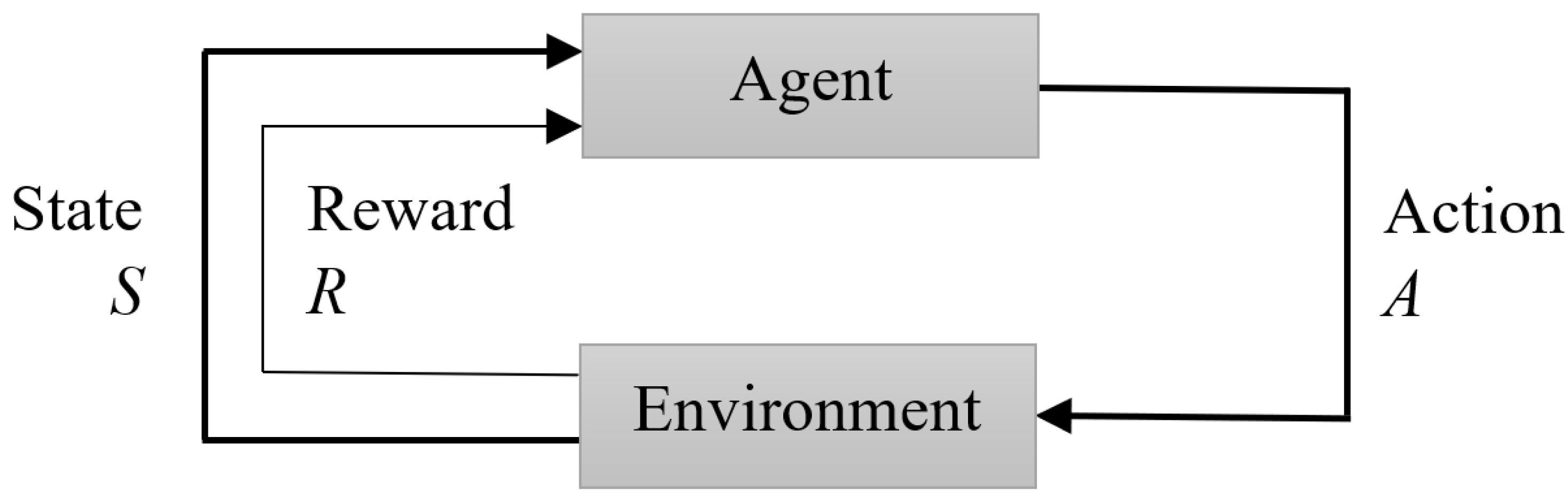
2.1. Reinforcement Learning

Reinforcement Learning is one of the three ML paradigms, along with Supervised Learning and Unsupervised Learning. In RL, the learning process occurs in the interaction of the agent with the environment via reward signals. The basic setup includes the agent being trained, the environment, the possible actions the agent can take and the reward the agent receives [13]. The reward can be associated with the action taken or with the new state. Figure 1 illustrates the principle of RL, in which an agent interacts with the environment through an action A, causes its state S to change (or not), and receives a reward R that depends on the action and state.

The control problem is often modeled as a Markov Decision Process (MDP)

$$\mathcal{M}=\{\mathcal{S},\mathcal{A},\mathcal{R},\mathcal{T},\rho ,\gamma \},$$

(1)

where $\mathcal{S}\in {\mathbb{R}}^n$ is the set of states the system can have, $\mathcal{A}\in {\mathbb{R}}^m$ are the possible actions in a given state, $\mathcal{R}:\mathcal{S}\times \mathcal{A}\mapsto \mathbb{R}$ is the scalar reward of a given action in a specific state, $\mathcal{T}:\mathcal{S}\times \mathcal{A}\mapsto \mathcal{S}$ is the transition of the system from one state to the next given an action, $\rho$ and $\gamma$ are the probability distribution of the initial states and the discount factor, respectively. The discount factor $\gamma \in [0,1)$ is used to decrease the importance of an action taken in the past [13].

The agent decides which action to take based on a policy $\pi \left(a\right|s)$ that relates the expected reward to possible actions. The policy defines what the agent should do in any situation (state). The simplest one is the greedy policy, where the agent always pursues the maximum reward. In general, greedy policies can be bad because the agent does not have motivation to explore different solutions that might lead to higher overall reward. To deal with this limitation, a common approach is to impute an exploration factor $\epsilon \in [0,1)$ as a small probability to take a random action, instead of always acting greedily.

A classical RL algorithm involves estimating the value function $V_{\pi }\left(s\right)$, which is an estimate of the value of being in a particular state. The computation of possible rewards in each state generates the value function under a policy $\pi$. The so called action-value function $Q_{\pi }\left(a\right|s)$ for a policy $\pi$ is an estimate of the value of taking action a on a given state s.

There are several methods to estimate the value function that can also be applied to the action-value function $Q_{\pi }\left(a\right|s)$. One of such methods is called Q-learning, and is defined by

$$\mathcal{Q}({\mathcal{S}}_t,{\mathcal{A}}_t)\leftarrow \mathcal{Q}({\mathcal{S}}_t,{\mathcal{A}}_t)+\alpha [{\mathcal{R}}_{t+1}+\gamma \underset{a}{max}\mathcal{Q}({\mathcal{S}}_{t+1},a)-\mathcal{Q}({\mathcal{S}}_t,{\mathcal{A}}_t)].$$

(2)

The classical Q-learning implementation creates a so-called Q-table with a combination of all actions and states. This table is usually initialized with random numbers that are updated at every interaction with the environment. It is possible to use this method with small to medium Finite Markov Decision Processes, but for large problems the size of the Q-table makes it impractical. In such cases, the Q-table needs to be approximated using other methods, such as Artificial Neural Networks (ANN), CNN and other ML algorithms.

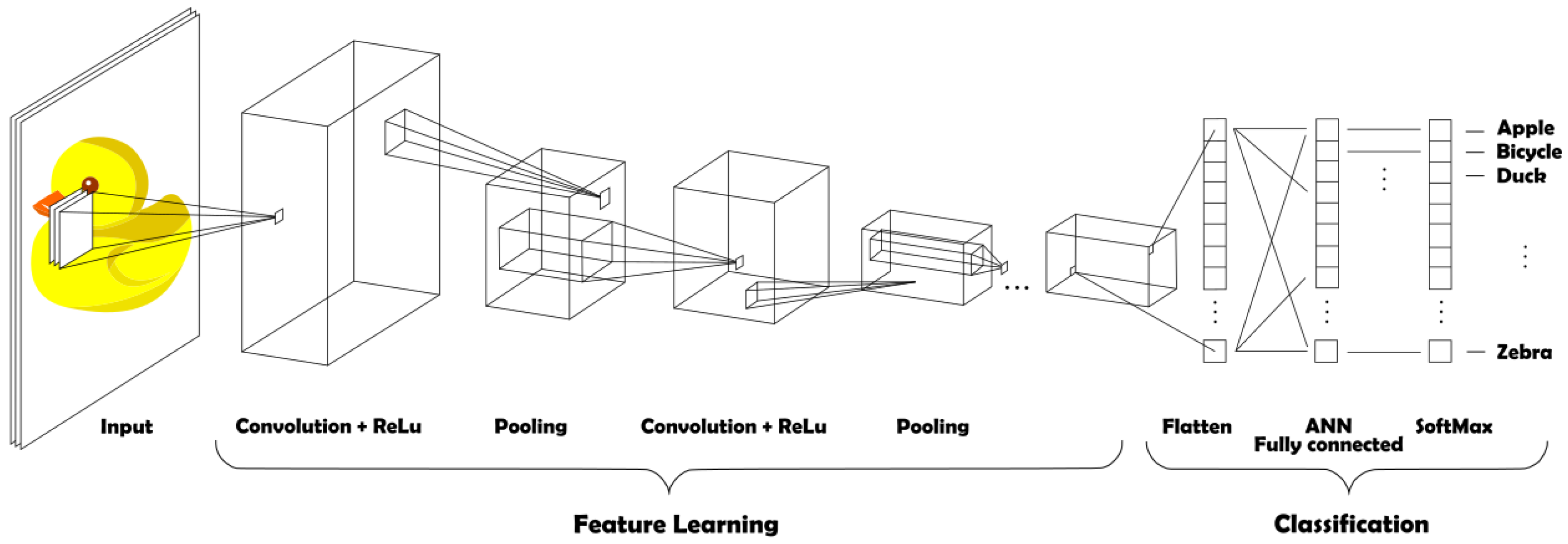
2.2. Convolutional Neural Network

CNN is a class of algorithms that use Artificial Neural Networks in combination with convolutional kernels to extract information from a dataset. The first convolutional kernel scans the feature space and stores the result in an array to be used in the next step of the CNN [14]. Figure 2 illustrates this process for an image classification problem. In the first part of the process (left), several feature arrays are extracted from the image and form the base for the next layer of convolution. After each convolution layer, pooling is performed to reduce the dimensions of the array. Then, the classification part (right) applies a fully connected ANN to output the class using an activation function. In the case of Figure 2, the softmax function normalizes the output to a probability distribution over all possible classes.

During the learning process of a CNN, the values of the kernels of the multiple convolution steps need to be determined. Such learning process can be extremely long, but once the model weights are determined, they can be stored and used in different applications.

CNNs have been applied to solve different problems in machine learning, such as object detection, natural language processing, anomaly detection, among others. Most of the CNN applications are in the field of computer vision, with a highlight to object detection and classification algorithms. In [15] a Region-Based Convolutional Neural Network (RCNN) is proposed to solve the problem of object detection. The principle is to propose around 2000 areas on the image which potentially contain an object and analyze them with a CNN in order to classify the objects in the image. One of the issues with RCNNs is the high processing power needed to perform this task. Using this technique, a modern laptop is able to analyze a high definition image in about 40 seconds, which makes it is impractical for real time video analysis.

An alternative to RCNNs is called Fast RCNN [16], in which the features are extracted before the region proposition is done, making it capable of near real time video analysis in a modern laptop. For real time applications a variation of this algorithm called Faster RCNN was proposed in [17]. It uses a technique to reduce the number of proposed objects, resulting in an algorithm capable of video analysis with an average of over 70% correct identifications. Extending Faster RCNN, the Mask R-CNN [18,19] creates a pixel segmentation around the object, giving more information about its orientation. For picking applications in robotics, Mask R-CNN also gives a hint to where to pick the detected object.

For real time applications one of the best algorithms is called YOLO, in which processing time is favored over accuracy. In its third version, YOLOv3 has an average accuracy of 50% [20] and is capable of analyzing 30 frames per second, which makes it suitable for most video processing applications [21].

Transfer Learning allows the application of previously learned knowledge to solve new problems faster or better [22]. It is popular in computer vision applications because it allows the use of a previously trained model to recognize certain patterns to solve a new problem, thus significantly reducing the necessary training time and examples. Many pre-trained models used in transfer learning are CNNs that were trained on large datasets [23]. By removing the classification part of a pre-trained CNN (see Figure 2), the remaining part that learned the feature extraction can be reused in different classification problems.

A comparison of performance between several CNN models is presented in [24]. The authors point out that a model might have different accuracy on different platforms, and there is no one-size-fits-all solution. According to them, the popular CNNs ResNet and DenseNet are heavy-weight networks, while MobileNet and MNASNet are an order of magnitude lighter in terms of required computation and memory. It is interesting to note that those four CNN models achieved similar accuracy (between 72% and 76%) when tested on ImageNet dataset on mobile devices [24]. Therefore, determining which CNN model leads to best performance on specific applications is crucial. Because of that, we are going to compare the performance of our system relative to four pre-trained CNN models: ResNext [25] (which is a variation of ResNet), DenseNet [26], MobileNet [27], and MNASNet [28].

2.3. Deep Reinforcement Learning

In RL, some problems can require more memory than is available in the system. For example, a Q-table to store all possible solutions for an input color image of 250 × 250 pixels would require $250\times 250\times 255\times 255\times 255=1,036,335,937,500$ bytes, or 1 TB of memory. For such large problems, the complete solution can be prohibitive due to the required memory and processing time, and an approximate solution can be beneficial. The use of deep learning to tackle this problem in combination with RL is called Deep Reinforcement Learning (DRL), to which the solution for playing Atari games is a classical example of successful application [29]. In approximate solutions, the Q-table can be estimated using NN, resulting in a system referred to as Deep Q-Network (DQN). DQN was proposed by [30] to play Atari games on a high level, and later this technique was also used in robotics [31]. A self balanced robot was controlled using DQN in a simulated environment with performance better than LQR and Fuzzy controllers [32]. Several DQNs for ultrasound-guided robotic navigation are presented in [33]. Finally, ref. [34] applies DRL for robotic grasping applications using RGBD images. The reported pick success rate varies from 65% to 91%, depending on the object, with higher success rates when the system uses a multi-view camera setup.

3. Problem Statement and Proposed System

In this work we address the problem of collaboration between humans and robots. We focus on the need of robots to perceive and adapt to changes in the environment while working on collaborative tasks with humans. Humans lack the precision of robots, therefore they are not likely to place objects always in the same exact position. If a cobot needs to pick up objects placed by humans, it needs to be able to deal with the variability of object positioning.

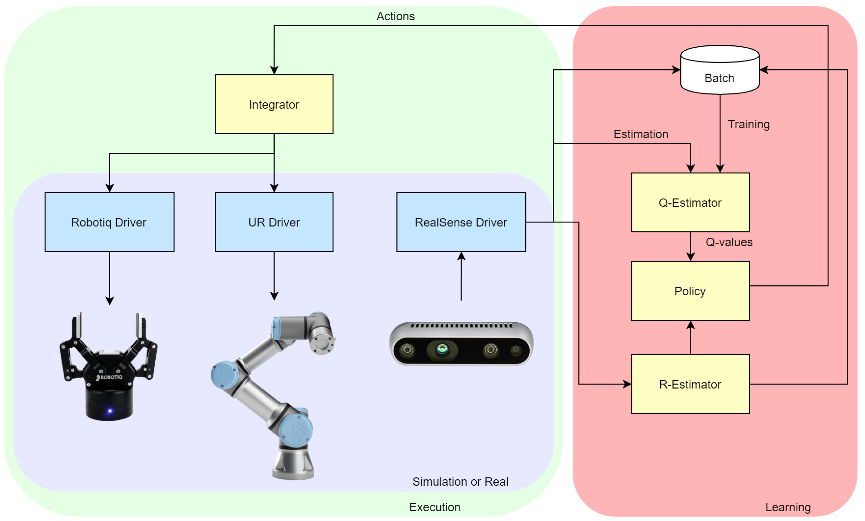
3.1. Proposed System

To address the problem described above, we propose a learning system based on Deep Reinforcement Learning to adapt to changes in object position. Unlike Supervised Learning, RL focuses on goal-directed learning from interactions and does not need labels to train the agent. Instead, it uses reward signals: each action taken by the agent is rewarded positively or negatively. For instance, in a task in which the goal is to pick certain objects from varying locations, a cobot can learn the task by trying different actions and adapting its actions based on the received rewards. After repeating the task several times, and being properly rewarded, the RL algorithm will learn how to grasp the object without the need of labeled examples. In other words, the robot trains itself to learn the grasping positions.

To enable the RL agent to execute the task, we use an RGBD camera to generate the input for a pre-trained CNN model responsible for extracting features from the images. In our previous work [12] we have shown a simulation environment to train the agent. In this paper we expand our previous work to present the implementation of our proposed system in a real robot, in which the knowledge acquired in simulation is used. We then compare the performance of our RL algorithm when working with four pre-trained CNN models: ResNext, MobileNet, MNASNet and DenseNet.

The proposed system consists of a UR3e collaborative robot equipped with a two-finger gripper and a fixed RGBD camera positioned in front of the robot pointing to the working area. A top-view of the setup is depicted in Figure 3, which shows the experimental setup (Figure 3a) and the corresponding simulation setup (Figure 3b). In both cases, the cobot is at the top of the image, and the camera is at the bottom.

The system architecture, shown in Figure 4, is divided into a Learning side (right) and an Execution side (left). In the learning side, it uses DQN to estimate the Q-values in the Q-Estimator. Actions to be taken by the robot are defined by the RL Policy. The action space is defined as coordinates for the gripper and the Q-values correspond to estimate probability of grasp success. The acquisition of experience can be accelerated in simulation, so the execution side was designed to work with both simulated environment and real hardware, for data collection, learning, fine tuning and evaluation. Robot Operating System (ROS) topics and services are used to transmit data between the learning side and the execution side. In the execution side, the boxes shown in blue are the ROS drivers, necessary to bring the functionalities of the hardware to the ROS environment. Each software module can have multiple nodes and communicate with multiple topics and services. The modules Q-Estimator, R-estimator, Policy and Integrator were written in Python as ROS modules to access the camera and the cobot. The Q-estimator module was developed using PyTorch [35] to build the DCNN to estimate the Q-values. The architecture of the DCNN was designed based on similar object detection solutions, such as in [17,18,19,21]. The Integrator converts the policy output into commands for the cobot. It identifies if the environment being controlled is real hardware or simulation and makes the proper adjustments. The Integrator is responsible for connecting all modules, simulated or real. It controls the simulation using the Supervisor API and feeds the RGBD images to the neural network. All modules were developed in Python and are available on GitHub [36] as a ROS package.

The chosen policy for the RL algorithm is a $\epsilon$-greedy, i.e., pursue the maximum reward with $\epsilon$ probability to take a random action. The R-Estimator estimates the reward based on grasping success and the actual distance to the objects reached by the gripper when performing the grasp. It is calculated as

$${\mathcal{R}}_t=\{\begin{array}{cc}\frac{1}{d_t+1},\hfill & \mathrm{if}0\le d_t\le 0.02\\ 0,\hfill & \mathrm{otherwise}\end{array},$$

(3)

where $d_t$ is the reached distance in meters.

Considering the application of RL to robotics, the necessary amount of trials and computational effort during training can grow exponentially with the number of states [37]. Abstractions can be used to reduce such high dimensionality, creating simplified representations of the state space and transferring part of the computation to a lower level controller. We adopted such approach by defining actions as coordinates to attempt to grasp an object inside the working area. The resulting action space ${\mathcal{S}}_a$ is given by

$${\mathcal{S}}_a=\{v,w\},$$

(4)

where v is the proportional position inside the working area in the x axis and w is the proportional position inside the working area in the y axis. Those values are discretized by the output of the CNN and are used as parameters for the robot moving instructions.

The architecture used to estimate the Q-values is composed by three CNNs shown in Figure 5. In the left side, the Figure shows the two pre-trained CNN models used to extract features from the images: the top one receives the RGB image as input, while the bottom one receives the depth image. The outputs of both networks are concatenated (center of the image) and fed to a third CNN that generates the final output (right side of the image). We will refer to this third CNN as output CNN because it is the one responsible for generating the Q-values.

Figure 5 shows the pre-trained CNN models as DenseNet for illustration purposes. In this work we used four pre-trained CNN models to compare their performance: DenseNet, MobileNet, ResNext and MNASNet. For each case, both pre-trained CNN models in Figure 5 were replaced by the new pre-trained CNN, while the rest of the system remained the same. The goal was to compare their computational performances in order to select the most efficient one for our case. The use of pre-trained models reduces the overall training time. However, it brings limitations to the system: the size of the input image must be 224 by 224 pixels and the image must be normalized following the original dataset mean and standard deviation [38]. In general, this limits the working area of the algorithm to an approximately square area.

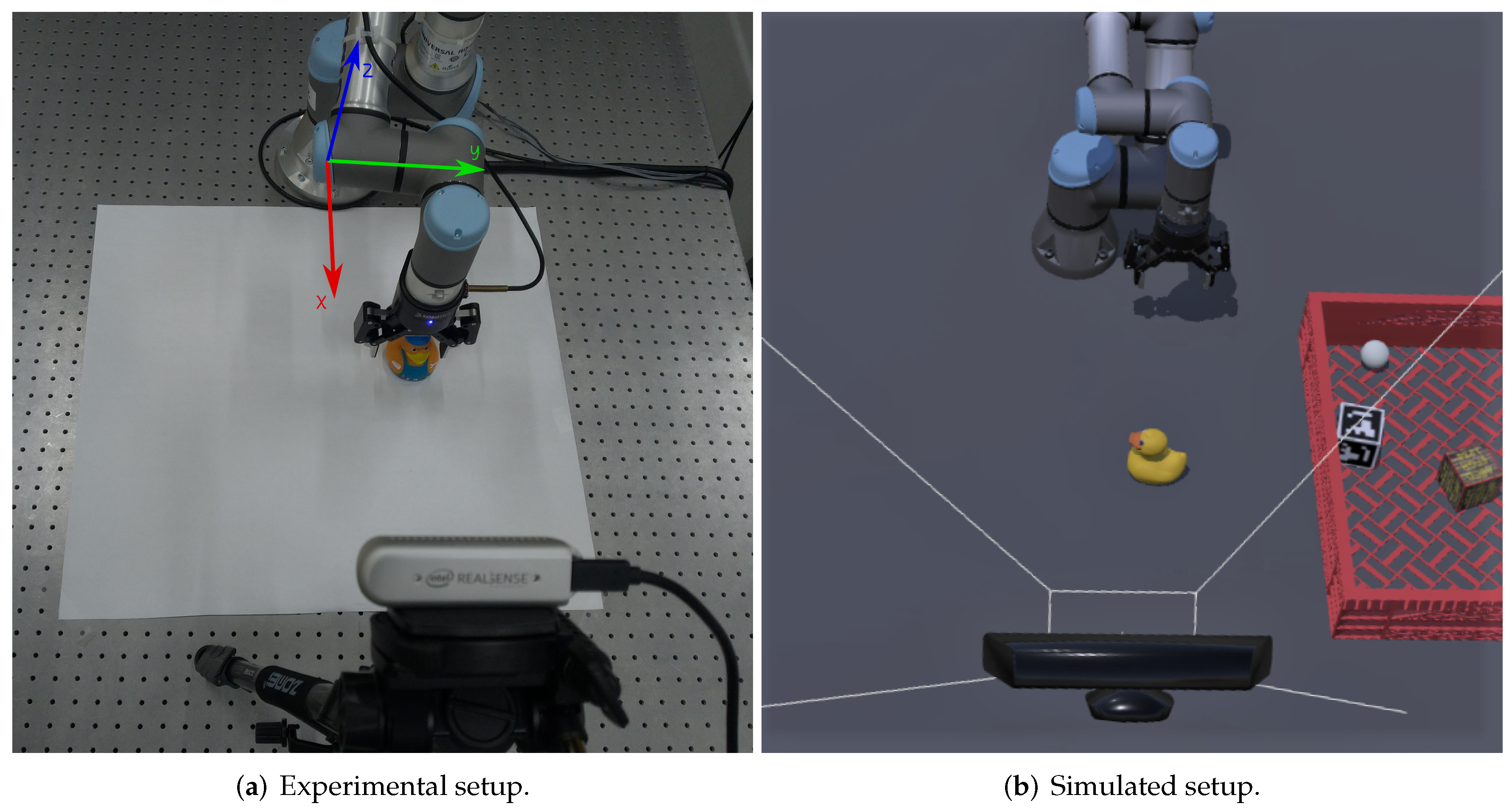
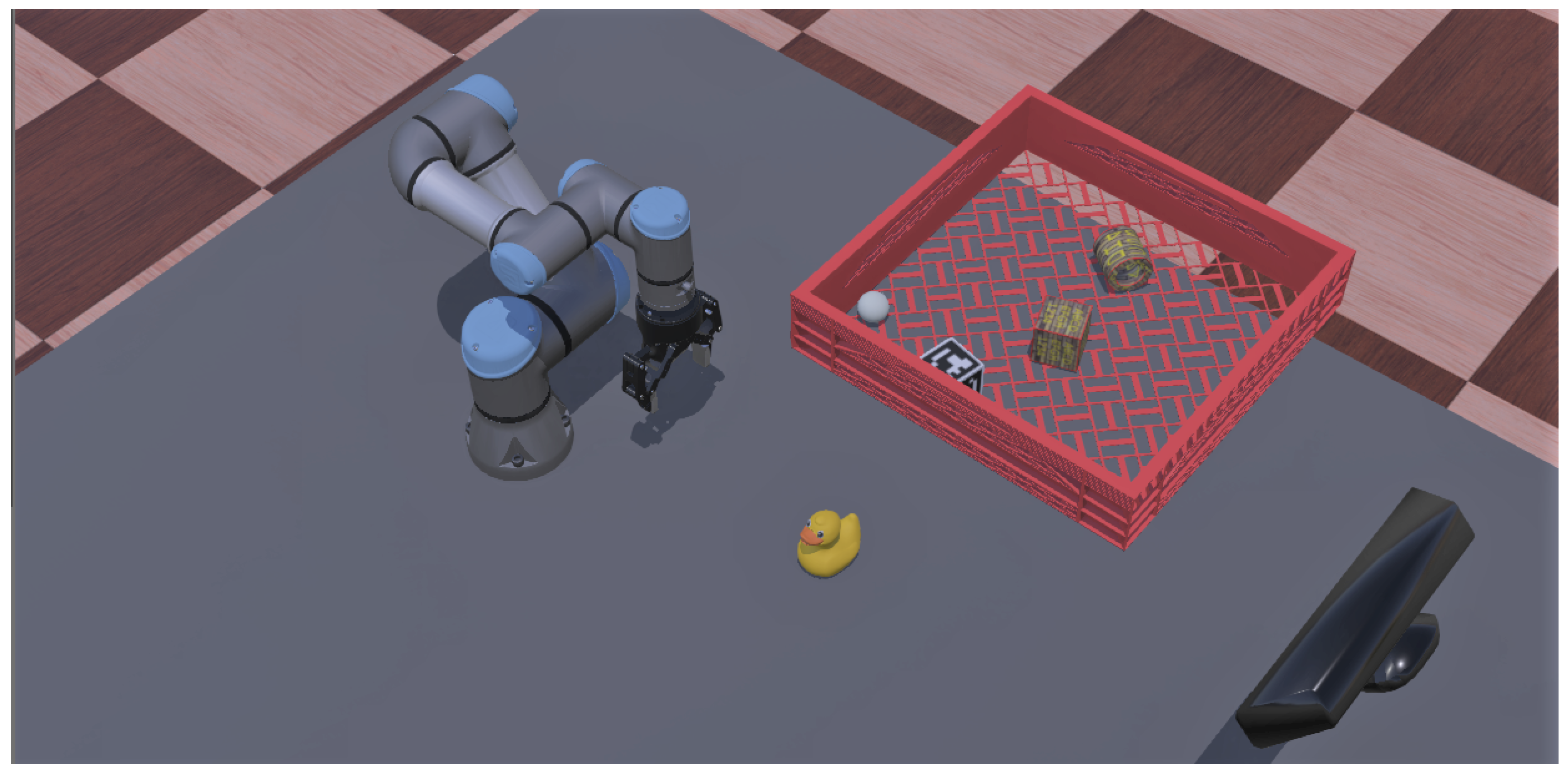
3.2. Simulation Setup

The simulation environment was built on Webots [39] because it is open-source, and due to its lower demand for computational resources when compared to similar software, like Gazebo and V-REP/CoppeliaSim [40]. To connect the simulation environment to ROS some modules were implemented: Gripper Control, Camera Control and a Supervisor to control the simulation. The simulated UR3e robot is controlled via the ROS driver provided by the manufacturer using the Kinematics module. Figure 6 shows the the simulation environment, in which the camera is located in front of the robot, pointing to the working area.

The camera used in the simulation has the same resolution and field of view like the Intel RealSense D435i camera used in the experiments. To avoid the need of calibration of the depth camera, both RGB and depth cameras were set to have coincident position and field of view in the simulation.

In the simulation we used a two-finger gripper with similar dimensions but simpler mechanical structure than the 2F-85, which was the gripper used in the experiments. The real gripper provides a signal that indicates a successful grasp. To emulate such signal, touch sensors were added at the tip of the simulated fingers to create a feedback signal that indicates when an object is grasped in the simulation. The gripper controller is responsible for controlling the position of all joints, and for reading the sensors of the simulated gripper.

The simulations were performed on a laptop with Intel Core i7-9785H CPU @ 2.6 GHz, 32 GB RAM and Nvidia GeForce GTX 1650 (Max-Q) 4 GB GDDR6, running Ubuntu 18.04. MobileNet and MNASNet were capable of running on the GPU, but DenseNet and ResNext demanded more memory than the available GPU memory from our system. Therefore, in order to compare execution time, training and timing tests were performed using only the CPU for all CNNs. Although the GPU was not used in the CNN training, the Webots simulation environment used it.

3.3. Experimental Setup

The hardware used to evaluate the performance of the proposed system consists of a Universal Robots UR3e cobot, a Robotiq 2F-85 gripper, and an Intel RealSense™ D435i RGBD camera. The software runs in ROS version Melodic Morenia [41]. Communication with the UR3e cobot was implemented using the Universal Robots ROS Driver [42], which was designed to operate with the above mentioned version of ROS. This driver allows the control of the robot via ROS while all safety features of the robot remain in operation. Interfacing with the Robotiq gripper was accomplished using drivers provided by the ROS Industrial project [43]. The interface with the RGBD camera was done with a ROS driver provided by Intel [44].

Although RL has been used to solve the kinematics in other works [34,45], this is not the case in our system. Instead, we make use of a analytical solution of the forward and inverse kinematics of the UR3e [46]. Denavit–Hartenberg parameters are used to calculate forward and inverse kinematics of the robot [47]. Considering that the UR3e has 6 joints, the combination of 3 of these can give $2^3=8$ different configurations which can give the same pose of the end-effector (elbow up and down, wrist up and down, shoulder forward and back). On top of that, the movement of the UR3e joints have a range of $(-2\pi ,+2\pi )rad$, increasing the possible solution space to $2^6=64$ different configurations for a single end-effector pose. To reduce the complexity of the problem, all joint ranges were limited in software to $(-\pi ,+\pi )rad$, still resulting in 8 possible solutions from which the nearest solution to the current position is selected. The kinematics module is capable of moving the robot to any position in the work space, avoiding unreachable positions. To increase the usability of the module, functions with equivalent behavior of the original Universal Robots MoveL and MoveJ commands [48] were implemented.

The origin of the tool reference frame (also called Tool Center Point - TCP) must be considered by the model to calculate the angles of the cobot joints to position the end-effector. The TCP is the position of the end-effector with respect to the robot flange [48]. The robot used in the experiments has a Robotiq wrist camera besides the 2F-85 gripper, which means that the gripper TCP is 175.5 mm from the robot flange in the z axis [49].

For the experiments, the architecture depicted in Figure 4 was implemented in a laptop with Intel Core i7-9785H CPU @ 2.6GHz, 32 GB RAM and Nvidia GeForce GTX 1650 (Max-Q) 4GB GDDR6.

4. Methodology

The simulation setup described in Section 3.2 was implemented and two training sessions were executed. For each training session, one of the four pre-trained CNN models was used for feature extraction: DenseNet, ResNext, MobileNet or MNASNet. Each training session is composed of several episodes. One episode is defined as one grasping attempt, divided into four steps: collecting data, deciding the action to be taken based on the estimated Q-values, executing the selected the action, and updating the weights of the output CNN based on the received reward. For training the output CNN, we used a Huber loss error function [50] and an Adam optimizer [51] with weight decay regularization [52]. The hyperparameters used in the RL and CNN models during the training process are shown in the

Table 1. Hyperparameters used in the RL and CNN models during training.

Hyperparameter	Symbol	Value
CNN Learning rate	${\alpha }_{CNN}$	1 × 10−3
CNN Weight decay	${\lambda }_w$	8 × 10−4
RL Learning rate	${\alpha }_{RL}$	0.7
RL Discount factor	$\gamma$	0.90
RL Initial exploration factor	${\epsilon }_0$	0.90
RL Final exploration factor	${\epsilon }_f$	5 × 10−2
RL Exploration factor decay	${\lambda }_{\epsilon }$	200

. To compare the performance of the 4 pre-trained CNN models, accuracy values were calculated every 10 episodes, based on 10 attempts to grasp an object.

Simulated environments allow the extraction of information and control of features that are difficult or not possible to be changed in real-world environments. To take advantage of this, in a simulation the color of the table was changed randomly at each episode to increase robustness during training. For each grasping attempt, the number of objects and their positions were also changed randomly. Finally, the positions of the object to be picked and gripper were used to calculate $d_t$ in Equation (3) to obtain the reward ${\mathcal{R}}_t$.

Two training sessions were executed in a simulation. In the first training session, no previous experience exists and the algorithm learns from scratch(as shown in Algorithm 1). In the second training session the exploration was biased through reward shaping, which has been shown to significantly reduce the number of required demonstrations, increase robustness and achieve fast learning rates [53]. Then, the resulting models from the second training session were tested with a real robot using the experimental setup described in Section 3.3. Two testing sessions were executed with the real robot: the first testing session used an object similar to one used in training, while an object never shown during training was used in the second testing session. Loss and grasping accuracy were computed and plotted for all training and testing sessions.

Algorithm 1 RL CNN Q-learning algorithm

1: Initialize: load pre trained models in the CNN 2: repeat 3:     Observe the world state s 4:     Estimate $\mathcal{Q}(\mathcal{S},\mathcal{A})$ from the forward method of the CNN 5:     Select an action in ${\mathcal{S}}_a$ with argmax of the estimated $\mathcal{Q}(\mathcal{S},\mathcal{A})$ 6:     Execute the action, observe the result 7:     if in simulation then 8:         Shape $\mathcal{Q}(\mathcal{S},\mathcal{A})$ with the expected best solution, following Equation (3) 9:     else 10:        Calculate reward R using Equation (3) 11:        Update $\mathcal{Q}(\mathcal{S},\mathcal{A})$ using Equation (2) 12:     end if 13:     Update the database with s and $\mathcal{Q}$ 14:     Use the database to train the CNN using backpropagation 15: until interrupted by the user

5. Results

In this section we present the results of the simulations and experiments described in Section 4.

5.1. Simulations

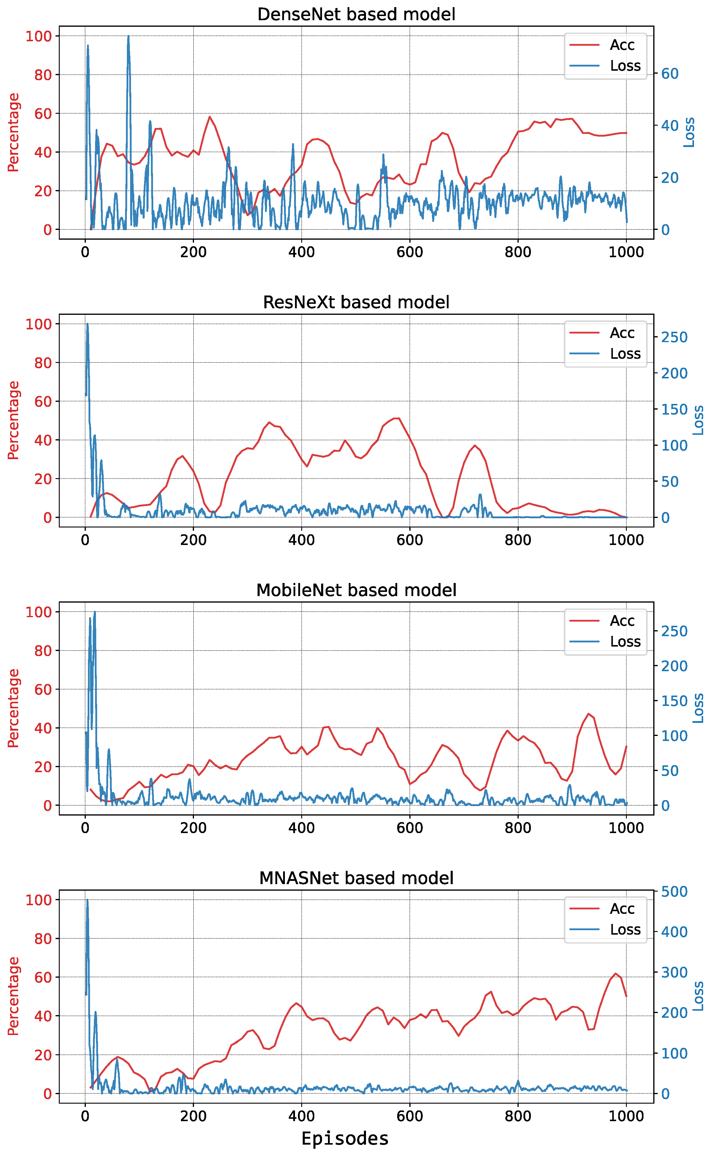
5.1.1. First Training Session

In the first training session, no previous experience existed and the algorithm learnt from scratch. The main goals were to get information about the training process on cycle time, and to acquire some experience to be used in subsequent training sessions. The forward and backward cycle times were measured for each of the four pre-trained CNN models and were presented in

Table 2. Mean time and standard deviation of forward and backward cycle times during training using the setup described in Section 3.2.

CNN Model	Forward Time [s]	Backward Time [s]
DenseNet	0.408 ± 0.113	0.676 ± 0.193
ResNext	0.366 ± 0.097	0.760 ± 0.173
MobileNet	0.141 ± 0.036	0.217 ± 0.053
MNASNet	0.156 ± 0.044	0.257 ± 0.074

. In the table, “Forward time” refers to the process following the direction from the input image to the final output CNN, while “Backward time” includes the process of evaluating the new weights of the output CNN, updated with the learning rate ${\alpha }_{CNN}$.

The forward and backward cycle times of MNASNet and MobileNet are smaller than DenseNet and ResNext. This is expected because the priors are designed to be used in smartphones and require less memory and processing power. The forward time is mostly regular and does not change much over the episodes.

To compare the performance of the 4 pre-trained CNN models, accuracy values were calculated every 10 episodes, based on 10 attempts to grasp an object. Each training session of 1000 episodes took between 1 h 43 min and 2 h 5 min to complete.

The evolution of loss and accuracy during training is shown in Figure 7 for DenseNet, ResNext, MobileNet, and MNASNet. It can be observed that for all models the loss approaches zero and remains low, while there is no sustained improvement in accuracy. This means that the algorithm cannot learn and the resulting estimated Q-values are poor.

There are several possible causes for the poor performance during the first training session, including small weights of the CNN and errors in the accumulated experience. Possible solutions for this problem can be fine-tuning of hyper-parameters, selecting best experiences [54], and using demonstration through shaping [53], for example. In demonstration through shaping, the reward function is used to generate training data based on demonstrations of the correct action to take. We applied this approach in the second training session.

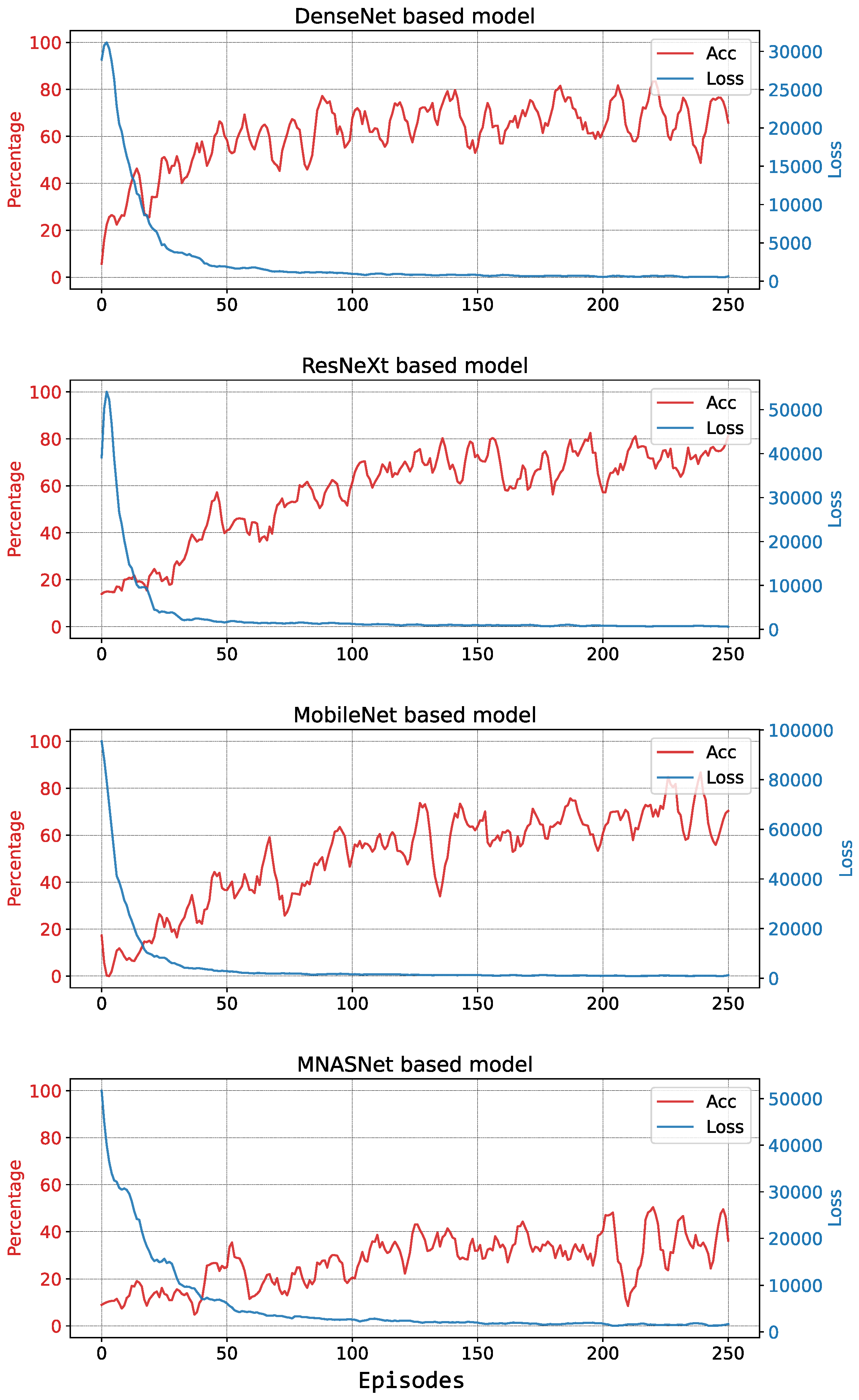
5.1.2. Second Training Session

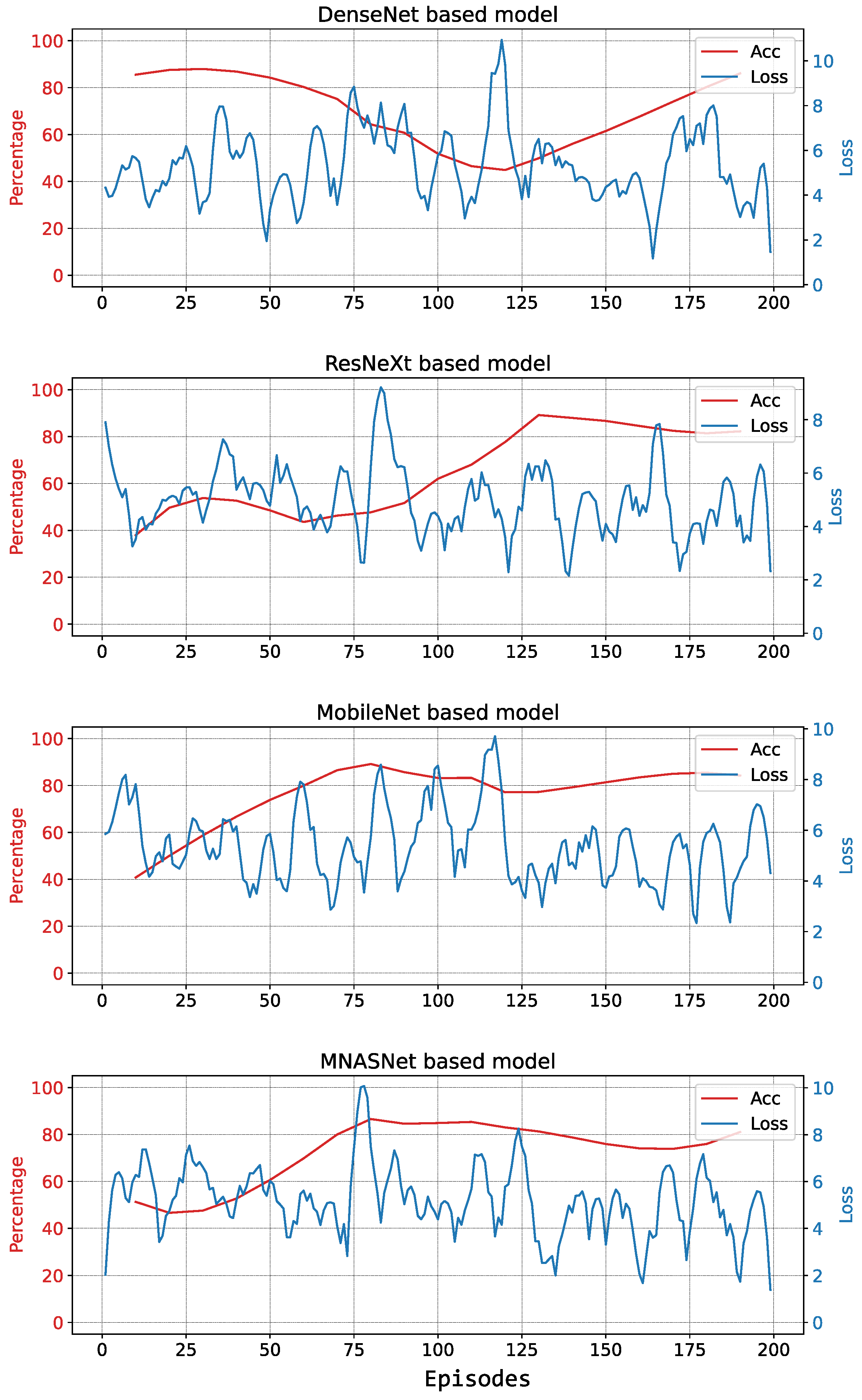
In the second training session we applied demonstration through shaping [53]. The training data for this session was generated using the reward function to map all possible rewards to the inputs. This was possible because the information of the position of the objects to be manipulated was available in simulation. The training process used knowledge about the best possible action for each episode.

The batch size used on this training session was 10. The increase of batch size, combined with the new experience replay, caused a larger loss at the beginning of the training, as seen in Figure 8. The accuracy was estimated based on 10 grasping attempts. This time, it is clear that the accuracy of the system increases with training. The second training session took much longer than the first one to complete, varying from 3 h and 43 min to 4 h and 18 min for each CNN.

5.2. Experiments

The resulting models from the second training session were tested on a real robot using the experimental setup described in Section 3.3. Two testing sessions were executed to measure the performance of the system and to verify which of the four pre-trained CNNs leads to higher accuracy with the real cobot. During both testing sessions the system continued to learn according to the description given in Section 4.

5.2.1. First Testing Session

The first testing session assesses the four models using an object similar to the one used in the training sessions: a rubber duck. Figure 9 shows the evolution of loss and accuracy for this testing session. The average accuracy achieved by the system using DenseNet, ResNext, MobileNet, and MNASNet models was 70%, 64.7%, 76.3% and 72.6%, respectively.

5.2.2. Second Testing Session

In the second testing session, the object used for gasping was a screwdriver, which was never shown during training. Figure 10 shows the evolution of loss and accuracy during the second testing session. The average accuracy achieved by the system using DenseNet, ResNext, MobileNet, and MNASNet models was 72.7%, 67.7%, 89.9% and 39.4%, respectively.

6. Discussion

Training was done in a simulation environment and the acquired knowledge was tested in a real cobot. The proposed system worked well with a real cobot, reaching maximum accuracy with the MobileNet CNN in both testing sessions (76.3% and 89.9% accuracy in the first and second sessions, respectively). It is a good level of accuracy considering its limited flexibility: it does not include the rotation of the gripper and does not consider adversarial geometry. It is interesting to note that in our previous paper [12] we reported a success rate of 84% for the same system, but that result pertains to simulation, only. Therefore, the success rate obtained in the testing session with a real cobot was even higher. The increase in success rate might be explained by the fact that during both testing sessions the system keeps learning according to the description given in Section 4. In other words, the experimental system uses knowledge gained during simulation.

As a comparison, a state-of-the-art RL grasping system that includes the motor functions in the algorithm with a dual camera setup, one in the robot wrist and an overhead camera, reached a maximum of 91.1% grasping success [34]. On the other hand, the non-RL approach described in [9] resulted on a maximum of 94% accuracy for grasping static objects and 88% accuracy when the object changes position while grasping. To achieve such results, the authors used two large datasets to train a fast CNN capable of closed-loop control.

An advantage of the RL method is the ability to continue learning even after deployment. This type of algorithm is able to continuously acquire experience and adapt its behavior. But, when considering practical applications, the main disadvantage of this technique is the enormous amount of time that is necessary for training: our setup required several hours of training to reach a usable model. The application of demonstration through shaping, where data available from simulations is used to bootstrap the model, can significantly reduce the required amount of training episodes. But the amount of time required for training is still prohibitive for many practical applications. Nevertheless, the use of RL is increasing and points to a promising future of more flexible and collaborative robotics automation.

7. Conclusions

This paper presented a case-study of the use of Deep Reinforcement Learning to provide adaptability to a cobot when performing pick-and-place tasks in the context of human-robot collaboration. We presented the architecture of our proposed system and its performance both in simulation and experiments with a real cobot. Our proposed system uses deep Q-learning to process color and depth images, and generates a $ϵ$-greedy policy to define the robot actions. The Q-values are estimated using Convolution Neural Networks based on pre-trained models for feature extraction. System performance was compared when using the pre-trained CNN models ResNext, DenseNet, MNASNet and MobileNet. Besides validating the proposed approach, results show that best performance was obtained with MobileNet, reaching of 89.9% grasping accuracy for an unknown object. This is an interesting result, especially because MobileNet is an order of magnitude lighter than ResNext and DenseNet in terms of required computation and memory. The modules created in this research are available on GitHub [36] as a ROS package and are open for community contribution. The functions to connect and control the cobot can also be reused in other applications.

References

1. Siciliano, B.; Khatib, O. Springer Handbook of Robotics; Springer International Publishing: Berlin, Germany, 2016; pp. 1–2227. [Google Scholar] [CrossRef]
2. ISO/TS 15066; Robots and Robotic Devices-Collaborative Robots. Standard, International Organization for Standardization: Geneva, Switzerland, 2016.
3. Gomes, J.F.S.; Leta, F.R. Applications of computer vision techniques in the agriculture and food industry: A review. Eur. Food Res. Technol. 2012, 235, 989–1000. [Google Scholar] [CrossRef]
4. Arakeri, M.P.; Lakshmana. Computer Vision Based Fruit Grading System for Quality Evaluation of Tomato in Agriculture industry. In Procedia Computer Science; Elsevier B.V.: Hoboken, NJ, USA, 2016; Volume 79, pp. 426–433. [Google Scholar] [CrossRef] [Green Version]
5. Bhutta, M.U.M.; Aslam, S.; Yun, P.; Jiao, J.; Liu, M. Smart-Inspect: Micro Scale Localization and Classification of Smartphone Glass Defects for Industrial Automation. In Proceedings of the 2020 IEEE/RSJ International Conference on Intelligent Robots and Systems (IROS), Las Vegas, NV, USA, 24 October–24 January 2021. [Google Scholar] [CrossRef]
6. Saxena, A.; Driemeyer, J.; Kearns, J.; Ng, A.Y. Robotic grasping of novel objects. In Advances in Neural Information Processing Systems; IEEE: New York, NY, USA, 2007; pp. 1209–1216. [Google Scholar] [CrossRef] [Green Version]
7. Torras, C. Computer Vision: Theory and Industrial Applications; Springer: Berlin/Heidelberg, Germany, 1992. [Google Scholar] [CrossRef]
8. Kumra, S.; Kanan, C. Robotic grasp detection using deep convolutional neural networks. In Proceedings of the IEEE International Conference on Intelligent Robots and Systems, Vancouver, BC, Canada, 24–28 September 2017; Institute of Electrical and Electronics Engineers Inc.: Piscataway, NJ, USA, 2017; pp. 769–776. [Google Scholar] [CrossRef] [Green Version]
9. Morrison, D.; Corke, P.; Leitner, J. Learning robust, real-time, reactive robotic grasping. Int. J. Robot. Res. 2020, 39, 183–201. [Google Scholar] [CrossRef]
10. Shafii, N.; Kasaei, S.H.; Lopes, L.S. Learning to grasp familiar objects using object view recognition and template matching. In Proceedings of the IEEE International Conference on Intelligent Robots and Systems, Daejeon, Korea, 9–14 October 2016; Institute of Electrical and Electronics Engineers Inc.: Piscataway, NJ, USA, 2016; pp. 2895–2900. [Google Scholar] [CrossRef]
11. Miljković, Z.; Mitić, M.; Lazarević, M.; Babić, B. Neural network Reinforcement Learning for visual control of robot manipulators. Expert Syst. Appl. 2013, 40, 1721–1736. [Google Scholar] [CrossRef]
12. Gomes, N.M.; Martins, F.N.; Lima, J.; Wörtche, H. Deep Reinforcement Learning Applied to a Robotic Pick-and-Place Application. In Optimization, Learning Algorithms and Applications; Pereira, A.I., Fernandes, F.P., Coelho, J.P., Teixeira, J.P., Pacheco, M.F., Alves, P., Lopes, R.P., Eds.; Springer International Publishing: Cham, Switzerland, 2021; pp. 251–265. [Google Scholar] [CrossRef]
13. Sutton, R.S.; Barto, A.G. Reinforcement Learning: An Introduction, 2nd ed.; The MIT Press: Cambridge, MA, USA, 2018; p. 552. [Google Scholar]
14. Saha, S. A Comprehensive Guide to Convolutional Neural Networks-Towards Data Science. 2018. Available online: https://towardsdatascience.com/a-comprehensive-guide-to-convolutional-neural-networks-the-eli5-way-3bd2b1164a53 (accessed on 20 June 2020).
15. Girshick, R.; Donahue, J.; Darrell, T.; Malik, J. Rich feature hierarchies for accurate object detection and semantic segmentation. In Proceedings of the IEEE Computer Society Conference on Computer Vision and Pattern Recognition, Washington, DC, USA, 23–28 June 2014; pp. 580–587. [Google Scholar] [CrossRef] [Green Version]
16. Girshick, R. Fast R-CNN. In Proceedings of the IEEE International Conference on Computer Vision, Santiago, Chile, 7–13 December 2015; pp. 1440–1448. [Google Scholar] [CrossRef]
17. Ren, S.; He, K.; Girshick, R.; Sun, J. Faster R-CNN: Towards Real-Time Object Detection with Region Proposal Networks. IEEE Trans. Pattern Anal. Mach. Intell. 2017, 39, 1137–1149. [Google Scholar] [CrossRef] [PubMed] [Green Version]
18. He, K.; Gkioxari, G.; Dollár, P.; Girshick, R. Mask R-CNN. IEEE Trans. Pattern Anal. Mach. Intell. 2020, 42, 386–397. [Google Scholar] [CrossRef] [PubMed]
19. Girshick, R.; Radosavovic, I.; Gkioxari, G.; Dollár, P.; He, K. Detectron. 2018. Available online: https://github.com/facebookresearch/detectron (accessed on 20 June 2020).
20. Redmon, J.; Farhadi, A. YOLO: Real-Time Object Detection. 2018. Available online: https://pjreddie.com/darknet/yolo (accessed on 20 June 2020).
21. Redmon, J.; Farhadi, A. YOLOv3: An Incremental Improvement. arXiv 2018, arXiv:1804.02767. [Google Scholar]
22. Pan, S.J.; Yang, Q. A survey on transfer learning. IEEE Trans. Knowl. Data Eng. 2009, 22, 1345–1359. [Google Scholar] [CrossRef]
23. Voulodimos, A.; Doulamis, N.; Doulamis, A.; Protopapadakis, E. Deep learning for computer vision: A brief review. Comput. Intell. Neurosci. 2018, 2018, 7068349. [Google Scholar] [CrossRef] [PubMed]
24. Luo, C.; He, X.; Zhan, J.; Wang, L.; Gao, W.; Dai, J. Comparison and benchmarking of ai models and frameworks on mobile devices. arXiv 2020, arXiv:2005.05085. [Google Scholar]
25. Xie, S.; Girshick, R.; Dollár, P.; Tu, Z.; He, K. Aggregated residual transformations for deep neural networks. In Proceedings of the IEEE Conference on Computer Vision and Pattern Recognition, Honolulu, HI, USA, 21–26 July 2017; pp. 1492–1500. [Google Scholar] [CrossRef] [Green Version]
26. Huang, G.; Liu, Z.; Van Der Maaten, L.; Weinberger, K.Q. Densely Connected Convolutional Networks. In Proceedings of the 2017 IEEE Conference on Computer Vision and Pattern Recognition (CVPR), Honolulu, HI, USA, 21–26 July 2017; pp. 2261–2269. [Google Scholar] [CrossRef] [Green Version]
27. Howard, A.G.; Zhu, M.; Chen, B.; Kalenichenko, D.; Wang, W.; Weyand, T.; Andreetto, M.; Adam, H. Mobilenets: Efficient convolutional neural networks for mobile vision applications. arXiv 2017, arXiv:1704.04861. [Google Scholar]
28. Tan, M.; Chen, B.; Pang, R.; Vasudevan, V.; Sandler, M.; Howard, A.; Le, Q.V. Mnasnet: Platform-aware neural architecture search for mobile. In Proceedings of the IEEE/CVF Conference on Computer Vision and Pattern Recognition, Long Beach, CA, USA, 15–20 June 2019; pp. 2815–2823. [Google Scholar] [CrossRef] [Green Version]
29. Mnih, V.; Kavukcuoglu, K.; Silver, D.; Graves, A.; Antonoglou, I.; Wierstra, D.; Riedmiller, M. Playing atari with deep reinforcement learning. arXiv 2013, arXiv:1312.5602. [Google Scholar]
30. Zanuttigh, P.; Mutto, C.D.; Minto, L.; Marin, G.; Dominio, F.; Cortelazzo, G.M. Time-of-Flight and Structured Light Depth Cameras: Technology and Applications; Springer International Publishing: Berlin, Germany, 2016; pp. 1–355. [Google Scholar] [CrossRef] [Green Version]
31. Zhang, F.; Leitner, J.; Milford, M.; Upcroft, B.; Corke, P. Towards Vision-Based Deep Reinforcement Learning for Robotic Motion Control. arXiv 2015, arXiv:1511.03791. [Google Scholar]
32. Rahman, M.M.; Rashid, S.M.H.; Hossain, M.M. Implementation of Q learning and deep Q network for controlling a self balancing robot model. Robot. Biomim. 2018, 5. [Google Scholar] [CrossRef] [PubMed] [Green Version]
33. Hase, H.; Azampour, M.F.; Tirindelli, M.; Paschali, M.; Simson, W.; Fatemizadeh, E.; Navab, N. Ultrasound-Guided Robotic Navigation with Deep Reinforcement Learning. In Proceedings of the 2020 IEEE/RSJ International Conference on Intelligent Robots and Systems (IROS), Las Vegas, NV, USA, 25 October 2020–24 January 2021. [Google Scholar]
34. Joshi, S.; Kumra, S.; Sahin, F. Robotic grasping using deep reinforcement learning. In Proceedings of the 2020 IEEE 16th International Conference on Automation Science and Engineering (CASE), Hong Kong, China, 20–21 August 2020; pp. 1461–1466. [Google Scholar] [CrossRef]
35. Paszke, A.; Gross, S.; Massa, F.; Lerer, A.; Bradbury, J.; Chanan, G.; Killeen, T.; Lin, Z.; Gimelshein, N.; Antiga, L.; et al. PyTorch: An imperative style, high-performance deep learning library. Adv. Neural Inf. Process. Syst. 2019, 32, 8026–8037. [Google Scholar]
36. Gomes, N.M. Natanaelmgomes/drl_ros: ROS Package with Webots Simulation Environment, Layer of Control and a Deep Reinforcement Learning Algorithm Using Convolutional Neural Network. Available online: https://github.com/natanaelmgomes/drl_ros (accessed on 22 January 2021).
37. Kober, J.; Bagnell, J.A.; Peters, J. Reinforcement learning in robotics: A survey. Int. J. Robot. Res. 2013, 32, 1238–1274. [Google Scholar] [CrossRef] [Green Version]
38. Models and Pre-Trained Weights. 2022. Available online: https://pytorch.org/vision/stable/models.html (accessed on 3 January 2022).
39. Webots. Commercial Mobile Robot Simulation Misc. Available online: http://www.cyberbotics.com (accessed on 18 August 2020).
40. Ayala, A.; Cruz, F.; Campos, D.; Rubio, R.; Fernandes, B.; Dazeley, R. A comparison of humanoid robot simulators: A quantitative approach. In Proceedings of the 2020 Joint IEEE 10th International Conference on Development and Learning and Epigenetic Robotics (ICDL-EpiRob), Valparaiso, Chile, 7–11 September 2020; pp. 1–6. [Google Scholar]
41. Open Robotics. Robot Operating System. Available online: http://wiki.ros.org/melodic (accessed on 18 August 2020).
42. Universal Robots. Universal_Robots_ROS_Driver. Available online: https://github.com/UniversalRobots/Universal_Robots_ROS_Driver (accessed on 5 August 2020).
43. Ros-Industrial/Robotiq: Robotiq Packages. Available online: http://wiki.ros.org/robotiq (accessed on 19 October 2020).
44. Intel(R) RealSense(TM) ROS Wrapper for D400 Series, SR300 Camera and T265 Tracking Module: IntelRealSense/realsense-ros. 2019. Available online: https://github.com/IntelRealSense/realsense-ros (accessed on 3 January 2022).
45. Rajeswaran, A.; Kumar, V.; Gupta, A.; Vezzani, G.; Schulman, J.; Todorov, E.; Levine, S. Learning Complex Dexterous Manipulation with Deep Reinforcement Learning and Demonstrations. Technical Report. arXiv 2017, arXiv:1709.10087. [Google Scholar] [CrossRef]
46. Hawkins, K.P. Analytic Inverse Kinematics for the Universal Robots UR-5/UR-10 Arms; Technical Report; Georgia Institute of Technology: Atlanta, GA, USA, 2013. [Google Scholar]
47. Universal Robots-Parameters for Calculations of Kinematics and Dynamics. Available online: https://www.universal-robots.com/articles/ur/application-installation/dh-parameters-for-calculations-of-kinematics-and-dynamics/ (accessed on 31 December 2020).
48. Universal Robots. Universal Robots e-Series User Manual-US Version 5.7. 2020. Available online: https://www.universal-robots.com/download/manuals-e-series/user/ur5e/57/user-manual-ur5e-e-series-sw-57-english-us-en-us/ (accessed on 5 August 2020).
49. Robotiq Inc. Manual Robotiq 2F-85 & 2F-140 for e-Series Universal Robots, Robotiq Inc.: Québec, QC, Canada, 7 November 2018.
50. SmoothL1Loss - PyTorch 1.7.0 Documentation. Available online: https://pytorch.org/docs/stable/generated/torch.nn.SmoothL1Loss.html (accessed on 15 January 2021).
51. Kingma, D.P.; Ba, J.L. Adam: A method for stochastic optimization. In Proceedings of the 3rd International Conference on Learning Representations, ICLR 2015-Conference Track Proceedings. International Conference on Learning Representations, ICLR, San Diego, CA, USA, 7–9 May 2015. [Google Scholar]
52. Loshchilov, I.; Hutter, F. Decoupled Weight Decay Regularization. arXiv 2017, arXiv:1711.05101. [Google Scholar]
53. Brys, T.; Harutyunyan, A.; Suay, H.B.; Chernova, S.; Taylor, M.E.; Nowé, A. Reinforcement learning from demonstration through shaping. In Proceedings of the IJCAI International Joint Conference on Artificial Intelligence, Buenos Aires, Argentina, 25–31 July 2015; pp. 3352–3358. [Google Scholar]
54. De Bruin, T.; Kober, J.; Tuyls, K.; Babuška, R. Experience selection in deep reinforcement learning for control. J. Mach. Learn. Res. 2018, 19, 1–56. [Google Scholar] [CrossRef]
Figure 1. Reinforcement Learning principle: the agent interacts with the environment through an action A, changing its state S and receiving a reward R (adapted from [13]).
Automation 03 00011 g001
Figure 2. CNN process for an image classification problem: in the Feature Learning part, several convolutional layers alternate with pooling; in the Classification step, a fully connected ANN is used to define the output of the process (adapted from [14]).
Automation 03 00011 g002
Figure 3. Experimental (a) and simulated (b) setups showing the Universal Robots UR3e cobot, its gripper, and the position of the RGBD camera. Figure (a) also shows the base reference frame of the robot, with respect of which all positions are measured.
Automation 03 00011 g003
Figure 4. Proposed architecture divided in execution (left) and learning (right) sides. The modules in blue are ROS Drivers and the modules in yellow are Python scripts.
Automation 03 00011 g004
Figure 5. The CNN architecture for the action space S a . The two main blocks are a simplified representation of pre-trained Densenet model. Only the feature size is represented. The features from the Densenet model are concatenated and used to feed the CNN that generates the Q-values used to determine the robot action.
Automation 03 00011 g005
Figure 6. The virtual environment built on Webots: it consists of a table, a UR3e cobot (left) with a two-finger gripper, an RGBD camera (right) and the objects to be manipulated by the robot.
Automation 03 00011 g006
Figure 7. Evolution of loss and accuracy during 1000 episodes of the first training session. For all models, loss remains low while there is no sustained improvement in accuracy. The blue line shows loss data smoothed using a third order filter.
Automation 03 00011 g007
Figure 8. Evolution of loss and accuracy during 250 episodes during the second training session with demonstration through shaping. The blue line shows loss data smoothed using a third order filter.
Automation 03 00011 g008
Figure 9. Evolution of loss (blue) and accuracy (red) of the system during 200 episodes of the first testing session on a real robot. Data was smoothed using a third order filter.
Automation 03 00011 g009
Figure 10. Evolution of loss (blue) and accuracy (red) of the system during 100 episodes of the second testing session on a real robot. Data was smoothed using a third order filter.
Automation 03 00011 g010