Abstract
The enhancement of new quality criteria in highway construction is a key aspect to improving the construction process and lifetime of road. In particular, mobile laser scanning systems are nowadays able to provide realistic 3D elevation profiles of a road to detect anomalies. In this context, this study utilizes a high-accuracy high-speed mobile mapping vehicle and evaluates a weighted longitudinal profile as an improved measure for evenness analysis. For comparison a classical method with a rolling straight edge was evaluated on the same road section and observed effects are discussed. The second focus is the areal reconstruction of the road thickness. For this purpose, a modern method was developed to spatially synchronize two high-speed laser scans using reference boxes next to the road, to transfer the point clouds into a surface model and to calculate the layer thickness. This procedure was conceptually validated by some pointwise measurements of the layer thickness. With this information, imperfections in the base layer could be detected automatically over a wide area at an early stage and countermeasures might be initiated before constructing the highway.
1. Introduction
Road construction and especially the enhancement of its production process is a key focus to improve transport infrastructure in many countries. Since growing traffic volume increases the strain on road networks, they need to be properly built and maintained. Concrete construction plays an important role in this aspect, as it has, if properly built, a longer service life with less maintenance requirements and is more resilient to heavy duty traffic [1,2]. In recent years, the automation of construction site machinery and processes on a construction site has evolved [3,4,5]. Furthermore, new evaluation criteria for the existing highway network as well as for new constructions are being investigated [6,7].
In this context, Torres et al. [5,8] also evaluated the general gaps in automation and provided guidelines for highway construction. They identified data acquisition and management as crucial limiting factors to automation for road construction in the US. In addition, some of the used machines and technologies do not produce or provide sufficient access to relevant data for road quality control.
An area where more complex data acquisition and computation methods have shown great promise, is surface layer scans and their use to generate 3D surface profiles and road thickness information. The surface evenness is limited by the manufacturing process. Commonly stringlines are used to guide the paver to achieve a defined road profile and even surface. The surface quality is additionally influenced by the smoother, being directly attached to the paver as well as various post processing steps such as brushing or grinding.
The surface evenness in Germany is commonly measured using contacting methods such as rolling straightedges (RSE) [9] but is more and more replaced by 1D and 2D laser scans as non-contacting measures. In addition, 3D elevation profiles are generated using 2D laser scans. Due to higher road quality requirements and an improved laser scan accuracy, 3D laser scanning techniques have been extensively researched in the past years for a variety of different applications [10,11]. The advantage of 3D elevation profiles is that they more accurately represent the three-dimensional characteristic of the road surface and are able to inspect the whole road surface instead of only one line. Mobile laser scanning systems, in particular, provide the advantage of being able to record an entire road while driving. However, a tradeoff between the measurement grid, the vehicle speed and the achieved laser scan precision arises. Commonly, a 2D laser scan is conducted at a defined recording frequency while the vehicle is driving. If the vehicle increases its speed, the distance between the grid points in the direction of travel increases likewise. In addition, since the measurement equipment is mounted on a car which is excited by various unevenness during driving, the distance of the laser scanner to the surface varies leading to errors. Thus, an inertial measurement unit (IMU) or similar measurement equipment and complex calculations are required to compensate for these errors to achieve a high accuracy.
Most mobile laser scanning systems described in the literature focus on road system mapping and road feature extraction such as those summarized in [10,11]. In these cases, the precision of the laser scanners ranges between some millimeters up to centimeters. Thus, no highly accurate road surface profiles can be extracted. On the other hand, Puente et al. [12] employed a mobile mapping system for surface scans. However, they limited the vehicle speed to 20 km/h and recorded with only a precision of the laser scan of about 8 mm. Research by De Blasiis et al. [13] employed a similar technique but was already able to conduct measurements with a vehicle speed of 55 km/h with a line scan distance of 7 cm. Still, current research focuses either on very accurate laser scans or on collecting data over a large area. Little research is available on high-speed and high-accuracy 3D laser scanning technology, which can be used to qualify a road surface.
Besides providing an accurate 3D scan of the whole surface at a high speed, a simplified measure is often desired to quantify the road surface evenness to gain an acceptance certificate for the built road. In this context, geometric methods or response type methods such as the International Roughness Index (IRI) are used [13,14]. The weighted longitudinal profile (WLP) combines advantages of geometric methods and response type methods and is currently being researched in Germany. One prerequisite for such advanced evaluation methods is that the 3D surface evenness can be recorded at a high accuracy.
Another aspect of evaluating the final road quality is road thickness. Similarly to surface evenness, road thickness is commonly predefined and maintained by using stringlines as a reference during paving. The location of the stringline is measured and calibrated at defined supporting points once before paving. This method requires intensive calibration effort and offers the highest accuracy at the defined grid points [15]. The road thickness, however, is also influenced by unevenness in the base layer, which are not covered by the stringlines.
Measurement methods for the road thickness are commonly locally limited manual or visual methods. For example, a destructive but accurate method for thickness evaluation is to draw drill cores. Alternatively, steel rounds can be placed on the base layer which can later be detected by non-destructive measurement principles. Likewise, ground penetrating scanners can be used but they might not be accurate enough [16]. Most of these manual measurement methods lead thus to a high effort if many locations needed to be evaluated. Furthermore, they do commonly not automatically collect and record the data for later use.
If 3D profiles of the road surface and base layer are easily obtainable by mobile LiDAR measurements, they might also be utilized to provide road thickness information. Some studies on this topic have been conducted in the compaction of earthen structures. For example, Meehan et al. [17] evaluated the lift thickness for earthen embarkments. They employed a RTK-GPS attached to the compactors to measure the placed soil and its compaction. The accuracy of this method was also reported in [18] to be sufficiently accurate for earthworks but might be insufficient for road thickness evaluations.
In the context of road pavements, Walters et al. [19] presented a first study to utilize laser scans of the base layer and top layer of a concrete road. However, a stationary laser scanner was used. A study by Puente et al. [12] expanded that concept by actually recording the base layer and finished road surface by using a mobile measurement vehicle with GPS/INS, LiDAR, and cameras. However, the vehicle speed was only 20 km/h, with a limited resolution of the scanner of 8 mm. The synchronization between the different test drives was achieved by using retro-reflective targets. This was extended by a study by González-Jorge et al. [20], where the accuracy of different targets for the synchronization of different mobile laser scans was evaluated. They showed that the accuracy of pavement thickness estimation lies within 2 to 3 cm for suitable sensor targets. On the other hand, Liu et al. [21] presented a real-time road elevation measurement directly before and after paving. However, the described approach utilizes a mobile platform attached to the paver which is tracked by a robotic total station instead of a mobile laser scanning system.
Thus, this research utilizes a mobile mapping vehicle, which is equipped with modern LiDAR instruments. It can be used to record highly accurate topographies of a road surface over a wide area at high travel speeds, even in moving traffic. The measurement vehicle can record both the base layer of the road before paving and also the surface of the finished road. This data can be used for two purposes: First, the surface scan of the finished road provides a 3D evenness map over the whole road instead of a locally limited 2D profile as provided by RSE or profilograph and more advanced evaluation criteria like the WLP [7,22]. This leads to an improved surface evaluation and can be used to identify and post-process areas with a large unevenness. Second, the surface scan of the base layer can be used to quantify the surface evenness before paving. In combination with the surface scan after paving, the road thickness can be calculated. In addition, it can be identified if variations in the base layer evenness result in similar variations in the final surface. The estimated road thickness can be used to draw drill cores at critical areas instead of predetermined locations, to improve critical areas before the road is released, or to add preventive measures if e.g., the surface of the base layer shows larger imperfections.
One essential prerequisite for such advanced methods is that the data are available in a common database and framework, e.g., by using common coordinates, which can be identified in all measurements. This is required since the relative accuracy of the 3D scans in terms of surface measurement is high but the absolute positioning of the measurement vehicle e.g., using GNSS is limited. The aim of this research is thus to show that 3D laser scans do not only provide a high-accuracy 3D surface profile of the whole road to reliably detect surface unevenness, but to also provide a proof of concept that this data can be used to generate an estimate of road thickness and its variation.
Thus, the main contributions of this study are
- To discuss the evenness of the road surface with classical and new methods by using real highway construction site data;
- To demonstrate the feasibility of high-speed high-accuracy multitemporal laser scan technology in combination with the Weighted Longitudinal Profile;
- And to implement and verify an areal road thickness analysis based on spatially synchronized multitemporal laser scans for a real construction site.
Background information on a construction site and the challenges are provided in Section 2. The measurement technology and analysis methods are described in Section 3. The road evenness is evaluated based on mobile LiDAR measurements. The same measurement principle is then used to estimate the areal road thickness. Section 4 discusses the results of the 3D surface profile and the derived evenness and thickness. The findings are concluded in Section 5.
2. Road Construction and Evaluation
To understand some of the challenges in concrete road construction, the road design and production process is introduced at first. The general road layout of a typical German highway is presented in Figure 1. Before a road is paved, a base layer (hydraulically bound, asphalt) is built as a basis. In this case, a two-layer pavement with an asphalt base layer is shown. A thicker bottom layer is built at first and immediately afterwards, a finer top layer is installed. Since the concrete shrinks during hardening and temperature changes, the concrete surface needs to be cut thus leading to transverse and longitudinal joints. The concrete slabs are connected via tie and dowel bars to prevent the slabs from moving. Once the road work is finished, the sides, guardrails, and signs are installed.
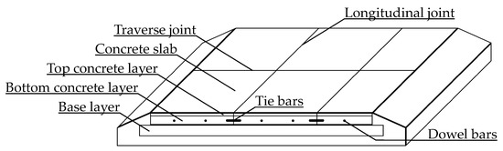
Figure 1.
General road layout [23].
The construction process itself is illustrated in Figure 2. The mixing plant produces the concrete by mixing raw materials such as cement, water and coarse, and fine aggregates. The material is loaded onto dumpers. If a two-layer road is paved, both the bottom layer and top layer concrete need to be mixed and transported to the construction site. In this case, two adjacent slipform pavers, as shown in Figure 3, install the concrete. At first, the bottom layer is paved, followed by the top layer. In the end, a retarding agent is sprayed on top of the surface to slow down the hardening. In addition, the dowel bars are either placed or vibrated into the concrete. The surface is additionally brushed and cut to achieve a proper surface grip, to reduce noise emissions, and to prevent the road from cracking. Once all downstream operations have been completed and the concrete has sufficient strength, the road can be opened to traffic. The duration of the different process steps is illustrated in Figure 2 to highlight the different time constants of the production steps. For further details refer to [23].
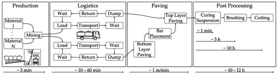
Figure 2.
Construction site participants and exemplary work flow [23].
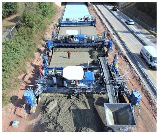
Figure 3.
Two-layer concrete paving and spraying.
The final road quality can be influenced by variations and issues within each process step. In this case, focus is laid on the evaluation of the final road and especially the surface quality. Possible influencing factors during paving can be assigned to the categories of concrete quality and especially its workability, continuity of the paving process, accuracy of the bar placement, reference tracking to achieve a consistent thickness and surface, environmental conditions and logistics, and pre-distribution of the concrete. For example, if the hardening process of the concrete is too evolved then the paver will have difficulties to provide an even surface or cavities might occur. If the concrete quality is within limits, a continuous compaction using vibrators influences the properties of the concrete road as e.g., described in [24]. A continuous speed during paving leads to a high material throughput and might improve the surface quality due to less stop and go procedures. Therefore, the logistics (mixing, transport) has to function well. Unfavorable weather conditions during paving, e.g., extremely low or high temperatures or heavy rain showers, can hinder the curing process, alter the consistency of the concrete, or even lead to defects in the surface. Delays in the delivery of concrete impair the workability of the concrete or force the paver to stop reducing productivity.
Accurate tracking of the road location, e.g., using a stringline or high-accuracy GPS, is essential to keep the exact course of the road and a steady elevation profile. Surface evenness and texture play an important role in ride comfort and safety. An uneven surface leads to vibrations or induces periodic excitations, which affect the driving experience and increase stress on the road. The surface quality is for example influenced by the paving process, irregularities during the construction process, e.g., where manual work is required or at transitions between different pavement types, and surface post processing through brushing, cutting, and sometimes also grinding.
Furthermore, constant road thickness needs to be maintained. Variations in the road thickness might result in different road properties such as load-bearing strength and reduce durability, especially if some road segments become too thin. Small variations in the road thickness occur naturally since the surface of the base layer is typically less even. However, if these variations become too large, they might either lead to reduced road thickness in some areas or to a similar large unevenness in the final road surface, if the road thickness is to be kept constant. Since these variations might occur randomly and in a small area, standard road surface and body evaluation methods might not recognize them. Thus, possible failures due to these effects are only detected after years of operation.
3. Measurement and Analysis Methodology
Two quality criteria of the finished road—the surface evenness and the road thickness—are evaluated on a highway construction site during regular operation. Examples on how the relevant data can be recorded, preprocessed, and evaluated to achieve a smart construction site as described in [23] are provided. At first, the measurement methods and equipment are introduced.
3.1. Road Evenness Evaluation Based on Mobile LiDAR Data
With increasing traffic loads, especially the rising proportion of heavy-duty traffic, higher demands are also placed on the evenness of a road surface. In particular, unevenness in the road surface significantly influences the dynamic portion of the wheel load and can thus lead to disproportionate damage to the road structure [25].
The evenness of a surface in Germany is commonly evaluated using a 4 m RSE [9]. Simplified, a 4 m long bar is supported by 10 wheels. In between, a measurement wheel is installed which can move up and down to record surface deviations. A schematic of the working principle is given in Figure 4. The RSE is pulled along the road to generate a 2D surface profile along one line. Areas of high unevenness which occur not directly along the travel path of the RSE are not detected. Thus, more advanced methods such as 2D and 3D laser scanning and wavelet analysis [22,26,27,28] are being researched.
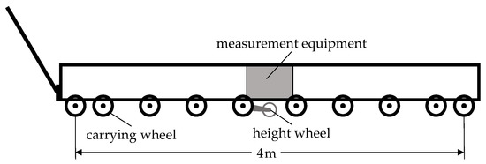
Figure 4.
Schematic of a rolling straightedge.
In Germany, non-contact methods are based on the high speed road monitoring method (HRM), in which four laser distance sensors are used in a linear arrangement for the long- and short-distance road excitations [9]. Since the classical contacting measurement methods and HRM have the drawback of mapping only limited wavelength ranges [29], more complex evaluation methods have been investigated in recent years. These address the aspects of ride comfort, safety, and surface durability more comprehensively than possible with the previous detection technologies and evaluation indicators [28,30]. In addition, modern recording methods, such as mobile laser scanning, enable a fast recording of road surfaces. Thus, 3D laser scans represent the three-dimensional characteristic of a road surface more adequately than a two-dimensional representation in the form of elevation profiles. A comparative study between classic non-contact measurement methods and the acquisition of a longitudinal profile from laser light-sectioning and laser scanning is the subject of an ongoing research project of the Federal Highway Research Institute [31]. As a result, this technology is systematically evaluated and tested for its feasibility.
In the following, the weighted longitudinal profile (WLP) [7,22], a modern evaluation approach for the analysis of longitudinal evenness is presented. This approach will be introduced into regulations and standards for German and European levels. The underlying evaluation of the WLP combines the advantages of conventional geometric methods, such as the virtual rolling straight edge or profilograph simulations, and response type methods, such as the International Roughness Index [14], which also take into account aspects of vehicle dynamics. The WLP thus ensures an objective evaluation of irregularly and periodically occurring unevenness, but also of local single events. Here, a transformation process is used to emphasize short waves with comparatively low amplitudes via a weighting function. This enables the short- and long-wave excitations contained in the true longitudinal profile of a road surface to be assessed using the same evaluation scale (millimeters). Since periodicities contained in the longitudinal profile of a road can lead to resonance phenomena of the vehicle and consequently to a noticeable loss of comfort, a special octave band filtering is applied. Thus, short irregularities occurring at regular intervals receive an appropriate weighting.
In detail, a longitudinal height profile is converted into a frequency spectrum by means of a fast Fourier transformation (FFT) and scaled to equal the power spectral density by the evaluation function . The weighted spectrum:
is divided into a total of nine octaves ranging from a wavelength of 0.2 m to 102.4 m and transformed back into spatial domain …. The WLP:
is the weighted sum of the nine octave band filtered, weighted partial height profiles. The weighting factors are chosen based on the standard deviation of the corresponding partial height profile . The parameter is the sum over all weighting factors . Further details can be found in [7,9,22]. Figure 5 visualizes the calculation scheme of the WLP . Two indicators are derived to describe the WLP. This first indicator is the standard deviation:
and the difference between maximum and minimum:
over an evaluation section. The parameter n is the number of profile points in the evaluation section. The proposed evaluation section lengths for road monitoring on a network scale are 100 m for federal highways and 20 m for urban areas. For approval after construction, an evaluation section length of 20 m is proposed [7].
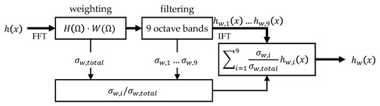
Figure 5.
Calculation scheme for the weighted longitudinal profile (WLP) [22].
Where conventional non-contact measurement methods only record individual longitudinal height profiles along the line of travel, modern LiDAR instruments can be used to record highly accurate topographies of the road surface over a wide area at high travel speeds, even in moving traffic. The kinematic multi-sensor system S.T.I.E.R of the company Lehmann+Partner [32] is a measuring system for the acquisition of longitudinal and transverse evenness, three-dimensional surface as well as surface appearance of roads and traffic areas. Figure 6 shows the mobile mapping vehicle S.T.I.E.R. The core components of S.T.I.E.R are an inertial positioning system, laser distance sensors for measuring a longitudinal height profile in the right-hand rolling lane (HRM), a surface LiDAR system, and various camera systems for recording the vehicle environment and the road surface. Optionally, the modular Mobile Mapping System can also be expanded with additional sensor technology, such as an environment laser scanner. For this study, the relevant data sources are the pavement laser scanner (LiDAR), the environment scanner (LiDAR), and the inertial positioning system.
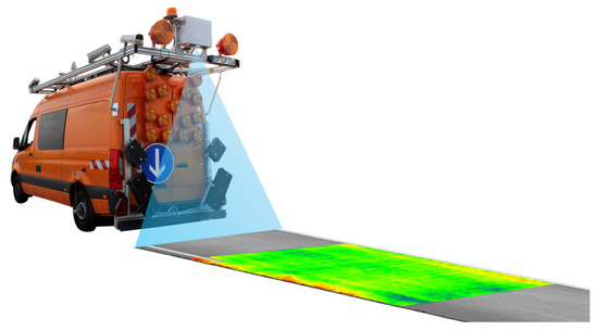
Figure 6.
S.T.I.E.R measurement vehicle and schematic representation of laser scan.
The S.T.I.E.R positioning system is an integrated system consisting of a global navigation satellite system (GNSS), an inertial measurement unit (IMU), and a distance measuring instrument (DMI). The combination of these components enables the determination of both absolute position and relative position change, including all solid angles and accelerations. The absolute accuracy of the trajectory after post-processing of the inertial positioning system data is specified as 20 mm for the x-y-position and 50 mm for the altitude [33]. The surface laser scanner is a Pavement Profile Scanner Plus (PPS) from the Fraunhofer Institute for Physical Measurement Techniques [34]. The PPS measures 1 million points per second with approx. 920 points per scanned profile. The measurement accuracy of the PPS, averaged over a 10 cm × 10 cm surface element, is in the sub-millimeter range. To ensure this extremely high precision at high measurement speeds and simultaneous eye safety, the PPS uses the phase shift technology and a wavelength in the near infrared range as the measurement principle [35].
The basic data in terms of dense 3D point clouds for further investigations is created by synchronizing the measurements of the positioning system and the laser scanner over time. On an acquisition width of approx. 4.2 m, a surface measurement is taken transversely to the direction of travel approximately every 4.5 mm. Such scan profiles are generated every 28 mm at a driving speed of 80 km/h. A 4 m × 5 m concrete slab is therefore scanned with approximately 0.2 million measuring points. Figure 7 top shows such a laser scan of a concrete pavement. A higher density of measuring points in the direction of travel can be achieved by reducing the driving speed. From these disorganized 3D point clouds, a regular measurement point grid aligned with the trajectory is generated (3D surface model), as it is also used in the automotive sector for simulation purposes [36]. For evenness analysis in the context of road condition detection and assessment, a grid size of 0.1 m in longitudinal and transverse direction is relevant [9]. Due to the ordered matrix structure of the 3D surface model, longitudinal and transverse profiles with absolute elevation values can be efficiently extracted at arbitrary locations and fed to a evenness analysis based on the WLP or other indicators. Figure 7 bottom shows the described 0.1 × 0.1 m 3D surface model superimposed with green dots on the point cloud.
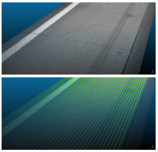
Figure 7.
Laser scan of a concrete pavement (top) and superimposed 3D surface model in a 0.1 × 0.1 m grid (bottom).
The second LiDAR instrument, which can be integrated on the measurement vehicle as required, is the Clearance Profile Scanner (CPS) also manufactured by the Fraunhofer Institute for Physical Measurement Techniques. The CPS is a rotating laser scanner for recording clearance profiles, which measures according to the phase shift technology. By rotating a mirror, the laser scanner records a 2D profile in a recording range of 350. The CPS is mounted in the rear area of the vehicle’s roof rack and it is aligned in such a way that the individual profiles are recorded transversely to the direction of travel. Due to the movement of the measuring vehicle, the laser beam describes a helix, whereby the road space is successively scanned along the trajectory in an approximately 30 m wide corridor. The CPS achieves a data rate of 1–2 MHz and records approximately 200 profiles per second with 5000–10,000 points per profile. The accuracy of the length measurement is 3 to 7 mm at a distance of 5 m, depending on the reflective properties of a surface [37].
3.2. 3D Analysis of the Concrete Paving Thickness Using Multitemporal Mobile Laser Scanning
In addition to assessing the evenness, the investigations on the test section also focused on determining the installed layer thickness of the concrete pavement, as this is a decisive factor in the standardization and calculated dimensioning with regard to the service life of a road. The determination of the layer thickness is typically carried out selectively and randomly with classical methods by comparing the planned and actual layer thickness, either by taking drill cores or non-destructively by inserting control bodies between the base and the concrete layer. Statements about spatial patterns are not possible with these methods. This requires an area analysis of both the base layer and the concrete surface.
As explained in Section 3.1, mobile LiDAR systems can be used to acquire high-resolution three-dimensional surface scans of the pavement. In an analogous procedure, a surface model of the base can be generated before the concrete pavement is installed. On the one hand, such multi-temporal measurements make it possible to check on a profile-by-profile basis whether unevenness in the base has an effect on the evenness of the manufactured surface. On the other hand, volume-based analysis or change detection analysis [38] can also be carried out. Hereby, the quality of the spatial data synchronization plays a decisive role in the derivation of absolute differences between temporally offset data recordings. In mobile mapping systems, the absolute positional accuracy of the acquired 3D data is largely determined by the GNSS conditions at the time of data acquisition. Even after integrating additional support sensors (IMU, DMI) of the inertial positioning system, the positioning solution is only accurate by a few centimeters, especially with regard to the height component. Through the additional integration of terrestrially measured control points or relative link points, which are visible in all time slices of data acquisition, the spatial synchronization of multitemporal laser scans can be decisively improved. Thus, these dense-meshed 3D data can also be used for the analysis of the manufactured thickness of the concrete pavement. Therefore, reference boxes were set up in the side space of the construction site to serve as relative linking points for multitemporal laser scans. As Figure 8 shows, these boxes are 0.45 × 0.45 × 0.45 m in size and were attached to stationary objects, such as sign structures. The CPS environmental laser scanner was used to track these boxes because the reference boxes were outside the field of view of the PPS.
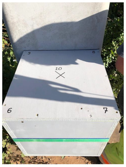
Figure 8.
Reference box used for spatial synchronisation of multitemporal laser scans.
Figure 9 shows on the left two exemplary laser scans of the CPS before and after installation of the concrete pavement. In the right, the two scans are shown spatially synchronized. The syncronisation is performed using Iterative Closest Point Registration on the visible surface planes of the reference box [39]. The reference box, which was attached to a traffic sign structure, served as the terrestrial control point for synchronization. Along the z-axis, the distance between the 3D points of the base and surface layer can be calculated and interpreted as an approximation of the paving thickness.
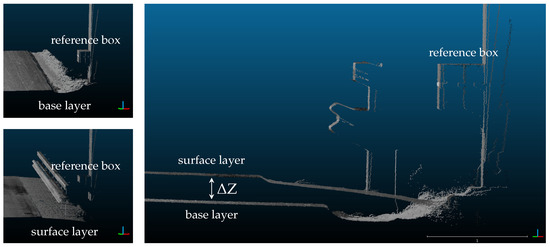
Figure 9.
Principle of difference formation of base and surface layer scan for approximation of the paving thickness Z.
The thickness estimation based on the laser scans was backed up by a few manual thickness evaluations. In this case, a non-destructive method based on steel rounds and pulse induction (PI) measurements was used. The steel rounds were placed on the surface of the base layer before paving. In addition, drill cores were used as a destructive method to gain additional information about the road properties and thickness.
4. Results
For an evaluation of the proposed methods, a typical concrete highway construction site in Germany was considered. On the site, reference boxes for spatial synchronization were installed and the base and surface layer were recorded using high-speed laser scanning and a classical RSE. The following two sections present the evenness results as well as the results for the proof of concept for areal thickness analysis.
4.1. Evenness Evaluation Results
A 7 km long section of a highway concrete construction site was recorded with a planograph and the mobile mapping vehicle S.T.I.E.R of the company Lehmann+Partner was used to analyze the longitudinal evenness. In parallel to the pure measurement records, all anomalies were documented manually during the planograph inspection. The camera system on the measuring vehicle was also used to identify irregularities. This makes it possible to explain observed effects in retrospect. As the construction period was in autumn with a lot of rain, no standard conditions prevailed for the laser scan due to the surface moisture. This may have a negative effect on the scatter in the laser scan data and slightly influence the WLP indicators.
In addition to the measured RSE, a straightedge simulation was performed based on the processed laser scan data in the right rolling lane of the first lane. Both the real and calculated profile were then shifted along the driving direction until the peaks overlapped to synchronize the two measurement series. Since the RSE uses an odometric measurement system for position determination and the two measurement series were not collected exactly on the same trajectory, these measurement series are also slightly distorted against each other. This effect can be neglected because the WLP indicators WLP and WLP are averaged over a range of 20 m and the maximum chainage deviation of the peaks between RSE and the straightedge simulation is 1 m.
In Figure 10, a 1.5 km long section of the evenness analysis is shown. A direct comparison between the values of the RSE and WLP is difficult due to the different measurement and calculation principles. Hence, differences in the evaluation trajectory between the RSE and the height profile used for the WLP calculation can show different effects. However, the same tendencies can clearly be observed. One advantage of the measurement via S.T.I.E.R is that the camera pictures are available at each location. Thus, the anomalies within the profiles can be investigated. The two vertical red marks at a chainage of 113,662 and 113,763 indicate a change in the material between concrete and asphalt. This area is shown on the left of Figure 11. Unevenness is often unavoidable at such locations. In the direct comparison of the measurement series, a good agreement between the RSE and the WLP indicators is observable. According to Ueckermann et al. [22] and Maerschalk et al. [7], the type of cause of the unevenness can be interpreted by the relationship between and . A strong excitation of is an indication of a geometric single event and a excitation of indicates a dynamic periodic unevenness in the pavement. The RSE and the WLP indicators show a deflection at the positions where the material changes as well as at a chainage of 114,775. All these effects can be attributed to an unevenness caused by a single geometric event which is clearly visible in the camera pictures. This is also supported by the observation that the dominates the . The peculiarity in the area between 114,230 and 114,300 is probably due to the fact that paving started there anew due to an overnight shift change. Figure 11 on the right shows that the appearance of the surface changes in this area. This is a sign that a long interruption during road installation occurred. The surface is typically post processed, e.g., brushed and cut, once the concrete is sufficiently hardened. Since the hardening process of the concrete is influenced by different environmental factors such as temperature and humidity, the workers have to gradually check for the right surface hardening. Thus, some areas might show a different surface appearance. Since the peculiarity is only observable in the WLP, a dynamic excitation based on more smaller, single geometric events could be present until the whole installation process has properly restarted and all process steps have returned to a steady production state. However, this assumption cannot be confirmed at the present time and further information needs to be collected. In the range from chainage 113,800 to 114,000 a small dynamic periodic unevenness in the surface might be present because the dominates the . Such unevennesses cannot be represented by the RSE measurements.
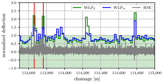
Figure 10.
Evenness analysis for the first lane. The evenness indicators rolling straightedges (RSE), WLP, and WLP are shown normalized to their respective targeted value (4 mm and 24 mm).
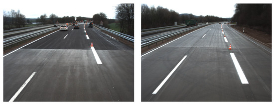
Figure 11.
Camera views of the material change (left) and at the start of the day (right).
The area highlighted in green in Figure 10 shows the range of unevenness permitted by German regulations. Besides the previously investigated peculiarities, the highway was installed within the applicable tolerances and shows good quality.
4.2. Concrete Paving Thickness Results
The 3D laser scan profiles demonstrated that an accurate surface scanning for both the base layer and the finished road is possible. As a result, the measurements can be used to provide a proof of concept of an automated road thickness evaluation. As described in Section 3.2, an experimental approach based on multitemporal laser scanning was designed and implemented for a 100 m long section of a highway construction site for the areal analysis of the pavement thickness. One of the reference boxes described above and shown in Figure 8 was used as a terrestrial control point for the spatial synchronization of the laser scans recorded at different time instances (before and after paving). While the box was still completely visible in the base layer laser scan, it was partially shadowed by the guardrail at the time of the surface layer scan. Despite the resulting limitation for the point cloud matching, a synchronization of the data sets could be achieved by means of the Iterative Closest Point Registration with an RMSE of 9 mm. The left image in Figure 12 shows the situation before synchronization. The points represent the front and top of the reference box viewed from the side. The colors white and red denote the base and surface layer scan, respectively. The GNSS-induced global shift between the two scans is clearly visible and amounts to approximately 22 mm in height. The right image shows the situation after synchronization, where all red points are transformed using the translational shifts along x-y-z of the Iterative Closest Point Registration. The deviations between the two scans are now only in the range of the measurement noise of the CPS scanner.
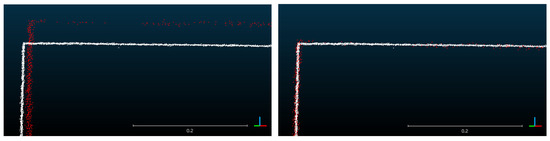
Figure 12.
Cross-section through the reference box before (left) and after (right) matching the multitemporal laser scans.
After the laser scans of the base and surface layer were spatially synchronized, the scan areas of the pavement were isolated as separate point cloud clusters from the remainder of the scan (side-strip, inventory, etc.). Subsequently, the surface clusters of base and surface layer were reduced to a 10 × 10 cm grid using inverse distance weighting. The noise of the 3D measurement points on the base and surface layer is in the range of 4 to 7 mm and 4 to 6 mm, respectively and has about halved due to the grid. Afterwards, a triangulated irregular network (TIN) surface was calculated using Delaunay triangulation. Thus, areas with lower measurement point sampling or sporadic data gaps are closed. Finally, the difference between the TIN of the surface layer and the TIN of the base layer can be interpreted as an approximation of the absolute pavement thickness.
To support and validate this laser scan-based method, steel rounds were inserted in the relevant section between the base layer and the concrete pavement, and PI measurements were carried out at these points after installation. Figure 13 illustrates the obtained 3D thickness information over the whole road area. In addition, the location of the non-destructive measurement points A and B is shown. A drill core was taken at position C. The position of the reference box is marked by a square. In the background the slab structure of the pavement and the road markings are visualized. The paving thickness is shown as relative deviation from the road thickness at point C, since the drill core position is clearly visible in the laser scan. In the georeferenced surface model, shades of blue describe thicker road thickness and yellow to red indicates a thinner road thickness. In the middle and at three quarters of the section, a slight reduction in thickness can be observed in lane 1. At the end, an increase in paving thickness can be seen. Thus, local effects in the road thickness are clearly visible.
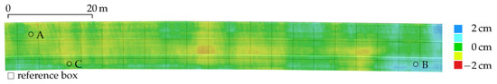
Figure 13.
Relative layer thickness and location of the test points A–C with slab structure and road markings in the background.
The comparison with point-by-point PI measurements of steel rounds and the evaluation of the drill core proves the plausibility of the values derived from the mobile laser scans. At point C, the drill core indicates a 3 mm thicker absolute layer thickness than was reconstructed with the laser scan. Points A and B have a deviation of 20 and −8 mm. However, their position cannot be located very accurately in the laser scan data. The presented approach cannot replace classical approaches for the determination of the absolute pavement thickness, but it allows the identification of local patterns or discontinuities and can give indications where imperfections in the base layer may have to be taken into account when finishing the concrete pavement. For example, areas of significantly lower thickness than the planned pavement thickness can be identified. This can be particularly useful when comparing the base layer scan to the planned surface layer to identify where imperfections in the base course could lead to a critical pavement thickness.
Figure 14 shows a vertical cut through the pavement approximately along the middle of lane 1. The detrended height profiles of the base and surface layer are drawn over the distance. Here, imperfections (small bumps) in the base layer of the pavement can be observed at 35 to 50 m and at 75 to 90 m. These imperfections do not appear in the surface layer, which shows that the paving process is able to cope with such imperfections in the base layer. On the other hand, this leads to a reduced road thickness at these locations. This effect is also amplified by a small hollow at 50 m in the surface layer. In this case, the road thickness is still within the defined limits. However, if these imperfections become too large, it might become critical to maintain the desired road thickness. Thus, the scan of the base layer helps to identify deviations in the base layer and to react to them at an early stage as well as to estimate the road thickness and to identify peculiarities, which can then be investigated in detail.
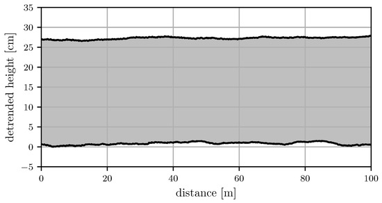
Figure 14.
Cross-section of the pavement approximately along the middle of lane 1.
5. Conclusions
The evenness and thickness of a pavement represent two central evaluation criteria for the quality and durability of construction work during road construction. These evaluation criteria are essential to identify dominant process variables, which become especially relevant in the context of the advancing digitization of construction process execution and the improvement in data acquisition and management systems.
Therefore, this study investigated a classical standardized evenness measurement method as well as new indicators of evenness based on high-speed multitemporal laser scanning. The measurements of different data collection systems were synchronized based on distinct events. In particular, specific height profiles were identified for combining the RSE and laser scan and stationary reference boxes were applied to correct the absolute absolute offset of the different measurement runs of the mobile mapping vehicle S.T.I.E.R. The 3D laser scan provided valuable surface evenness data over the whole construction site. The occurring irregularities could be identified and explained by specific effects seen both in the manual site documentation and on the basis of the camera system of the measuring vehicle. The WLP provided additional insight into some irregularities which were not observable by the standard RSE.
The second aspect of the study was the experimental determination of the capability to measure the road thickness using high-speed laser scans. For this purpose, the base and surface layer were scanned with a laser measurement vehicle. Reference boxes, which are visible in both measurements, were attached to permanent structures next to the pavement so that the laser scans can be spatially synchronized. The feasibility of the presented method could be validated by additional pointwise thickness measurements based on the pulse induction method using steel rounds and drill cores. The investigated road section showed a local imperfection in the base layer, which affects the road thickness. However, further investigations have to show the accuracy and robustness of the proposed method. Therefore, this method can currently only be used as an aid, e.g., for identifying interesting positions for further investigation. In addition to the possibility of an area-wide road thickness measurement, the presented method for road thickness determination offers the significant advantage that the planned location of the layer can already be examined for a potential reduction in pavement thickness before the start of the construction of the concrete layer. This way, preventive countermeasures can be taken at an early stage.
For further analyses, a detailed documentation of the process steps and an extensive data set of the construction machine fleet, not only for surface scan but also for concrete production, transport, paving, and post-processing, is available for this highway section. The data will be used in further studies to provide additional insight into a smart construction site.
Author Contributions
Conceptualization and methodology, P.S., M.S., S.R., A.G. and O.S.; investigation and analysis P.S., M.S., S.R., T.B.; data curation, T.B., M.S.; writing—original draft preparation, P.S., M.S. and S.R.; writing—review and editing, T.B., A.G., O.S.; supervision, project administration and funding acquisition, H.G. and O.S. All authors have read and agreed to the published version of the manuscript.
Funding
This research was funded by the Federal Highway Research Institute (BASt), Germany, 88.0151/2017 and partially supported by the Deutsche Forschungsgemeinschaft (DFG, German Research Foundation) under Germany’s Excellence Strategy—EXC 2120/1-390831618.
Institutional Review Board Statement
Not applicable.
Informed Consent Statement
Not applicable.
Data Availability Statement
Not applicable.
Acknowledgments
The authors thank Barbara Jungen of the Federal Highway Research Institute (BASt) and Steffen Scheller of LEHMANN+PARTNER GmbH for their support. In addition, the authors express their gratitude to the contributors Heinz Schnorpfeil Bau GmbH, Liebherr-Mischtechnik GmbH, Wirtgen GmbH, Otto Alte-Teigeler GmbH, LEHMANN+PARTNER GmbH, CAVEX GmbH, and the Materials Testing Institute (MPA), and the Institute of Construction Materials (IWB) of the University of Stuttgart. The authors are responsible for the content of the paper.
Conflicts of Interest
The authors declare no conflict of interest.
Abbreviations
The following abbreviations are used in this manuscript:
| RSE | Rolling Straightedge |
| WLP | Weighted Longitudinal Profile |
| LiDAR | Light Detection And Ranging |
| GNSS | Global Navigation Satellite System |
| HRM | High Speed Road Monitoring |
| FFT | Fourier Transformation |
| IFT | Inverse Fourier Transformation |
| S.T.I.E.R | Mobile Mapping Vehicle |
| IMU | Inertial Measurement Unit |
| DMI | Distance Measuring Instrument |
| PPS | Pavement Profile Scanner Plus |
| CPS | Clearance Profile Scanner |
| PI | Pulse Induction |
| RMSE | Root Mean Squared Error |
| TIN | Triangulated Irregular Network |
References
- Oesterheld, R.; Peck, M.; Villaret, S. Straßenbau Heute Band 1: Betondecken; Bau + Technik GmbH: Erkrath, Germany, 2018. [Google Scholar]
- Delatte, N.J. Concrete Pavement Design, Construction, and Performance; CRC Press: Boca Raton, FL, USA, 2014. [Google Scholar] [CrossRef]
- Kuenzel, R.; Teizer, J.; Mueller, M.; Blickle, A. SmartSite: Intelligent and autonomous environments, machinery, and processes to realize smart road construction projects. Autom. Constr. 2016, 71, 21–33. [Google Scholar] [CrossRef]
- Liu, D.; Lin, M.; Li, S. Real-Time Quality Monitoring and Control of Highway Compaction. Autom. Constr. 2016, 62, 114–123. [Google Scholar] [CrossRef]
- Torres, H.N.; Chang, G.K.; Ruiz, J.M.; Maier, F.; Malle, J. Automation in Highway Construction; Techreport; Federal Highway Administration: McLean, VA, USA, 2018. [Google Scholar]
- Ueckermann, A.; Oeser, M. Approaches for a 3D assessment of pavement evenness data based on 3D vehicle models. J. Traffic Transp. Eng. Engl. Ed. 2015, 2, 68–80. [Google Scholar] [CrossRef][Green Version]
- Maerschalk, G.; Ueckermann, A.; Heller, S. Längsebenheitsauswerteverfahren Bewertetes Längsprofil; Berichte der Bundesanstalt für Straßenwesen; Straßenbau; Bundesanstalt für Straßenwesen: Bergisch Gladbach, Germany, 2011. [Google Scholar]
- Torres, H.N.; Ruiz, J.M.; Chang, G.K.; Anderson, J.L.; Garber, S. Automation in Highway Construction Part I: Implementation Challenges at State Transportation Departments and Success Stories; Techreport; Federal Highway Administration: McLean, VA, USA, 2018. [Google Scholar]
- FGSV. TP Eben—Berührende Messung—Technische Prüfvorschriften für Ebenheitsmessungen auf Fahrbahnoberflächen in Längs-und Querrichtung; Forschungsgesellschaft für Straßen-und Verkehrswesen e.V.: Köln, Germany, 2017. [Google Scholar]
- Williams, K.; Olsen, M.J.; Roe, G.V.; Glennie, C. Synthesis of Transportation Applications of Mobile LIDAR. Remote Sens. 2013, 5, 4652–4692. [Google Scholar] [CrossRef]
- Che, E.; Jung, J.; Olsen, M.J. Object Recognition, Segmentation, and Classification of Mobile Laser Scanning Point Clouds: A State of the Art Review. Sensors 2019, 19, 810. [Google Scholar] [CrossRef] [PubMed]
- Puente, I.; Solla, M.; González-Jorge, H.; Arias, P. Validation of mobile LiDAR surveying for measuring pavement layer thicknesses and volumes. NDT E Int. 2013, 60, 70–76. [Google Scholar] [CrossRef]
- De Blasiis, M.R.; Di Benedetto, A.; Fiani, M.; Garozzo, M. Assessing of the Road Pavement Roughness by Means of LiDAR Technology. Coatings 2021, 11, 17. [Google Scholar] [CrossRef]
- Sayers, M.W.; Gillespie, T.D.; Queiroz, C.A.V. The International Road Roughness Experiment: A Basis for Establishing a Standard Scale for Road Roughness Measurements. Transp. Res. Rec. 1986, 1084, 76–85. [Google Scholar]
- Rasmussen, R.O.; Karamihas, S.M.; Cape, W.R.; Chang, G.K.; Guntert, R.M. Stringline Effects on Concrete Pavement Construction. Transp. Res. Rec. J. Transp. Res. Board 2004, 1900, 3–11. [Google Scholar] [CrossRef]
- Ciampoli, L.B.; Tosti, F.; Economou, N.; Benedetto, F. Signal Processing of GPR Data for Road Surveys. Geosciences 2019, 9, 96. [Google Scholar] [CrossRef]
- Meehan, C.L.; Khosravi, M.; Cacciola, D. Monitoring Field Lift Thickness Using Compaction Equipment Instrumented with Global Positioning System (GPS) Technology. Geotech. Test. J. 2013, 36, 20120124. [Google Scholar] [CrossRef]
- Baker, W.J.; Meehan, C.L. Two Non-Destructive Approaches for Assessment of Field Lift Thickness. In Proceedings of the Geo-Congress 2020, Minneapolis, MN, USA, 25–28 February 2020; American Society of Civil Engineers: Reston, VA, USA, 2020. [Google Scholar] [CrossRef]
- Walters, R.; Jaselskis, E.; Zhang, J.; Mueller, K.; Kaewmoracharoen, M. Using Scanning Lasers to Determine the Thickness of Concrete Pavement. J. Constr. Eng. Manag. 2008, 134, 583–591. [Google Scholar] [CrossRef]
- González-Jorge, H.; Sánchez, J.M.; Díaz-Vilariño, L.; Puente, I.; Arias, P. Automatic Registration of Mobile LiDAR Data Using High-Reflectivity Traffic Signs. J. Constr. Eng. Manag. 2016, 142, 04016022. [Google Scholar] [CrossRef]
- Liu, D.; Wu, Y.; Li, S.; Sun, Y. A real-time monitoring system for lift-thickness control in highway construction. Autom. Constr. 2016, 63, 27–36. [Google Scholar] [CrossRef]
- Ueckermann, A.; Steinauer, B. The Weighted Longitudinal Profile. Road Mater. Pavement Des. 2008, 9, 135–157. [Google Scholar] [CrossRef]
- Skalecki, P.; Rechkemmer, S.; Sawodny, O. Process and Data Modeling for System Integration—Towards Smart Concrete Pavement Construction. In Proceedings of the 2020 IEEE/SICE International Symposium on System Integration (SII), Honolulu, HI, USA, 12–15 January 2020. [Google Scholar] [CrossRef]
- Tian, Z.; Sun, X.; Su, W.; Li, D.; Yang, B.; Bian, C.; Wu, J. Development of real-time visual monitoring system for vibration effects on fresh concrete. Autom. Constr. 2019, 98, 61–71. [Google Scholar] [CrossRef]
- Wieland, M.; Sesselmann, M. A 3D approach for evaluating the structural condition of jointed plain concrete pavements in a pavement management context. In Proceedings of the 13th International Symposium on Concrete Roads, Berlin, Germany, 19–22 June 2019. [Google Scholar]
- Alhasan, A.; White, D.J.; Brabanterb, K.D. Continuous wavelet analysis of pavement profiles. Autom. Constr. 2016, 63, 134–143. [Google Scholar] [CrossRef]
- Soilán, M.; Sánchez-Rodríguez, A.; Río-Barral, P.; Perez-Collazo, C.; Arias, P.; Riveiro, B. Review of Laser Scanning Technologies and Their Applications for Road and Railway Infrastructure Monitoring. Infrastructures 2019, 4, 58. [Google Scholar] [CrossRef]
- Zaghloul, S.; Gucunski, N.; Maher, A.; Szary, P.J. Replacement of Rolling Straightedge with Automated Profile Based Devices; Techreport FHWA NJ 2001-06; New Jersey Department of Transportation: Trenton, NJ, USA, 2001. [Google Scholar]
- Still, P.B.; Jordan, P.G.; Wroth, C.P. Evaluation of the TRRL High-Speed Profilometer of the Trrl High-Speed Profilometer; Technical Report; Transportation and Road Research Laboratory: Berkshire, UK, 1980. [Google Scholar]
- Neubeck, J.; Wiesebrock, A. Längsebenheitsmesssysteme: Überprüfung der Signalverarbeitungsverfahren nach dem Prinzip der Mehrfachabtastung (HRM); Berichte der Bundesanstalt für Straßenwesen; Straßenbau; Bundesanstalt für Straßenwesen: Bergisch Gladbach, Germany, 2015. [Google Scholar]
- FE 04.0326. Fortschreibung von Qualitätsstandards zur Abnahme von Ebenheitsmesssystemen für ZEB-und Abnahmemessungen vor dem Hintergrund neuer Erfassungstechnologien; Technical Report; Federal Highway Research Institute: Bergisch Gladbach, Germany, 2018. [Google Scholar]
- LEHMANN + PARTNER GmbH. Home: LEHMANN + PARTNER GmbH—Ingenieurgesellschaft für Straßeninformationen. 2019. Available online: http://www.lehmann-partner.de/home?L=6 (accessed on 24 January 2020).
- Trimble. POS LV. 2019. Available online: https://www.applanix.com/downloads/products/specs/POS-LV-Datasheet.pdf (accessed on 21 January 2020).
- Reiterer, A.; Dambacher, M.; Maindorfer, I.; Höfler, H.; Ebersbach, D.; Frey, C.; Scheller, S.; Klose, D. Straßenzustandsüberwachung in Sub-Millimeter. In Photogrammetrie, Laserscanning, Optische 3D-Messtechnik: Beiträge der Oldenburger 3D-Tage; Herbert Wichmann Verlag: Karlsruhe, Germany, 2013; pp. 78–85. [Google Scholar]
- Fraunhofer IPM. Pavement Profile Scanner PPS/PPS-Plus. 2019. Available online: https://www.ipm.fraunhofer.de/en/bu/object-shape-detection/applications/measurement-techniques-for-the-road/structural-features.html (accessed on 21 January 2020).
- Rauh, J.; Mössner-Beigel, M. Tyre simulation challenges. Veh. Syst. Dyn. 2008, 46, 49–62. [Google Scholar] [CrossRef]
- Fraunhofer IPM. Clearance Profile Scanner CPS. 2020. Available online: https://www.ipm.fraunhofer.de/content/dam/ipm/en/PDFs/product-information/OF/MTS/Clearance-Profile-Scanner-CPS.pdf (accessed on 29 January 2020).
- Okyay, U.; Telling, J.; Glennie, C.L.; Dietrich, W.E. Airborne lidar change detection: An overview of Earth sciences applications. Earth-Sci. Rev. 2019, 198, 102929. [Google Scholar] [CrossRef]
- Holz, D.; Ichim, A.E.; Tombari, F.; Rusu, R.B.; Behnke, S. Registration with the Point Cloud Library: A Modular Framework for Aligning in 3-D. IEEE Robot. Autom. Mag. 2015, 22, 110–124. [Google Scholar] [CrossRef]


Publisher’s Note: MDPI stays neutral with regard to jurisdictional claims in published maps and institutional affiliations. |
© 2021 by the authors. Licensee MDPI, Basel, Switzerland. This article is an open access article distributed under the terms and conditions of the Creative Commons Attribution (CC BY) license (http://creativecommons.org/licenses/by/4.0/).