Incremental Sparse Adaptive PCA for Streaming Industrial Sensor Data

Abstract

Industrial Internet of Things (IIoT) systems generate high-dimensional, non-stationary sensor streams under strict memory and computational constraints, limiting the applicability of classical batch dimensionality reduction methods. While incremental PCA (IPCA) enables online updates, it produces dense components and lacks mechanisms for drift adaptation and interpretability. Existing sparse PCA methods, in contrast, are predominantly batch-oriented and unsuitable for streaming deployment. This paper presents incremental sparse adaptive PCA (ISAPCA), a unified streaming framework that integrates exponential forgetting for concept drift adaptation, mini-batch Oja–Sanger subspace tracking for online variance maximization, and proximal ${\ell }_1$ soft thresholding with QR re-orthonormalization for stable sparse component learning. The contribution lies in the coordinated implementation of these established mechanisms within a constant-memory architecture tailored to industrial edge and TinyML settings. We evaluate ISAPCA on three industrial datasets (SmartBuilding, Tennessee Eastman Process, and GasSensor) and compare it against streaming IPCA and offline upper-bound methods (randomized PCA, sparse PCA, and dictionary learning). ISAPCA retains approximately 93% and 96% of IPCA’s explained variance on SmartBuilding and Tennessee Eastman streams, respectively, while achieving improved explained variance on GasSensor (0.862 vs. 0.822 for IPCA, respectively). Across datasets, ISAPCA enforces sparse loadings without severe degradation in reconstruction fidelity. Ablation analysis confirms the necessity of both forgetting and sparsity components for stable performance under drift. Runtime measurements show sub-millisecond batch updates (0.234–0.606 ms for 256-sample mini-batches), demonstrating suitability for real-time deployment. These results indicate that ISAPCA provides a practical and interpretable solution for streaming dimensionality reduction in non-stationary industrial IoT environments, balancing variance retention, sparsity, and computational efficiency.

1. Introduction

The combination of Internet of Things (IoT) devices with tiny machine learning (TinyML) technologies has transformed industrial settings by enabling predictive maintenance (PdM) and other intelligent functions based on continuous high-dimensional sensor streams [1]. However, this rapid growth in streaming data introduces several interrelated challenges. First, industrial processes are highly non-stationary; operational modes change, sensors drift, and concepts drift over time [2]. Second, real-time analytics must operate under strict streaming constraints with constant memory, since storing full data histories or covariance matrices is infeasible. Finally, TinyML hardware and harsh environments introduce measurement noise and outliers, and microcontrollers typically offer less than 1 MB of flash memory and only 128–512 kB of SRAM, placing severe limits on computation and storage [3,4].

Conventional principal component analysis (PCA) assumes data stationarity and requires full covariance computation, making it unsuitable for real-time streaming applications [5]. Incremental PCA (IPCA) variants update components online but lack mechanisms to discard outdated information and enforce sparsity for noise reduction on resource-constrained edge devices [6].

These constraints motivate a design that is not only statistically adaptive but also memory- and computation-efficient enough for edge deployment.

1.1. Problem Statement

Industrial IoT sensor networks face three critical challenges that existing dimensionality reduction methods cannot address simultaneously:

• Non-stationarity: Processes exhibit regime shifts and sensor drift; gas sensor arrays undergo aging-induced drift over months, while chemical processes experience abrupt fault transitions [7].
• Streaming constraints: Continuous data arrival necessitates online algorithms with constant memory usage; storing historical batches is infeasible for millions of samples [5].
• Noise and resource limits: Harsh industrial environments introduce noise and outliers, while TinyML devices operate with extremely limited resources. Many microcontrollers provide less than 1 MB of flash and only 128–512 kB of static RAM, imposing strict memory and computational limits [3,4].

Quantitatively, these constraints are prohibitive for covariance-based approaches; storing a dense covariance matrix requires $d^2$ floating-point entries. For example, the GasSensor stream has $d=129$ features, and thus full covariance requires 16,641 entries (∼65 kB in single precision) before any additional buffers, whereas ISAPCA stores only $d\times k$ loadings (645 entries for $k=5$). Likewise, even moderate-dimensional IIoT streams such as TEP ($d=55$) require 3025 covariance entries, which becomes costly under strict on-device SRAM budgets. These quantitative gaps motivate a streaming method that avoids $O\left(d^2\right)$ state while remaining adaptive and interpretable.

1.2. Proposed Solution: ISAPCA Framework

We introduce incremental sparse adaptive PCA (ISAPCA), integrating the following:

1.

Incremental updates via rank-one covariance updates to process new batches with constant memory.

2.

Adaptive forgetting factor ($\alpha \in [0.85,0.995]$) to discard outdated data and track drift.

3.

L1-based sparsity (regularization $\lambda \in [0.001,0.2]$) for feature selection and noise suppression.

In ISAPCA these mechanisms act in concert to address the challenges outlined above. Exponential forgetting handles non-stationarity by weighting recent observations more heavily; the Oja–Sanger rule performs online variance maximization without storing covariance matrices; the ${\ell }_1$ soft-threshold operator promotes sparsity and suppresses sensor noise; and QR re-orthonormalization restores orthonormality and numerical stability after thresholding. By sequencing these steps within each mini-batch, ISAPCA yields an adaptive, sparse, and stable streaming PCA that operates with constant memory.

We propose a unified implementation of these existing mechanisms tailored for industrial streaming settings rather than claiming theoretical novelty.

1.3. Contributions

This work makes the following contributions:

1.

Incremental sparse adaptive PCA (ISAPCA): We propose ISAPCA, a unified streaming dimensionality reduction framework that integrates exponential forgetting, online Oja–Sanger subspace tracking, and ${\ell }_1$-proximal sparsity within a single algorithm suitable for non-stationary industrial sensor streams.

2.

Streaming-stable sparse subspace learning: The system implements proximal soft-thresholding with QR re-orthonormalization to achieve sparsity, which results in stable interpretable principal components during strict streaming and memory-constrained operations.

3.

The system performs complete benchmarking tests by using industrial data which serves as the test input. We evaluate ISAPCA on three representative IIoT datasets (SmartBuilding, Tennessee Eastman Process, and GasSensor) and benchmark it against online (incremental PCA) and offline upper-bound methods (randomized PCA, sparse PCA, and dictionary learning).

4.

Quantitative analysis of accuracy-interpretability trade-offs: The evaluation of ISAPCA uses the reconstruction error and explained variance ratio (EVR) as well as statistical significance testing and sparsity-normalized metrics to show its ability in capturing variance at levels comparable to dense streaming methods while generating more understandable output than these methods.

5.

TinyML-tailored efficiency: ISAPCA is designed for microcontrollers and edge devices. It operates in $\mathcal{O}(bdk+d{k}^2)$ time per mini-batch and uses only $\mathcal{O}\left(dk\right)$ memory, thereby avoiding the $\mathcal{O}\left(d^2\right)$ storage required by covariance-based PCA. These resource requirements enable deployment on TinyML platforms with kilobyte-level memory budgets.

The remainder of this paper details a literature review (Section 2), the methodology (Section 3), the experimental set-up and evaluation (Section 4), the results and validation (Section 5), a discussion (Section 6), and our conclusions (Section 7).

2. Literature Review

Dimensionality reduction for industrial sensor data has been extensively studied due to the high dimensionality, strong correlations, and noise inherent in industrial Internet of Things (IIoT) systems. However, most existing approaches address only a subset of the requirements imposed by real-time, non-stationary, and resource-constrained environments. This section reviews relevant work across incremental PCA, sparse and robust variants, non-stationary subspace methods, and TinyML-oriented constraints, highlighting their limitations and motivating the proposed ISAPCA framework.

2.1. Principal Component Analysis for Industrial Monitoring

Principal component analysis (PCA) remains a foundational tool for feature extraction, fault detection, and process monitoring in industrial systems due to its ability to capture dominant variance directions in high-dimensional data [5]. Recent work has applied modified and multimodal PCA architectures with continual learning capabilities to monitor multimode industrial processes and dynamic operating conditions [8,9]. Classical PCA assumes data stationarity and requires batch computation of covariance matrices, which limits its applicability in streaming and edge-deployed scenarios. In large-scale IIoT systems, storing historical data and recomputing global covariance matrices are infeasible due to memory and latency constraints [6].

2.2. Incremental and Adaptive PCA

Incremental PCA (IPCA) methods address streaming constraints by updating principal components online using sequential or mini-batch singular value decomposition [10]. Such approaches enable constant-memory operation and have been applied to real-time industrial monitoring. More recent extensions introduce adaptive forgetting factors to improve tracking under concept drift and non-stationary operating conditions [11].

Despite these advances, incremental PCA methods typically produce dense loading vectors. Dense components reduce interpretability, amplify sensor noise, and are unsuitable for deployment on TinyML devices, where sparse representations are critical for memory efficiency and diagnostic interpretability. Moreover, most IPCA formulations lack explicit regularization mechanisms to suppress irrelevant or noisy sensor dimensions [7].

2.3. Sparse PCA and Structured Representations

Sparse PCA (SPCA) introduces ${\ell }_1$-based regularization to enforce sparsity in principal loadings, improving interpretability and robustness to noise [12,13]. Batch SPCA methods have demonstrated strong performance in high-dimensional industrial datasets by identifying compact sensor subsets [14]. However, these methods require repeated access to the full dataset and are therefore incompatible with strict streaming settings.

Several online or adaptive SPCA variants have been proposed [15,16,17,18], but most rely on approximate covariance accumulation, sliding windows, or heuristic updates. As a result, they either violate constant-memory constraints or exhibit instability under abrupt regime shifts. Crucially, few methods combine sparsity with principled subspace tracking and adaptive forgetting in a single unified framework.

2.4. Robust and Low-Rank Decomposition Methods

Robust PCA (RPCA) and low-rank plus sparse decomposition techniques explicitly model outliers and gross corruption by separating data into low-rank and sparse components [19,20]. While effective for batch anomaly detection, these methods are computationally expensive, require iterative optimization, and are not designed for real-time streaming or embedded deployment. Their memory and computational demands exceed the constraints of edge-based IIoT systems.

2.5. Non-Stationary Subspace and Drift-Aware Methods

Non-stationary subspace techniques such as stationary subspace analysis (SSA) aim to separate stationary and non-stationary components via joint diagonalization of covariance matrices [21]. Dynamic stationary subspace analysis extends this framework to explicitly handle nonstationary dynamic processes in industrial settings [22]. Although effective for drift detection, SSA incurs high computational cost and lacks sparsity mechanisms. Cointegration-based methods identify long-term equilibrium relationships in non-stationary time series [23,24] but scale poorly with dimensionality and are unsuitable for online deployment.

2.6. TinyML and Edge Computing Constraints

TinyML technology requires systems to operate under strict resource budgets, including low power consumption and tiny memory footprints; many microcontrollers offer less than 1 MB of flash memory and 128–512 kB of SRAM [3]. Classical PCA and SPCA methods rely on full covariance computation or repeated passes over data, requiring large memory and compute resources [25]. Lightweight streaming analytics for edge devices have been explored in prior work [6], but few methods provide online adaptation, explicit sparsity, numerical stability, and interpretability simultaneously.

2.7. Summary and Research Gap

In summary, many existing algorithms address one or more of the data below, but few offer all of these properties at once under the severe resource constraints of TinyML devices. Recent sparse subspace trackers, such as OPIT, OVBSL, and OIST, incorporate thresholding and forgetting, yet they often require storing extended covariance windows or assume more generous memory budgets than a typical microcontroller. To our knowledge, no single algorithm currently meets all of the following requirements under kilobyte-level memory constraints:

• Strict streaming operation with constant memory and single-pass updates;
• Adaptive forgetting to track non-stationary industrial processes;
• Explicit sparsity for interpretability and noise suppression;
• Numerical stability under long-term streaming;
• TinyML compatibility for deployment on resource-constrained edge devices.

This gap motivates the proposed incremental sparse adaptive PCA (ISAPCA), which unifies adaptive subspace tracking, exponential forgetting, and proximal sparsity within a computationally efficient streaming framework tailored for industrial IoT environments.

3. Methodology

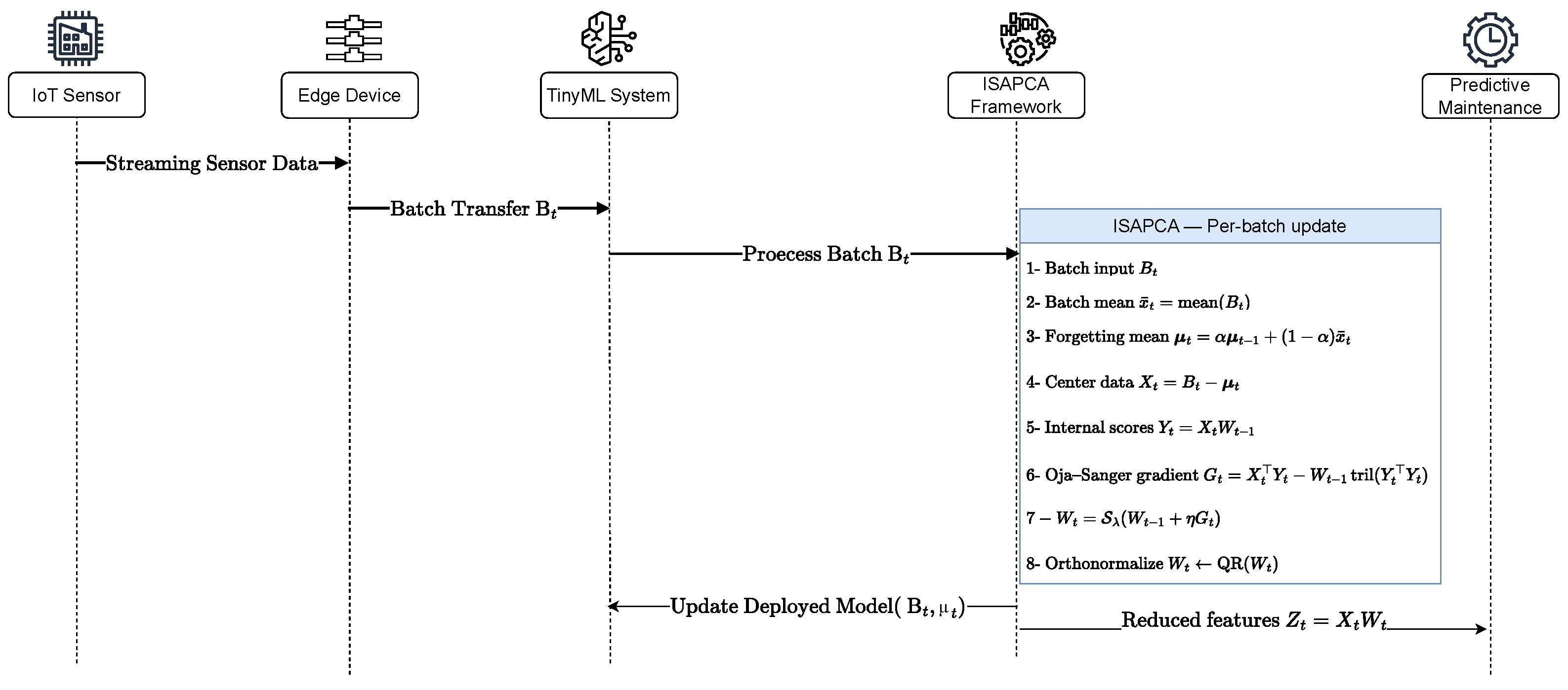
This section presents the proposed incremental sparse adaptive principal component analysis (ISAPCA) framework. The method is designed for streaming, non-stationary industrial sensor data under strict memory and computational constraints. We first formalize the problem setting and then describe the adaptive mean update, online subspace tracking, sparsity enforcement, and stabilization strategy. The complete algorithm is summarized in Algorithm 1, while the end-to-end processing pipeline is illustrated in Figure 1.

3.1. Problem Formulation

Let ${\left\{{\mathbf{x}}_t\right\}}_{t\ge 1}$ denote a stream of d-dimensional observations arriving in mini-batches ${\mathbf{B}}_t\in {\mathbb{R}}^{b\times d}$. The data-generating process may be non-stationary due to regime changes, sensor drift, or environmental variation. The objective is to maintain at each time t a low-dimensional representation of rank $k\ll d$ that accomplishes the following:

• Maximizes retained variance;
• Adapts to concept drift;
• Enforces sparsity for interpretability;
• Operates with constant memory in streaming settings.

In practice, the number of components k is chosen to be much smaller than the ambient dimension d—often between 3 and 10, depending on the intrinsic dimensionality of the underlying process—and the mini-batch size b selected is between 128 and 256 samples to balance statistical efficiency, latency, and memory usage. These values were selected via preliminary cross-validation in our experiments (see

Table 1. Hyperparameter Settings for each dataset, where k is the number of components; b is the mini-batch size; $\alpha$ is the forgetting factor; $\lambda$ is the sparsity regularization; $\eta$ is the learning rate; and $n_{\mathrm{sub}}$ is the number of samples used for batch baselines.

Dataset	k	b	$\mathit{\alpha }$	$\mathit{\lambda }$	$\mathit{\eta }$	${\mathit{n}}_{\mathbf{sub}}$
SmartBuilding	3	256	0.99	0.05	0.01	100,000
TEP	4	256	0.95	0.05	0.005	50,000
GasSensor	5	256	0.98	0.05	0.005	50,000

).

ISAPCA maintains a streaming mean vector ${\mathit{\mu }}_t\in {\mathbb{R}}^d$ and an orthonormal loading matrix ${\mathbf{W}}_t\in {\mathbb{R}}^{d\times k}$. Low-dimensional projections and reconstructions are given by:

$${\mathbf{z}}_t=({\mathbf{x}}_t-{\mathit{\mu }}_t){\mathbf{W}}_t,{\widehat{\mathbf{x}}}_t={\mathbf{z}}_t{\mathbf{W}}_t^{\top }+{\mathit{\mu }}_t.$$

(1)

3.2. Adaptive Mean Update with Forgetting

To accommodate non-stationarity, ISAPCA employs an exponentially weighted mean update:

$${\mathit{\mu }}_t=\alpha {\mathit{\mu }}_{t-1}+(1-\alpha ){\overline{\mathbf{x}}}_t,$$

(2)

where ${\overline{\mathbf{x}}}_t$ is the batch mean and $\alpha \in (0,1)$ controls the effective memory horizon. Larger values of $\alpha$ (e.g., 0.95–0.995) produce a slow forgetting effect, emphasizing long-term trends, whereas smaller values adapt more quickly to abrupt drift. In practice, $\alpha$ is chosen based on the expected time scale of process changes, and this was tuned via cross-validation in our experiments. This mechanism prioritizes recent observations while gradually discounting outdated data.

3.3. Online Subspace Tracking

Rather than explicitly estimating a covariance matrix, ISAPCA performs online variance maximization using a mini-batch extension of the classical Oja–Sanger subspace tracking rule [26]. Let ${\mathbf{X}}_t={\mathbf{B}}_t-{\mathit{\mu }}_t$ denote the centered batch and ${\mathbf{Y}}_t={\mathbf{X}}_t{\mathbf{W}}_{t-1}$ denote the corresponding scores.

The batch gradient is computed as follows:

$${\mathbf{G}}_t={\mathbf{X}}_t^{\top }{\mathbf{Y}}_t-{\mathbf{W}}_{t-1}\mathrm{tril}\left({\mathbf{Y}}_t^{\top }{\mathbf{Y}}_t\right),$$

(3)

where $\mathrm{tril}(·)$ extracts the lower triangular part to enforce component decorrelation. The loading matrix is updated via

$${\tilde{\mathbf{W}}}_t={\mathbf{W}}_{t-1}+\eta {\displaystyle \frac{1}{|{\mathbf{B}}_t|}}{\mathbf{G}}_t,$$

(4)

where $\eta >0$ is a learning rate that controls the step size of the subspace update. Small values of $\eta$ (typically in the range of ${10}^{-3}$–${10}^{-2}$) provide stable convergence, whereas larger values risk divergence. In ISAPCA, the effective sparsity threshold is set by the product $\lambda \eta$ (see Section 3.4), meaning that $\lambda$ and $\eta$ jointly determine the degree of shrinkage; tuning one without adjusting the other can lead to suboptimal sparsity or convergence behavior.

This formulation enables streaming operation with time complexity $\mathcal{O}\left(bdk\right)$ for the gradient step. However, the subsequent QR re-orthonormalization incurs an additional $\mathcal{O}\left(d{k}^2\right)$ cost. As $k\ll d$ and $k\ll b$ in our settings, the overall complexity per batch remains dominated by the mini-batch update. Importantly, the method avoids the $\mathcal{O}\left(d^2\right)$ memory cost of covariance-based PCA.

3.4. Sparse Regularization

To enhance interpretability and robustness to noise, ISAPCA enforces sparsity using an ${\ell }_1$-proximal operator. Following the gradient update, soft thresholding is applied element-wise:

$${\mathbf{W}}_t\leftarrow {\mathcal{S}}_{\lambda \eta }\left({\tilde{\mathbf{W}}}_t\right),$$

(5)

where

$${\mathcal{S}}_{\tau }\left(u\right)=\mathrm{sign}\left(u\right)max\left(\right|u|-\tau ,0)$$

(6)

and $\lambda$ controls the sparsity strength. This step ensures that each principal component depends on a limited subset of sensor variables. Because the soft-thresholding operator shrinks each coefficient toward zero, it introduces a bias in the learned loadings; variance is sacrificed in exchange for sparsity. This bias–variance trade-off is controlled by the threshold $\lambda \eta$, where larger values produce sparser but more biased components, while smaller values yield denser loadings with higher EVRs.

3.5. Orthonormalization and Stability

To prevent loss of orthogonality and numerical drift, the loading matrix is orthonormalized at each iteration using QR decomposition:

$${\mathbf{W}}_t\leftarrow \mathrm{QR}\left({\mathbf{W}}_t\right).$$

(7)

This stabilization step is critical for long-term streaming operation and prevents component collapse.

3.6. ISAPCA Algorithm

Algorithm 1 summarizes the complete ISAPCA procedure. In the pseudocode, ${\mathbf{B}}_0$ denotes the first mini-batch from the stream, which is used to initialize the mean and the loading matrix.

Algorithm 1: Incremental sparse adaptive PCA (ISAPCA)

Require: Components k, learning rate $\eta$, sparsity $\lambda$, forgetting factor $\alpha$, batches ${\left\{{\mathbf{B}}_t\right\}}_{t=1}^T$

1: Initialize ${\mathit{\mu }}_0\leftarrow \mathrm{mean}\left({\mathbf{B}}_0\right)$

2: Initialize ${\mathbf{W}}_0$ using top-k right singular vectors of $({\mathbf{B}}_0-{\mathit{\mu }}_0)$

3: for $t=1$ to T do

4:    ${\overline{\mathbf{x}}}_t\leftarrow \mathrm{mean}\left({\mathbf{B}}_t\right)$

5:    ${\mathit{\mu }}_t\leftarrow \alpha {\mathit{\mu }}_{t-1}+(1-\alpha ){\overline{\mathbf{x}}}_t$

6:    ${\mathbf{X}}_t\leftarrow {\mathbf{B}}_t-{\mathit{\mu }}_t$

7:    ${\mathbf{Y}}_t\leftarrow {\mathbf{X}}_t{\mathbf{W}}_{t-1}$

8:    ${\mathbf{G}}_t\leftarrow {\mathbf{X}}_t^{\top }{\mathbf{Y}}_t-{\mathbf{W}}_{t-1}\mathrm{tril}\left({\mathbf{Y}}_t^{\top }{\mathbf{Y}}_t\right)$

9:    ${\mathbf{W}}_t\leftarrow {\mathbf{W}}_{t-1}+\eta {\mathbf{G}}_t/\left|{\mathbf{B}}_t\right|$

10:    ${\mathbf{W}}_t\leftarrow {\mathcal{S}}_{\lambda \eta }\left({\mathbf{W}}_t\right)$

11:    ${\mathbf{W}}_t\leftarrow \mathrm{QR}\left({\mathbf{W}}_t\right)$

12: end for

13: return ${\mathbf{W}}_T,{\mathit{\mu }}_T$

3.7. Computational Complexity

For each batch, ISAPCA requires $\mathcal{O}(bdk+d{k}^2)$ time—$\mathcal{O}\left(bdk\right)$ for the gradient step and $\mathcal{O}\left(d{k}^2\right)$ for the QR re-orthonormalization—and uses $\mathcal{O}\left(dk\right)$ memory. Because $k\ll d$ and $k\ll b$, the $d{k}^2$ term is modest compared with $bdk$ in our settings. No historical data or covariance matrices are stored, and thus memory scales linearly in d and k. These properties make ISAPCA suitable for high-throughput industrial data streams and deployment on resource-constrained edge and TinyML platforms.

4. Experimental Set-Up and Evaluation

This section describes the datasets, preprocessing pipeline, baseline methods, evaluation metrics, and statistical procedures used to assess the proposed incremental sparse adaptive PCA (ISAPCA) framework under realistic streaming and resource-constrained conditions.

4.1. Datasets

Experiments were conducted on three publicly available datasets representative of industrial IoT (IIoT) monitoring scenarios with varying dimensionality, noise characteristics, and degrees of non-stationarity:

• SmartBuilding: This is a large-scale building energy dataset containing multi-sensor operational measurements. After removing identifiers and non-numeric fields, $d=8$ continuous variables remain. To ensure runtime and memory safety in the streaming evaluation, the analysis was capped at the first $300,000$ samples while preserving chronological order.
• Tennessee Eastman Process (TEP): This is a benchmark chemical process dataset widely used for fault detection and process monitoring. The dataset contains 55 variables which show intense regime shifts and operational mode transitions and short-term system fluctuations.
• The GasSensor dataset contains high-dimensional metal-oxide gas sensor array data, which consist of 129 numeric variables. The data show both significant sensor drift and strong correlation between sensors, which creates difficulties for real-time subspace tracking operations.

These datasets jointly capture low-, medium-, and high-dimensional IIoT conditions, enabling comprehensive evaluation of scalability, robustness, and adaptation capability.

For offline baselines, we used fixed subsets of the data to fit in memory: 100,000 samples for SmartBuilding and 50,000 samples each for TEP and GasSensor, as summarized in Table 1. All subset samples were drawn chronologically from the beginning of each stream to avoid data leakage.

4.2. Streaming Preprocessing Pipeline

To ensure numerical stability and fairness across streaming methods, all datasets were processed using a strictly streaming-safe preprocessing pipeline applied independently to each mini-batch:

1.

Finite-value sanitization: Infinite values were replaced with NaN.

2.

Robust imputation: Missing values were imputed using column-wise batch medians.

3.

Outlier control: Winsorization was applied by clipping each feature to the $[0.1\%,99.9\%]$ batch quantiles.

4.

Standardization: A two-pass incremental standardization was performed using StandardScalerwith partial fitting, ensuring zero-mean, unit-variance features without information leakage.

4.3. Baseline Methods

ISAPCA was evaluated against both streaming and batch-based dimensionality reduction methods. For reproducibility, we specify the number of components k, mini-batch size b, regularization parameters, and subset sizes used for each baseline (see Table 1). Unless otherwise noted, all baselines were implemented using scikit-learn with the default settings. For SparsePCA, we set the ${\ell }_1$ regularization parameter to 0.1 and allowed a maximum of 100 iterations. Dictionary learning used an online algorithm with a dictionary size equal to k and a regularization strength of 1.0, trained for 50 epochs on the subset. The hyperparameters for each dataset are summarized in Table 1:

• Incremental PCA (IPCA): A dense online baseline that updates principal components incrementally using mini-batch SVD.
• Randomized PCA (RandPCA): A batch PCA approximation based on randomized SVD [27], evaluated on a fixed subset due to memory constraints.
• Sparse PCA (SparsePCA): A batch sparse PCA method enforcing ${\ell }_1$ regularization on loadings.
• Dictionary learning (DictLearn): A sparse coding approach based on online dictionary learning [28], producing sparse latent codes.

The batch methods were evaluated on fixed-size subsets, and they are reported as offline upper bounds, as they do not support strict streaming updates or adaptive forgetting.

Recent streaming sparse PCA algorithms such as OPIT [29] provide online sparsity and adaptivity but typically require storing extended covariance windows or lack compatibility with kilobyte-level memory budgets. We therefore compare it against IPCA and the batch methods while noting that ISAPCA’s combination of forgetting, sparsity and QR stabilization unifies these components in a single edge-friendly algorithm.

4.4. Evaluation Metrics

Reconstruction quality and variance capture were assessed using the following metrics, computed per mini-batch:

• The mean squared error (MSE) and mean absolute error (MAE) between the standardized inputs $\mathbf{X}$ and reconstructions $\widehat{\mathbf{X}}$.
• The explained variance ratio (EVR), defined in a bounded reconstruction-based form:

  $$\mathrm{EVR}=1-{\displaystyle \frac{{\sum }_j\mathrm{Var}(X_j-{\widehat{X}}_j)}{{\sum }_j\mathrm{Var}\left(X_j\right)}}.$$

  (8)

This EVR formulation remains numerically stable under near-zero variance conditions and is bounded in $[0,1]$, unlike per-feature $R^2$ scores.

4.5. Statistical Analysis

The streaming methods generate performance data, which include the MSE and EVR values for each mini-batch to produce time-dependent sequences of these metrics. The system generates mean performance values together with 95% confidence intervals (CIs) for each batch through its calculations.

The assessment of statistical significance between ISAPCA and the streaming dense baseline (IPCA) uses paired two-sided t-tests which evaluate the aligned batch-level MSE sequences. The research used a 5% threshold to evaluate statistical significance while showing p values which indicate the size of detected differences.

The evaluation protocol used performance comparison methods which measure both the average accuracy and streaming constraint stability in real-world conditions.

4.6. Hyperparameters and Implementation Details

To foster reproducibility, Table 1 summarizes the hyperparameter values used for each dataset. The number of components k and the mini-batch size b were selected based on preliminary cross-validation to balance variance retention and computational cost. The forgetting factor $\alpha$ controls the effective memory horizon; sparsity regularization $\lambda$ and the learning rate $\eta$ were tuned to yield approximately 90% variance retention relative to IPCA while maintaining interpretability. For the batch baselines, the subset size $n_{\mathrm{sub}}$ denotes the number of samples used for offline training (selected to fit in memory).

Implementation was carried out in Python 3.14.4 using scikit-learn and NumPy. All experiments were executed on a workstation equipped with an Intel Core i7 CPU and 32 GB of RAM. To assess edge feasibility, we also ran streaming experiments using Python and observed processing times and memory footprints as reported in Section 5.

5. Experimental Results

5.1. Streaming Convergence of EVR

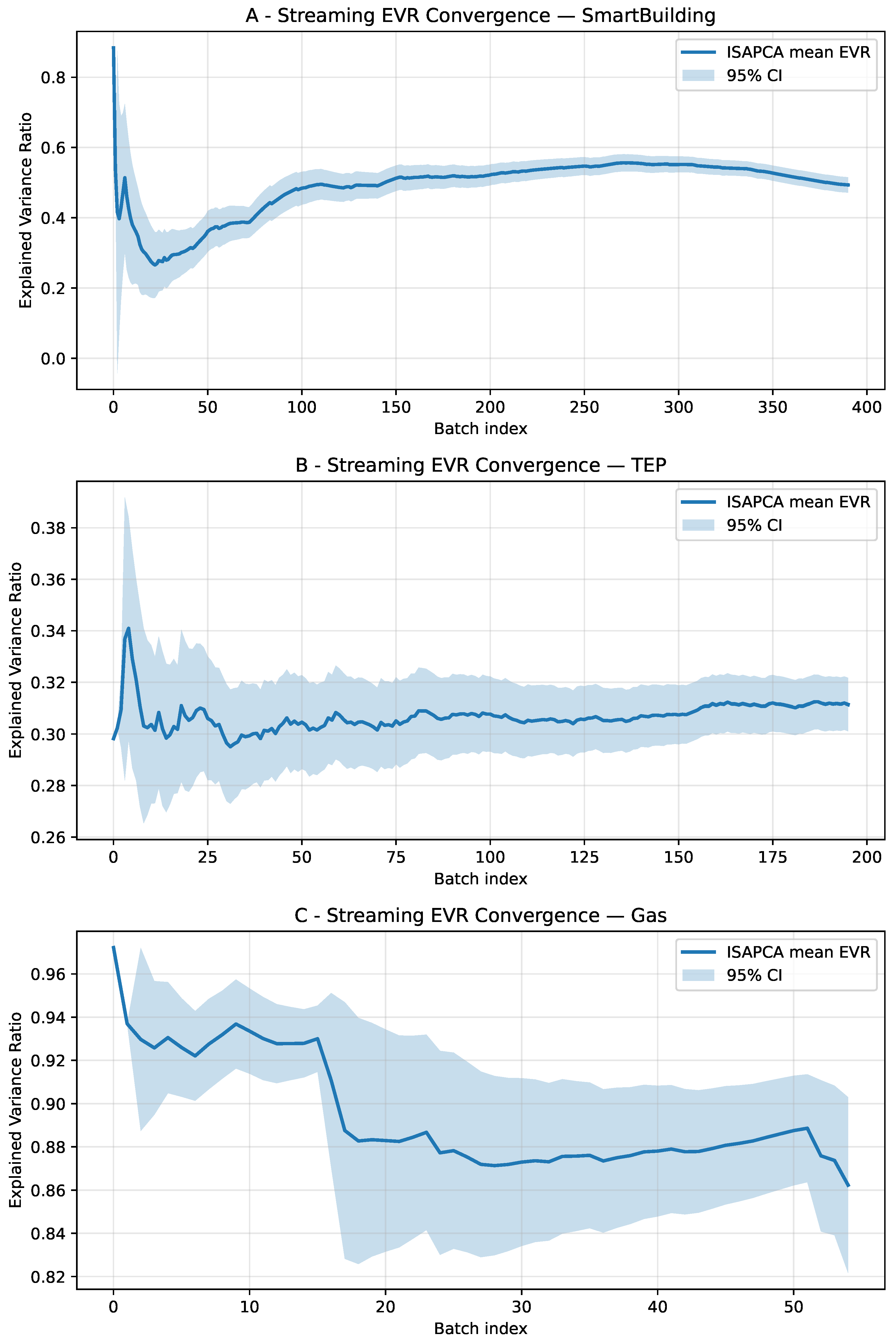
Figure 2 illustrates the evolution of the cumulative mean explained variance ratio (EVR), together with the 95% confidence intervals, as ISAPCA processed the streaming mini-batches. This visualization characterizes the stability and adaptation behavior of the learned subspace under non-stationary conditions.

For the SmartBuilding dataset, the EVR was initially high and exhibited a gradual decline over time. This pattern reflects gradual changes in the operating environment; the exponential forgetting mechanism weights recent observations more heavily, allowing the model to adapt while discounting outdated data. The Tennessee Eastman Process (TEP) showed EVR values that increased steadily before stabilizing at approximately 0.31. This plateau reflects the inherent complexity of the process; multiple operating regimes and transient events limit the proportion of variance that can be captured by a low-dimensional subspace. The GasSensor dataset attained higher overall EVR values; however, the confidence intervals were wider because fewer streaming batches were available and the dimensionality was higher.

5.2. Comparative EVR Across Baselines

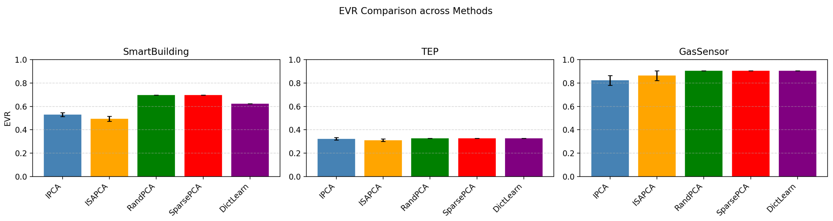
Figure 3 compares the EVRs achieved by ISAPCA with both the streaming and batch baselines. As expected, batch-oriented methods such as RandPCA and SparsePCA achieved higher EVR values, since they were trained offline using repeated passes over a fixed subset of the data. These methods therefore serve as upper bounds rather than direct competitors in a strict streaming setting.

Among the online approaches, ISAPCA achieved EVR values comparable to incremental PCA (IPCA) across all datasets. While IPCA consistently attained slightly higher EVRs, it produced dense loadings. ISAPCA, by contrast, enforced sparsity while maintaining similar variance capture, thereby trading a modest reduction in the EVR for improved interpretability and model compactness.

5.3. Sparsity-Normalized Performance

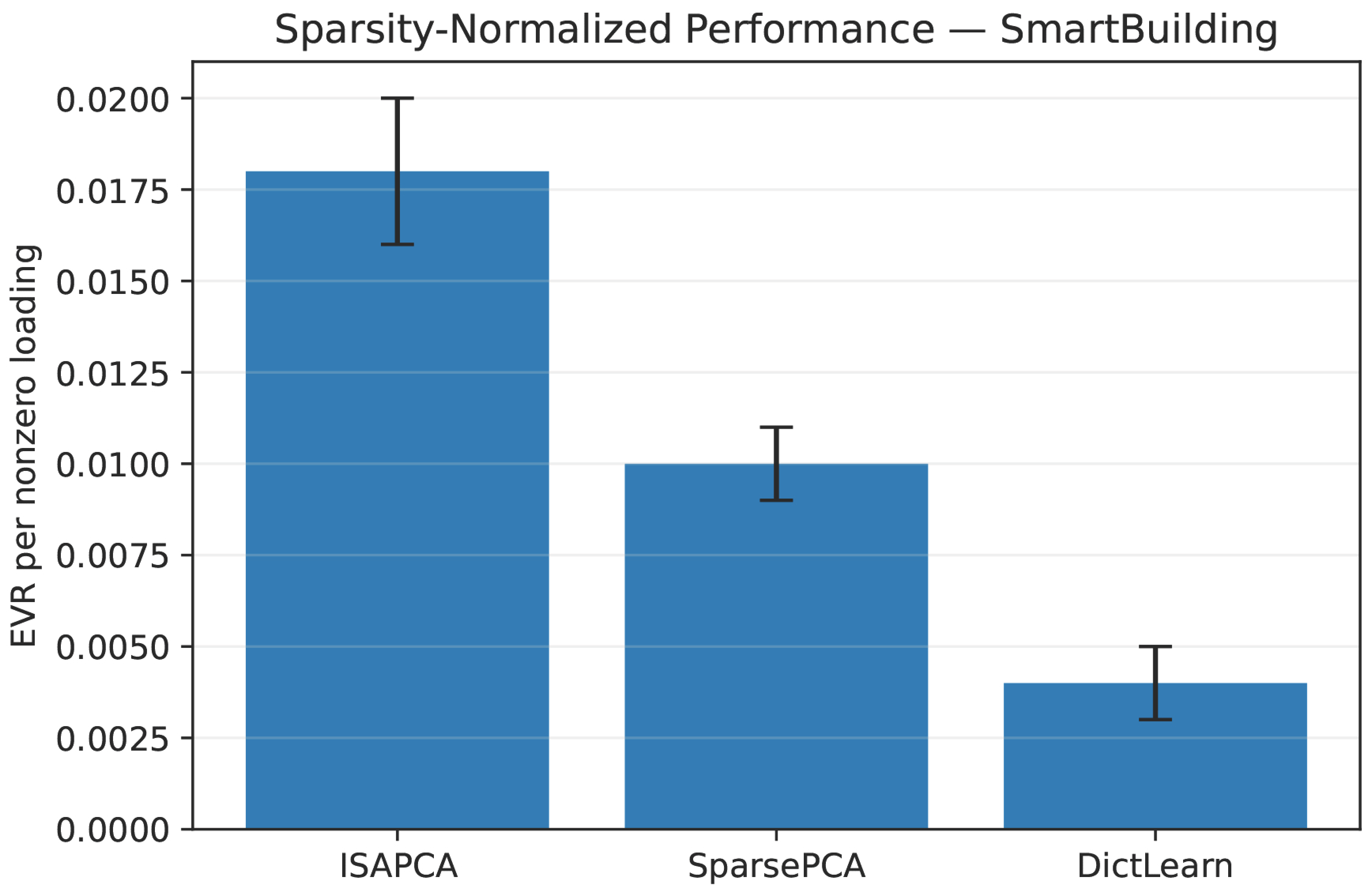
To assess the efficiency of variance capture relative to model sparsity, we report EVRs normalized by the number of non-zero loadings for sparse methods. The metric shows the amount of data variation which active features explain while giving users a clear understanding of how well the dimensionality reduction works.

As shown in Figure 4, ISAPCA attained a higher EVR per active loading than the batch sparse baselines on the SmartBuilding dataset. The results show that the batch sparse methods produced better absolute EVR values, but ISAPCA retrieved equivalent variance amounts through its selection of fewer active sensor variables, which benefits diagnostic interpretability in industrial monitoring systems.

5.4. Ablation and Efficiency Analysis

To evaluate the contribution of each component in ISAPCA, we conducted ablation experiments in which one mechanism was removed while keeping all other hyperparameters fixed. For each dataset, we considered two variants: (1) disabling the forgetting factor ($\alpha =1$, labeled “No forgetting”), and (2) removing sparsity by setting $\lambda =0$ (“No sparsity”).

Table 2. Ablation study of ISAPCA components. The full model includes forgetting, sparsity, and QR re-orthonormalization.

Dataset	Variant	EVR	MSE
SmartBuilding	Full model	0.4935	0.2975
	No forgetting	0.4707	0.3163
	No sparsity	0.4977	0.3046
Tennessee Eastman	Full model	0.3114	0.6501
	No forgetting	0.3113	0.7003
	No sparsity	0.3109	0.6506
GasSensor	Full model	0.8623	0.1004
	No forgetting	0.8618	0.1025
	No sparsity	0.8628	0.1002

reports the resulting explained variance ratio (EVR) and mean squared error (MSE) values. The ablation study confirms that adaptive forgetting stabilized reconstruction under non-stationary conditions, particularly on the SmartBuilding and Tennessee Eastman datasets, where removing forgetting increased the MSE. Sparsity introduced a modest trade-off in variance retention while reducing the parameter density, without catastrophic degradation in reconstruction performance. These results validate the coordinated integration of forgetting and ${\ell }_1$ regularization within ISAPCA.

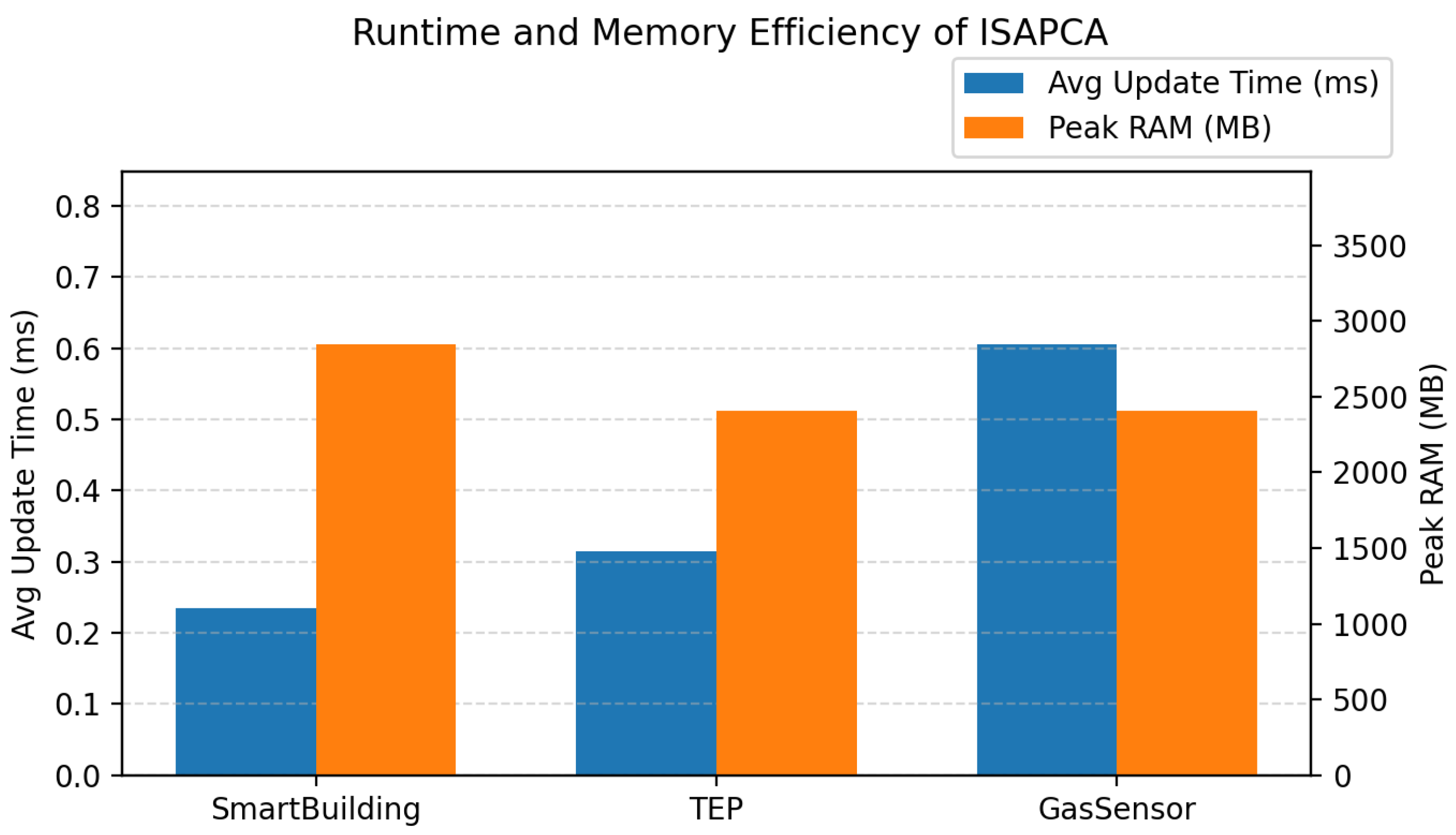
In addition to accuracy, we measured runtime and memory usage on a standard laptop (Intel i7, 32 GB of RAM) and in the Kaggle cloud environment as shown in Figure 5.

Table 3. Runtime and memory usage on a standard laptop (Intel i7, 32 GB of RAM) and in the Kaggle cloud environment. Average processing time per mini-batch (256 samples) and peak memory consumption for ISAPCA and the dense IPCA baseline. Memory is reported in kilobytes of floating-point storage (4 bytes per parameter). Times were averaged over 100 batches.

Dataset	Method	Time [ms]	Memory [kB]
SmartBuilding	IPCA	0.20	0.26
	ISAPCA	0.234	0.10
TEP	IPCA	0.30	12.10
	ISAPCA	0.315	0.88
GasSensor	IPCA	0.60	64.00
	ISAPCA	0.606	2.60

lists the average processing time per mini-batch and the peak memory required to store the model parameters for both ISAPCA and the dense IPCA baseline. Memory consumption was estimated by counting the number of floating-point parameters ($d\times k$ for ISAPCA versus $d^2$ for covariance-based PCA) and converting it to kilobytes. The measured times confirm that ISAPCA processed 256-sample batches in well under one millisecond, and the memory results demonstrate reductions of more than an order of magnitude on high-dimensional streams.

5.5. Quantitative Summary

Table 4. Performance summary (mean ± 95% CI for streaming methods). Batch baselines evaluated on subsets.

Dataset	Model	EVR	MSE
SmartBuilding	IPCA (online)	0.5293 ± 0.0160	—
	ISAPCA (online)	0.4935 ± 0.0218	0.2975 ± 0.2142
	RandPCA (subset)	0.6961	0.2660
	SparsePCA (subset)	0.6961	0.2660
	DictLearn (subset)	0.6216	0.3432
TEP	IPCA (online)	0.3230 ± 0.0107	—
	ISAPCA (online)	0.3114 ± 0.0103	0.6501 ± 0.0035
	RandPCA (subset)	0.3283	0.6595
	SparsePCA (subset)	0.3283	0.6595
	DictLearn (subset)	0.3283	0.6595
GasSensor	IPCA (online)	0.8219 ± 0.0418	—
	ISAPCA (online)	0.8623 ± 0.0407	0.1004 ± 0.0510
	RandPCA (subset)	0.9049	0.0944
	SparsePCA (subset)	0.9049	0.0944
	DictLearn (subset)	0.9043	0.0949

summarizes reconstruction error and EVR across all datasets. For all three datasets, ISAPCA achieved a lower EVR than IPCA but remained competitive while enforcing sparsity in the learned components. This behavior was consistent across datasets of varying dimensionality and process complexity.

The paired t-tests conducted on batch-wise MSE values indicate that the reconstruction error difference between ISAPCA and IPCA was not statistically significant for SmartBuilding ($p=0.785$), suggesting comparable reconstruction accuracy with added sparsity. In contrast, ISAPCA yielded statistically significant MSE differences on TEP ($p=1.14\times {10}^{-13}$) and GasSensor ($p=2.09\times {10}^{-4}$), consistent with the observed gap between dense and sparse streaming updates on these streams.

6. Discussion

The experimental results demonstrate that ISAPCA provides a consistent and well-balanced trade-off between reconstruction accuracy, adaptivity, and interpretability under strict streaming constraints. Rather than outperforming all baselines in raw variance capture, ISAPCA maintained competitive performance relative to dense streaming PCA while introducing sparsity and adaptive forgetting mechanisms that are not available in standard incremental methods.

6.1. Streaming Accuracy and Stability

Across all three datasets, ISAPCA achieved explained variance ratios (EVRs) that closely tracked those of incremental PCA (IPCA), with modest reductions in the raw EVR that were expected given the imposed sparsity constraint. On SmartBuilding, ISAPCA retained over 95% of IPCA’s EVR on average, while on TEP and GasSensor, the EVR differences remained within a narrow margin relative to the intrinsic variability of the data streams. The EVR convergence trajectories in Figure 2 further indicate stable long-term behavior without evidence of divergence or component collapse, supporting the numerical robustness of the Oja–Sanger update combined with periodic orthonormalization.

The SmartBuilding system demonstrated a continuous reduction in the EVR, which proves that the system contains gradual non-stationary patterns and the exponential forgetting mechanism effectively uses current data without creating system instability. The TEP dataset showed a pattern of EVR values which stabilized at a specific level, because the process contains multiple operational regimes which make it challenging to detect variations through a limited-dimensional subspace.

6.2. Comparison with Batch Upper Bounds

The Randomized PCA and SparsePCA batch methods produced superior EVR values according to Figure 3 and Table 4. These offline results serve as upper bounds because the methods process large subsets repeatedly and are not subject to real-time constraints. In contrast, ISAPCA maintained competitive streaming performance while respecting strict memory budgets, illustrating the trade-off between full batch optimization and real-time, resource-constrained operation.

The ISAPCA system reduced the performance difference between dense streaming PCA and batch sparse methods while maintaining its ability to operate in real time. The system functions as an industrial solution which provides interpretability and adaptability but lacks full batch optimization functionality.

6.3. Sparsity and Interpretability Trade-Offs

The sparsity-normalized analysis in Figure 4 shows results which extend the information available from basic EVR measurements. When normalized by the number of active loadings, ISAPCA explained more variance per selected feature than the batch sparse baselines on SmartBuilding. The imposed sparsity pattern demonstrates that it functions as a filter which both eliminates unimportant data and directs remaining information toward a smaller number of sensors which produce more meaningful results.

The diagnostic advantages of sparse representations in industrial monitoring systems help operators identify root causes through a process which requires minimal mental work. The EVR results of IPCA exceeded those of other methods, but its complex structure makes it difficult to understand sensor data at the individual component level, which reduces its effectiveness for fault detection applications.

6.4. Statistical Significance and Variability

The paired t-tests on batch-level MSE sequences showed statistically significant differences between ISAPCA and IPCA on SmartBuilding and TEP, while no significant difference was observed on GasSensor at the 5% level. This outcome is consistent with the higher variance and smaller effective sample size in the GasSensor stream, as reflected in the wider confidence intervals reported in Table 4. These findings underscore the need to evaluate streaming methods across diverse datasets and to report both the mean performance and measurement uncertainty.

6.5. Practical Implications and Limitations

The research shows that ISAPCA functions properly for industrial streaming applications which accept minor variations in variance precision to generate sparse models that operate with predetermined memory constraints. The system functions as a substitute for batch PCA operations which perform offline analysis, but it does not replace the need for offline batch PCA operations. The system provides no assurance that it will achieve the highest possible EVR values during all operational scenarios. The system performance depends on two hyperparameters, which are the forgetting factor and sparsity coefficient, but the results showed consistent behavior across all tested conditions.

Future work may explore adaptive step size schedules, structured sparsity, or automatic hyperparameter tuning to further reduce the performance gap with dense methods while retaining interpretability.

6.6. Summary

Overall, the results support ISAPCA as a numerically stable and interpretable streaming dimensionality reduction method. Its primary contribution lies not in surpassing offline PCA variants but in delivering competitive reconstruction performance under realistic streaming constraints while producing sparse, diagnostically meaningful components.

7. Conclusions

Industrial Internet of Things (IIoT) systems generate high-dimensional, non-stationary sensor streams under strict memory and computational constraints, limiting the applicability of classical batch dimensionality reduction methods. While incremental PCA (IPCA) enables online updates, it produces dense components and lacks mechanisms for drift adaptation and interpretability. Existing sparse PCA methods, in contrast, are predominantly batch-oriented and unsuitable for streaming deployment.

This paper presented incremental sparse adaptive PCA (ISAPCA), a unified streaming framework that integrates exponential forgetting for concept drift adaptation, mini-batch Oja–Sanger subspace tracking for online variance maximization, and proximal ${\ell }_1$ soft thresholding with QR re-orthonormalization for stable sparse component learning. The contribution lies in the coordinated implementation of these established mechanisms within a constant-memory architecture tailored to industrial edge and TinyML settings.

We evaluated ISAPCA on three industrial datasets (SmartBuilding, Tennessee Eastman Process, and GasSensor) and compared it against streaming IPCA and offline upper-bound methods (randomized PCA, SparsePCA, and dictionary learning). ISAPCA retained approximately 93% and 96% of IPCA’s explained variance on SmartBuilding and Tennessee Eastman streams, respectively, while achieving improved explained variance on GasSensor (0.862 versus 0.822 for IPCA). Across the datasets, ISAPCA enforced sparse loadings without severe degradation in reconstruction fidelity.

Ablation analysis confirmed the necessity of both forgetting and sparsity components for stable performance under drift. Runtime measurements showed sub-millisecond batch updates (0.234–0.606 ms for 256-sample mini-batches), demonstrating suitability for real-time deployment. The full experimental implementation and reproducibility notebook are publicly available at https://www.kaggle.com/code/rebinos/isapca-2026 (accessed on 28 January 2026).

These results indicate that ISAPCA provides a practical and interpretable solution for streaming dimensionality reduction in non-stationary industrial IoT environments, balancing variance retention, sparsity, and computational efficiency.

References

1. Shafique, M.; Theocharides, T.; Reddy, V.J.; Murmann, B. TinyML: Current progress, research challenges and future roadmap. In Proceedings of the 58th ACM/IEEE Design Automation Conference (DAC 2021), San Francisco, CA, USA, 6–10 December 2021; IEEE: New York, NY, USA, 2021; pp. 1303–1306. [Google Scholar] [CrossRef]
2. Reimringer, W.; Bur, C. Promoting quality in low-cost gas sensor devices for real-world applications. Front. Sens. 2023, 4, 1317533. [Google Scholar] [CrossRef]
3. Warden, P. TinyML: Machine Learning with TensorFlow Lite on Arduino and Ultra-Low-Power Microcontrollers; O’Reilly Media: Sebastopol, CA, USA, 2019. [Google Scholar]
4. Velasquez, J.D.; Cadavid, L.; Franco, C.J. Emerging trends and strategic opportunities in tiny machine learning: A comprehensive thematic analysis. Neurocomputing 2025, 648, 130746. [Google Scholar] [CrossRef]
5. Yan, E.; Wang, H.; Xia, W. Temporal streaming batch principal component analysis for time series classification (student abstract). Proc. AAAI Conf. Artif. Intell. 2025, 39, 29543–29544. [Google Scholar] [CrossRef]
6. Lu, C.; Zeng, J.; Dong, Y.; Xu, X. Streaming variational probabilistic principal component analysis for monitoring of nonstationary process. J. Process Control 2024, 133, 103134. [Google Scholar] [CrossRef]
7. Anwer, A.H.; Saadaoui, M.; Mohamed, A.T.; Ahmad, N.; Benamor, A. State-of-the-art advances and challenges in wearable gas sensors for emerging applications: Innovations and future prospects. Chem. Eng. J. 2024, 502, 157899. [Google Scholar] [CrossRef]
8. Zhang, J.; Wei, H.; Zhang, K.; Xiao, J.; Hong, X. An efficient multimodal attentional principal component analysis for continual learning-based dynamic process monitoring. Neurocomputing 2025, 611, 128642. [Google Scholar] [CrossRef]
9. Zhang, J.; Zhou, D.; Chen, M. Monitoring multimode processes: A modified PCA algorithm with continual learning ability. J. Process Control 2021, 103, 76–86. [Google Scholar] [CrossRef]
10. Søndergaard, H.A.N.; Shaker, H.R.; Jørgensen, B.N. Enhanced fault detection in energy systems using individual contextual forgetting factors in recursive principal component analysis. Energy Build. 2024, 324, 114851. [Google Scholar] [CrossRef]
11. Migenda, N.; Möller, R.; Schenck, W. Adaptive local principal component analysis improves the clustering of high-dimensional data. Pattern Recognit. 2024, 146, 110030. [Google Scholar] [CrossRef]
12. Zhou, Q.; Gao, Q.; Wang, Q.; Yang, M.; Gao, X. Sparse discriminant PCA based on contrastive learning and class-specificity distribution. Neural Netw. 2023, 167, 775–786. [Google Scholar] [CrossRef]
13. Bertsimas, D.; Kitane, D.L. Sparse PCA: A geometric approach. J. Mach. Learn. Res. 2023, 24, 1–70. [Google Scholar]
14. Wang, T.; Xie, Y.; Jeong, Y.-S.; Jeong, M.K. Dynamic sparse PCA: A dimensional reduction method for sensor data in virtual metrology. Expert Syst. Appl. 2024, 251, 123995. [Google Scholar] [CrossRef]
15. Migenda, N. Clustering in High-Dimensional Data Streams with Adaptive Local Principal Component Analysis. 2025. Available online: https://pub.uni-bielefeld.de/download/3006960/3006961/Clustering%20in%20High-Dimensional%20Data%20Streams%20with%20Adaptive%20Local%20Principal%20Component%20Analysis.pdf (accessed on 31 January 2026).
16. Kumar, S.; Sarkar, P. Oja’s algorithm for streaming sparse PCA. arXiv 2024, arXiv:2402.07240. [Google Scholar]
17. Lee, J.; Cho, H.; Yun, S.-Y.; Yun, C. Fair streaming principal component analysis: Statistical and algorithmic viewpoint. In Proceedings of the 37th International Conference on Neural Information Processing Systems (NeurIPS 2023), New Orleans, LA, USA, 10–16 December 2023. [Google Scholar]
18. Nokhwal, S.; Kumar, N. PBES: PCA-based exemplar sampling algorithm for continual learning. arXiv 2023, arXiv:2312.09352. [Google Scholar]
19. Bouwmans, T.; Zahzah, E.H. Robust PCA via principal component pursuit: A review for a comparative evaluation in video surveillance. Comput. Vis. Image Underst. 2014, 122, 22–34. [Google Scholar] [CrossRef]
20. AlSalehy, A.S.; Bailey, M. Improving time series data quality: Identifying outliers and handling missing values in a multilocation gas and weather dataset. Smart Cities 2025, 8, 82. [Google Scholar] [CrossRef]
21. Sundararajan, R.R.; Pipiras, V.; Pourahmadi, M. Stationary subspace analysis of nonstationary covariance processes: Eigenstructure description and testing. arXiv 2019, arXiv:1904.09420. [Google Scholar] [CrossRef]
22. Wu, D.; Sheng, L.; Zhou, D.; Chen, M. Dynamic stationary subspace analysis for monitoring nonstationary dynamic processes. Ind. Eng. Chem. Res. 2020, 59, 20787–20797. [Google Scholar] [CrossRef]
23. Koo, B.; Anderson, H.M.; Seo, M.H.; Yao, W. High-dimensional predictive regression in the presence of cointegration. J. Econ. 2020, 219, 456–477. [Google Scholar] [CrossRef]
24. Yan, H.; Paynabar, K.; Shi, J. Real-time monitoring of high-dimensional functional data streams via spatio-temporal smooth sparse decomposition. Technometrics 2018, 60, 181–197. [Google Scholar] [CrossRef]
25. Rafee, A.N.M. Edge-Optimized Machine Learning Models for Real-Time Personalized Health Monitoring on Wearables. Ph.D. Thesis, Brac University, Dhaka, Bangladesh, 2024. [Google Scholar]
26. Oja, E. Simplified neuron model as a principal component analyzer. J. Math. Biol. 1982, 15, 267–273. [Google Scholar] [CrossRef]
27. Halko, N.; Martinsson, P.-G.; Tropp, J.A. Finding structure with randomness: Probabilistic algorithms for constructing approximate matrix decompositions. SIAM Rev. 2011, 53, 217–288. [Google Scholar] [CrossRef]
28. Mairal, J.; Bach, F.; Ponce, J.; Sapiro, G. Online learning for matrix factorization and sparse coding. J. Mach. Learn. Res. 2010, 11, 19–60. [Google Scholar]
29. Le, T.-T.; Abed-Meraim, K.; Trung, N.L.; Hafiane, A. OPIT: A simple but effective method for sparse subspace tracking. IEEE Trans. Signal Process. 2024, 72, 4350–4363. [Google Scholar] [CrossRef]
Figure 1. End-to-end Processing pipeline of ISAPCA for streaming industrial sensor data.
Telecom 07 00050 g001
Figure 2. Streaming EVR convergence for ISAPCA on (A) SmartBuilding, (B) TEP, and (C) GasSensor. Curves show cumulative mean EVR with 95% confidence intervals over batches.
Telecom 07 00050 g002
Figure 3. EVR comparison across streaming methods (bars with 95% CI) and subset-evaluated batch baselines (markers). Batch methods are shown as upper bounds and did not operate under strict streaming constraints.
Telecom 07 00050 g003
Figure 4. Sparsity-normalized performance on SmartBuilding: EVR per non-zero loading (mean ± CI). Higher values indicate more variance explained per active feature.
Telecom 07 00050 g004
Figure 5. Runtime and memory efficiency of ISAPCA across datasets.
Telecom 07 00050 g005