Comparison of Outdoor Radiowave Propagation Models for Land Mobile Systems in the 3.6 GHz and 6 GHz Frequency Bands

Abstract

This paper presents a comparative analysis of three outdoor wave propagation models—ITU-R P.1546-6, the SUI model, and ITU-R P.452-17—benchmarked against the deterministic Parabolic Equation Modeling (PEM) method at 3.6 GHz and 6 GHz. The evaluation focuses on prediction accuracy (RMSE, MAE, bias, relative error), terrain sensitivity, and computational efficiency. At 3.6 GHz, ITU-R P.1546-6 shows poor terrain responsiveness and high relative errors, while ITU-R P.452-17 demonstrates strong terrain sensitivity and low errors in flat areas, but decreased accuracy over hilly terrain. At 6 GHz, the SUI model consistently underestimates field strength and exhibits weak terrain sensitivity, limiting its use to rough estimations. In contrast, ITU-R P.452-17 maintains good terrain correlation and acceptable accuracy, although it slightly overestimates field strength in complex environments. The results confirm that prediction accuracy, terrain sensitivity, and bias are highly model- and frequency-dependent. ITU-R P.452-17 emerges as the most reliable and computationally efficient alternative to deterministic methods when terrain effects must be considered without significant computational overhead.

1. Introduction

The modeling of electromagnetic wave propagation plays a key role in the implementation, design, and operation of rapidly evolving wireless telecommunication systems. These wave propagation models aim to quickly and efficiently determine the path loss of the propagation medium with low computational complexity, thus opening up the possibility to design, build, and deploy telecommunication networks in a cost-effective way. Wave propagation models also play a key role in quickly and efficiently estimating the potential for interference between individual telecommunication systems and the exclusion distance required to minimize the probability of harmful interference without costly field measurements [1]. The generic set of wave propagation models is large and growing thanks to research on the subject. Given that these models are typically specific to frequency band, telecommunications service, terrain and weather conditions, and a myriad of other parameters, it requires care to choose the right one as a user.

With the rapid development of mobile telecommunication networks, newer and newer generation technologies require higher and higher frequency bands, which increase data transmission speeds, while at the same time, they are capable of covering smaller distances and areas per base station at a given power level. This technological development trend implies the need to revise the previously used wave propagation models and to develop new wave propagation models that are accurate for high-frequency mobile telecommunication networks and that simultaneously apply modern soft computing techniques [2].

In order to understand what wave propagation models do, it is worth formalizing the problem. A wave propagation model can be considered as a system with $n+m$ inputs and one output, describable by a $\Gamma \{·\}$ operator. The n inputs of the system describe the transmitter under investigation, while the m inputs describe the environmental parameters that affect the wave propagation characteristics, such as the terrain between the transmitter and the receiver, the weather conditions, and the vegetation conditions. It is not explicitly indicated in Figure 1, but it is emphasized that for most wave propagation models, the important parameter is the height above sea level and/or ground level of the receiving point, and its geolocation can be used to determine, for example, the terrain section referred to earlier.

The first n inputs, which depend on the transmitter parameters, can be considered as direct or external inputs to the system, while the remaining m inputs are internal, indirect parameters of the system, which are not directly related to the transmitter parameters. The wave propagation model as a system can therefore be formalized as follows:

$$\mathrm{PL}=\Gamma \left(k_1,k_2,\dots ,k_m\right)\left\{x_1,x_2,x_3,\dots ,x_n\right\}.$$

(1)

The number of wave propagation models used in network planning and spectrum engineering is large, but they can be divided into different categories depending on the internal behavior of the model, i.e., the $\Gamma \{·\}$ system operator in the example above. The first large category consists of empirical wave propagation models [3]. These models describe the propagation of electromagnetic waves in a given environment on a statistical basis, using relationships derived from measured data. The measurement data can be used directly, for example, to train a neural network-based empirical wave propagation model that, given a sufficiently large amount of measurement data, can quickly produce accurate results that match the measurement results using a simple algorithm [4,5]. Another typical approach in this category is the use of wave propagation curves or curve sets constructed from measured data, where the wave propagation model algorithm can determine the path loss associated with a given input parameter set by interpolation and/or extrapolation. One such empirical wave propagation model is ITU-R P.1546 [6], which is widely used and accepted in international interference calculations. In this paper, we will discuss in detail this empirical wave propagation model, which can be appropriately applied to the 3.6 GHz frequency band. Although the model was only applicable up to 3 GHz until its previous version [7], it has been extended to 4 GHz and is now considered a suitable model for this band.

A broad family of empirical models are those that do not work with curves built from measured data, but with closed mathematical formulas containing constants assigned to specific installation coverage, frequency bands of use, base and mobile station antenna heights, etc.

The empirical models thus provide fast and simple calculations that can be used effectively when planning radio networks or performing spectrum management tasks. Importantly, they do not explicitly model individual propagation phenomena (e.g., reflection, scattering, and diffraction), but are based on averaged environmental effects. They can be widely used in urban, rural, and even indoor environments, but their accuracy is limited to the range of the data measured, so they may not be precise when applied to other environments, and their use requires careful consideration. One of the best-known of this type is the Okumura–Hata model, which in its original form and constants is suitable for estimating path loss between 150 MHz and 1500 MHz. It was later extended to the 1500 MHz and 2000 MHz frequency ranges as the COST 231-Hata model [8,9]. Given that Mobile/Fixed Telecommunication Network (MFCN) systems are allocated in increasingly higher frequency bands, the need to retune these models has also opened up. This is possible, for example, by redefining the parameters of the Okumura–Hata and COST 231-Hata models using optimization algorithms in order to better fit the measurement results in the pioneer MFCN bands [10].

A similar model is the Stanford University Interim (SUI) model [11], which can be applied to higher frequencies than the COST 231-Hata model [12]. However, a research gap has been identified to tune this model more accurately for the 6 GHz frequency band in order to better fit the outdoor wave propagation properties of this frequency band than is given in its present form.

The second large group of wave propagation models regards deterministic wave propagation models. These models are based on mathematical equations describing the propagation of electromagnetic waves as a physical phenomenon, which can be derived from Maxwell’s equations. They provide accurate predictions with detailed and precise consideration of the terrain and environment, and are not frequency-specific. They have the disadvantage of being more computationally complex than empirical models, especially when considering larger areas and more advanced cases [13]. One such widely used method is the Parabolic Equation Modeling (PEM), which is based on the numerical evaluation of parabolic equations. It is mainly used for modeling long-range radio wave propagation and topography effects. The model is based on a special approximation of Maxwell’s equations [14]. Although in this paper we are dealing with PE, it is worth mentioning that there are many other deterministic models, among which the Ray Tracing method is widely used [15], as well as the Finite-Difference Time-Domain [16] (FDTD) and the Method of Moments [17] (MoM), noting that the last two are not typically used for long-range wave propagation problems due to the high computational capacity required.

It is important to point out that there are also so-called hybrid-type, i.e.,semi-empirical or semi-deterministic, wave propagation models, which combine the advantages and disadvantages of the two large groups, with specified compromises. In this paper, we consider the ITU-R P.452-17 wave propagation model [18], which can be used as a hybrid model for both the 3.6 GHz and 6 GHz frequency bands, as well as the 3GPP 38.901 model [19].

The comparison, advantages and disadvantages of each group of wave propagation models are shown in

Table 1. Comparison of wave propagation models.

Model Type	Advantages	Disadvantages
Empirical	Fast, efficient, widely used in planning; applicable in urban, rural, and indoor environments; adaptable via optimization.	Limited to measurement-based environments; does not model physical effects like reflection or diffraction.
Deterministic	High accuracy, considers terrain/environment, frequency-independent; models propagation effects precisely.	Computationally expensive; slow for large-scale simulations; complexity increases with environment details.
Hybrid	Combines empirical and deterministic benefits; balances efficiency and accuracy; supports broad frequencies.	Requires data calibration; more complex than empirical models but simpler than deterministic ones.

.

As mentioned earlier, in this paper, the analysis of wave propagation models is limited to outdoor wave propagation phenomena, mobile telecommunication networks, and two frequency bands, 3.4–3.8 GHz and 6 GHz. The 3.4–3.6 and 3.6–3.8 GHz frequency bands are globally allocated on a co-primary basis for mobile services, except for aeronautical mobile, according to the Radio Regulations (RR) [20]. According to the European Table of Frequency Allocations and Applications (ECA Table), both bands are allocated for mobile service, supporting their use for terrestrial mobile networks in Europe [21]. Based on European Commission Implementing Decisions [22,23], the 3.4–3.8 GHz frequency band has been harmonized for terrestrial systems capable of providing electronic communications services in the European Union, and the harmonized frequency arrangements as well as the least restrictive technical conditions for MFCN have been also defined in ECC Decision (11)06 [24]. All this has opened up the possibility of using the band for MFCN at the European level, so its investigation is relevant and justified.

The 6 GHz frequency band in Europe is currently mainly allocated for wireless access systems (WAS/RLAN). This applies in particular to the lower 6 GHz sub-band (below 6425 MHz), which has been designated for WAS/RLAN use in most European countries. The use of the 6 GHz band for mobile networks (e.g., 5G) is currently not widespread in Europe. In the upper part of the 6 GHz band (6425–7125 MHz), satellite services and long-distance point-to-point links are still in operation in many European countries. Within the relevant groups of ECC, there are ongoing studies investigating the possible use of the band [25], including scenarios of exclusive mobile use (e.g., 5G/6G) or shared use between WAS/RLAN and mobile networks in the 6425–7125 MHz range. However, there is currently no widespread implementation for mobile purposes. In contrast, countries such as the United States, Canada, Brazil, and Australia have authorized the use of the entire 6 GHz band for WAS/RLAN.

Given that the potential for mobile applications is open, it is useful and forward-looking to investigate the wave propagation models for the band for future network planning and interference analysis, and to develop new models as a research gap.

Based on the above,

Table 2. Classification of the wave propagation models considered in this article.

Model Type	3.6 GHz	6 GHz
Empirical	ITU-R P.1546-6 [6]	SUI Model [11,12]
Deterministic	Parabolic Equation Modeling [14]
Hybrid	ITU-R P.452-17 [18]

shows the wave propagation models considered in this paper, classified by type and frequency range.

2. The ITU-R P.1546-6 Wave Propagation Model

The internationally acknowledged and accepted wave propagation model, widely used for terrestrial services, including mobile telecommunications networks, is defined in ITU-R Recommendation P.1546-6: Method for point-to-area predictions for terrestrial services in the frequency range 30 MHz to 4000 MHz. This recommendation is maintained by the ITU-R WP 3K working group, responsible for point-to-area propagation in general [26]. This wave propagation model is purely empirical, based on a set of propagation curves based on the measured results [27], which are clustered at 100 MHz, 600 MHz, and 2000 MHz, taking into account several types of propagation paths (land, cold sea, and warm sea).

In the example curve series shown in Figure 2, the field strength levels are plotted as a logarithmic function of distance for a given frequency, propagation path type, $h_1$, and time percentage. The model is applicable in the frequency range from 30 MHz to 4000 MHz, requiring inter- and extrapolation between the 100 MHz, 600 MHz, and 2000 MHz curves. The maximum length of the propagation path is 1000 km. The type of propagation path can be terrestrial or sea, with a distinction being made between cold sea, warm sea, and general sea paths. The importance of the temperature distinction between sea types arises, for example, from the more frequent reporting of super-refraction in warm seas [28,29], which may result in paths with lower path loss than in cold seas. In general, it can also be concluded that due to the homogeneity of the water surface, lower path loss can be assumed for wave propagation over large, contiguous water surfaces.

In principle, $h_1$ is the effective height of the transmitting antenna, which depends primarily on the type (land, sea, or mixed) and length of the propagation path. For land paths, $\left(d\le 3 \mathrm{km}\right)$ is the height of the antenna above ground level for short distances, and for longer paths, it is the height relative to the surrounding terrain. For sea paths, the physical height above sea level is applicable, but the model is only reliable for antennas higher than 3 m. For mixed paths, values must be determined separately for each section and then combined by interpolation.

The time percentage is the percentage of the time that the real measured field strength level can exceed the calculated field strength level estimated by the model when looking at an average year [27]. To give a simple example: if the value determined by the model is 60 dB$\mu$V/m at 10% time, then for 36.5 days in 1 year, i.e., 876 h, the actual measured field strength level may exceed the calculated value, while for the remaining time, i.e., 7884 h, the maximum value is 60 dB$\mu$V/m.

The model performs interpolation and extrapolation between the propagation curves, except for the extreme values, according to the variables frequency $\left(f\right)$, distance $\left(d\right)$, and as $h_1$. This procedure is illustrated in Figure 3.

This method [30] is based on the principle of linear interpolation, which assumes a linear relationship between the independent variable $\left(x\right)$ and the dependent variable $\left(y\right)$. Let the inferior and the superior values of x be $x_{inf}$ and $x_{sup}$, and similarly, for the dependent variable $y_{inf}$ and $y_{sup}$. For a given $x_{inf}\le x_0\le x_{sup}$, the task is to find $y_{inf}\le y_0\le y_{sup}$, such that we know that the x-derivative of y is constant due to the linear relationship. From this,

$${\displaystyle \frac{\Delta y}{\Delta x}}={\displaystyle \frac{y_0-y_{inf}}{x_0-x_{inf}}}={\displaystyle \frac{y_{sup}-y_{inf}}{x_{sup}-x_{inf}}}\iff y_0=y_{inf}+{\displaystyle \frac{\left(y_{sup}-y_{inf}\right)\left(x_0-x_{inf}\right)}{x_{sup}-x_{inf}}}.$$

(2)

Considering the wide range of interpretation of the variables, it is appropriate to proceed to logarithmic scaling, which leads to the following relationship:

$$y_0=y_{inf}+{\displaystyle \frac{\left(y_{sup}-y_{inf}\right){log}_{10}\left(\frac{x_0}{x_{inf}}\right)}{{log}_{10}\left(\frac{x_{sup}}{x_{inf}}\right)}}.$$

(3)

The base field strength level value read from the propagation curves by interpolation or extrapolation must then be corrected by various constants to take into account the characteristics of the propagation path [6], in order to ensure that the determined field strength level value is as close as possible to the real conditions of the terrain profile [31]. Of these, Terrain Clearance Angle (TCA) correction plays a very important role. TCA is defined as the elevation angle of the line from the receiving antenna that just clears all terrain obstructions in the direction of the transmitter antenna over a distance up to 16 km but not exceeding the transmitter antenna. The range is limited between $+0.55°$ and $+40.0°$, and the calculation does not take Earth curvature [32] into account. The calculation method is illustrated in Figure 4, assuming that the transmitting antenna is located further than 16 km from the receiving antenna.

The difficulty in the implementation of determining $\theta$ is not in determining the specific value of the angle itself, but in finding the line u connecting the antenna to the appropriate point on the terrain from which it can be calculated. In Figure 4, $h_{terr}$ denotes the altitude above sea level of the antenna’s geographical location, $h_{ant}$ represents the height of the antenna above the ground, and $h_p$ is the altitude above sea level of the geographical point that lies directly on the u line. The task is to find the line u connecting the elevation point of the antenna $\left(P_a\left(d_a,h_a\right)\right)$ with the point $P_b\left(d_b,h_b\right)$ of the terrain for which it is true that

$$h_i\le h_j \forall h_j\in u, \forall h_i\in \left[h\left(d_a\right),h\left(d_{max}=16 \mathrm{km}\right)\right],$$

(4)

where $h_j$ is the altitude above sea level of the line u at the j-th evaluation point, and $h_i$ refers to the altitude above sea level of the terrain at the i-th point between the transmitter and the point located at a maximum distance of 16 km from it. There are many algorithms that can be used to find u, some useful methods are described in [33]. Once u is determined, TCA can be calculated using the following formula:

$$\theta ={tan}^{-1}\left({\displaystyle \frac{h_p-h_{ant}-h_{terr}}{d}}\right).$$

(5)

It is worth noting that, in addition to using the propagation curves directly for inter- or extrapolation, research has been conducted on using them with a data-driven machine learning method as symbolic regression, which provides closed-form analytical formulas that approximate the model with an error of up to 2 dB within a land propagation path of up to 20 km [34].

3. Simulation Results with ITU-R P.1546-6 Model

In order to study the behavior of wave propagation models, it is useful to define a base station with average parameters. For this purpose, we assume an effective radiated power (ERP) of 46 dBm, with an antenna height of 30 m above ground level [35]. The base station antenna is assumed to be omnidirectional in the horizontal plane and to have a 3 dB beamwidth of 45 degrees in the vertical plane, in order to facilitate easier comparison of the models. However, it should be noted that, in practice, TDD MFCN systems operating in the 3.6 GHz frequency band are typically equipped with sectoral antennas. It is also worth noting that the assumption of sectoral antennas is applicable in the 6 GHz frequency band as well.

In real-world deployments, base station antennas are almost invariably installed with a mechanical or electrical downtilt, typically ranging from 5 to 10 degrees. This configuration has a pronounced influence on the spatial distribution of the electric field strength. Downtilt directs the radiated energy towards the ground and the area immediately surrounding the base station, often resulting in an increase of up to 6–10 dB in the field strength within the first few hundred meters. Conversely, it reduces the radiated energy in the horizontal direction and towards more distant locations, leading to a drop in field strength that can reach 3–8 dB, especially when the main lobe of the antenna pattern falls below the horizon. The net effect is a reduction in coverage area and a corresponding contraction in the effective cell radius.

Although the ITU-R P.1546-6 and ITU-R P.452-17 propagation models do not explicitly include downtilt as an input parameter in their mathematical formulations, several contemporary simulation environments—such as the one employed in this study—offer the possibility of modeling vertical antenna radiation patterns, including downtilt. This enables both empirical and deterministic models to incorporate downtilt effects in their output. This capability is particularly relevant in comparative studies: empirical models, when downtilt is not accounted for, may significantly underestimate field strength in close proximity to the transmitter and overestimate it at greater distances. Deterministic or hybrid models, by contrast, often yield a more accurate spatial representation of field strength when used with suitable software that accommodates antenna tilt.

In view of these considerations, it is not only beneficial but indeed essential to undertake a targeted assessment of the impact of downtilt when modeling field strength distributions for practical deployments. Such an analysis enhances the realism and credibility of the results, particularly in high-frequency mobile networks where directional antennas are the norm. Moreover, downtilt-aware modeling contributes directly to improved network planning and interference mitigation strategies.

Against this backdrop, the following section introduces the simulation setup and presents the corresponding results. To this end, three representative base stations were selected within the territory of Hungary, each operating in either the 3.6 GHz or 6 GHz band, depending on the scenario under investigation. The selection was designed to reflect a diverse set of terrain and propagation conditions, thus enabling a comprehensive evaluation of the models’ performance under realistic field scenarios:

• TestBS_1 is located south of Budapest, for which an urban, slightly hilly test area was defined;
• TestBS_2 is situated near Kecskemét, to which a flat, rural area has been assigned;
• TestBS_3 is located at the highest point of Hungary, Kékestető, with a rural, hilly environment.

The test area defined around the base stations is a square of $900 {\mathrm{km}}^2$, with 30-30 test points per base station. The base stations and their areas and test points are indicated on the map in Figure 5 and Figure 6. The parameters of the base stations are listed in

Table 3. Simulation parameters for test base stations.

Parameters	TestBS_1	TestBS_2	TestBS_3
Frequency	3.6/6 GHz	3.6/6 GHz	3.6/6 GHz
Coordinates	019E06 14/7N26 28	020E10 29/46N39 16	020E00 30/47N52 19
ERP	46 dBm	46 dBm	46 dBm
${\mathbf{h}}_{\mathbf{ASL}}$	118 m	80 m	1008 m
${\mathbf{h}}_{\mathbf{ant},\mathbf{AGL}}$	30 m	30 m	30 m
Antenna Gain	20.15 dBd	20.15 dBd	20.15 dBd
Hor. Pattern	Omnidir.	Omnidir.	Omnidir.
Vert. Beamwidth	$45°$	$45°$	$45°$

.

The simulations were carried out in LStelcom’s [36] CHIRplus_BC software 7.5.1.1 [37], which was originally designed for broadcasting networks, but is also open to testing mobile networks via the Other Services menu. The software contains a number of wave propagation models, including ITU-R P.1546-6 and ITU-R P.452-17, but also has a tunable parametric Okumura–Hata model.

Figure 7 illustrates the terrain conditions within a 30 × 30 km area surrounding the investigated base stations, while Figure 8 presents the field strength levels calculated using the ITU-R P.1546-6 model on 3.6 GHz. The calculations were carried out with a 50% probability for both location and time, assuming a receiving antenna height of 10 m. The distribution of terrain heights and calculated field strength values is further visualized in Figure 9 and Figure 10 using box plots and scatter plots.

The first test base station is located lower than the surrounding terrain. The test area is evenly distributed between hills and valleys, and the terrain is therefore highly fragmented, with a wide range of altitudes from approximately 100 m to 400 m above sea level. Although the computed field strength levels in the figure show a decreasing trend away from the base station, it can be observed that the values range widely, with a difference between the smallest and the largest value of 81.1 dB.

It can also be observed that, in addition to the decreasing trend, the variation in the terrain is accompanied by a rapid variation in the field strength values, even between points close to each other but with significantly different altitudes.

For the second test base station, we consider a flat, minimally variable terrain profile, as shown on the boxplot, where the height values show a slight deviation. In this case, we expect higher field strength level values with a steadily decreasing characteristic as moving away from the base station. This comes from the propagation curves as the basis of the model and is confirmed by the simulation results. The calculated field strength levels also show a significantly smaller range (47.7 dB) compared to the first test case.

In the third test case, the examined base station is situated at a significantly higher geographical point than the surrounding terrain. Given optical line of sight between the transmitter and the reception, points are ensured for the majority of the test locations. As a result, the median field strength is the highest among the three cases, as the elevated position minimizes obstructions and enhances signal propagation. The range (38.7 dB) is also the lowest compared to the other two test cases.

4. Parabolic Equation Modeling

Parabolic equation modeling is a widely used method for the numerical study of electromagnetic wave propagation. The application of this method dates back to the 1940s, and with the development of numerical techniques and digital elevation models of the Earth [38], it has become one of the most important tools for solving electromagnetic wave propagation problems. This method can be considered a deterministic model because it is based on an approximate numerical solution of Maxwell’s equations [14].

Consider the frequency-domain forms of the equations $\left(\partial /\partial t=j\omega t\right)$ and assuming a homogeneous isotropic medium $\left(\mathbf{D}=\epsilon \mathbf{E} \mathrm{and} \mathbf{B}=\mu \mathbf{H}\right)$, and also assuming that there is no free current source $\left(\mathbf{J}=0\right)$ and no charge density $\left(\rho =0\right)$ in the propagation medium, the following simplified equations can be written [39]:

$$\nabla \times \mathbf{H}=j\omega \epsilon \mathbf{E},$$

(6)

$$\nabla \times \mathbf{E}=-j\omega \mu \mathbf{H},$$

(7)

$$\nabla ·\mathbf{H}=0,\hspace{1em}\nabla ·\mathbf{E}=0.$$

(8)

By taking the curl of both sides of (7) and substituting (6) into the obtained equation, we get:

$$\nabla \times \left(\nabla \times \mathbf{E}\right)=-j\omega \mu \left(\nabla \times \mathbf{H}\right)=-j\omega \mu \left(j\omega \epsilon \mathbf{E}\right)={\omega }^2\mu \epsilon \mathbf{E}.$$

(9)

Applying the identity

$$\nabla \times \left(\nabla \times \mathbf{E}\right)=\nabla \left(\nabla ·\mathbf{E}\right)-\Delta \mathbf{E}$$

(10)

and considering (8), we get

$$\Delta \mathbf{E}+{\omega }^2\mu \epsilon \mathbf{E}=0.$$

(11)

By defining the wave number as $k=\omega \sqrt{\mu \epsilon }$, we get the so-called Helmholtz equation [40] for the electric field strength $\mathbf{E}$ as

$$\Delta \mathbf{E}+k^2\mathbf{E}=0.$$

(12)

If the electromagnetic wave propagates not in a vacuum but in an inhomogeneous medium, the wave number varies in space and depends on the refractive index:

$$k\left(x,y,z\right)=k_{0}n\left(x,y,z\right),$$

(13)

where $k_0$ is the wave number in vacuum and $n\left(x,y,z\right)=\sqrt{{\epsilon }_r{\mu }_r}$ is the refracting index in function of the relative permittivity and permeability. In this case, the Helmholtz equation can be written as

$$\Delta \mathbf{E}+k_0^2{n}^2\mathbf{E}=0.$$

(14)

A similar equation can be obtained for the magnetic field strength if we start from (6). For horizontal polarization, $\mathbf{E}$ has only one non-zero component $E_y\left(x,z\right)$, thus the Helmholtz equation can be written as

$${\displaystyle \frac{{\partial }^2{E}_y}{\partial x^2}}+{\displaystyle \frac{{\partial }^2{E}_y}{\partial z^2}}+k_0^2{n}^2{E}_y=0.$$

(15)

Considering that most of the wave energy propagates in the forward (positive x) direction and that the field varies slowly in the transverse direction, it is common to separate the fast-oscillating and slowly varying components of the electric field. Therefore, a reduced field representation is introduced in the following form:

$$E_y(x,z)=\psi (x,z) e^{-j{k}_0{n}_{0}x},$$

(16)

where $\psi (x,z)$ is a slowly varying envelope function and $n_0$ is a constant reference refractive index, e.g., $n_0=1$ for air. Two examples of this type of function can be seen in Figure 11, where the difference between the transverse beam widths, the attenuation coefficients, and the wave numbers can be clearly observed, with the same exponential character.

These demonstrate how the wave varies more rapidly along the propagation axis than in the transverse direction, highlighting the paraxial nature of the approximation. Substituting (16) back into (15) and determining the derivatives gives:

$$\begin{array}{cc}\hfill \hspace{1em}& {\displaystyle \frac{{\partial }^2}{\partial x^2}}\left(\psi \left(x,z\right)e^{-j{k}_0{n}_{0}x}\right)+{\displaystyle \frac{{\partial }^2}{\partial z^2}}\left(\psi \left(x,z\right)e^{-j{k}_0{n}_{0}x}\right)+k_0^2{n}^2\psi \left(x,z\right)e^{-j{k}_0{n}_{0}x}=0.\hfill \\ \hfill \hspace{1em}& {\displaystyle \frac{{\partial }^2}{\partial z^2}}\left(\psi \left(x,z\right)e^{-j{k}_0{n}_{0}x}\right)={\displaystyle \frac{{\partial }^2\psi \left(x,z\right)}{\partial z^2}}{e}^{-j{k}_0{n}_{0}x},\hfill \\ \hfill \hspace{1em}& {\displaystyle \frac{{\partial }^2}{\partial x^2}}\left(\psi \left(x,z\right)e^{-j{k}_0{n}_{0}x}\right)={\displaystyle \frac{\partial }{\partial x}}\left({\displaystyle \frac{\partial \psi \left(x,z\right)}{\partial x}}{e}^{-j{k}_0{n}_{0}x}-j{k}_0{n}_0\psi \left(x,z\right)e^{-j{k}_0{n}_{0}x}\right)=\hfill \\ \hfill \hspace{1em}& \hspace{1em}={\displaystyle \frac{{\partial }^2\psi \left(x,z\right)}{\partial x^2}}{e}^{-j{k}_0{n}_{0}x}-j{k}_0{n}_0{\displaystyle \frac{\partial \psi \left(x,z\right)}{\partial x}}{e}^{-j{k}_0{n}_{0}x}-j{k}_0{n}_0{\displaystyle \frac{\partial \psi \left(x,z\right)}{\partial x}}{e}^{-j{k}_0{n}_{0}x}-\hfill \\ \hfill \hspace{1em}& -k_0^2{n}_0^2\psi \left(x,z\right)e^{-j{k}_0{n}_{0}x}={\displaystyle \frac{{\partial }^2\psi \left(x,z\right)}{\partial x^2}}{e}^{-j{k}_0{n}_{0}x}-2j{k}_0{n}_0{\displaystyle \frac{\partial \psi \left(x,z\right)}{\partial x}}{e}^{-j{k}_0{n}_{0}x}-k_0^2{n}_0^2\psi \left(x,z\right)e^{-j{k}_0{n}_{0}x}.\hfill \end{array}$$

(17)

Using this, combining the identical terms, and dividing by the non-zero $e^{-j{k}_0{n}_{0}x}$ occurring in all terms, we get:

$${\displaystyle \frac{{\partial }^2\psi \left(x,z\right)}{\partial x^2}}-2j{k}_0{n}_0{\displaystyle \frac{\partial \psi \left(x,z\right)}{\partial x}}+{\displaystyle \frac{{\partial }^2\psi \left(x,z\right)}{\partial z^2}}-k_0^2{n}_0^2\psi \left(x,z\right)+k_0^2{n}^2\psi \left(x,z\right)=0.$$

(18)

The last two terms $-k_0^2{n}_0^2\psi (x,z)+k_0^2{n}^2\psi (x,z)$ can be combined as $k_0^2\left(n^2-n_0^2\right)\psi (x,z)$, which, when substituted back by assuming that $n_0=1$, give:

$${\displaystyle \frac{{\partial }^2\psi (x,z)}{\partial x^2}}-2j{k}_0{\displaystyle \frac{\partial \psi (x,z)}{\partial x}}+{\displaystyle \frac{{\partial }^2\psi (x,z)}{\partial z^2}}+k_0^2(n^2-1)\psi (x,z)=0.$$

(19)

Given that wave propagation predominantly occurs in the x-direction, we may assume that the second derivative of the wave function with respect to x is significantly smaller than both the dominant first derivative and the wave function itself. By neglecting the second derivative with respect to x and rearranging the terms, we arrive at the following formula:

$${\displaystyle \frac{\partial \psi \left(x,z\right)}{\partial x}}=-{\displaystyle \frac{j}{2k_0}}\left({\displaystyle \frac{{\partial }^2\psi \left(x,z\right)}{\partial z^2}}+k_0^2\left(n^2-1\right)\psi \left(x,z\right)\right).$$

(20)

This equation is referred to as the Parabolic Wave Equation (PWE) [41], which is solved numerically in simulations conducted for wave propagation studies [42].

Among the numerous available algorithms, this paper presents two fundamentally different types. A widely used solution algorithm is the Split-Step Fourier Method (SSFM) [43], an efficient numerical technique for cases where the refractive index $n\left(x,z\right)$ varies slowly. The core idea of the method is to split the original partial differential equation into two parts. One part describes diffraction phenomena, while the other accounts for variations in the medium, specifically the spatial changes in the refractive index. We assume that $\psi \left(x,z\right)$ is sampled on a discrete grid, x represents the propagation direction, and z represents the transverse direction. Firstly, for the refractive index step, we solve

$${\displaystyle \frac{\partial \psi \left(x,z\right)}{\partial x}}=-{\displaystyle \frac{j}{2}}{k}_0\left(n^2-1\right)\psi \left(x,z\right).$$

(21)

The exact solution over a small step $\Delta x$ is ${\psi }^{\prime }=\psi e^{-j{\displaystyle \frac{k_0}{2}}\left(n^2-1\right)\Delta x}$, which is an element-wise multiplication, thus, computationally efficient. Secondly, the equation governing diffraction is as follows:

$${\displaystyle \frac{\partial \psi \left(x,z\right)}{\partial x}}=-{\displaystyle \frac{j}{2k_0}}{\displaystyle \frac{{\partial }^2\psi \left(x,z\right)}{\partial z^2}}.$$

(22)

Using the Fourier transform, the second derivative with respect to z takes the form of

$$\mathcal{F}\left\{{\displaystyle \frac{{\partial }^2\psi \left(x,z\right)}{\partial z^2}}\right\}=-k_z^2\widehat{\psi },$$

(23)

thus, in the frequency domain, the equation becomes:

$${\displaystyle \frac{\partial \widehat{\psi }}{\partial x}}={\displaystyle \frac{j}{2k_0}}{k}_z^2\widehat{\psi }.$$

(24)

This has the exact solution:

$${\widehat{\psi }}^{\prime }=\widehat{\psi }{e}^{-j{\displaystyle \frac{k_z^2}{2k_0}}\Delta x}.$$

(25)

By applying the inverse Fourier transform, the original wave function is obtained effectively: $\psi \left(x,z\right)={\mathcal{F}}^{-1}\left\{{\widehat{\psi }}^{\prime }\right\}$. Thanks to the Fast Fourier Transform (FFT) [44], this approach enables a fast and efficient solution.

A widely used approach for solving the Parabolic Wave Equation is the Crank–Nicolson Finite-Difference Method (CN-FDM) [45]. This method is regarded as more computationally expensive than SSFM but is numerically stable and effectively handles the effects of rapid spatial variations in the refractive index. The core idea of the method is to approximate the derivatives in the PWE using finite differences. For better understanding, Figure 12 provides an overview of the computational domain’s geometry, the introduced variables, and the types of boundary conditions considered in the application of CN-FDM. The first derivative with respect to x in (20) is approximated using the central difference scheme as follows:

$${\displaystyle \frac{{\psi }^{m+1}-{\psi }^m}{\Delta x}}=-{\displaystyle \frac{j}{2k_0}}\left[{\displaystyle \frac{1}{2}}\left({\displaystyle \frac{{\partial }^2{\psi }^{m+1}}{\partial z^2}}+{\displaystyle \frac{{\partial }^2{\psi }^m}{\partial z^2}}\right)+{\displaystyle \frac{k_0^2}{2}}(n^2-1)({\psi }^{m+1}+{\psi }^m)\right],$$

(26)

where $\Delta x$ is the step side in the x-direction, the indexes $m+1$ and m refer to the current and next step in x, and ${\partial }^2\psi /\partial z^2$ is the second derivative in z, for which the central difference scheme is:

$${\displaystyle \frac{{\partial }^2\psi }{\partial z^2}}\approx {\displaystyle \frac{{\psi }_{j+1}^m-2{\psi }_j^m+{\psi }_{j-1}^m}{\Delta z^2}},$$

(27)

where ${\psi }_j^m$ is the wave function at position $z_j$ at step m, and $\Delta z$ is the transverse grid spacing.

By applying this to ${\psi }^m$ and ${\psi }^{m+1}$ as well, we obtain:

$${\displaystyle \frac{1}{2}}\left({\displaystyle \frac{{\partial }^2{\psi }^{m+1}}{\partial z^2}}+{\displaystyle \frac{{\partial }^2{\psi }^m}{\partial z^2}}\right)\approx {\displaystyle \frac{1}{2}}\left({\displaystyle \frac{{\psi }_{j+1}^{m+1}-2{\psi }_j^{m+1}+{\psi }_{j-1}^{m+1}}{\Delta z^2}}+{\displaystyle \frac{{\psi }_{j+1}^m-2{\psi }_j^m+{\psi }_{j-1}^m}{\Delta z^2}}\right).$$

(28)

Substituting (28) into (26) and rearranging the terms, a tridiagonal system of equations can be obtained:

$$\left(I+{\displaystyle \frac{j\Delta x}{4k_0}}{D}_z^2+{\displaystyle \frac{j{k}_0\Delta x}{4}}(n^2-1)I\right){\psi }^{m+1}=\left(I-{\displaystyle \frac{j\Delta x}{4k_0}}{D}_z^2-{\displaystyle \frac{j{k}_0\Delta x}{4}}(n^2-1)I\right){\psi }^m,$$

(29)

where I is the identity matrix, and $D_z^2$ is the finite-difference operator for the second derivative in z:

$$D_z^2={\displaystyle \frac{1}{\Delta z^2}}\left[\begin{array}{cccccc}-2& 1& 0& 0& \dots & 0\\ 1& -2& 1& 0& \dots & 0\\ 0& 1& -2& 1& \dots & 0\\ ⋮& ⋮& ⋮& ⋮& \ddots & ⋮\\ 0& 0& \dots & 1& -2& 1\\ 0& 0& \dots & 0& 1& -2\end{array}\right].$$

(30)

Therefore, the tridiagonal system, which should be solved at each step of x, can be written as $A{\psi }^{m+1}=B{\psi }^m$, where A is the left-hand side matrix containing $D_z^2$ and I, B is the right-hand side matrix containing also $D_z^2$ but with opposite signs, ${\psi }^m$ is known, and ${\psi }^{m+1}$ is unknown [46,47]. Since A is tridiagonal, the system can be efficiently solved by, e.g., LU [48] decomposition or with sparse matrix equation solvers [49,50].

The

Table 4. Comparison of Split-Step Fourier (SSFM) and Crank–Nicolson (CN-FDM) methods.

Feature	SSFM	CN-FDM
Smooth refractive index	✓ Fast and efficient	✓ Works well
Sharp refractive index jumps	× Poor handling	✓ Good performance
Terrain effects	× Requires special treatment	✓ Naturally included
Computational efficiency	✓ Fast (FFT)	× Slower (matrix eq. solvers)

presents a brief comparison of the two numerical techniques (SSFM and CN-FDM), highlighting the advantages and disadvantages of each method.

Parabolic equation modeling, as a numerical technique, requires the application of appropriate boundary conditions to ensure exact solvability and adherence to physical considerations. A Dirichlet boundary condition can be imposed at each point of the curve $h=z\left(x\right)$ representing the ground, where the wave function is directly prescribed, for instance, by assuming a perfect conductor, leading to $\psi \left(h\right)=0$. If the ground surface is not treated as a perfect conductor but rather defined with a specific impedance, a Robin boundary condition must be applied in the form $\partial \psi /\partial z=\gamma \psi$ [51]. Given that the problem domain under investigation is finite, it requires proper termination, necessitating the definition of additional boundary conditions [52]. One possible approach is to introduce termination segments parallel to the x and z axes. On these boundaries, the Engquist–Majda boundary condition [53] must be imposed in the forms $\partial \psi /\partial z+i{k}_0\psi =0$ and $\partial \psi /\partial x+i{k}_0\psi =0$, respectively. These conditions ensure the reflectionless propagation of outgoing waves.

5. Simulation Results with Parabolic Equation Modeling

For the parabolic equation modeling utilized, the simulations were carried out using the MATLAB toolbox called PETOOL v 2.0 [42,54]. During the simulations, the terrain database available in CHIRplus_BC was utilized by extracting the terrain profile between the base station and each test point as a vector from the software. These profiles were then used as input for the PEM simulations. The ground surface impedance was defined according to moderately dry ground conditions, with parameters set to ${\epsilon }_r=15$ and $\sigma =0.323 \mathrm{S}/\mathrm{m}$.

Given that PEM simulations yield a two-dimensional path loss matrix, whereas the investigations presented in the article focus on the generated field strength levels at a specific height above ground—either at a single point or along a line—a two-stage post-processing of the results provided by PETOOL was required. In the first step, we developed a script that extracts the path loss values determined by the PEM at a height of 10 m above ground level. This is achieved either directly from the path loss matrix or, where direct extraction is not feasible, via two-dimensional interpolation between neighboring values. The extracted values are then arranged into a vector as a function of their distance from the base station.

Based on the path loss values obtained as a function of distance, it is then possible to determine the field strength levels simulated by the PEM at a height of 10 m above ground level across the entire investigated domain, using a straightforward calculation. It is advisable to begin with the fact that the power density S, expressed in $\mathrm{W}/{\mathrm{m}}^2$, and the electric field strength E, expressed in $\mathrm{V}/\mathrm{m}$, are related through the impedance of free space, $Z_0\approx 377 \Omega$. By applying the fundamental equation, converting to the logarithmic form, using the $\mathrm{dB}\mu \mathrm{V}/\mathrm{m}$ unit, and determining the constants, the following expression is obtained:

$$E_{\mathrm{V}/\mathrm{m}}=\sqrt{S{Z}_0}\Rightarrow E_{\mathrm{dB}\mu \mathrm{V}/\mathrm{m}}=10{log}_{10}\left(S\right)+145.76.$$

(31)

The received signal power can be expressed as $P_r=S{A}_e$, where $A_e={\displaystyle \frac{{\lambda }^2{G}_r}{4\pi }}$ is the effective aperture of the receiving antenna. Converting $P_r$ to dBm and expressing all terms in logarithmic form yields:

$$P_r=10{log}_{10}\left(S\right)+20{log}_{10}\left(\lambda \right)+G_r+19.01.$$

(32)

The received signal power can be expressed in terms of the transmitted power $\left(P_t\right)$, the gain of the transmitting antenna $\left(G_t\right)$, the gain of the receiving antenna $\left(G_r\right)$, and the path loss $\left(L\right)$. This fundamental equation, known as the link budget [55], assumes that all quantities are expressed in decibel units:

$$P_r=P_t+G_t+G_r-L.$$

(33)

Assuming an antenna gain of $G_r=0 \mathrm{dBi}$ at the reception point, and substituting Equation (32) into Equation (33) in place of $P_r$, then replacing $10{log}_{10}\left(S\right)$ with the expression obtained from Equation (31), and finally rearranging the resulting equation, we obtain:

$$E_{\mathrm{dB}\mu \mathrm{V}/\mathrm{m}}=P_t+G_t-L-20{log}_{10}\left(\lambda \right)-19.01+145.76.$$

(34)

Taking into account that $\lambda ={\displaystyle \frac{c}{f}}$, it follows that $20{log}_{10}\left(\lambda \right)=20{log}_{10}\left(c\right)-20{log}_{10}\left(f\right)$, where $20{log}_{10}\left(c\right)=169.54$, and thus the following expression can be written:

$$E_{\mathrm{dB}\mu \mathrm{V}/\mathrm{m}}=P_t+G_t-L+20{log}_{10}\left(f\right)-42.79.$$

(35)

If the frequency is to be specified in MHz $\left(20{log}_{10}\left({10}^6\right)=120\right)$ and ERP is used for the calculations $\left(\mathrm{EIRP}=P_t+G_t=\mathrm{ERP}+2.14\right)$, then the following formula should be implemented:

$$E_{\mathrm{dB}\mu \mathrm{V}/\mathrm{m}}={\mathrm{ERP}}_{\mathrm{dBm}}-L+20{log}_{10}\left(f_{\mathrm{MHz}}\right)+79.35.$$

(36)

The field strength levels and their distribution obtained through parabolic equation modeling at 3.6 GHz can be examined in Figure 13 and Figure 14, while the results of the 6 GHz simulations are shown in Figure 15 and Figure 16. The maximum, minimum, and range values obtained from the PEM simulations for individual test scenarios, along with the differences between them, are summarized in

Table 5. Comparison of results at 3.6 GHz and 6 GHz. (PEM).

	3.6 GHz			6 GHz
$\mathbf{db}\mathbf{\mu }\mathbf{V/m}$	${\mathbf{E}}_{\mathbf{max}}$	${\mathbf{E}}_{\mathbf{min}}$	Range	${\mathbf{E}}_{\mathbf{max}}$	${\mathbf{E}}_{\mathbf{min}}$	Range	${\Delta }_{\mathbf{Range}}$
TestBS_1	85.9070	−62.5997	148.5067	87.8376	−76.4103	164.2480	15.7413
TestBS_2	82.5737	48.9596	33.6141	82.9932	44.0039	38.9893	5.3752
TestBS_3	80.8152	−80.0250	160.8402	85.3866	−97.0542	182.4408	21.6006

.

Considering that PEM is applicable to both frequency bands under study, and that the simulation parameters were identical for both investigations, it is possible to compare the model’s simulation results as a function of frequency. The difference between the results at 6 GHz and 3.6 GHz is illustrated in Figure 17.

In general, lower electric field strength values were obtained at 6 GHz than at 3.6 GHz. This is consistent with the theory, which states that with increasing frequency, the path loss also increases, resulting in lower received power levels. This effect is not compensated by the positive frequency-dependent term in the equation linking received power to electric field strength (36), as is evident from the results, particularly from the data shown in Table 5. It can be seen that although the maximum electric field strengths near each base station remained approximately the same—and even slightly increased due to the $20{log}_{10}\left(f_{MHz}\right)$ term in (36)—the minimum electric field strengths were significantly lower at 6 GHz.

It is clear that the maxima occur at test points located close to the base stations, where the distance is short and terrain effects are minimal, whereas the minima occur at greater distances, where path loss is significantly influenced by terrain and increased distance. It is also observable that in the case of TestBS_2, the difference between the maximum and minimum values is considerably smaller than in the other two cases. This is because, for this base station, Line-of-Sight (LOS) conditions are ensured at all test points, so the path loss is predominantly a function of distance and is minimally affected by the terrain. The simulation results for this base station also reveal that the difference between the maximum and minimum field strength values at 3.6 GHz and 6 GHz deviates by only approximately 5.37 dB—a significantly smaller variation compared to the other two base stations. This observation further supports the conclusion that simulations under Line-of-Sight (LOS) conditions yield a much lower variability in field strength levels, even when using numerical modeling techniques, than simulations conducted over more complex terrain.

In the other two cases, the more fragmented terrain and the fact that the majority of the test points do not maintain LOS—and thus the first Fresnel zone is not clear—result in significantly lower minimum values and greater variations. This also implies that at higher frequencies, electromagnetic waves become more sensitive to terrain characteristics and diffraction effects.

In the investigations conducted at both frequencies, an unusually low field strength value can be observed among the results for base station TestBS_3, specifically at test point T71. To explore the reasons behind this deviation, it is advisable to plot the field strength levels along the path connecting the base station to test point T71. This is illustrated in Figure 18.

The variation in field strength along this path reveals that the PEM model is highly sensitive to terrain obstructions, and it closely tracks changes in propagation conditions from Line of Sight (LOS) to Non-Line-of-Sight (NLOS) and vice versa. The test point in question is located just behind a hill, which causes the field strength to drop sharply to around −100 dB$\mu$V/m. The point lies precisely within this valley, which accounts for the unusually low value. Naturally, this phenomenon can be observed at several other locations along the path, due to the alternating hills and valleys, resulting in rapid and extreme fluctuations in the field strength levels.

6. The ITU-R P.452-17 Wave Propagation Model

The ITU-R P.452-17 recommendation provides a widely adopted propagation model with a broad range of applications, primarily developed for estimating interference between terrestrial stations. It is applicable across a wide frequency range, covering the radio spectrum from 100 MHz to 50 GHz, and is therefore suitable for the frequencies considered in our study, namely 3.6 GHz and 6 GHz. The distance limit of the model is 10,000 km. The model is explicitly intended for outdoor scenarios involving antenna heights close to the ground, making it appropriate for assessing interference between base stations in land mobile service systems [56]. As the model is designed for stations operating within the surface layer, it is not applicable to systems with extremely high antenna elevations, nor is it suitable for aeronautical systems.

The purpose of the model is to determine the minimum expected propagation path loss between two terrestrial stations. As this minimum path loss corresponds to the highest potential interfering signal level, the model is primarily used for worst-case interference estimation. It is therefore particularly suitable for analyzing frequency band sharing scenarios, where different telecommunications services or systems operate within the same or adjacent frequency bands in geographically nearby areas.

This propagation model takes into consideration multiple propagation mechanisms, which are classified into two main categories: long-term propagation mechanisms and short-term mechanisms associated with anomalous conditions. The classification of these propagation mechanisms is presented in Figure 19 and Figure 20 as well as in

Table 6. Classification of interference propagation mechanisms according to ITU-R P.452-17.

(a) Long-Term Propagation Mechanisms
Line-of-Sight (LOS, basic)	Direct propagation under normal atmospheric conditions, typically stable over time. Applies mainly to short paths (<5 km).
Diffraction	Dominant beyond LOS under standard conditions, especially over terrain obstacles. Influences median and background levels.
Tropospheric scatter	Scattered signals from the troposphere dominate long paths (>100–150 km) when stronger mechanisms are absent.
(b) Short-Term (Anomalous) Propagation Mechanisms
LOS multipath and focusing	Rapid temporal enhancements due to atmospheric stratification causing multipath and focusing, especially for paths >5 km.
Surface ducting	Anomalous propagation along ducts near the surface, especially over sea/coastal paths; may exceed free-space levels (>500 km).
Elevated-layer reflection/refraction	Refraction or reflection from elevated layers (up to several hundred meters); can bridge diffraction gaps.
Hydrometeor scatter	Rain or hydrometeor-induced scattering; weak but potentially omnidirectional, may affect off-axis systems.

.

The ITU-R P.452-17 model estimates the basic transmission loss based on the following key input parameters. The frequency f [GHz], the polarization, and the great-circle distance d [km] define the radio path, and the time percentage p [%] determines the statistical reliability level for which the loss is evaluated. Antenna heights above sea level are given by $h_{ts}$ and $h_{rs}$ [m], and the corresponding antenna gains in the path direction are $G_t$ and $G_r$ [dBi]. Geographic coordinates $({\varphi }_t,{\psi }_t)$ and $({\varphi }_r,{\psi }_r)$ locate the transmitter and receiver, and the terrain elevation data and the land/sea path fraction $\omega$ are also required. Radio-climatic parameters, including the average refractivity lapse rate $\Delta N$, the surface refractivity at sea level $N_0$, and the time percentage ${\beta }_0$ associated with anomalous propagation conditions, are derived from ITU-R climate maps [57].

The algorithm of the model first determines the free-space path loss based on the input parameters, augmented by a term representing the attenuation caused by atmospheric gases. This can be considered the basis of the model, so we will also review its equations within the framework of the article. The equation takes the following form:

$$L_{\mathrm{bfsg}}=92.45+20{log}_{10}\left(f\right)+20{log}_{10}\left(d_{\mathrm{fs}}\right)+A_g\left(d_{\mathrm{fs}}\right),$$

(37)

where $d_{\mathrm{fs}}$ [km] is the distance between the transmitting and receiving antennas:

$$d_{\mathrm{fs}}=\sqrt{d^2+{\left({\displaystyle \frac{h_{\mathrm{ts}}-h_{\mathrm{rs}}}{1000}}\right)}^2},$$

(38)

and $A_g\left(d_{\mathrm{fs}}\right)$ denotes the total gaseous attenuation, calculated as follows:

$$A_g\left(d_{\mathrm{fs}}\right)=d_{\mathrm{fs}}\left[{\gamma }_0+{\gamma }_w\left(\rho \right)\right].$$

(39)

In the expression for gaseous attenuation, ${\gamma }_0$ and ${\gamma }_w$ represent the specific attenuation due to dry air and water vapor, respectively. These quantities should be determined using the equations provided in ITU-R Recommendation P.676 [58]. In the equation, $\rho$ denotes the water vapor density, which can be calculated using the formula $\rho =7.5+2.5\omega$ [g/m³], where $\omega$ represents the proportion of the total propagation path that lies over water. The correction formulas for LoS multipath propagation and atmospheric focusing are as follows:

$$E_{sp}=2.6\left[1-e^{-0.1\left(d_{lt}+d_{lr}\right)}\right]{log}_{10}\left({\displaystyle \frac{p}{50}}\right),$$

(40)

$$E_{s{\beta }_0}=2.6\left[1-e^{-0.1\left(d_{lt}+d_{lr}\right)}\right]{log}_{10}\left({\displaystyle \frac{{\beta }_0}{50}}\right),$$

(41)

where $d_{lt}$ and $d_{lr}$ denote the distances, in kilometers, from the transmitting and receiving antennas, respectively, to their corresponding radio horizons. Based on the components above, the basic transmission loss not exceeded for a given time percentage p [%] due to LoS propagation is given by the sum of the gaseous-augmented free-space loss and the correction for multipath and focusing:

$$L_{b0p}=L_{\mathrm{bfsg}}+E_{sp},$$

(42)

where $L_{b0p}$ is expressed in decibels.

This equation provides the basis for estimating the signal level at the receiver under line-of-sight conditions, taking into account both the average atmospheric effects and short-term enhancements due to favorable refractive conditions. Similarly, the basic transmission loss not exceeded for the time percentage ${\beta }_0$ [%], which corresponds to the typical fraction of time during which anomalous refractive conditions (e.g., ducting or elevated-layer reflection) may occur, is given by:

$$L_{b0\beta }=L_{\mathrm{bfsg}}+E_{s{\beta }_0}.$$

(43)

This formulation is applied regardless of whether the path is actually line of sight or transhorizon. It enables the model to estimate the minimum loss during those rare but critical time intervals when enhanced propagation due to atmospheric stratification can lead to elevated interference levels.

The dependence of the outdoor propagation model, augmented by gaseous attenuation, on various parameters—frequency, altitude, water vapor content, and pressure—is illustrated in Figure 21 and Figure 22.

Based on the plotted sets of curves, it can be concluded that the frequency has the most significant impact, followed by altitude and atmospheric pressure. The effect of water vapor content is the least pronounced, though it is by no means negligible. The curves still diverge visibly in this case as well, particularly when propagation distances of several hundred kilometers are assumed.

As previously mentioned, beyond direct line-of-sight propagation, the model also accounts for the diffraction of radio waves around terrain obstacles. To this end, it employs an extended version of the Bullington method [59] in combination with the spherical-Earth model. This is the so-called the Delta–Bullington method [60]. The extended approach first uses the actual terrain profile between the transmitting and receiving points, and then a so-called zero-height or “smoothed” profile, in which the terrain elevations are set to zero and the antenna heights are adjusted to represent the effect of Earth curvature. This dual approach enables a more effective treatment of the transition between theoretical and practical diffraction scenarios. The model identifies the most significant obstacle along the path—that which causes the highest diffraction loss—and estimates the loss using a single knife-edge approximation.

Tropospheric scatter is modeled as a separate component of ITU-R P.452-17, estimating the associated loss based on frequency, antenna heights, terrain profile, and tropospheric refractivity. This model is empirically derived and represents a form of background interference level, which although weak, remains relatively constant and may still be relevant for highly sensitive receivers, such as radar systems.

Short-term propagation mechanisms included in the model are associated with anomalous atmospheric conditions: surface ducting or elevated refractive layers. Although these conditions occur less frequently, they can result in unexpectedly low path losses with significant levels of interference. These are empirical components derived from statistical observations of anomalous atmospheric conditions such as surface ducting, elevated-layer reflection, and atmospheric focusing. Rather than relying on deterministic physical modeling, this part of the model is based on long-term measurement data and expresses the likelihood and impact of extreme propagation enhancements that can occur under favorable refractive conditions.

The components and several characteristics of the ITU-R P.452-17 propagation model are summarized concisely in

Table 7. Summary of empirical and deterministic components in the ITU-R P.452-17 model.

Propagation Mechanism	Type	Description
Free-space path loss	Deterministic	Based on frequency, distance and antenna height; calculated using the classical formula $L=92.45+20logf+20logd$.
Gaseous attenuation	Deterministic	Computed from water vapor density, pressure, temperature and path length using ITU-R P.676 absorption models.
Multipath and focusing	Empirical	Correction based on distance to radio horizon and time percentage p; accounts for LOS enhancements from atmospheric layering.
Diffraction	Semi-deterministic	Combines terrain profile, antenna heights and effective Earth radius via the Delta–Bullington method (deterministic core + empirical smoothing).
Tropospheric scatter	Empirical	Derived from measurements; depends on frequency, antenna heights, distance and surface refractivity $N_0$.
Ducting/elevated-layer reflection	Empirical	Based on refractivity gradient $\Delta N$, median refractivity ${\beta }_0$, and path angle; models anomalous propagation due to ducts or layer reflection.
Hydrometeor scatter	Empirical	Based on statistical scattering distributions related to rain rate, reflectivity, and antenna radiation patterns.
Clutter (local obstructions)	Semi-empirical	Terminal environment correction (urban, suburban, forest) using antenna height and clutter type; can introduce up to +20 dB attenuation.

.

This overview also illustrates why the model is referred to as a hybrid propagation model: its components are partly deterministic, based on closed-form equations derived from physical laws, and partly empirical, incorporating corrections developed from measurements and observations.

7. Simulation Results with ITU-R P.452-17

The ITU-R P.452-17 simulations were carried out using the CHIRplus_BC software 7.5.1.1. This software is commonly used for coverage planning and radio network analysis and includes a built-in implementation of the ITU-R P.452-17 model. However, users should be aware that the results may be influenced by the characteristics of the simulator, such as the resolution of terrain data, the numerical methods applied for diffraction and atmospheric attenuation, and internal model approximations.

The model-specific parameters were selected as follows: the time percentage was set to $p=50$%, the prediction type was set to an average year, the temperature to 20 °C, the atmospheric pressure to 1013.25 hPa, and the water vapor density to $\rho =8.0$ g/m³. Gaseous attenuation was calculated according to the ITU-R P.676-12 model, with $N_0=330$ N-units and $\Delta N=-45$ N/km. The receiver height was again set to 10 m, while the technical parameters of the base stations and the locations of the test points remained unchanged.

Figure 23 shows the simulated field strength distribution for the 3.6 GHz band around all three base stations. It can be seen that the coverage areas differ due to topographic features, particularly in hilly environments. Similarly, Figure 24 presents the corresponding results at 6 GHz. When comparing these two figures, a general reduction in field strength is visible for the higher frequency, particularly in non-line-of-sight (NLOS) areas. To illustrate this difference quantitatively, Figure 25 provides a differential map, where blue regions highlight stronger attenuation at 6 GHz compared to 3.6 GHz.

Based on the obtained results, the field strength values at 6 GHz are typically 1–3 dB lower than those at 3.6 GHz, which is generally the expected outcome due to the increased attenuation associated with higher frequencies. A more detailed examination of the figures reveals that in test points with significant terrain obstruction, the signal level is consistently lower at 6 GHz than at 3.6 GHz. However, it is also clearly visible—particularly in the case of base station TestBS_2—that the model calculates a slightly stronger signal at 6 GHz than at 3.6 GHz. At first glance, this might seem counterintuitive, as the free-space propagation formula alone would suggest a frequency-related difference of $20{log}_{10}(6000/3600)\approx 4.4$ dB.

One possible explanation for this apparent contradiction lies in the first-order Fresnel zone, more precisely in its frequency dependence. Its radius is given by $r_{F1}\approx 0.5\sqrt{\lambda {\displaystyle \frac{d_t{d}_r}{d_t+d_r}}}$, where $d_t$ and $d_r$ denote the distances from the obstacle to the transmitter and receiver, respectively. It is evident that the smaller the wavelength ($\lambda$), the smaller this zone becomes. This implies two important consequences:

• If an obstacle partially intrudes into the wave’s path under given geometric conditions, the higher-frequency (smaller $\lambda$) wave may pass beside it, whereas the lower-frequency wave may still intersect the zone and experience attenuation.
• If the obstacle causes significant obstruction, the longer wavelength may diffract around it more effectively, resulting in lower loss, while the shorter wavelength tends to remain “in the shadow” behind the object.

This seemingly paradoxical duality can be observed in the case of the test points associated with TestBS_2.

To better understand the statistical distribution of signal levels, Figure 26 shows the boxplot and scatter plot for 3.6 GHz. It reveals high variability, particularly in shadowed regions.

Figure 27 presents the same analysis for 6 GHz, where attenuation is more severe and the variability is slightly lower due to limited diffraction in obstructed zones.

The conclusion regarding the frequency-dependent behavior of the model is further substantiated by the discrepancies evident in

Table 8. Comparison of results at 3600 MHz and 6000 MHz (ITU-R P.452-17).

	3.6 GHz			6 GHz
$\mathbf{db}\mathbf{\mu }\mathbf{V/m}$	${\mathbf{E}}_{\mathbf{max}}$	${\mathbf{E}}_{\mathbf{min}}$	Range	${\mathbf{E}}_{\mathbf{max}}$	${\mathbf{E}}_{\mathbf{min}}$	Range	${\Delta }_{\mathbf{Range}}$
TestBS_1	76.3	9.6	66.7	76.3	7.3	69.0	2.3
TestBS_2	79.7	44.9	34.8	79.7	45.4	34.3	−0.5
TestBS_3	78.7	13.3	65.4	78.7	11.0	67.7	2.3

.

To illustrate the behavior along a specific path, Figure 28 depicts the field strength profile from TestBS_2 to test point T36. This figure, previously unmentioned, offers valuable insight into how signal attenuation evolves with distance and terrain obstructions. A local advantage for 6 GHz around 20 km confirms the impact of smaller Fresnel zones in nearly line-of-sight scenarios.

8. The SUI Model

The Stanford University Interim (SUI) model [11,12] was developed by the IEEE 802.16 working group. This model is purely empirical and was originally designed for fixed-broadband wireless systems operating in the 2.5–2.7 GHz frequency band. While research is available concerning the applicability of the SUI model to 3.5 GHz WiMAX networks [61], no scientific results have been published to date regarding its suitability in the 6 GHz frequency band. Moreover, there is currently no other empirical propagation model of verified accuracy available for use in the 6 GHz band.

The SUI model defines the $PL$ path loss in Decibels (dB) as a function of the distance d, measured in meters from the base station, using the following fundamental equation:

$$PL\left(d\right)=A+10·\gamma ·{log}_{10}\left({\displaystyle \frac{d}{d_0}}\right)+X_f+X_h+S,$$

(44)

where

$$A=10·{log}_{10}\left({\displaystyle \frac{4\pi d_0}{\lambda }}\right) \mathrm{and} \gamma =a-b·h_b+{\displaystyle \frac{c}{h_b}},$$

(45)

with $d_0=100 \mathrm{m}$ as a constant, $\lambda$ denoting the wavelength in meters, and $h_b\in \left[10 \mathrm{m}, 80 \mathrm{m}\right]$ being the base station height above ground level, expressed in meters. The constants a, b, and c depend on the terrain type. The model distinguishes between three terrain classes: Terrain A, Terrain B, and Terrain C. In the fundamental equation, A is regarded as the frequency-dependent baseline term, while $\gamma$ is the attenuation exponent determined by the base station height and terrain characteristics. $X_f$ is a frequency correction factor that extends the applicability of the model to different frequency bands:

$$X_f=6·{log}_{10}\left({\displaystyle \frac{f}{2000}}\right),$$

(46)

where f denotes the frequency in MHz, and S represents the log-normal shadowing loss, modeled as $S\sim \mathcal{N}(0,{\sigma }^2)$, with a standard deviation $\sigma \in \left[8.2,10.6\right]$ depending on the terrain type. The term $X_h$ depends on the height of the receiving antenna above ground level (h, in meters), as well as on the type of terrain:

$$X_h=\left\{\begin{array}{cc}-10.8·{log}_{10}\left({\displaystyle \frac{h}{2}}\right),\hfill & \mathrm{if} \mathrm{Terrain} \mathrm{A} \mathrm{or} \mathrm{Terrain} \mathrm{B},\hfill \\ -20·{log}_{10}\left({\displaystyle \frac{h}{2}}\right),\hfill & \mathrm{if} \mathrm{Terrain} \mathrm{C}.\hfill \end{array}\right.$$

(47)

The terrain categories, their characteristics, and the corresponding model constants are summarized in

Table 9. SUI terrain classification and associated model parameters.

Terrain Class	Description	a	b	c	$\mathit{\sigma }$
Terrain A	Hilly terrain or dense urban environment with heavy vegetation	4.6	0.0075	12.6	10.6
Terrain B	Suburban area or lightly wooded terrain with moderate variation	4.0	0.0065	17.1	9.6
Terrain C	Flat rural terrain with minimal vegetation and no major obstructions	3.6	0.0050	20.0	8.2

.

The fundamental equations of the SUI model clearly show that it does not take into account the terrain profile between the transmitting and receiving antennas. Instead, it relies solely on general morphological characteristics of the environment, applying certain constants based on these terrain categories. All parameters in the model are derived purely from empirical sources, which, on the one hand, allows for some flexibility in adapting the terrain types and frequency dependence to specific scenarios. On the other hand, this approach results in significantly less accurate and more generalized outcomes compared to models that directly incorporate terrain profile information, such as PEM or ITU-R P.1546-6.

The model is based on extremely simple mathematical expressions, making it both computationally efficient and cost-effective. These characteristics also allow its results to be adapted—using soft computing techniques—to align with more accurate models or even with empirical measurement data also for 6 GHz. In this way, a highly accurate and efficient wave propagation model can be derived, which may offer significant advantages in spectrum management practice.

9. Simulation Results with SUI Model

For the simulations conducted using the SUI model, the input parameters previously applied in earlier analyses were retained to ensure consistency and facilitate direct comparison. Simulations were performed for both 3.6 GHz and 6 GHz frequency bands in order to assess the frequency-dependent behavior of the model under identical environmental and system-level conditions.

As the SUI model requires the categorization of terrain into types A, B, and C, and such classification was not readily available in the map database employed, this classification had to be carried out manually in advance using auxiliary datasets and expert judgement. A summary of the final terrain-type allocations and their correspondence with the simulation sites is presented in

Table 10. SUI terrain classification of land cover classes with brief justification.

Terrain Type	SUI Class	Justification
Water (salt)	C	Flat, open surface with very low reflectivity.
Water (fresh)	C	Same as salt water; smooth, open, low scattering.
Road/freeway	C	Paved open area with minimal terrain variation.
Bare land	C	Flat, undeveloped terrain with few obstructions.
Bare land/rock	B	Uneven rocky terrain with moderate scattering.
Cultivated land	B	Cropland with vegetation and mild reflections.
Scrub	B	Low, irregular vegetation with multipath effects.
Forest	A	Dense vegetation with high attenuation and scattering.
Low dens. suburban	B	Sparse buildings, some reflection and obstruction.
Suburban	B	Medium-density area with partial obstruction.
Low dens. urban	B	Low-rise urban area with some open space.
Urban	A	Dense buildings with frequent obstructions.
Dens. urban	A	High building density with strong scattering.
High dens. urban	A	Very dense urban core with high loss.
High rise indust.	A	Industrial zone with strong metallic reflections.
Skyscraper	A	Dense high-rises with severe shadowing.

.

The simulations were conducted within the MATLAB environment, where the SUI propagation model was implemented in accordance with its standard parametric formulation. MATLAB offers full flexibility in defining model parameters and controlling the simulation process; however, the reliability of the output remains closely tied to the resolution and fidelity of the input data—particularly with respect to terrain profiles, land cover characterization, and transmitter—receiver geometry.

It should be noted that, while the model implementation provides a structured approach to propagation prediction, certain limitations remain. Notably, the static nature of the terrain representation and the absence of dynamic environmental parameters—such as seasonal variation in vegetation or temporal changes in surface conditions—can introduce uncertainties in the prediction results, particularly in complex or heterogeneous environments.

To ensure reproducible results, the value of S (the shadowing component) was selected with particular care throughout the simulations. Modeling S as a log-normal random variable within the simulations introduces a stochastic element, resulting in non-reproducible outcomes. If the intention is to derive results by averaging the outputs of multiple simulation runs, then

$$\underset{N\to \infty }{lim}{\displaystyle \frac{1}{N}}\sum _{i=1}^N{S}_i=0,$$

(48)

due to the law of large numbers. This yields a deterministic result when $S=0$ dB, which is reproducible, but fails to account for the potential impact of shadowing. To ensure both the reproducibility of simulation outcomes and the realistic representation of shadowing effects, fixed values of the shadowing loss component S were adopted for each terrain category. Specifically, values of 5 dB, 4.5 dB, and 4 dB were assigned to terrain types A, B, and C, respectively. These values reflect a balanced modeling approach in which shadowing is incorporated deterministically as a terrain-dependent offset.

Such practice is widely used in simulation-based comparative studies where statistical averaging is not feasible or not desired, and where consistent conditions across test scenarios are required. It provides a controlled means to account for shadowing without introducing stochastic variability, thereby supporting the systematic evaluation of propagation models under varying terrain conditions. It is acknowledged that the adopted values may be subject to further refinement based on future empirical studies targeting the 3.6 GHz and 6 GHz bands, as no detailed measurement-based validation has yet been undertaken for these frequencies.

The field strength levels derived from the path loss, calculated using Equation (36), are illustrated in Figure 29, while their statistical distribution is depicted in Figure 30.

The field strength levels generally follow a regular, exponentially decreasing trend with increasing distance, locally modulated by variations in the constants assigned to different terrain types. It is also clearly observable that the application of the SUI model yields no significant differences in the results across the various terrain types. This aligns with the fact that the model does not incorporate the terrain profile between the transmitter and the receiver in its calculations.

The means of the field strength distributions also lie remarkably close to one another. When examining the distribution as a function of distance, it becomes evident that the test points align with two clearly distinguishable, exponentially decreasing curves. The test points located in areas with more varied terrain features (TestBS_1 and TestBS_3) are distributed roughly equally across both curves, while in the case of TestBS_2-positioned in a flat area with few terrain-type transitions-most associated test points fall along the higher of the two exponential curves. This is expected: even with this model, the highest field strength levels are observed in areas offering near-complete line of sight across largely flat terrain. Even when considered in isolation, without comparison to other models, one may easily conclude that the model produces coarse, imprecise results that fail to adequately reflect the terrain characteristics, albeit doing so with minimal computational demand and through the use of simple mathematical expressions.

Following the discussion of the 6 GHz results, it is worth noting that comparing the behavior of the SUI model at a lower frequency, namely 3.6 GHz, is a logical and straightforward extension. However, it must be emphasized that the SUI model does not explicitly account for the terrain profile or the geometric effects of topography on wave propagation. Consequently, the only differences between the simulation results at these two frequencies stem from the frequency-dependent constants within the model. It can be readily demonstrated that this leads to the predicted field strength at 3.6 GHz being approximately 1.33 dB higher than that at 6 GHz, as directly derived from the path loss expression of the SUI model.

10. Comparative Analysis of Propagation Models

In this section, building on the previously presented results, we evaluate the performance of the individual propagation models across the examined frequency bands using comparative metrics and statistical analysis. Particular attention is given to exploring the relationship between the standard deviation of the predicted field strength levels and the standard deviation of terrain elevation. The comparative assessment is carried out separately for each frequency, allowing for a detailed and differentiated evaluation of model performance.

This article examines four statistical metrics [62]. In the following expressions, $x_i$ denotes the i-th reference value determined by the deterministic Parabolic Equation Model (PEM), while ${\widehat{x}}_i$ represents the corresponding sample value, i.e., the signal strength level estimated by a non-deterministic model at the same location, and n is the number of calculated points.

The first metric is the Root Mean Square Error (RMSE), which quantifies the magnitude of the average deviation on a squared scale:

$$\mathrm{RMSE}=\sqrt{{\displaystyle \frac{1}{n}}\sum _{i=1}^n{\left(x_i-\widehat{x_i}\right)}^2}.$$

(49)

The RMSE is sensitive to large errors; therefore, a high RMSE value indicates a substantial, frequent, or severe deviation from the reference value.

The Mean Absolute Error (MAE) represents the average magnitude of error in absolute terms, and is less sensitive to outliers than the RMSE. Its interpretation is straightforward: on average, this is how much the model deviates from the reference. The definition is:

$$\mathrm{MAE}={\displaystyle \frac{1}{n}}\sum _{i=1}^n\left|x_i-{\widehat{x}}_i\right|.$$

(50)

The mean deviation direction (Bias) indicates whether the model in question tends to overestimate or underestimate the values calculated by the reference model. A positive bias suggests that the model generally overestimates, while a negative bias indicates underestimation:

$$\mathrm{Bias}={\displaystyle \frac{1}{n}}\sum _{i=1}^n\left({\widehat{x}}_i-x_i\right).$$

(51)

Last but not least, the Relative Error (RelErr) is an intuitive metric that expresses the magnitude of deviations in relation to the reference model, expressed as a percentage:

$$\mathrm{RelErr}={\displaystyle \frac{1}{n}}\sum _{i=1}^n\left|{\displaystyle \frac{{\widehat{x}}_i-x_i}{x_i}}\right|·100.$$

(52)

Further insights into the behavior of each wave propagation model can be gained by examining the standard deviation of the predicted field strength levels and the corresponding terrain elevations. For this purpose, we apply the classical formula for standard deviation:

$${\sigma }_x=\sqrt{{\displaystyle \frac{1}{n}}\sum _{i=1}^n{\left(x_i-\overline{x}\right)}^2},$$

(53)

where $x_i$ denotes the i-th element of the sample of size n, and $\overline{x}$ represents the sample mean. We also examine the Pearson correlation coefficient, which provides information about the strength and direction of the linear relationship between two variables—in this case, terrain elevation and field strength level:

$$r={\displaystyle \frac{{\sum }_{i=1}^n(x_i-\overline{x})(y_i-\overline{y})}{\sqrt{{\sum }_{i=1}^n{(x_i-\overline{x})}^2}·\sqrt{{\sum }_{i=1}^m{(y_i-\overline{y})}^2}}},$$

(54)

where $y_i$ denotes the i-th element of the other sample of size n, and $\overline{y}$ represents its mean. The correlation coefficient r takes values between $+1$ and $-1$. A value of $+1$ indicates a strong positive correlation—in this case, an increase in the standard deviation of terrain elevation is associated with an increase in the standard deviation of the predicted field strength levels, which reflects a strong terrain sensitivity of the given wave propagation model. A value of $-1$ suggests that increasing variation in terrain elevation corresponds to decreasing variation in field strength, while a value of 0 implies no linear relationship between the two variables.

The comparative analyses are presented separately for each frequency band, namely 3.6 GHz and 6 GHz. The investigations are carried out for all three test base stations: TestBS_1 located in an urban environment, TestBS_2 situated in a rural, flat area, and TestBS_3 located in mountainous terrain. For each of these base stations and terrain types, the previously described dataset of 30 test point results per base station is available. In addition, efforts have been made to increase the sample size. To this end, simulations were also performed along the lines connecting each base station with its corresponding test points using all wave propagation models. An example of such a line is shown in Figure 31. Based on these extended results, the relevant statistics were also computed. These are referred to as the so-called line-based results.

The aim of the investigation was to assess how the individual wave propagation models behave in different environments (urban, flat rural, and mountainous) at the 3.6 GHz and 6 GHz frequency bands. For the comparative analysis, the deterministic Parabolic Equation Modeling (PEM) method was chosen as the reference model, as it was available for both frequency bands and is considered the most robust among the models. We examined the magnitude and nature of the errors with which the empirical and hybrid models estimate the field strength levels.

By determining and comparing the standard deviations of terrain elevation and field strength levels, we also sought to identify which models more accurately reflect the field strength variations caused by terrain fluctuations, and which are less sensitive to the topographical conditions between the transmitting antenna and the receiving point. These findings allow us to draw conclusions regarding the reliability of the models, as well as to determine the practical tasks for which they can be applied reliably and those for which they are unsuitable.

10.1. Comparison of Propagation Models on 3.6 GHz—ITU-R P.1546-6, PEM, ITU-R P.452-17

For the 3.6 GHz frequency band, three models were examined: the Parabolic Equation Modeling (PEM) method used as a reference, the empirical ITU-R P.1546-6 model, and the hybrid ITU-R P.452-17 model. The comparative error metrics are presented in

Table 11. Error metrics of models ITU-R P.1546-6 and ITU-R P.452-17 relative to the PEM model at 3.6 GHz, based on both test point and path-based simulations.

3.6 GHz
Base Station	Model	Type	$\mathit{n}$	RMSE (dB$\mu$V/m)	MAE (dB$\mu$V/m)	Bias (dB$\mu$V/m)	RelErr (%)
TestBS_1	ITU-R P.1546-6	Test points	30	32.45	25.30	12.03	159.26
		Line-based	12,766	31.60	24.25	−13.48	170.99
TestBS_1	ITU-R P.452-17	Test points	30	27.80	20.22	13.02	148.24
		Line-based	12,766	31.86	20.24	9.37	265.98
TestBS_2	ITU-R P.1546-6	Test points	30	28.51	27.71	−27.71	41.28
		Line-based	11,047	36.69	33.39	−33.02	43.86
TestBS_2	ITU-R P.452-17	Test points	30	6.49	5.57	−4.53	8.27
		Line-based	11,047	9.83	6.51	−4.26	8.11
TestBS_3	ITU-R P.1546-6	Test points	30	51.30	38.35	38.35	488.13
		Line-based	11,065	39.12	29.86	8.24	629.04
TestBS_3	ITU-R P.452-17	Test points	30	20.50	11.15	4.59	112.82
		Line-based	11,065	36.62	25.41	7.07	467.91

.

In the case of TestBS_1, located in an urban and slightly hilly environment, the results reveal significant error percentages for both the ITU-R P.1546-6 and ITU-R P.452-17 models when compared to the PEM reference. The ITU-R P.1546-6 model tends to overestimate the deterministic results when the sample size is small, but underestimates them when the sample size is larger. In contrast, the ITU-R P.452-17 model consistently overestimates the deterministic field strength values. Due to these substantial discrepancies, it can be concluded that neither the empirical nor the hybrid model provides reliable or accurate results in this environment, limiting their applicability in comparison to the PEM.

In flat rural conditions (TestBS_2), notable differences emerge between the ITU-R P.1546-6 and ITU-R P.452-17 models: while both tend to underestimate the field strength relative to the deterministic reference, the hybrid model approximates the deterministic results with reasonable accuracy (the relative error is around 8%), thus offering a reliable and computationally efficient alternative.

In the mountainous terrain analyzed for TestBS_3, the ITU-R P.1546-6 model exhibits extreme errors, significantly overestimating the field strength levels. The same tendency is observed for the hybrid model, although with a lower relative error, indicating comparatively better accuracy.

Overall, the hybrid model outperforms the empirical model across all three terrain types at 3.6 GHz. Between the two, it may offer a viable, though compromised, alternative to the deterministic parabolic equation modeling. The empirical model tends to underestimate, while the hybrid model generally overestimates the deterministic values. Consequently, the ITU-R P.452-17 model is more suitable for interference analysis, whereas the ITU-R P.1546-6 model may be better suited for conservative (pessimistic) network planning. However, in both cases, the significant relative errors must be taken into account. In flat terrain, the hybrid model is particularly recommended, as it yields highly accurate results while requiring substantially less computational effort.

The differences in the test point results are illustrated in Figure 32 and Figure 33.

The grouped standard deviations of terrain elevation and field strength levels, as well as the Pearson correlation coefficients, are presented in

Table 12. Standard deviation of terrain height and received field strength for the models at 3.6 GHz, grouped by propagation model and simulation type.

3.6 GHz
Model	Base Station	${\mathbf{\sigma }}_{\mathrm{terrain}}$ (m)	${\mathbf{\sigma }}_{\mathrm{FST}}$ (dBμV/m)	Pearson $\mathit{r}$
PEM	TestBS_1—Test points	71.54	39.81
	TestBS_2—Test points	7.99	9.46	0.8053
	TestBS_3—Test points	139.91	36.81
	TestBS_1—Line-based	101.10	48.28
	TestBS_2—Line-based	5.48	10.05	0.7262
	TestBS_3—Line-based	213.65	40.73
ITU-R P.1546-6	TestBS_1—Test points	71.54	14.60
	TestBS_2—Test points	7.99	11.29	−0.5545
	TestBS_3—Test points	139.91	7.44
	TestBS_1—Line-based	101.10	34.32
	TestBS_2—Line-based	5.48	20.12	−0.4352
	TestBS_3—Line-based	213.65	10.84
ITU-R P.452-17	TestBS_1—Test points	71.54	21.30
	TestBS_2—Test points	7.99	8.20	0.9124
	TestBS_3—Test points	139.91	23.31
	TestBS_1—Line-based	101.10	29.93
	TestBS_2—Line-based	5.48	10.53	0.6707
	TestBS_3—Line-based	213.65	24.67

.

The results indicate a strong positive correlation between the standard deviation of terrain elevation and that of field strength levels for both the deterministic PEM and the hybrid ITU-R P.452-17 models. Based on these findings, it can be stated that both models exhibit good terrain sensitivity. In contrast, the empirical ITU-R P.1546-6 model shows a weaker and negative correlation. This implies that higher variability in terrain elevation is associated with lower variability in field strength levels. This outcome is primarily due to the field strength levels calculated for TestBS_3, where a substantial terrain elevation standard deviation (139.91 m and 213.65 m) corresponds to a significantly lower field strength standard deviation of 7.44 dB and 10.84 dB, respectively. These findings once again highlight the limitations and shortcomings of the empirical model in accurately capturing variations resulting from terrain profile fluctuations.

10.2. Comparison of Propagation Models on 6 GHz—SUI Model, PEM, ITU-R P.452-17

For the 6 GHz frequency band, three models were examined: the Parabolic Equation Modeling (PEM) method used as a reference, the empirical SUI model, and the hybrid ITU-R P.452-17 model. The comparative error metrics are presented in

Table 13. Error metrics of models SUI and ITU-R P.452-17 relative to the PEM model at 6 GHz, based on both test point and path-based simulations.

6 GHz
Base Station	Model	Type	$\mathit{n}$	RMSE	MAE	Bias	RelErr
				(dB$\mu$V/m)	(dB$\mu$V/m)	(dB$\mu$V/m)	(%)
TestBS_1	SUI	Test points	30	38.56	32.05	−4.45	97.49
		Line-based	12,766	46.38	39.78	−18.49	123.65
TestBS_1	ITU-R P.452-17	Test points	30	31.68	23.28	13.06	100.18
		Line-based	12,766	35.09	22.69	8.32	229.57
TestBS_2	SUI	Test points	30	54.67	54.23	−54.23	82.53
		Line-based	11,047	52.73	50.67	−50.44	65.03
TestBS_2	ITU-R P.452-17	Test points	30	6.83	5.69	−2.26	8.64
		Line-based	11,047	10.63	7.58	−5.63	9.17
TestBS_3	SUI	Test points	30	47.52	40.43	−26.83	107.58
		Line-based	11,065	52.10	44.38	−14.94	217.74
TestBS_3	ITU-R P.452-17	Test points	30	25.49	14.98	3.04	72.51
		Line-based	11,065	44.27	31.64	8.71	302.69

.

The results indicate that in the urban, mildly hilly environment, both the empirical SUI model and the hybrid ITU-R P.452-17 model produce significant errors. The SUI model systematically underestimates the field strength, whereas the hybrid model tends to overestimate it. The relative error is substantial in both cases, thus reinforcing the earlier conclusion that neither model provides adequate accuracy in this type of environment.

In the flat, lowland area, the ITU-R P.452-17 model maintains the level of accuracy observed at 3.6 GHz compared to the PEM, making it a cost-effective alternative to the deterministic model in this setting as well. In contrast, the SUI model drastically underestimates the field strength, rendering it unsuitable—even in this simple form—for reliable field strength prediction over flat terrain.

In the mountainous region (TestBS_3), the SUI model continues to exhibit underestimation, while the ITU-R P.452-17 model significantly overestimates the field strength compared to the PEM, with a notably high relative error.

Based on these findings, it can be concluded that due to its conservative field strength estimates, the SUI model may only be used for rapid, coarse network planning, as it produces results very quickly and its underestimation is unlikely to result in interference issues. Nevertheless, its use in its current form is not recommended.

The ITU-R P.452-17 model proves to be a reliable and suitable alternative in flat terrain. However, in more complex terrains, due to its high error rates, it is better suited for interference analysis, where its optimistic field strength predictions can serve a conservative function. From this perspective, its tendency to overestimate can help ensure interference-free operation by over-protecting the system. This does not imply that such overestimation is always acceptable, but it may still be appropriate for basic interference assessment tasks.

The differences in the test point results are illustrated in Figure 34 and Figure 35.

The standard deviations of terrain elevation and field strength levels, as well as the Pearson correlation coefficients, are presented in

Table 14. Standard deviation of terrain height and received field strength for the models at 6 GHz, grouped by propagation model and simulation type.

6 GHz
Model	Base Station	${\mathbf{\sigma }}_{\mathrm{terrain}}$	${\mathbf{\sigma }}_{\mathrm{FST}}$	Pearson $\mathit{r}$
PEM	TestBS_1—Test points	71.54	44.56
	TestBS_2—Test points	7.99	11.68	0.8229
	TestBS_3—Test points	139.91	42.37
	TestBS_1—Line-based	101.10	52.63
	TestBS_2—Line-based	5.48	11.84	0.7782
	TestBS_3—Line-based	213.65	47.81
SUI	TestBS_1—Test points	71.54	7.76
	TestBS_2—Test points	7.99	9.38	0.3855
	TestBS_3—Test points	139.91	10.34
	TestBS_1—Line-based	101.10	21.07
	TestBS_2—Line-based	5.48	19.92	0.2716
	TestBS_3—Line-based	213.65	20.29
ITU-R P.452-17	TestBS_1—Test points	71.54	22.12
	TestBS_2—Test points	7.99	7.73	0.9134
	TestBS_3—Test points	139.91	24.39
	TestBS_1—Line-based	101.10	31.02
	TestBS_2—Line-based	5.48	10.13	0.6829
	TestBS_3—Line-based	213.65	25.68

.

The results show a strong positive correlation between the standard deviations of terrain elevation and field strength levels for both the PEM and the ITU-R P.452-17 models, confirming the terrain sensitivity of the deterministic and hybrid models in the 6 GHz frequency band as well. A low positive correlation is observed for the SUI model, which can be attributed to the fact that this model does not directly incorporate the terrain profile; instead, it relies on general terrain types and associated constants to locally tune the model.

Nonetheless, it can be concluded that the SUI model does not exhibit sufficient terrain sensitivity at this frequency. Its application is therefore limited to coarse, approximate estimations in cases where the detailed terrain profile is unavailable and only general terrain-type classification is accessible.

10.3. Computational Time Comparison

One of the key advantages of empirical and hybrid wave propagation models over deterministic approaches lies in their significantly lower computational complexity. As a result, simulations and evaluations based on these models require considerably less processing time, which greatly facilitates and accelerates various spectrum management and interference analysis tasks.

In the case of Parabolic Equation Modeling (PEM), it is necessary to discretize the two-dimensional computational domain, which is strongly dependent on the wavelength under investigation. As frequency increases, the wavelength decreases, requiring a finer computational grid to maintain numerical accuracy. This leads to a higher number of unknowns in the system of equations, resulting in longer computation times.

Another limiting factor of PEM is that the simulation must be carried out over the entire two-dimensional domain (distance vs. terrain elevation), in order to properly enforce boundary conditions and close the problem space—even when results are required only at discrete points or along specific paths, such as 10 m above ground level in the direction away from the base station. In environments with minimal terrain elevation variation (e.g., flat landscapes), this requirement has limited impact. However, in hilly or mountainous areas, where elevation ranges can span several thousand meters, the number of unknowns—and consequently, the computation time—increases substantially. Similarly, the maximum propagation distance considered from the base station also has a major influence on the overall runtime.

It is important to note that computation time is not determined solely by the theoretical complexity of the models, but also depends significantly on the software and hardware environment in which the simulations are executed. Therefore, absolute values are of limited informativeness, and it is more appropriate to consider the relative computational demands of the models. Based on their computational complexity, the models evaluated in this study can be ordered in increasing complexity as follows: SUI model ($\mathcal{O}\left(1\right)$), which applies simple closed-form expressions; ITU-R P.1546-6, which relies on interpolation procedures and empirical corrections ($\mathcal{O}\left(1\right)$–$\mathcal{O}(logn)$); ITU-R P.452-17, which combines terrain profile analysis, Bullington constructions, and statistical and climatological corrections ($\mathcal{O}\left(n\right)$, where n denotes the number of profile points along the path); and finally, the most computationally intensive, PEM (Parabolic Equation Modeling), which solves parabolic partial differential equations using numerical methods (e.g., Split-Step Fourier method: $\mathcal{O}(NlogN)$ or Crank–Nicolson method: $\mathcal{O}\left(NM\right)$, where N and M represent the resolution of the computational grid). This latter model has the highest computational and memory demands, yet it also offers the most accurate representation of terrain effects. These considerations are summarized in

Table 15. Summary of the computational complexity and characteristics of the evaluated propagation models.

Model	Type	Complexity	Main Calculation and Remarks
SUI	Empirical	$\mathcal{O}\left(1\right)$	Simple closed-form formula; minimal processing time
ITU-R P.1546-6	Empirical	$\mathcal{O}(logn)$	Curve-based interpolation and corrections; fast evaluation
ITU-R P.452-17	Hybrid	$\mathcal{O}\left(n\right)$	Terrain profile analysis (e.g., Bullington), diffraction, statistical losses
PEM (SSFM/CN-FDM)	Deterministic	$\mathcal{O}\left(NM\right) \mathrm{or} \mathcal{O}(NlogN)$	Numerical PDE solving with FFT or matrix methods; high computation and memory demand

.

11. Conclusions

This study provided a detailed comparative analysis of the description, predictive accuracy, and terrain sensitivity of three widely adopted wave propagation models: ITU-R P.1546-6, SUI, and ITU-R P.452-17, benchmarked against the deterministic PEM model. The investigation was performed at 3.6 GHz and 6 GHz, using both test point and path-based simulations, and focused on evaluating the standard deviation of terrain height, received field strength (FST), the correlation between them, and key prediction error metrics such as RMSE, MAE, bias, and relative error (RelErr).

At 3.6 GHz, the comparison of ITU-R P.1546-6 and P.452-17 against the PEM baseline revealed marked differences in model behavior. The PEM model showed high terrain sensitivity, with a strong correlation between terrain variability and FST standard deviation ($r=0.8053$ in flat terrain). The ITU-R P.1546-6 model, however, exhibited poor terrain responsiveness, including negative terrain correlation in flat regions ($r=-0.5545$), and large relative errors, particularly in hilly environments (up to 629%). It displayed a strong negative bias in flat and mixed terrain, consistently underestimating the received field strength, which may result in overly conservative planning and inefficient frequency utilization. In contrast, the ITU-R P.452-17 model demonstrated excellent terrain correlation ($r>0.9$) and low relative error (e.g., RelErr = 9.17% in flat areas), with minimal bias, indicating a reliable balance between physical realism and predictive stability.

At 6 GHz, where the SUI and ITU-R P.452-17 models were assessed, similar but more pronounced patterns emerged. The PEM model again served as a consistent terrain-sensitive reference ($r=0.8229$ in flat terrain). The SUI model exhibited low terrain correlation ($r=0.2716$), very high relative errors (up to 217.74%), and a strong negative bias, consistently underpredicting signal strength across all terrain types. This systematic underestimation renders the SUI model unsuitable for accurate field strength prediction even over flat terrain and limits its use to coarse, conservative network planning scenarios where low computational complexity is prioritized over precision.

Meanwhile, the ITU-R P.452-17 model retained strong terrain responsiveness ($r=0.9134$) and maintained low relative errors in flat terrain (around 9%). However, in urban and mountainous environments, its relative errors increased substantially (up to 303%), and it exhibited a moderate positive bias, slightly overestimating field strength. This overestimation may still be advantageous in conservative interference assessments but reduces the model’s reliability for precise coverage predictions in complex terrains at higher frequencies.

The main conclusions of the study are summarized below:

• The PEM model consistently demonstrated the strongest terrain sensitivity and served as a physically robust reference across frequencies. Its high terrain correlation makes it ideal for AI training, measurement validation, and high-accuracy modeling tasks.
• The ITU-R P.1546-6 model showed poor terrain sensitivity and systematic underestimation, particularly in flat areas and in hilly or mountainous regions where the examined terrain is situated at a higher elevation than the base station. Its use should be limited to simple, large-scale estimates where fine terrain effects are negligible.
• The SUI model performed poorly at 6 GHz, exhibiting low terrain correlation and strong underestimation across all terrain types. It is suitable only for rapid, low-complexity, conservative network planning where detailed terrain data is unavailable.
• The ITU-R P.452-17 model maintained high terrain sensitivity and low prediction error in flat terrain at both frequencies. In more complex terrains at 6 GHz, it tended to moderately overestimate the field strength, which can be acceptable in interference-limited scenarios but reduces its precision for accurate coverage estimation.

In conclusion, this analysis confirmed that prediction reliability, bias direction, and terrain sensitivity are all model- and frequency-dependent. Among the tested models, ITU-R P.452-17 remains the most practically applicable and computationally efficient alternative to deterministic methods, especially when realistic terrain influence must be considered without incurring the full computational burden of PEM, although its use should be carefully evaluated in complex terrains. These conclusions are indicated in

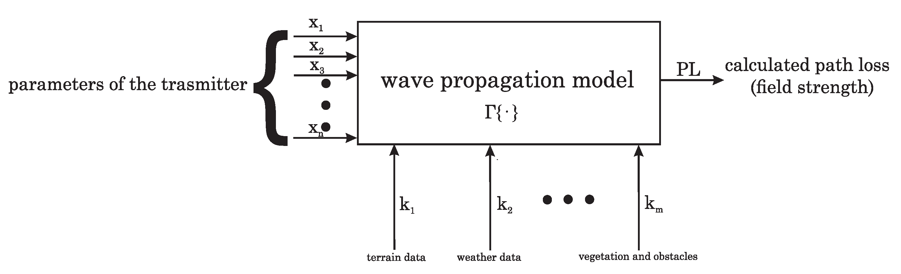
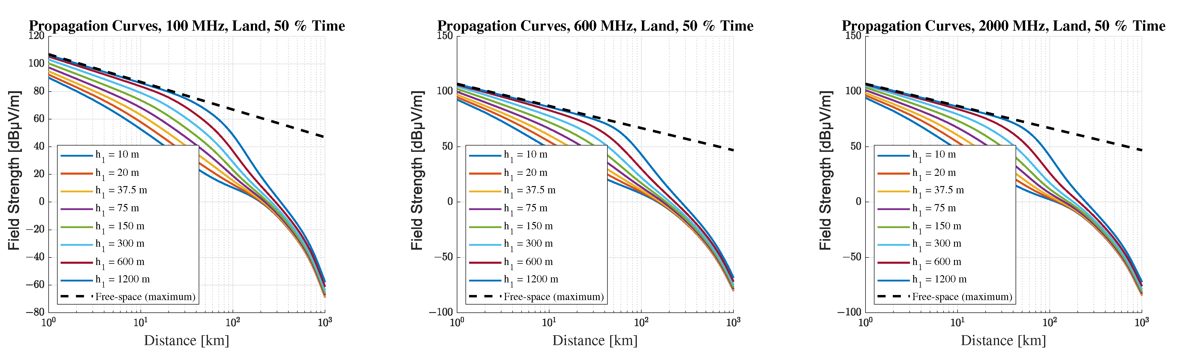
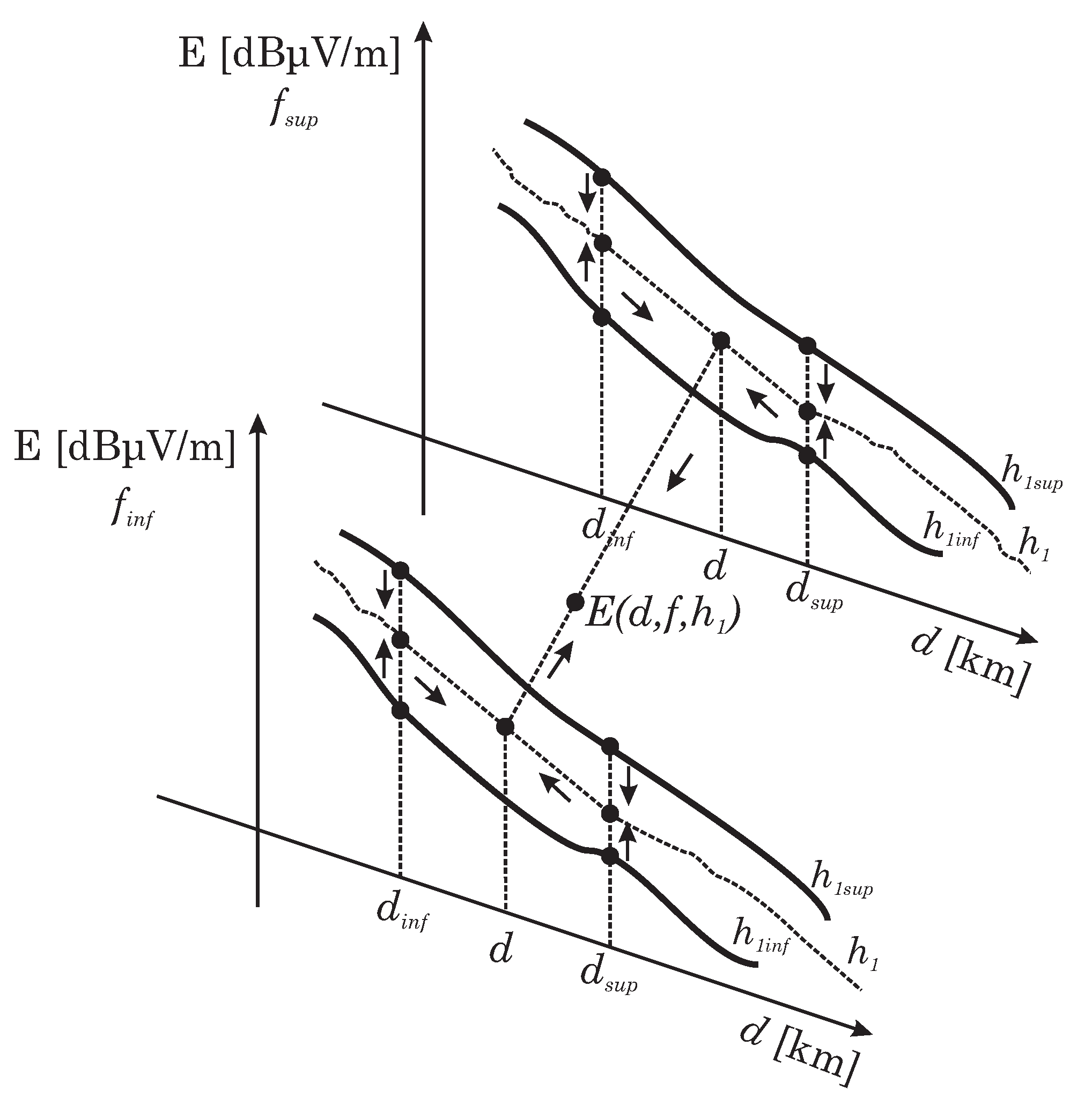
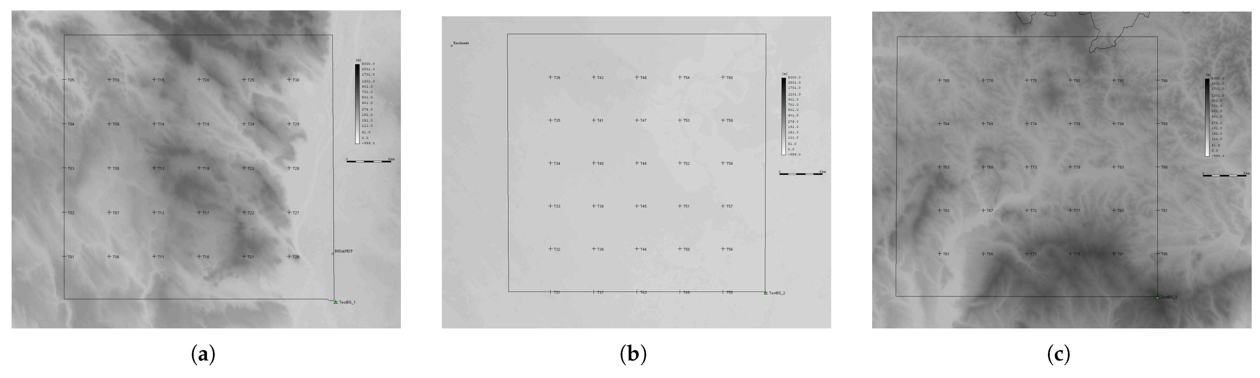
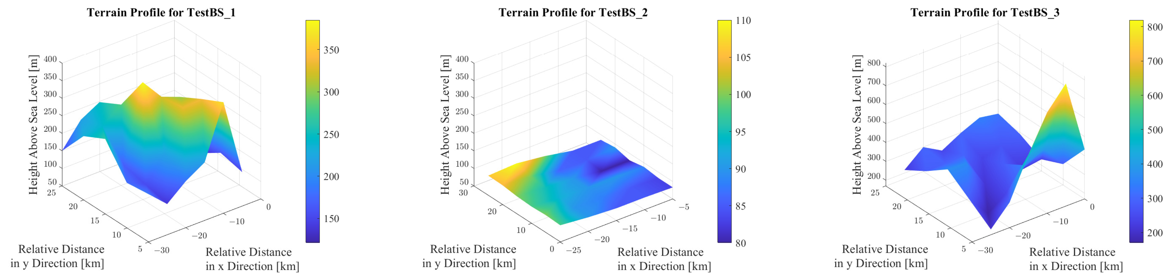
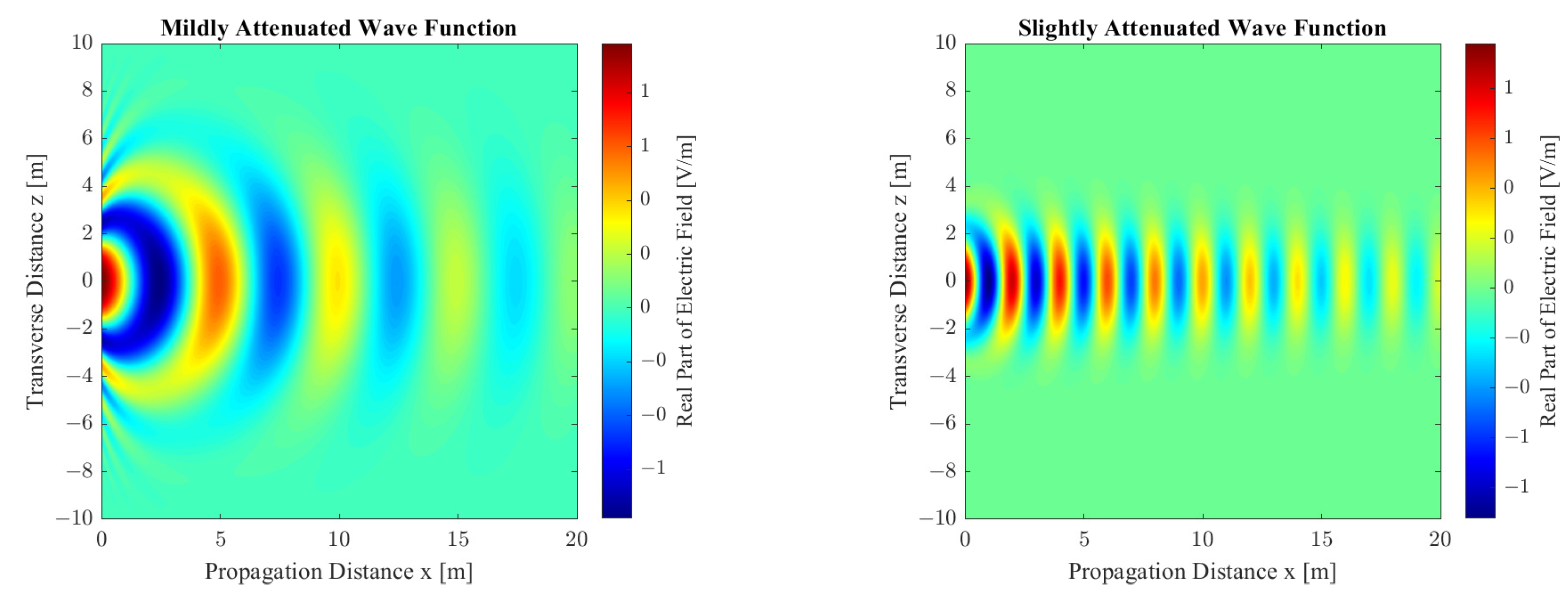
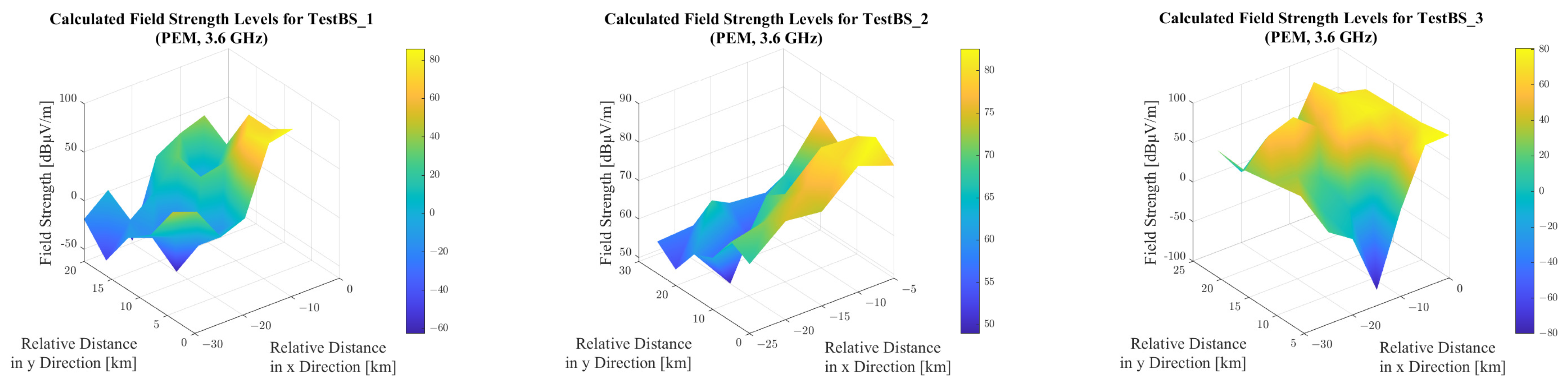
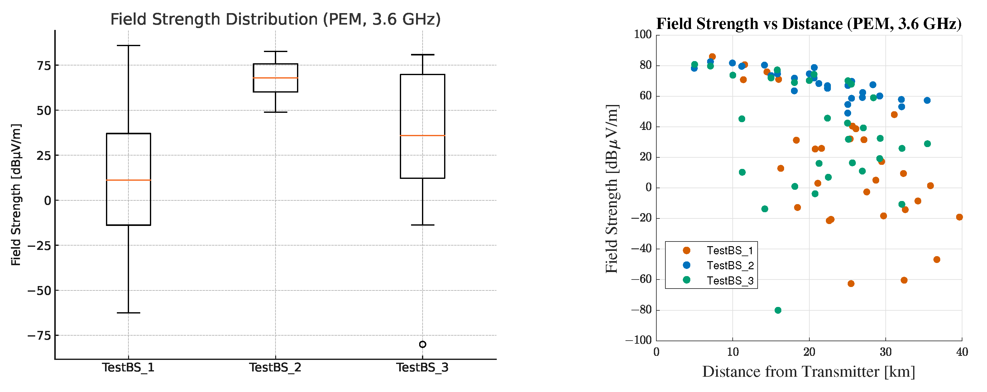
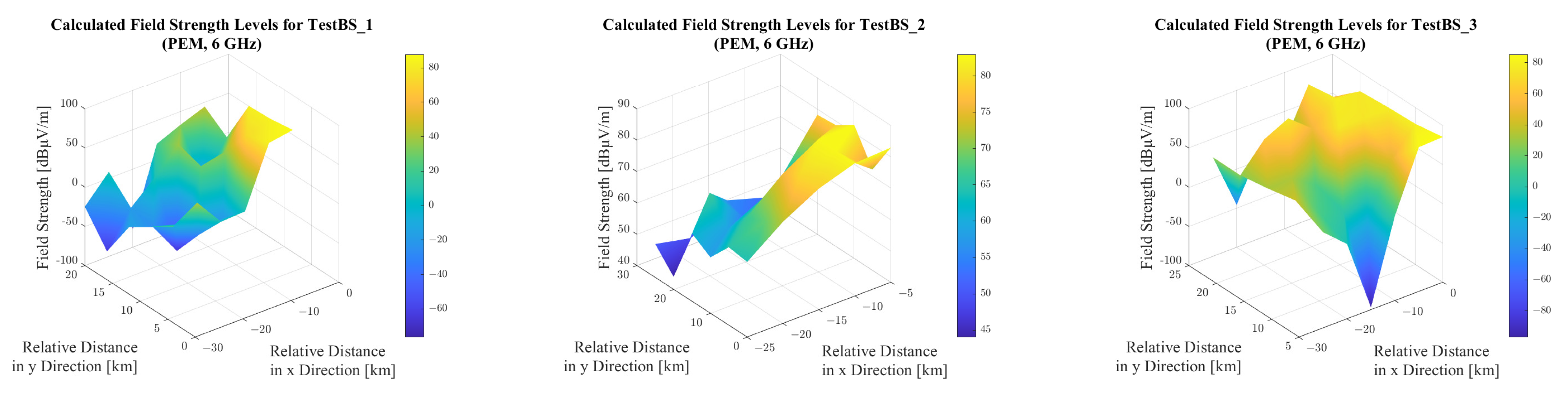
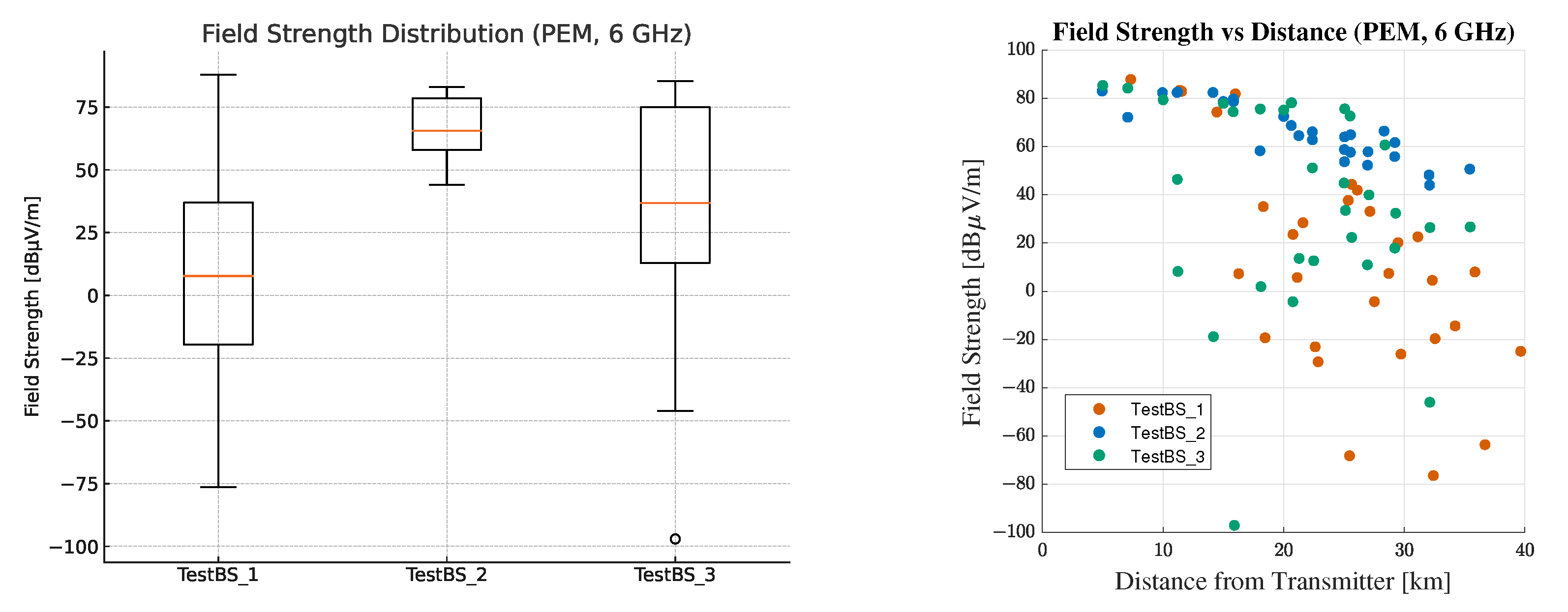
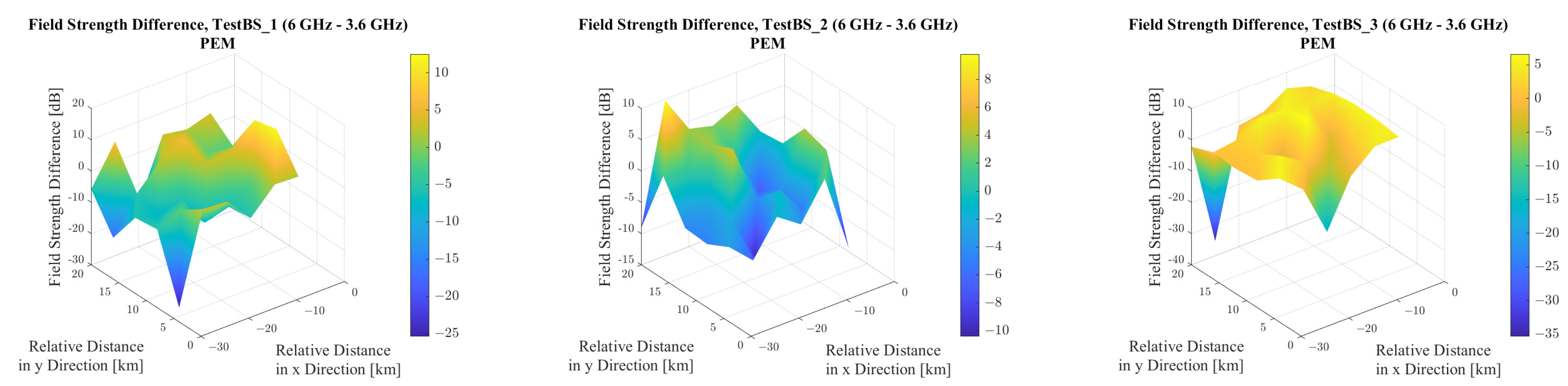
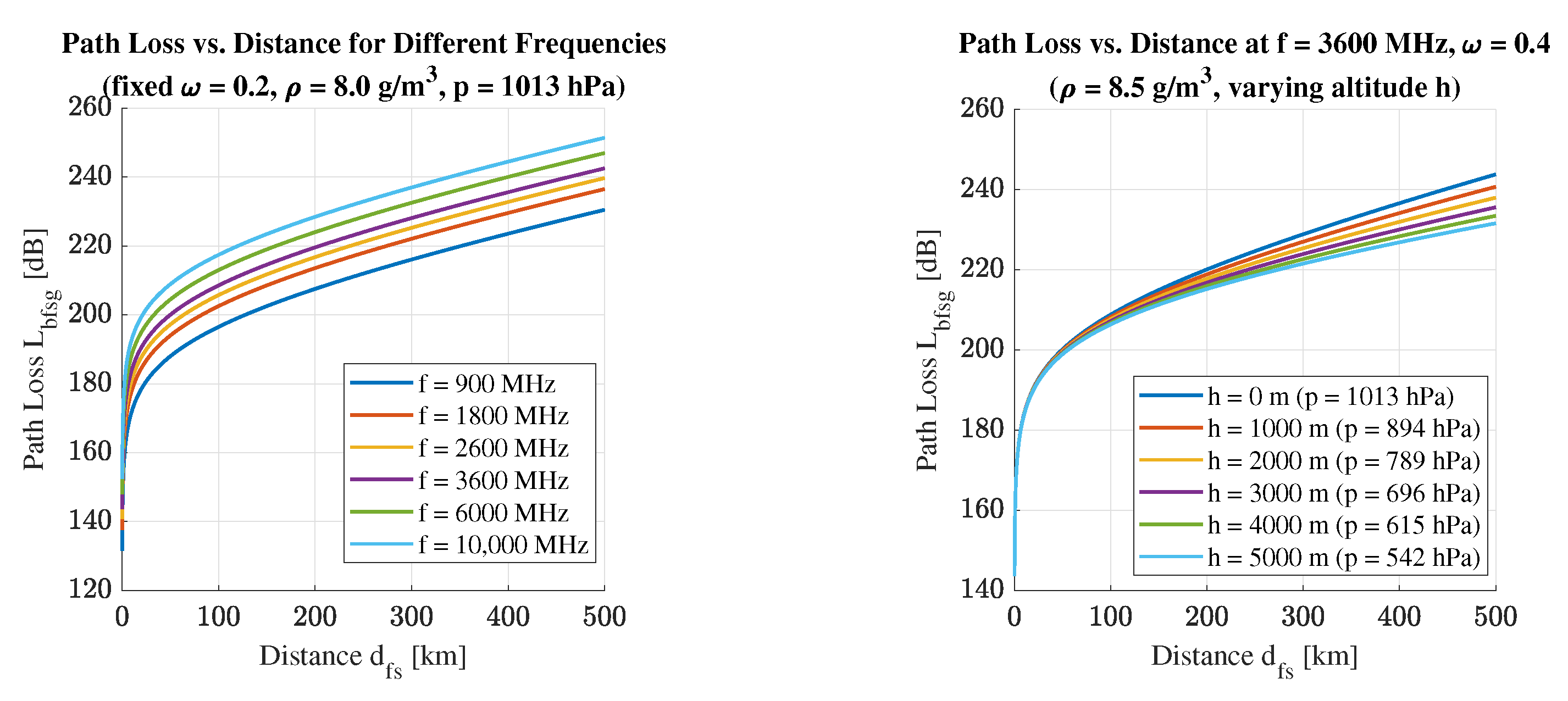
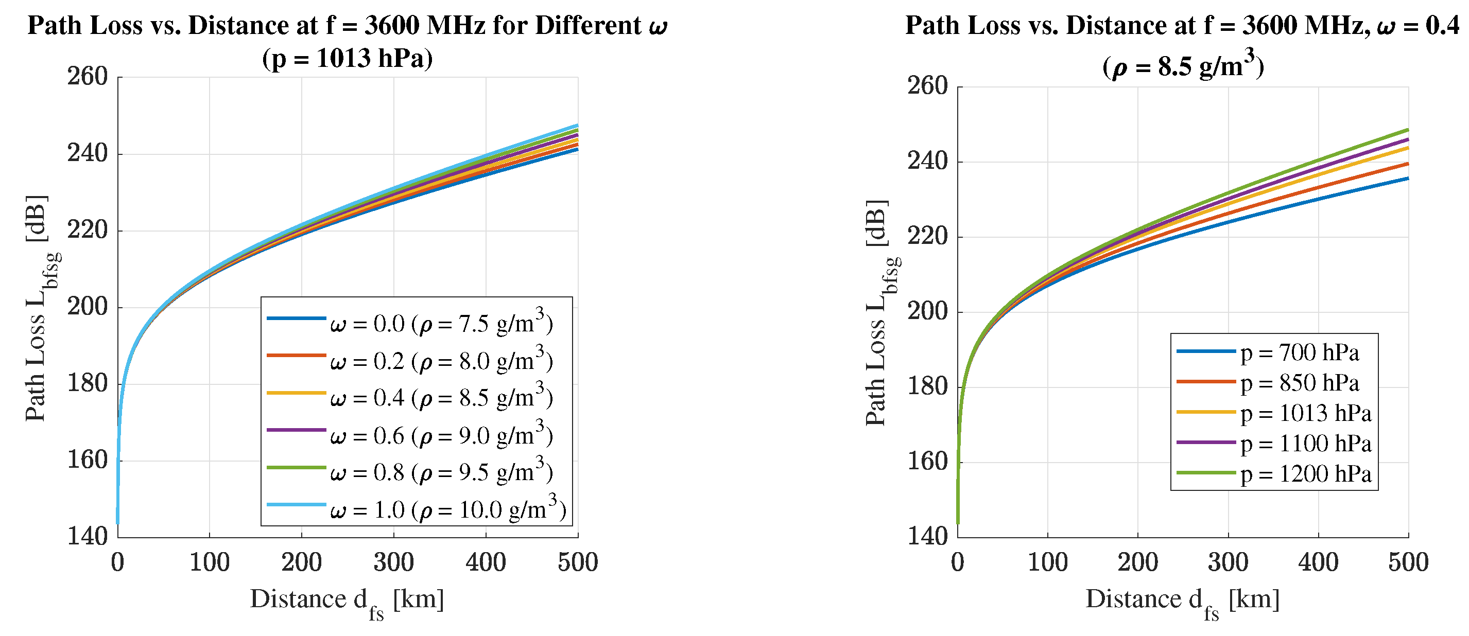
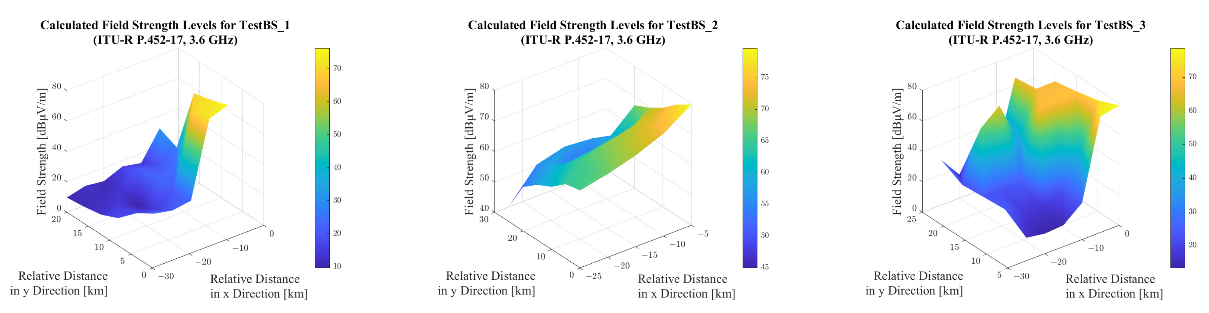
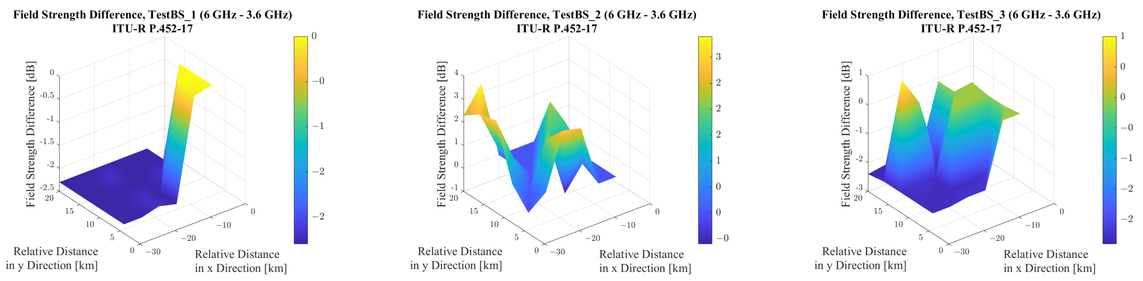
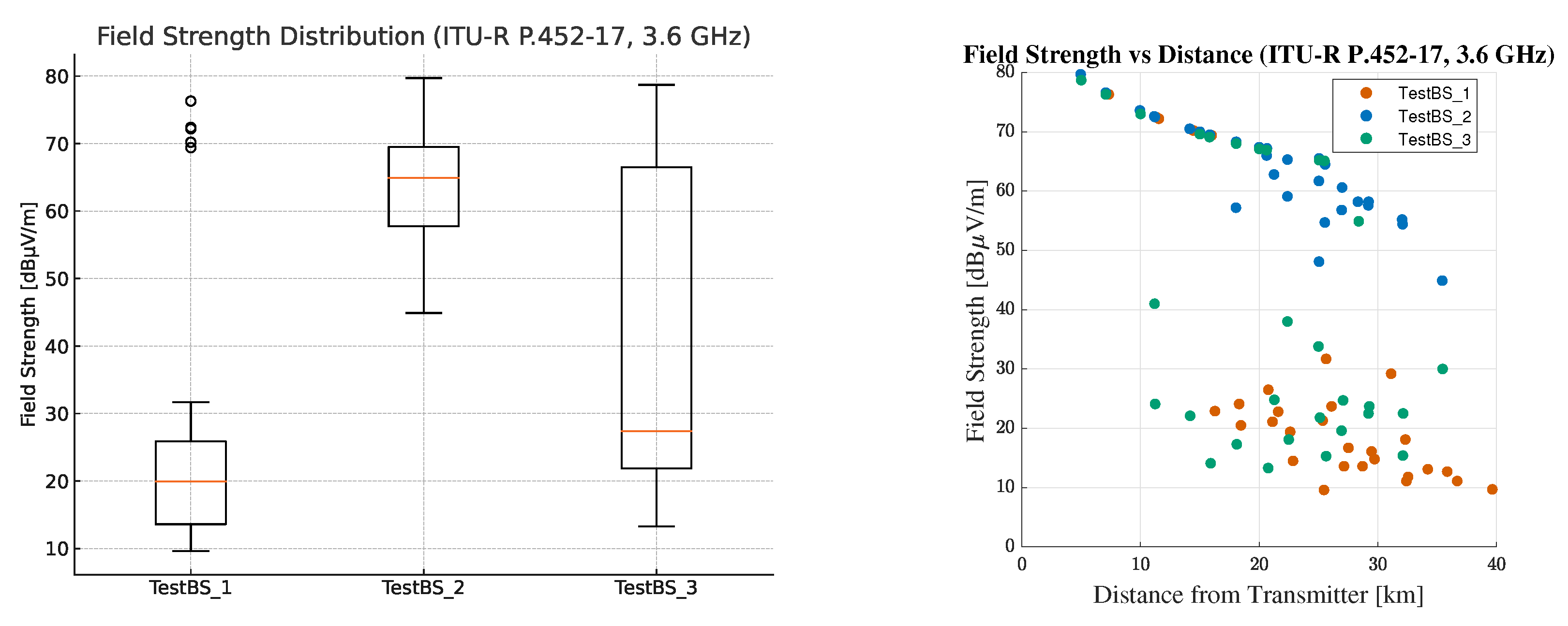
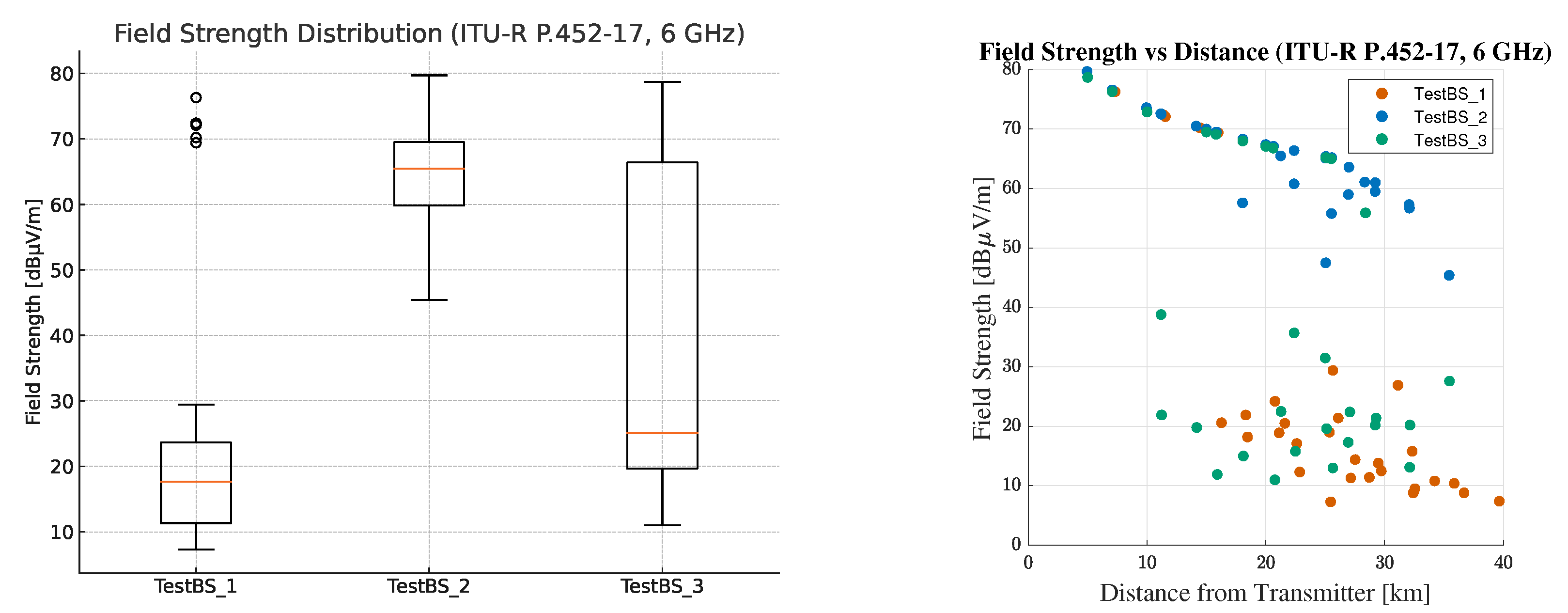
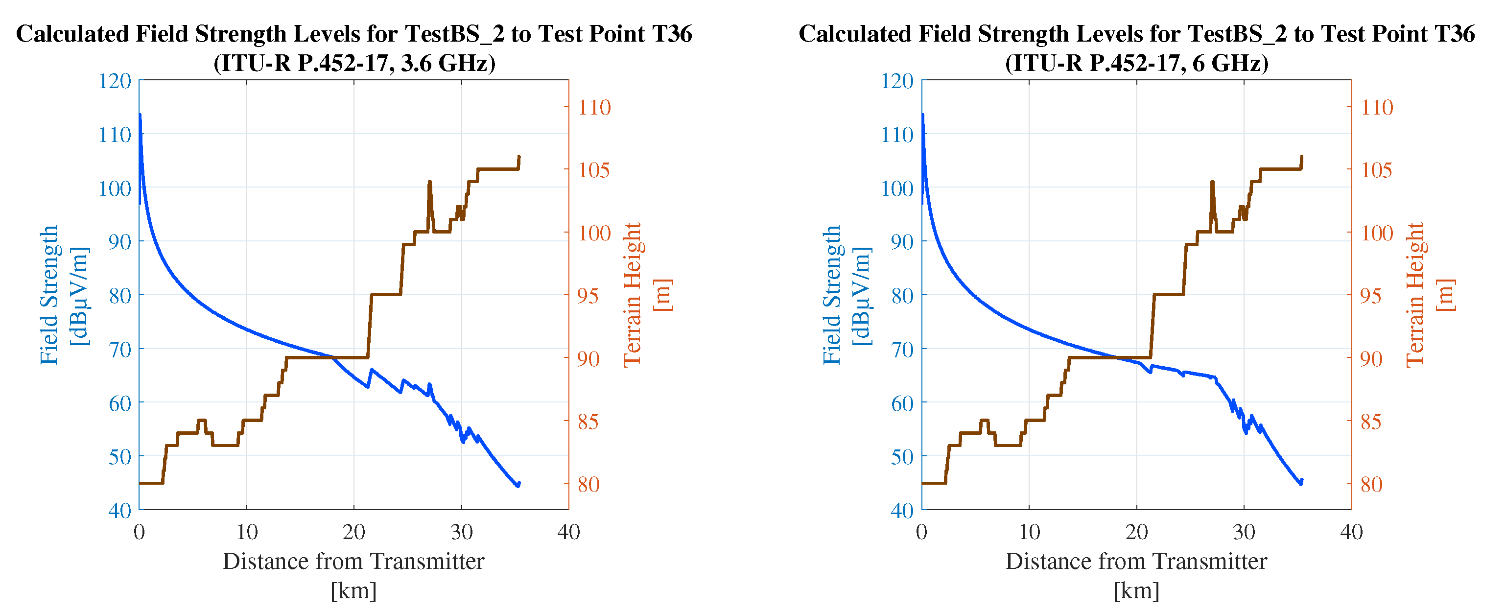
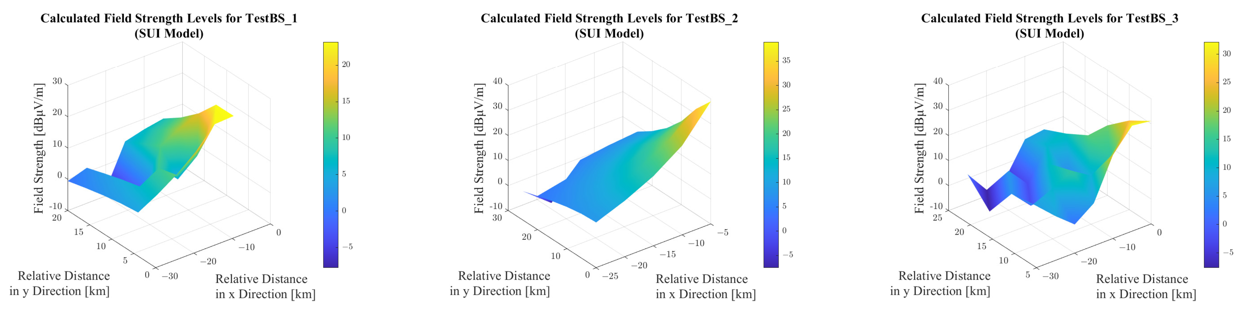
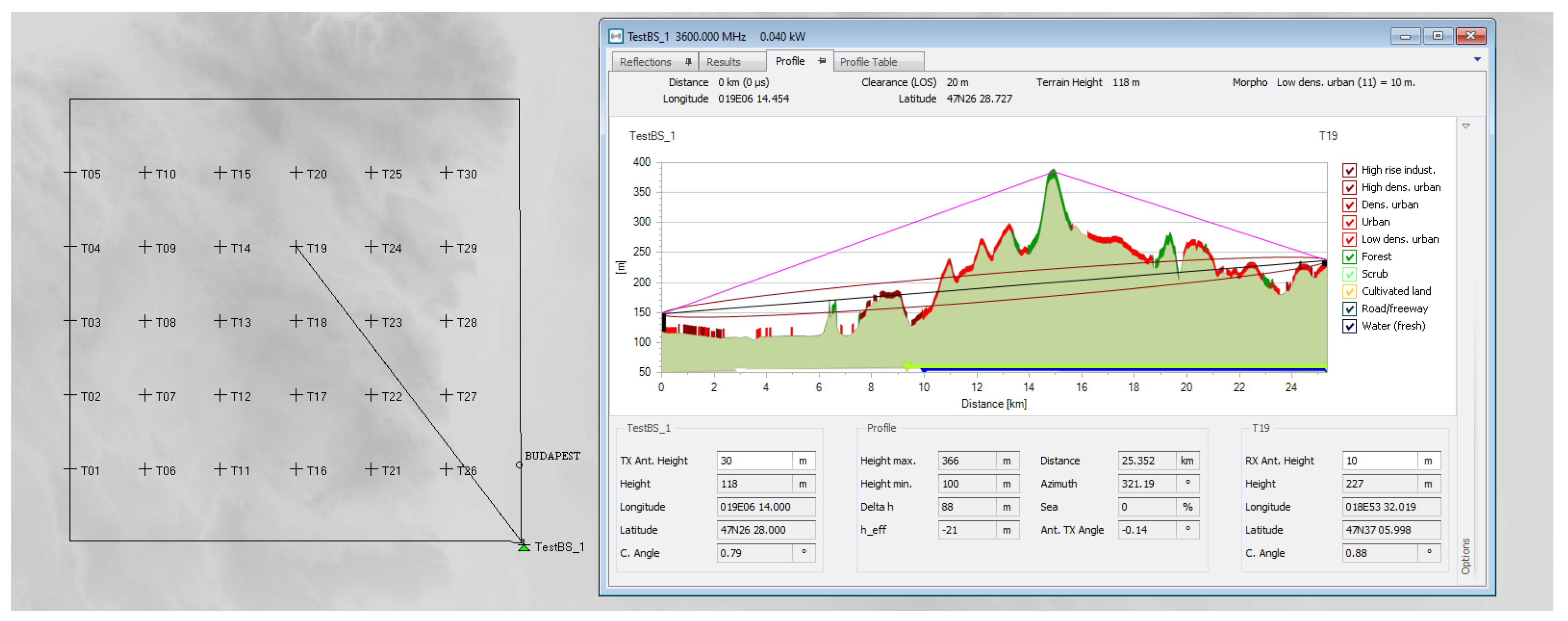
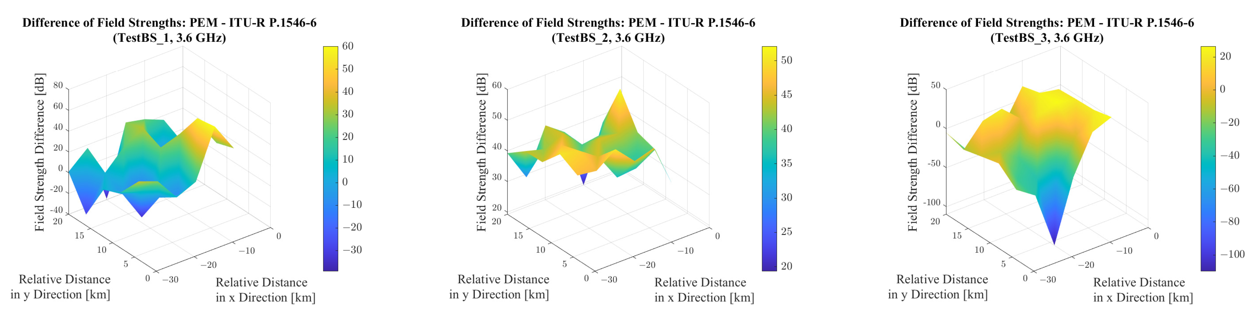
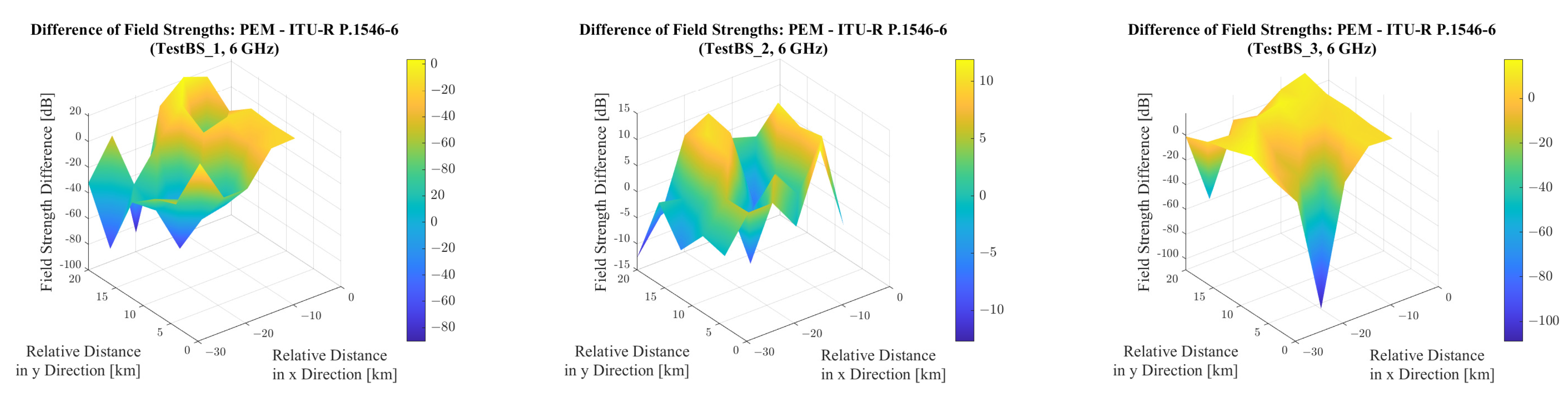
Table 16. Summary of model characteristics based on terrain sensitivity, bias direction, and relative error.

Model	Terrain Sensitivity (r)	Relative Error	Bias Direction	Reliability	Recommended Use
PEM	high ($r>0.8$)	reference (0%)	neutral	excellent	reference model, AI training, validation
ITU-R P.1546-6	low or negative	very high (40–630%)	underestimation	weak	flat terrain, large-scale estimates
SUI	low ($r<0.4$)	high (65–220%)	underestimation	weak	fast, low-complexity estimation
ITU-R P.452-17	high ($r>0.9$)	low (8–72%)	mild overestimation	good–excellent	spectrum planning, terrain-aware modeling

.