Optimal Partitioning of Unbalanced Datasets for BGP Anomaly Detection

Abstract

The Internet plays a vital role in the exchange of information in society. Maintaining the security and robustness of the Internet anomaly detection in Border Gateway Protocol (BGP) traffic is very important so that stable routing services can be ensured. The existing solutions are based on the classical machine learning (ML) models, which need to be advanced. In this study, a revolutionary technique that utilizes the Extreme Learning Machine (ELM) to enhance the detection of anomalies in the dynamic environment of the Border Gateway Protocol (BGP), particularly when faced with highly imbalanced class distributions, was used. The combination of imbalanced class distribution and BGP’s dynamic nature often leads to the suboptimal performance of classifiers. Our proposed solution aims to address this imbalance issue by dividing the dominant classes into multiple sub-classes. This division is achieved through optimal partitioning (OP), which involves segmenting the samples from the majority class into different segments to approximate the size of the minority class. As a result, diversified classes are created to train the ELM classifier. In order to assess the effectiveness of the proposed (OP-ELM) model, the RIPE and BCNET datasets were utilized. These trace files were processed using MATLAB to extract and organize the necessary features, thereby generating suitable datasets for analysis, which are referred to as Dataset-1 and Dataset-2. The experimental findings exhibit noteworthy improvements in performance when contrasted with prior methodologies, thereby highlighting the efficacy of our innovative approach in tackling the obstacles associated with anomaly detection in BGP networks.

1. Introduction

In the world of now very fast changing and dynamic computer networks, the Border Gateway Protocol (BGP) is a key protocol which helps in the routing of worldwide Internet traffic [1]. Nevertheless, the loose architecture and the BGP protocol design create the vision of BGP networks as vulnerable to the mixture of security anomalies, including route hijacks, prefix leaks, and DDoS attacks [2]. The continuous monitoring of these anomalies and eliminating them are absolutely essential to ensure the network stability, security, and integrity [3,4,5]. The ability to confront unbalanced datasets, with anomalous events making up an extremely small proportion of the total routing updates [5,6], is another critical challenge for BGP anomaly detection. Several different methods are used to detect BGP anomalies, as shown in [6,7,8]. However, the current methods for anomaly detection are based on using disproportionately imbalanced traffic data, an issue that cannot be overlooked. Furthermore, these techniques do not account for the changing conditions of networks’ environments. The result is inconsistency in data classification and data from time to time, adversely affecting the effectiveness of anomaly detection systems [9]. The methodology that proposes to tackle this issue should be capable of not only effectively learning from such imbalanced databases but also of adapting to the network dynamics by keeping a sufficient gap between the examples and the classifier decision boundaries.

The present article proposes a classification method based on the optimal partitioning (OP) and Extreme Learning Machine (ELM) [10] techniques for the identification of BGP anomalies with improved performance. The proposed method provides a practical solution to dataset imbalance by splitting classes with greater numbers of samples into several segments of smaller-sized subgroups and thereby making the distribution of samples even across the dataset. This segmentation is achieved through the use of OP, which facilitates classifying the samples from large classes into disconnected clusters, each of which is similar in size to the class with fewer samples. This approach leads to a more even distribution of the detection of anomalies inside BGP networks. The original concept for dividing samples from majority sample classes is taken from [11]; however, in this work, we extended the concept by applying the partitioning to multiple classes with higher numbers of samples. Furthermore, instead of using affinity propagation (AP) for partitioning the samples in this work, the optimal partitioning (OP) method based on Gray Wolf Optimization (GWO) [12] was utilized. Through this approach, classes with larger samples (major classes) are split into multiple clusters, and the clusters are assigned unique class IDs, which essentially makes them distinct sub-classes. These sub-classes together with the original classes with small numbers of samples (minor classes) are used for the Extreme Learning Machine (ELM) training. Figure 1 reveals the technique of deriving sub-classes from the major classes and merging them with the minor classes for the purpose of training the ELM. Here, the first dataset is divided into five classes, $D_1$ up to $D_5$, whose sample counts are $S_1$, $S_2$, $S_3$, $S_4$, and $S_5$, respectively. The unequal proportions of samples are illustrated by relatively more samples in $D_1$, $D_3$, and $D_5$ compared to in $D_2$ and $D_4$, which separately have fewer sample counts. For achieving uniform distribution, the method starts off by computing the mean number of samples per class, which is represented by the following equation:

$$S_M={\displaystyle \frac{{\sum }_{i=1}^5{S}_i}{5}}$$

(1)

Utilizing the mean sample size per class ($S_M$) as a standard comparator, the majority classes with sample counts higher than $S_M$ are divided into a number of sub-classes through optimal partitioning (OP). This implies that the distribution of the samples for the unbalanced classes will be brought back to its level in the former dataset because now the dataset has over five classes. The advantage of subdividing the larger sample size classes is also illustrated in Figure 2. It is important to note that these sub-classes serve a temporary role in the classification process. They are merged back to the initial classes of the classifier before the last phase of outputting. The outcome labels of the classifier are the original input labels.

The claimed contributions of this article are as follows:

• A novel classification method is proposed that uses optimal partitioning (OP) and the Extreme Learning Machine (ELM) for the classification and detection of anomalies in the traffic of BGP-based network environments;
• To handle the data imbalance nature of the dataset, the majority classes are targeted for optimal partitioning using the Particle Swarm Optimization technique;
• In the experiment, the Random Forest (RF), Support Vactor Machine (SVM), Artificial Neural Network (ANN), and Extreme Learning Machine (ELM) were trained and tested on the BGP traffic dataset, namely, BGP RIPE and BGP ROUTE Views;
• The results of the trained models were compared mutually, and it was determined that the OP-based ELM model provided the best results when different performance metrics were observed and experimentation was performed w.r.t. the accuracy, precision, recall, and F1-score, which acted as the proposed model to identify anomalies in BGP traffic;
• A comparison of the proposed model was also conducted with other recent state-of-the-art model approaches, and it was found to be the superior performing model.

The remaining organization of this article is as follows: Section 2 expresses the summary of related works as a Literature Review for BGP anomaly detection. Section 3 presents the proposed approach. Section 4 highlights the performance evaluation metrics, and in Section 5, the analysis of the results of the designed method are presented. Section 6 presents the conclusion of the paper for anomaly detection.

2. Literature Review

There have been different methodologies explored by examining the stances of traffic for network anomaly detection. The most generic way is to evolve the handling of the traffic behavior by the usage of statistical-based approaches. This leads to the identification of anomalies as they are highly correlated, and in the case of any abrupt change that happens in major segmentation, is also helpful in their recognition [13,14,15]. The disadvantage of the mentioned cases is that it is complicated to calculate the dimensional distributions. In order to recognize the anomalies from all of the data points present in the traffic, several clustering techniques have also been articulated. The anomalous data points that pertain to a single cluster and the anomalous data points that pertain to multiple clusters are recognized from all of the data points [16,17,18]. Clustering methodologies come with common downsides, such as automatic cluster description generation, random starting phase sensitivity, the presence of noise and outliers, the inability to process non-convex clusters of different sizes and densities, the vaguely defined completion criteria, and the overly complicated computations for high-dimensional datasets and big data. Therefore, there is the possibility of performance deterioration in higher-dimensional space [19]. In the traditional data mining domain, the approach is based on the ruling technique [20,21], which classifies members on the basis of a predefined set of rules and is another popular method. But its ability to detect anomalies through predefined rules is limited, and it is unable to detect unknown anomalies. Moreover, it demands a higher level of database scans to create the rules [22]. Several machine learning methodologies have also been adopted to complete this task. The completion of this task is achieved by separating it into two main parts: the first one is the unsupervised machine learning technique and the second one is the supervised machine learning technique [7]. One technique for the efficient detection of anomalies in the machine learning process is Artificial Neural Networks (ANNs) [23,24,25]. The strong point of neural networks is that they can detect the intricate kind of relationship between features; however, they also have many drawbacks, such as the substantial amount of data required for effective training. The training is computationally intensive and may take considerable time. The black-box nature of ANNs, which encompasses the capacity to infer how a particular decision or prediction is reached, is another feature. Additionally, ANNs are easily susceptible to overfitting, and this is a problem when the network architecture is much more complex in relation to the number of training data. As a result, the networks show poor generalization when handling new data that the networks have not encountered during the training process [26]. One of the primary SVM advantages that eliminates some of the ANN shortcomings is its ability to work with non-linear data [27]. SVMs apply the methodology of kernel functions to map the data points in the hyperplane. This is performed by the advent of a linearly distinguishable optimal hyperplane. The searching of the optimal hyperplane is performed, which distinguishes the data points linearly from the mapping space [28,29,30]. Different varieties of SVM detection approaches have been explored, and an evaluation of their performances is presented in [31,32]. Besides their advantages, they also face computational problems that are complex and, hence, increase the computing time and cost. The second fact is that support vector machines are not good in training datasets with unclear class labels because they rely heavily on the correct identification of the location of the decision boundaries. On top of that, SVMs are required to have better comprehension for good kernel selection as well as parameter tuning (like the regularization parameter C changes and the changes in the kernel parameters), which can be challenging and time-consuming [31,33,34,35].

A growing and revolutionary technique in the machine learning field today that is considered an alternative to ANNs and SVMs is the Extreme Learning Machine (ELM). The ELM is a conventional fully connected-type feedforward network, with the initial implementation in 2006 [36]. A single-layer feedforward neural network with hidden states (SLFN) in the ELM is essentially fast and similar in accuracy to that of support vector machines (SVMs); however, compared to SVMs, their training is much simpler [37]. Extreme Learning Machines (ELMs) are outstanding compared to support vector machines (SVMs) and Artificial Neural Networks (ANN) due to the speed and effectiveness of the entire training process [36]. ELMs eliminate the retraining of SVMs and ANNs required in iterative operations and are thus dramatically faster. Instead of the heavy reliance on the complex tuning of the SVM parameters and the extensive hyperparameter tuning of ANNs [37,38], ELMs bypass this troublesome process. While ELMs may be black boxes sometimes and might not always be perfect for all accuracies, their speed, simplicity, and ability to handle big datasets count as their key features and make ELMs an excellent option for multiple machine learning applications.

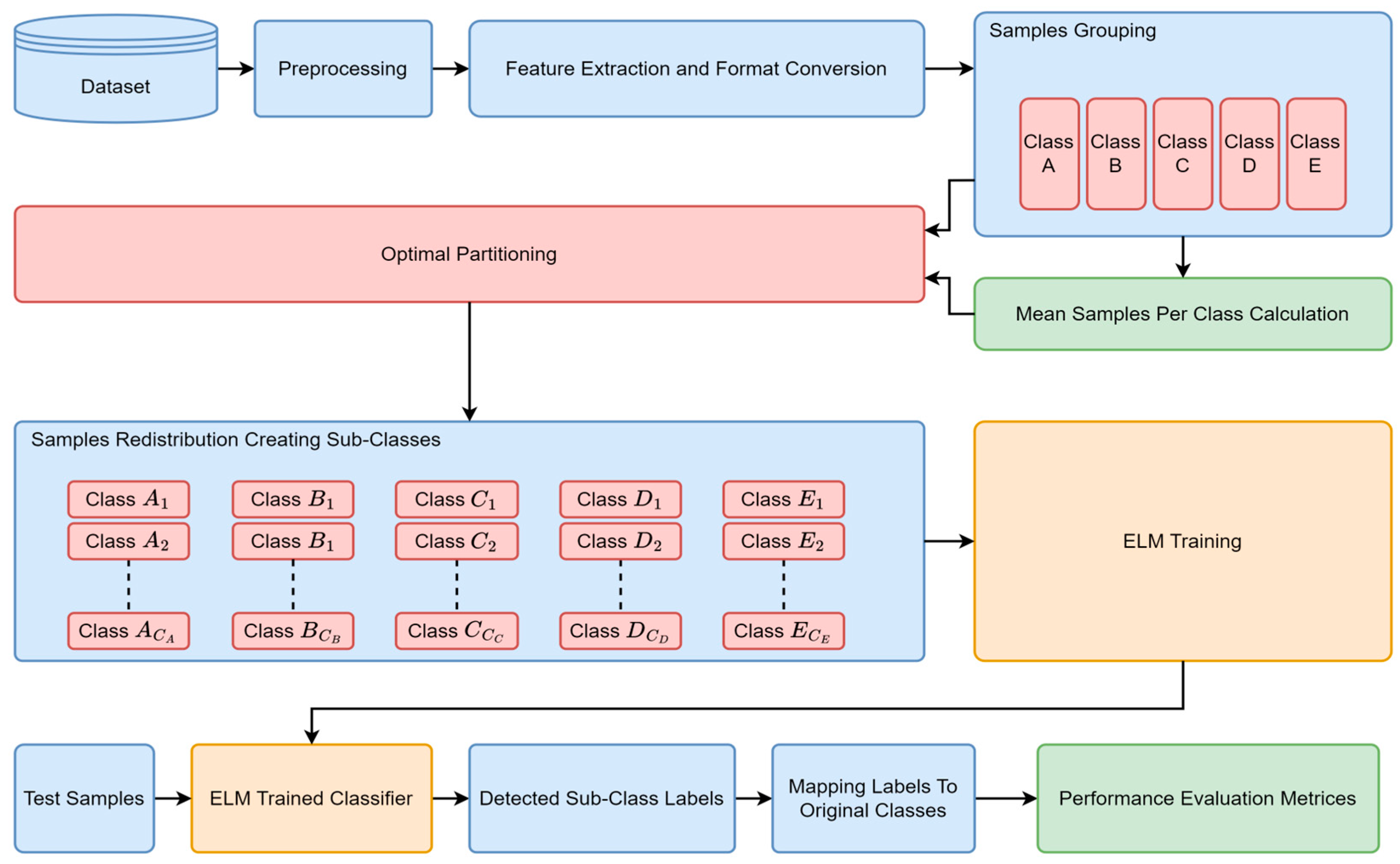
3. Proposed Approach

The present section is focused on the illustrative implementation and presentation of optimal partitioning and the Extreme Learning Machine (ELM). The algorithm based on the clustering technique that is mostly used in unsupervised learning is optimal partitioning, generally utilized in machine learning, while the ELM is a single-hidden-layer feedforward neural network (SLFN), which is fast for the training of the data, and the accuracy is comparatively similar to that of SVMs [36].

3.1. Optimal Partitioning (OP)

Dataset partitioning is a challenging task; it consists of dividing a given dataset into multiple subsets while preserving the key attributes of the original dataset in each subset. This work is a fundamental part of different data analysis processes, such as grouping, assigning, and anomaly recognition. We applied this idea to balance the dataset by separating the samples from the dominant classes into multiple sub-class clusters. The process virtually increases the number of classes but makes the class distribution even. To achieve this, in the presented work, we propose the optimal partitioning scheme, which utilizes the Gray Wolf Optimization (GWO) [12] algorithm to optimally partition the data samples from the majority classes. The GWO algorithm, modeled after how gray wolves hunt and coordinate, has become a favorite optimization scheme, as it had been shown in several optimization domains to be a very powerful tool. The capability of imitating the leadership order found among wolves as well the cooperation shared among the pack members make it a sensible candidate for optimizing complex problems. This synergy between GWO and dataset partitioning is explored in the proposals. Its aim is to develop an algorithm that is efficient at processing imbalanced datasets. The goal is to assign data instances from the majority classes to partitions (clusters) in such a way that class imbalance reduction, better classification accuracy, and class distribution balance are provided. The class evenness of each partition is kept as well. In the proposed methodology, the GWO algorithm is tuned to detect the best partitioning criterion as far as the imbalanced dataset is concerned. The GWO algorithm’s search mechanism performs this to determine the best partitioning scheme that seeks to maximize the inter-cluster separability and minimize the intra-cluster variance. With this, it is ensured that every subset created during the partitioning step keeps the ratio of the various classes present in the balanced dataset. To achieve this, the GWO algorithm is customized to treat the problem of dataset partitioning as a multi-objective optimization task. The algorithm iteratively adjusts the boundaries of each data subset based on the fitness function, which quantifies the quality of the partitioning. The fitness function considers factors such as the class distribution, data density, and intra-class similarity. The whole process can be explained as follows:

Objective: The Gray Wolf Optimization (GWO) algorithm optimizes the clustering with a given number of clusters ($N$), maximizing the inter-class separability and minimizing the intra-class variance. The GWO searches for the best positions of the centroids to achieve this goal;

Objective Function: The objective is to minimize the intra-class variance (within-cluster sum of squares ($WSS$)) while maximizing the inter-class separability (between-cluster sum of squares (BSS)). However, these goals are inherently balanced in a clustering context because minimizing the WSS typically leads to maximizing the BSS. Thus, our fitness function can primarily focus on minimizing the WSS, with the BSS being indirectly affected. We also need to adjust the fitness evaluation to penalize deviations from equal cluster sizes.

Considering the $WSS$, $BSS$, and penalty for unequal cluster sizes, the representation of the objective function is as follows:

$$F={\displaystyle \frac{BSS}{WSS+\lambda \times P}}$$

(2)

where $\lambda$ is a regularization parameter which is used for controlling the impact of the cluster size penalty ($P$). The goal is to maximize the $F$, thus minimizing the $WSS$, maximizing the $BSS$, and enforcing cluster size balance. Also, the $WSS$, $BSS$, and $P$ are calculated as follows:

$$WSS=\sum _{k=1}^N\sum _{x\in C_k}{‖x-{\mu }_k‖}^2$$

(3)

where $C_k$ is the set of points in cluster $k$, and ${\mu }_k$ is the centroid of cluster $k$;

$$BSS=\sum _{k=1}^N{n}_k{‖{\mu }_k-\mu ‖}^2$$

(4)

where $n_k$ is the number of points in cluster $k$, and $\mu$ is the overall mean of the data;

$$P=variance\left(\right\{n_1,n_2,\dots ,n_N\left\}\right)$$

(5)

where $n_k$ is the number of points in cluster $k$;

Algorithm Steps:

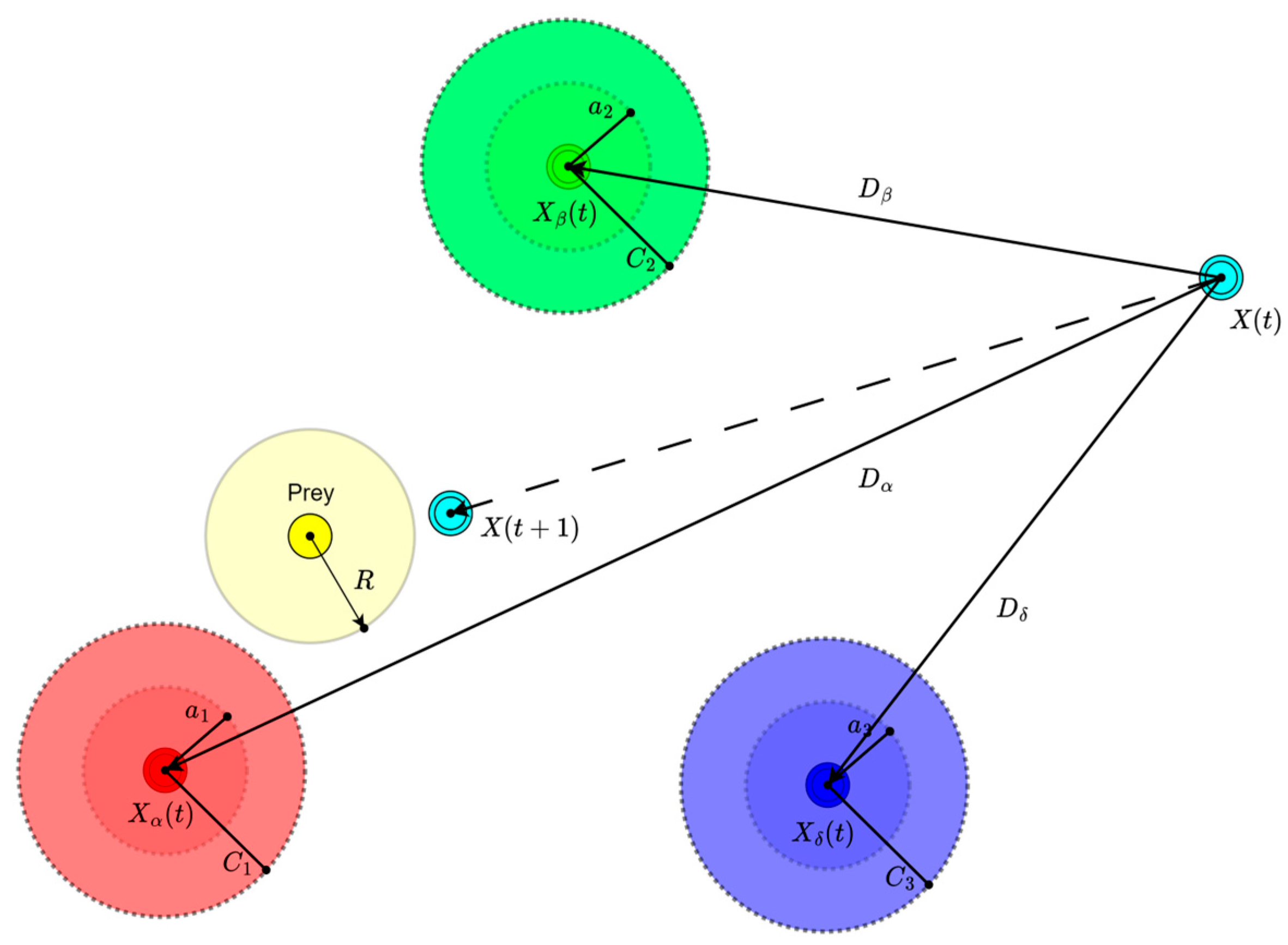
• Initialization: Generate an initial population of gray wolves (solutions). Each wolf’s position represents a potential set of centroids for the $N$ clusters.
• Fitness Evaluation: Calculate the fitness of each wolf using the Equation (2), the higher $F$ values indicate better solutions.
• Update Alpha ($\alpha$), Beta ($\beta$), and Delta ($\delta$) Wolves: Identify the best three solutions based on their fitness, assigning them as the $\alpha$, $\beta$, and $\delta$ wolves, representing the best ($X_{\alpha }$), second-best ($X_{\beta }$), and third-best ($X_{\delta }$) solutions, respectively and are demonstrated in Figure 3.
• Hunting (Main Optimization Loop)

The wolves update their positions towards the prey (optimal solution), influenced by the positions of the $\alpha$, $\beta$, and $\delta$ wolves that are presented in Figure 3.

The position update can be represented as follows, where $t$ is the current iteration:

$$\begin{gathered} {\overrightarrow{D}}_{\alpha }=\left|{\overrightarrow{C}}_1\cdot {\overrightarrow{X}}_{\alpha }\left(t\right)-\overrightarrow{X}\left(t\right)\right| \\ {\overrightarrow{D}}_{\beta }=\left|{\overrightarrow{C}}_2\cdot {\overrightarrow{X}}_{\beta }\left(t\right)-\overrightarrow{X}\left(t\right)\right| \\ {\overrightarrow{D}}_{\delta }=\left|{\overrightarrow{C}}_3\cdot {\overrightarrow{X}}_{\delta }\left(t\right)-\overrightarrow{X}\left(t\right)\right| \end{gathered}$$

(6)

$$\begin{gathered} {\overrightarrow{X}}_1={\overrightarrow{X}}_{\alpha }\left(t\right)-{\overrightarrow{A}}_1\cdot {\overrightarrow{D}}_{\alpha } \\ {\overrightarrow{X}}_2={\overrightarrow{X}}_{\beta }\left(t\right)-{\overrightarrow{A}}_2\cdot {\overrightarrow{D}}_{\beta } \\ {\overrightarrow{X}}_3={\overrightarrow{X}}_{\delta }\left(t\right)-{\overrightarrow{A}}_3\cdot {\overrightarrow{D}}_{\delta } \end{gathered}$$

(7)

$$\overrightarrow{X}(t+1)={\displaystyle \frac{{\overrightarrow{X}}_1+{\overrightarrow{X}}_2+{\overrightarrow{X}}_3}{3}}$$

(8)

where $X\left(t\right)$ denotes the position of the current wolf, while $X_{\alpha }\left(t\right)$, $X_{\beta }\left(t\right)$, and ${\overrightarrow{X}}_{\delta }\left(t\right)$ are the positions of the alpha, beta, and delta wolves (centroids of the best solutions), respectively. ${\overrightarrow{C}}_1$, ${\overrightarrow{C}}_2$, and ${\overrightarrow{C}}_3$ are the coefficient vectors for controlling the distance, and ${\overrightarrow{A}}_1$, ${\overrightarrow{A}}_2$, and ${\overrightarrow{A}}_3$ are the coefficient vectors for controlling the influence of the alpha, beta, and delta positions on the current wolf’s position. The coefficient vectors $A_i$ and $C_i$ are calculated as follows:

$$A_i=2a\cdot r_1-a$$

(9)

$$C_i=2\cdot r_2$$

(10)

where $\overrightarrow{a}$ linearly decreases from $2$ to $0$ over iterations, and ${\overrightarrow{r}}_1$ and ${\overrightarrow{r}}_2$ are random vectors in [0, 1].

• Termination: repeat the optimization loop until the stopping criterion is met (e.g., maximum iterations ($T$) or minimal change in fitness);
• Result: The final positions of the alpha wolf represent the centroids of the clusters that optimally partition the data according to the given $N$. The cluster assignments reflect the balance between minimizing the intra-class variance, maximizing the inter-class separability, and maintaining approximately equal cluster sizes, as influenced by the fitness function.

This approach, by dynamically updating the positions of the wolves towards the best solutions ($\alpha$, $\beta$, and $\delta$), simulates the collaborative hunting strategy of gray wolves. It allows for both the exploration of the search space (to avoid local minima) and the exploitation of the best-found solutions (to refine them), aiming to find an optimal clustering arrangement that minimizes the intra-cluster variance.

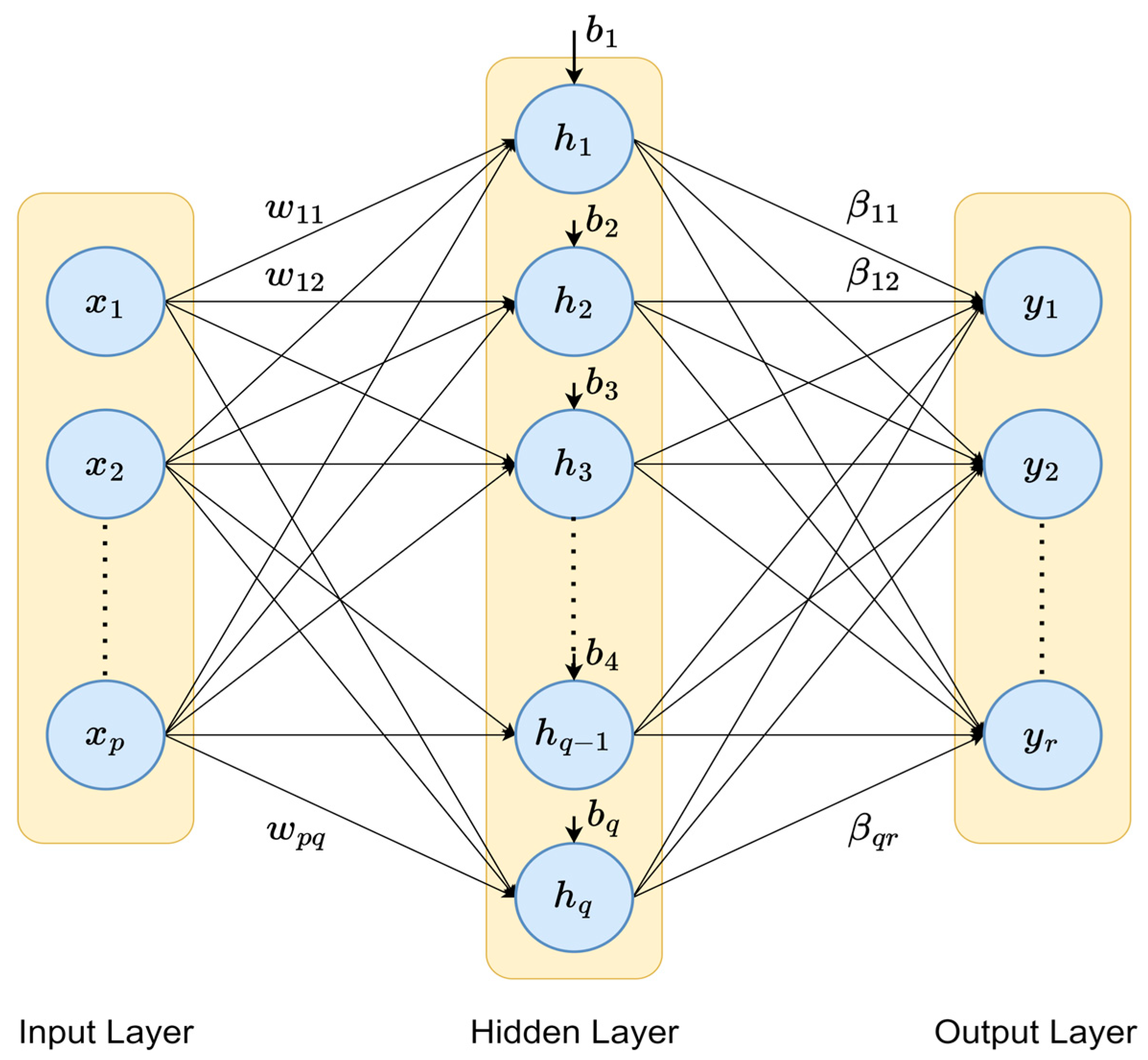
3.2. Extreme Learning Machine

The Extreme Learning Machine (ELM) is a single-layer feedforward neural network that consists of a single layer of hidden nodes [10]. It consists of weights which are randomly assigned among the input layer and the hidden layer, and which are not adjusted during training. Furthermore, the calculation of the weights associated with the output layer is performed by using a straight linear equation system that does not require iterations. This configuration grants fast training while maintaining an accuracy similar to that of other kernel-based machine learning systems [39].

3.3. ELM Functionality Explanation

This section explains the functionality of an ELM using the standard ELM architecture shown in Figure 4.

Input Layer: This layer consists of neurons that represent the input features. Each neuron corresponds to one feature of the data, denoted as $x_1$, $x_2$, $x_3$, …,$x_p$ features.

Hidden Layer: The hidden layer has a set of neurons, each with a random weight and bias connected to every input neuron. The weights are denoted by $w_{ij}$, where $i$ indexes the input neurons and $j$ indexes the hidden neurons. The biases are denoted as $b_1$, $b_2$, …, $b_q$ for $q$ hidden neurons. The output of the $j\mathrm{t}\mathrm{h}$ hidden neuron, denoted as $h_j$, is calculated using the activation function ($g$):

$$h_j=g\left(\sum _{i=1}^p{w}_{ij}{x}_i+b_j\right)$$

(11)

Here, $g\left(\cdot \right)$ is typically a non-linear function like the sigmoid, tanh, or ReLU [40].

Output Layer: The output layer neurons receive the output from the hidden layer neurons. The weights between the hidden layer and the output layer are denoted as ${\beta }_{ij}$, where $i$ indexes the hidden neurons and $j$ indexes the output neurons. The final output by the $j\mathrm{t}\mathrm{h}$ output neuron ($y_j$) is a linear combination of the hidden layer outputs:

$$y_j=\sum _{i=1}^q{\beta }_{ij}{h}_i$$

(12)

These weights ($\beta$) are determined by a linear system to minimize the error between the predicted outputs and the actual target values of the training data. The complete ELM system in matrix form can be given as follows:

$${\left[\begin{array}{c}{y}_1\\ y_2\\ ⋮\\ y_r\end{array}\right]}_{r\times 1}={\left[\begin{array}{cccc}{h}_1& h_2& \cdots & h_q\\ h_1& h_2& \cdots & h_q\\ ⋮& ⋮& \ddots & ⋮\\ h_1& h_2& \cdots & h_q\end{array}\right]}_{r\times q}\times {\left[\begin{array}{cccc}{\beta }_{11}& {\beta }_{12}& \cdots & {\beta }_{1r}\\ {\beta }_{21}& {\beta }_{22}& \cdots & {\beta }_{2r}\\ ⋮& ⋮& \ddots & ⋮\\ {\beta }_{q1}& {\beta }_{q2}& \cdots & {\beta }_{qr}\end{array}\right]}_{m\times r}$$

(13)

or

$$Y=H\times \mathrm{{\rm B}}$$

(14)

In an ELM, the key idea is that the weights and biases ($w$ and $b$) are set randomly and are not updated during training. Instead, only the output weights ($\beta$) are learned. This is achieved by solving the least-squares problem, typically using the Moore–Penrose pseudo-inverse:

$$\mathrm{{\rm B}}=H^{+}T$$

(15)

where $H^{+}$ denotes the pseudo-inverse [41] representation of the hidden layer output matrix ($H$), and $T$ is the target output matrix for the training data.

The ELM is efficient because it reduces the learning process to a single-step linear problem, bypassing the need for iterative optimization, such as the backpropagation used in traditional neural networks. This makes ELMs particularly fast for training while still allowing them to approximate complex functions given an adequately large number of hidden neurons.

3.4. Experimental Dataset Details

The raw data of the BGP were taken from the RIPE and BCNET collection sites. These datasets are collected under different anomaly conditions, as listed in

Table 1. BGP dataset details.

Dataset	Class	Date	Total Samples
Slammer	Anomaly	January 2003	7200
Nimda	Anomaly	September 2001	8609
Code Red I	Anomaly	July 2001	7200
WannaCrypt	Anomaly	May 2017	11,520
Moscow Blackout	Anomaly	May 2005	7200
Normal-BCNET	Regular	--	1440
Normal-RIPE	Regular	--	7196

.

The data which were collected from the traffic were filtered and distributed into various classes for listing the BGP anomalies shown in

Table 2. Class distribution details of dataset.

Anomaly Names	Class Labels	Dataset Class Instances
Normal	A	2000
Slammer	B	400
Nimda	C	200
Code Red I	D	600
WannaCrypt	E	1000
Moscow Blackout	F	1000

. It was observed that the MATLAB script produced higher numbers of events. However, in order to perform the experimentation, the finite number of events were selected in a random manner for every single class to obtain the imbalanced class distribution.

3.5. Feature Analysis

Since the information and characteristics influence the model’s classification output and define the upper limit of machine learning performance. The raw BGP data needs to be converted into a set of features with clear physical or statistical significance. To convert recorded trace data into the proper format and data type, MATLAB script was used, and 37 features were extracted from the given trace files.

Table 3. Feature definitions.

Feature	Definition	Type	Category
1	Number of announcements	Continuous	Volume
2	Number of withdrawals	Continuous	Volume
3	Number of announced NLRI prefixes	Continuous	Volume
4	Number of withdrawn NLRI prefixes	Continuous	Volume
5	Average AS-PATH length	Categorical	AS-path
6	Maximum AS-PATH length	Categorical	AS-path
7	Average unique AS-PATH length	Continuous	AS-path
8	Number of duplicate announcements	Continuous	Volume
9	Number of duplicate withdrawals	Continuous	Volume
10	Number of implicit withdrawals	Continuous	Volume
11	Average edit distance	Categorical	AS-path
12	Maximum edit distance	Categorical	AS-path
13	Inter-arrival time	Continuous	Volume
14–24	Maximum edit distance = $n$, where $n=(7, 8,\dots ,17)$	Binary	AS-path
25–33	Maximum AS_PATH length = $n$, where $n=(7, 8,\dots ,16)$	Binary	AS-path
34	Number of IGP packets	Continuous	Volume
35	Number of EGP packets	Continuous	Volume
36	Number of incomplete packets	Continuous	Volume
37	Packet size (B)	Continuous	Volume

shows the features obtained through the extraction process. These calculated feature values were normalized before using them for training and testing purposes. The normalization transformed the features into a common range that made all the features equally important irrespective of their numeric values [42].

3.6. Proposed Methodology

The proposed BGP anomaly detection model is shown in Figure 5.

The role in the classification is to make a category of testing labels into predefined classes, as presented in Table 1. Firstly, the BGP network traffic data are read from dataset files. These data files contain unprocessed original data obtained from the network. The processing of these originally obtained raw data is required so as to extract the desired information, as shown in Table 3. The implementation of the proposed methodology is featured by the utilization of MATLAB script to extract the desired information and transform it into specific data types. In order to make the operation of the mathematical computation in the desired manner, the data types are converted in a relevant manner, (such as by converting the character data type, categorical data, and ASCII to Integer, Float, and Double), as desired for the operation of connected blocks. As the problem of an imbalanced dataset is taken under consideration, where the occurrence of the events of Class A are five times more than the occurrence of other classes (shown in Table 1). Therefore, the events of Class $A$ are clustered into $C_A$ numbers of sub-classes (Class $A_1$ to Class $A_{C_A}$) using optimal partitioning. The number of clusters can be calculated by dividing the total samples by the mean samples per class. This leads to the transformation of the five-class imbalanced dataset into the $N=C_A+C_B+C_C+C_D+C_E$-class balanced dataset. Now, the balanced dataset presents $N$ classes, and it then undergoes processing through a feature selection block. This block selects the relevant features present in the dataset. The dataset, after being newly formed, is divided into five groups through the k-fold ($k=5$) cross-validation method. For evaluating the performance of the classifier, four out of the five groups are utilized for the training purpose of the ELM, whereas the rest of the group is reserved for testing. This process is performed repeatedly five times, ensuring that each group is uniquely selected for testing during each iteration, with the others used for training. The final outcome is determined by averaging the results of all five tests. To maintain balance, Class $A$ is initially divided into $C_A$ sub-classes, labeled as Class $A_1$ through Class $A_{C_A}$. Before the final evaluation, these sub-class labels are relabeled back to Class $A$. The relabeled results are then used to assess the final performance of the proposed system.

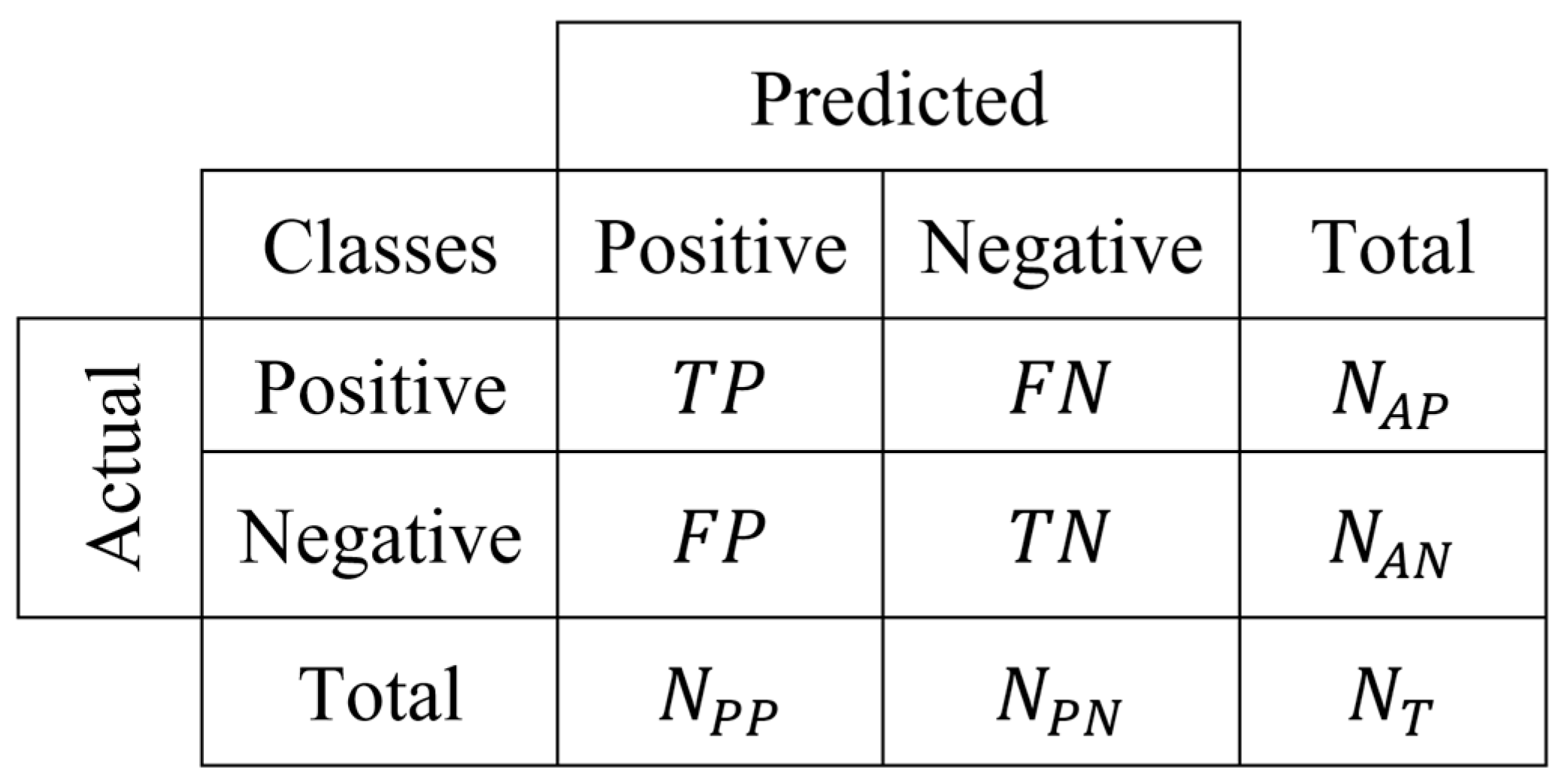
4. Performance Evaluation Metrics

The utilization of performance indicators is very helpful in analyzing the performance of any machine learning model. These indicators assist with comparing different classification approaches and machine learning techniques. The testing capability of different classifiers is observed on the basis of evaluation metrics. The confusion matrix is one of them and is responsible for the relevant information obtained from the algorithm. In Figure 6, a two-class confusion matrix is shown based on this matrix, and the four common measures are given as follows:

$$Accuracy={\displaystyle \frac{TP+TN}{TP+TN+FP+FN }}={\displaystyle \frac{TP+TN}{N_T}}$$

(16)

The accuracy in Equation (16) measures the proportion of correctly predicted instances (both true positives and true negatives) out of the total number of instances.

$$Precision={\displaystyle \frac{TP}{TP+FP }}$$

(17)

The precision in Equation (17) indicates the proportion of true positive predictions out of all instances predicted as positive.

$$Recall={\displaystyle \frac{TP}{TP+FN}}$$

(18)

The recall in Equation (18) measures the proportion of true positives out of all actual positive instances.

$$F=2·{\displaystyle \frac{Precision·Recall}{Precision+Recall}}$$

(19)

The F-measure in Equation (19) provides a harmonic mean of the precision and recall, offering a balance between the two metrics.

The terms $TP$, $TN$, $FP$, and $FN$ denote true positive, true negative, false positive, and false negative instances, respectively. Moreover, $N_{AP}$, $N_{AN}$, $N_{PP}$, and $N_{PN}$ represent the counts of actual positive instances, actual negative instances, predicted positive instances, and predicted negative instances, respectively. The term $N_T$ refers to the total number of instances within the test dataset.

These measurements can be extended for multiclass scenarios [43,44]. However, this first requires the expansion of the two-class confusion matrix into $M$ classes, as presented in Figure 7. In the figure, the term $N_{ij}$ denotes the number of $i\mathrm{th}$ class instances that are classified as $j\mathrm{th}$ class instances.

Using the confusion matrix shown in Figure 7, the different measures for multiclass classification can be given as follows:

The balanced accuracy adjusts for the class imbalance by considering the recall (true positive rate) of each class and averaging them. It is calculated as follows:

$$Ac{c}_{Bal}={\displaystyle \frac{1}{M}}\sum _{i=1}^M{\displaystyle \frac{N_{ii}}{N_i^A}}$$

(20)

The balanced precision is calculated by averaging the precision of each class. The balanced precision is the mean of the precision values for all classes, giving equal weight to each class regardless of its size:

$$Pr{e}_{Bal}={\displaystyle \frac{1}{M}}\sum _{i=1}^M{\displaystyle \frac{N_{ii}}{N_{ii}+{\sum }_{j=1,j\ne i}^M{N}_{ji}}}$$

(21)

The balanced recall (or balanced sensitivity) is the mean recall of all classes. For a class ($C_i$), the recall is defined as the ratio of true positives to the sum of true positives and false negatives for that class. The balanced recall is calculated as follows:

$$Re{c}_{Bal}={\displaystyle \frac{1}{M}}\sum _{i=1}^M{\displaystyle \frac{N_{ii}}{N_{ii}+{\sum }_{j=1,j\ne i}^M{N}_{ij}}}$$

(22)

The balanced F-measure is the harmonic mean of the balanced precision and balanced recall:

$$F_{Bal}=2·{\displaystyle \frac{Pr{e}_{Bal}·Re{c}_{Bal}}{Pr{e}_{Bal}+Re{c}_{Bal}}}$$

(23)

These measures can further extend to weighted balanced measures, which take into account the proportion of each class within the dataset. This is computed as the sum of the measures for each class, weighted by the proportion of actual instances in each class. Based on these considerations, the balanced accuracy weighted ($Ac{c}_{Bal+W}$), balanced precision weighted ($Pr{e}_{Bal+W}$), balanced recall weighted (Re$c_{Bal+W}$), and balanced F-measure weighted ($F_{Bal+W}$) are given as follows:

$$Ac{c}_{Bal+W}={\displaystyle \frac{1}{M}}\sum _{i=1}^M{\displaystyle \frac{N_{ii}}{N_i^A}}\times {\displaystyle \frac{N_i^A}{N_T}}$$

(24)

$$Pr{e}_{Bal+W}={\displaystyle \frac{1}{M}}\sum _{i=1}^M{\displaystyle \frac{N_{ii}}{N_{ii}+{\sum }_{j=1,j\ne i}^M{N}_{ji}}}\times {\displaystyle \frac{N_i^A}{N_T}}$$

(25)

$$R{ec}_{Bal+W}={\displaystyle \frac{1}{M}}\sum _{i=1}^M{\displaystyle \frac{N_{ii}}{N_{ii}+{\sum }_{j=1,j\ne i}^M{N}_{ji}}}\times {\displaystyle \frac{N_i^A}{N_T}}$$

(26)

$$F_{Bal+W}=2·{\displaystyle \frac{Pr{e}_{Bal+W}·Re{c}_{Bal+W}}{Pr{e}_{Bal+W}+Re{c}_{Bal+W}}}$$

(27)

5. Results Analysis

This section provides an in-depth analysis of the performance of the proposed OP-ELM model in BGP anomaly detection, as well as its ability to overcome class imbalance issues and detect BGP anomalies under different network conditions. We conducted extensive experiments on the RIPE and BCNET datasets and evaluated the model systematically with four different techniques—the Random Forest, SVM, ANN, and weighted ELM—and two variants incorporating oversampling and undersampling through the SMOTE and Tomek Link sampling techniques and some state-of-the-art baseline methods under various metrics, including the accuracy, precision, recall, and F1-score. The analysis investigated differences in the performance related to the majority and minority classes, investigated the impact of the balanced vs. weighted measurement approaches, and tracked the computational efficiency of the solution. These results not only validate the model’s technical contributions but also shed light on its practical applicability for real-world BGP security problems, which is critical where the detection accuracy and operational efficiency are prime concerns.

5.1. Overall Accuracy and Performance

Table 4. Performance comparison for accuracy measures.

Class Name	Accuracy (%)
	Random Forest			SVM			ANN			Weighted ELM	Proposed Method
	--	SMOTE	Tomek	--	SMOTE	Tomek	--	SMOTE	Tomek
A	98.12	98.45	98.24	96.51	97.17	96.82	97.53	97.27	97.22	98.11	98.81
B	89.85	91.18	90.55	87.07	88.21	87.51	89.22	88.71	88.51	90.14	91.98
C	84.91	85.93	85.56	82.23	83.26	82.58	84.03	83.52	83.06	85.21	87.75
D	92.03	93.19	92.51	88.95	89.97	89.52	91.51	91.09	90.51	93.18	94.02
E	94.85	95.91	95.57	92.18	93.06	92.51	94.01	93.56	93.21	94.52	96.12
F	93.48	94.35	93.88	91.22	92.24	91.57	93.48	93.10	92.51	93.51	95.67

shows that the proposed method consistently outperformed all the other techniques. The highest classification accuracy (98.81%) was achieved by the proposed method for Class A, which outperformed the weighted ELM (98.11%) and the best baseline model (RF-SMOTE (98.45%)). Class B follows a similar trend whereby the proposed method (91.98%) outperformed both the weighted ELM (90.14%) and the leading baseline (RF-SMOTE with 91.18%). The largest improvement can be seen in Class C, where the proposed method (89.75%) outperformed the previously weight-based ELM method (85.21%) by an order of magnitude signifying the improved performance in handling imbalanced/complex data distributions. For Class D, the proposed method (94.02%) again leads, followed by the weighted ELM (93.18%) and RF-SMOTE (93.19%).

As illustrated in

Table 5. Performance comparison for precision measures.

Class Name	Precision (%)
	Random Forest			SVM			ANN			Weighted ELM	Proposed Method
	--	SMOTE	Tomek	--	SMOTE	Tomek	--	SMOTE	Tomek
A	97.02	97.56	97.29	96.10	96.53	96.48	96.12	96.51	96.27	97.77	98.27
B	88.12	89.10	88.58	85.08	86.18	85.39	87.23	88.04	87.54	89.48	90.81
C	83.91	85.07	84.64	80.78	82.23	81.42	82.43	83.93	82.62	85.56	87.04
D	91.02	91.89	91.56	88.05	89.31	88.47	90.02	91.74	90.35	92.45	93.14
E	94.22	94.35	94.51	91.07	91.76	91.51	92.30	93.45	92.60	93.88	95.22
F	91.78	93.12	92.54	88.78	90.05	89.56	91.02	92.76	91.10	93.41	94.10

, the proposed approach achieved the best precision for all classes (A–F) consistently better than the other techniques. In Class A, its performance (98.27%) surpassed both the weighted ELM (97.77%) and the best baseline (the RF-SMOTE at 97.56%). Also, for Class B, the proposed method (90.81%) outperformed the weighted ELM (89.48%) and best baseline (the RF-SMOTE at 89.10%). With the exception of Class B, the proposed method enabled a significant gain in the performance of the model over the baseline weighted ELM, with the biggest improvement occurring in Class C (proposed: 87.04% vs. weighted ELM: 85.56%), which is a testament to the robustness of the proposed method against difficult/imbalanced data.

In Class D, the discussed approach (93.14%) holds first place, followed by the weighted ELM (92.45%) and RF-SMOTE (91.89%). For Class E, the proposed method (95.22%) again outperformed, with the weighted ELM (93.88%) and RF-Tomek (94.51%) following behind. Lastly, for Class F, the selected approach (94.10%) remains superior to both the weighted ELM (93.41%) and RF-SMOTE (93.12%).

Table 6. Performance comparison for recall measures.

Class Name	Recall (%)
	Random Forest			SVM			ANN			Weighted ELM	Proposed Method
	--	SMOTE	Tomek	--	SMOTE	Tomek	--	SMOTE	Tomek
A	97.96	98.52	98.28	96.61	96.59	96.30	97.00	97.51	97.25	91.98	98.62
B	85.07	87.85	85.51	83.51	84.07	83.50	84.00	85.45	84.53	87.57	89.34
C	80.20	81.26	80.55	78.18	79.12	78.50	79.00	80.71	79.53	82.53	85.65
D	87.87	89.17	88.48	86.62	87.65	86.50	87.00	88.75	87.57	90.05	91.62
E	93.11	93.22	93.62	90.56	91.66	90.50	91.00	92.67	91.53	93.57	94.11
F	90.75	92.03	91.50	88.15	89.83	88.50	90.00	91.81	90.51	92.15	93.43

shows the comparison of the recall performances of all the models, where it can be observed that the proposed method outperformed in all six classes, A, B, C, D, E, and F. The proposed approach reached the highest recall values in all categories, indicating a lower false negative rate. It achieved a recall of 98.62% for Class A, which is far beyond that of the best baseline method, RF-SMOTE (98.52%), and much higher than that of the weighted ELM (91.98%). The pattern repeats for all classes, with the most notable performance improvements seen in Class C, where the weighted ELM obtained an 85.65% accuracy, while our model obtained 82.53%, and for Class D, where we achieved 91.62%, flagging this vs. 90.05%; however, Class B remained a particularly difficult and challenging class for performing better on.

The results show particularly notable performance improvements in the hard classes (B, C and D), where the proposed method had 2–3 percentage point improvements compared to the weighted ELM. This suggests that either a more nuanced approach to the class imbalance or more complicated decision boundaries are at play. The overall performance in all the classes indicates strong generalization power.

As shown in

Table 7. Performance comparison for F-score measures.

Class Name	F1-Score (%)
	Random Forest			SVM			ANN			Weighted ELM	Proposed Method
	--	SMOTE	Tomek	--	SMOTE	Tomek	--	SMOTE	Tomek
A	97.48	98.03	97.78	96.35	96.55	96.38	96.55	97.00	96.75	94.78	98.44
B	86.56	88.47	87.01	84.28	85.11	84.43	85.58	86.72	86.00	88.51	90.06
C	82.01	83.12	82.54	79.45	80.64	79.93	80.67	82.28	81.04	84.01	86.33
D	89.41	90.50	89.99	87.32	88.47	87.47	88.48	90.22	88.93	91.23	92.37
E	93.66	93.78	94.06	90.81	91.70	91.00	91.64	93.05	92.06	93.72	94.66
F	91.26	92.57	92.01	88.46	89.93	89.02	90.50	92.28	90.80	92.77	93.76

, the use of the proposed approach resulted in the highest F1-scores in all classes in the comprehensive evaluation of the F1-scores, especially in Class A (98.44%), Class B (90.06%), and Class E (94.66%). These results show marked improvements over both traditional methods and the weighted ELM method, thereby emphasizing the effectiveness of the approach in the precision–recall tradeoff.

Our analysis shows similar performance trends for all classifiers. For the best baseline method, Random Forest with SMOTE resampling, the F-scores were 98.03% (Class A), 88.47% (Class B), and 93.78% (Class E). However, our method outperformed these results with 0.41–2.21 (%) higher accuracy for each class. The performance of the weighted ELM method was intermediate, as it often achieved a better performance than the two baseline models but lagged 1.67–3.55 percentage points behind the proposed approach in most of the considered classes.

The overall improvement in the classification tasks is more evident for the more challenging datasets (Classes B, C, and D), reaching F-scores of 90.06%, 86.33%, and 92.37%, respectively. These are 1.55–2.32 percentage points better than the weighted ELM and 1.59–3.21 percentage points better than our best baseline methods. The averaged gain in all categories indicates that the proposed method is very effective at capturing both the precision and recall (critical challenges in many tasks) simultaneously.

As shown in

Table 8. Performance comparison for balanced measures.

Measure	Classifier
	Random Forest			SVM			ANN			Weighted ELM	Proposed Method
	--	SMOTE	Tomek	--	SMOTE	Tomek	--	SMOTE	Tomek
Accuracy (%)	92.52	92.67	92.81	89.32	89.71	89.66	91.22	92.05	91.51	91.56	94.13
Precision (%)	91.03	91.96	91.25	87.04	88.13	87.51	90.71	91.15	90.27	90.15	93.22
Recall (%)	88.12	90.01	89.10	84.87	86.08	85.40	88.34	89.45	88.41	88.55	90.87
F1-Score (%)	89.55	90.97	90.16	85.94	87.09	86.44	89.50	90.29	89.33	89.34	92.03

, in line with the average performance metrics, the proposed method consistently outperformed the existing methods for all the evaluation metrics, which demonstrates its superior performance. Particularly, it obtained the highest accuracy (94.13%), precision (93.22%), recall (90.87%), and F1-score (92.03%), which confirms its stable performance, superior to conventional classifiers, among others; moreover, it significantly outperformed the weighted ELM.

The proposed method yielded an accuracy of 94.13%, which shows an improvement of 1.32 percentage points with respect to the best baseline (RF-Tomek, 92.81%) and also a 2.57 percentage improvement with respect to the weighted ELM (91.56%). The advantage, in this case, is important, as the other metric had a better general classification performance in all classes. Similar trends can also be seen in the evaluation of the precision, wherein the proposed method (93.22%) surpassed the RF-SMOTE (91.96%) by 1.26 percentage points and the weighted ELM (90.15%) by 3.07 percentage points, considering the strong tendency of the proposed method in suppressing false positive results.

As can be seen in the recall metrics, the sensitivity of the proposed method is high, showing 90.87%, which is higher than that of the RF-SMOTE, showing 90.01%, and that of the weighted ELM, showing 88.55%. Assessing the method in terms of the F1-score proves the balanced performance, where it achieved a score of 92.03%, which is greater than those of both the best baseline (RF-SMOTE (90.97%)) and weighted ELM (89.34%) by sizable margins. This method resulted in an overall advantage of 1.06–2.69 percentage points across all metrics, illustrating the method’s ability to jointly optimize multiple performance dimensions.

Table 9. Performance comparison for weighted balanced measures.

Measure	Classifier
	Random Forest			SVM			ANN			Weighted ELM	Proposed Method
	--	SMOTE	Tomek	--	SMOTE	Tomek	--	SMOTE	Tomek
Accuracy (%)	92.47	93.67	92.86	89.37	90.07	89.62	91.21	91.89	91.85	90.52	94.52
Precision (%)	93.52	93.91	93.59	89.07	90.21	89.15	91.15	92.05	91.75	91.43	95.18
Recall (%)	92.17	93.08	92.45	88.10	88.74	88.45	89.28	89.78	89.41	90.84	94.48
F1-Score (%)	92.06	93.18	92.35	87.92	88.41	88.53	90.51	90.98	90.45	91.56	94.67

shows the comparative assessment of the weighted balanced measures and reflects the excellent performance of the proposed method by considering all measures of the evaluation. The proposed method was clearly superior to the conventional classifiers as well as the weighted ELM approach in achieving the highest accuracy, precision, recall, and F1-score at 94.52%, 95.18%, 94.48%, and 94.67%, respectively.

For the accuracy assessment, the proposed method’s 94.52% performance is 0.85 percentage points better than the best baseline (RF-SMOTE with 93.67%) and 4.00 percentage points better than the weighted ELM (90.52%). Such a large difference in the overall classification correctness is indicative of its usefulness in scenarios where weighted evaluation is applied. The precision assessment reveals an even greater lead, as the fusion method (95.18%) exceeded the performance of the RF-SMOTE (93.91%) by 1.27 percentage points and that of the weighted ELM (91.43%) by 3.75 percentage points, underscoring the excellent ability to reduce false positives under relative conditions.

The recall metrics reflect the strong sensitivity performance of the proposed method, with the method yielding 94.48% compared to the RF-SMOTE’s 93.08% and the weighted ELM’s 90.84%. In the F1-score analysis, it can clearly be seen that the proposed method performed excellently in a balanced way as well, as its score of 94.67% whooped the best baseline (i.e., RF-SMOTE) with a net margin of 1.49 percentage points and the weighted ELM (1.56%) with an outstanding margin of 3.11 percentage points. Thus, we achieved a better performance across the board, showing that the proposed methodology is a sound solution to the nuances of weighted classification.

5.2. Computational Efficiency Analysis

Table 10. Performance comparison for computational efficiency in terms of training and detection time measures.

Classifier	Training Time (in sec.)	Detection Time (in sec.)
Random Forest	4.36	0.0271
RF + SMOTE	5.12	0.0284
RF + Tomek	4.95	0.0279
SVM	40.52	0.1216
SVM + SMOTE	45.78	0.1302
SVM + Tomek	42.15	0.1258
ANN	24.81	0.0654
ANN + SMOTE	28.12	0.072
ANN + Tomek	26.75	0.0695
W-ELM	3.34	0.0057
Proposed Method	10.27	0.0055

presents the computational efficiency analysis, where it can be observed that the various classifiers exhibited different performance characteristics in their training and detection times. The method strikes an excellent tradeoff between the computational efficiency and detection rate, making it a very promising approach for real-time applications.

When one focuses on the training time, the weighted ELM (W-ELM) becomes the fastest algorithm (3.34 s), from the animal of Random Forest variants (4.36–5.12 s). The time needed for teaching the data is 10.27 s for the proposed method, which is 3 times slower than that of the W-ELM, which is also faster than that of the SVM (40.52–45.78 s) and ANN (24.81–28.12 s) implementations. This training ART time makes the herein proposed method a middle ground between lightweight ensemble techniques and more computationally demanding algorithms.

In terms of the detection time, the proposed method outperformed the other classifiers, evaluated at 0.0055 s, and was thus the faster method overall. This was an advancement of 3.5% over the W-ELM’s already excellent time of 0.0057 s (85 times faster than MATLAB’s code) and roughly 5 times lower than the fastest Random Forest classifier (0.0271 s). It is more striking in contrast with using the SVM (0.1216–0.1302 s) and ANN (0.0654–0.072 s) methodologies, where such detection times are achieved.

5.3. Comparison with Other Recent Approaches

Table 11. Performance comparison with recent models.

Model	Accuracy (%)	F1-Score (%)
MTAD-GAT, Zhao et al. [45]	80.01	81.23
ACLAE-DT, Tayeh et al. [46]	82.91	81.93
CAE-M, Zhang et al. [47]	81.64	81.88
Proposed Method (OP-ELM)	94.10	92.00

illustrates that the proposed OP-ELM model is markedly better than the known state-of-the-art methods in terms of accuracy as well as the F1-score. The proposed method had an extraordinary performance, with 94.10% accuracy and a 92.00% F1-score, with all the recent benchmark models improving by a great extent.

It is at least 11.19 percentage points more accurate than the Attention-Based Convolutional Long Short-Term Memory (ConvLSTM) Autoencoder with Dynamic Thresholding (ACLAE-DT) (82.91% vs. 94.10%), 12.46 percentage points more accurate than the Deep Convolutional Autoencoding Memory Network (CAE-M) (81.64% vs. 94.10%), and 14.09 percentage points more accurate than Multivariate Time-Series Anomaly Detection via the Graph Attention Network (MTAD-GAT) (80.01% vs. 94.10%). Likewise, with regard to the F1-score evaluation, the proposed method outperformed the ACLAE-DT (81.93% vs. 92.00%) by a margin of 10.07 percentage points, the CAE-M (81.88% vs. 92.00%) by 10.12 percentage points, and MTAD-GAT (81.23% vs. 92.00%) by 10.77 percentage points.

Glancing over the comparison, it is observed that all the benchmark models exhibit comparably similar performance metrics with respect to each other, in the range of 80.01–82.91% for accuracy and 81.23–81.93% for the F1-score, while the discussed OP-ELM achieved remarkably higher values regarding both performance metrics. It achieved a very good accuracy and F1-score with only a 2.10 percentage point difference between them, attesting to its excellent behavior overall with respect to the metrics.

5.4. Observations

Majority (more frequent) Class (A, E, F) Detection: The proposed OP-ELM model achieved a better performance in terms of the majority classes (A, E and F) than those of the baseline methods and weighted ELM. For Class A, it recorded the highest accuracy (98.81%), precision (98.27%), recall (98.62%), and F1-score (98.44%) compared with the top baselines (RF-SMOTE) by 0.36–0.41 percentage points and the weighted ELM by 0.83–6.64 percentage points. Likewise, the model achieved accuracy, precision, recall, and F1-score values of 96.12%, 95.22%, 94.11%, and 94.66%, respectively, for Class E, which is 0.21–1.34 percentage points higher than the RF-SMOTE and 1.60–1.78 percentage points higher than the weighted ELM. With an accuracy and F1-score of 95.67% and 93.76%, respectively, Class F performed strongly too, outperforming the baseline and weighted ELMs. This suggests that the model performed well for the majority classes, perhaps because the optimal partitioning method balances the dataset while improving the given classifier training. The improved generalization across various metrics demonstrates reliable capability across all classes, as well as decreased misclassification for frequent classes.

Minority (less frequent) Class (A, E, F) Detection: The proposed OP-ELM model also showed improvement for the minority classes (B, C, and D) but was noticeably better for some metrics than others. For Class B, the model achieved an accuracy of 91.98%, a precision of 90.81%, a recall of 89.34%, and an F1-score of 90.06%, which exceeded the best baseline (RF-SMOTE) by up to 0.80–3.81 percentage points and the weighted ELM by up to 1.84–3.48 percentage points. The latest release of the ELM achieved the highest model metrics for Class C, the challenging minority class, with 87.75% accuracy, 87.04% precision, 85.65% recall, and an 86.33% F1-score, which improved by 1.82–5.69 percentage points over the RF-SMOTE and 2.54–3.80 percentage points over the weighted ELM. The model reached 94.02% accuracy, 93.14% precision, 91.62% recall, and a 92.37% F1-score for Class D, outperforming the baseline methods by up to 5.07 percentage points and the weighted ELM by 0.84–1.14 percentage points. These results suggest that the optimal partitioning (OP) technique helps reduce class imbalance so that minority anomalies can be detected without degrading the performance on the majority classes.

Balanced vs. Weighted Measures: The proposed OP-ELM model showed an excellent performance in both the balanced and weighted evaluation metrics, although the weighted measures were larger due to their normalization to the class levels. The FRX-1 reached balanced measures of 94.13% for accuracy, 93.22% for precision, 90.87% for recall, and 92.03% for the F1-score, which outperformed the best baseline (RF-SMOTE) by 1.32–2.06 percentage points and the weighted ELM by 2.57–3.07 percentage points. These findings suggest strong generalization across all classes, irrespective of class size.

In terms of the weighted balanced measures, as the class distribution was taken into account, the model achieved a better performance with 94.52% for accuracy, 95.18% for precision, 94.48% for recall, and 94.67% for the F1-score. This indicates an improvement of 0.85–1.49 percentage points compared to the RF-SMOTE, and a gain of 3.11–4.00 percentage points over the weighted ELM. These higher weighted scores not only indicate that the model balances the class influences on the prediction outcome very well, but they also imply that the model has a good performance with respect to real-life applications where minority class detection is very important. The small difference between the balanced and weighted metrics (e.g., 94.13% vs. 94.52% accuracy) further confirms that the OP-ELM method reduces the overfitting of the majority classes while achieving an excellent global performance.

Implications for BGP Anomaly Detection: The proposed OP-ELM model represents a significant contribution to BGP anomaly detection by solving two major open issues: class imbalance and dynamic network behavior. It also performs well on both the majority classes and minority classes (e.g., achieving 98.81% accuracy for Class A and 87.75% for Class C), proving it can identify rare but important anomalies (e.g., route hijacks, DDoS attacks) while maintaining the true significance of common events as well.

6. Conclusions

The OP-ELM framework proposed in this work significantly addresses the class imbalance for BGP anomaly detection by combining optimal partitioning with the Extreme Learning Machine and demonstrated the best accuracy for both the majority (98.81% accuracy for Class A) and minority (87.75% for Class C) class performances. Our GWO-based partitioning ensures that the model is able to suppress bias but maintain its real-time detection capabilities (0.0055 s), which is crucial for detecting critical but rare routing anomalies. While the training times were ever so slightly higher, the measure shows that it generalizes well (94.13% (96.81) mean balanced or weighted results and 94.52% accuracy results after 100 iterations), showing that it would be reliable for practical use. There are many potential avenues for future work, such as making the OP-ELM more computationally efficient and easier to understand; yet, the results obtained already clearly show that the OP-ELM constitutes an advancement for BGP security solutions based on machine learning, with a tradeoff between accuracy, speed, and adaptability that protects the infrastructure of the Internet.

Although the proposed approach yields better detection accuracy, successfully managing the problematic aspect of class imbalance, its main drawback is the increased training time compared to the Random Forest and weighted ELM algorithms. This is because it has a two-step approach, including the optimal partitioning of the dataset in the first step and classification in the second step. Since Extreme Learning Machine (ELM) training has a very fast and single-step solution, the majority of the computational burden is due to GWO-based optimization. Future studies can also investigate the use of more computationally efficient hybrid versions of the GWO algorithm (e.g., GWO-PSO or GWO-DE) or other optimization algorithms (e.g., PSO, WOA). Moreover, the implementation of feature selection or dimensionality reduction techniques can further improve the computational efficiency while preserving or even improving the detection accuracy.

On the classifier side, the ELM seems to be a very efficient classification method; however, it suffers from the randomness of input weights and biases, which sometimes leads to a poor performance and lack of suitable generalization. In the future, this can be improved by employing metaheuristic optimization algorithms (PSO, GWO, DE, etc.) to optimize these parameters, or we can use autoencoder-based pre-training to make better initializations. While they might only marginally slow down the training process, these approaches offer vital boosts to the accuracy of the detections, as well as to the robustness of the model overall.

References

1. Gao, L.; Rexford, J. Stable Internet routing without global coordination. IEEEACM Trans. Netw. 2001, 9, 681–692. [Google Scholar] [CrossRef]
2. Aceto, G.; Botta, A.; Marchetta, P.; Persico, V.; Pescapé, A. A comprehensive survey on internet outages. J. Netw. Comput. Appl. 2018, 113, 36–63. [Google Scholar] [CrossRef]
3. Butler, K.; Farley, T.R.; McDaniel, P.; Rexford, J. A Survey of BGP Security Issues and Solutions. Proc. IEEE 2010, 98, 100–122. [Google Scholar] [CrossRef]
4. Mitseva, A.; Panchenko, A.; Engel, T. The state of affairs in BGP security: A survey of attacks and defenses. Comput. Commun. 2018, 124, 45–60. [Google Scholar] [CrossRef]
5. Bakkali, S.; Benaboud, H.; Ben Mamoun, M. Security problems in BGP: An overview. In Proceedings of the 2013 National Security Days (JNS3), Rabat, Morocco, 26–27 April 2013; Volume 2013, pp. 1–5. [Google Scholar]
6. Verma, R.D.; Samaddar, S.G.; Samaddar, A.B. Securing BGP by Handling Dynamic Network Behavior and Unbalanced Datasets. Int. J. Comput. Netw. Commun. 2021, 13, 41–52. [Google Scholar] [CrossRef]
7. Al-Rousan, N.M.; Trajković, L. Machine learning models for classification of BGP anomalies. In Proceedings of the 2012 IEEE 13th International Conference on High Performance Switching and Routing, Belgrade, Serbia, 24–27 June 2012; Volume 2012, pp. 103–108. [Google Scholar]
8. Allahdadi, A.; Morla, R.; Prior, R. A Framework for BGP Abnormal Events Detection 2017. arXiv 2017, arXiv:1708.03453. [Google Scholar]
9. Brzezinski, D.; Minku, L.L.; Pewinski, T.; Stefanowski, J.; Szumaczuk, A. The impact of data difficulty factors on classification of imbalanced and concept drifting data streams. Knowl. Inf. Syst. 2021, 63, 1429–1469. [Google Scholar] [CrossRef]
10. Huang, G.-B.; Zhu, Q.-Y.; Siew, C.-K. Extreme learning machine: Theory and applications. Neurocomputing 2006, 70, 489–501. [Google Scholar] [CrossRef]
11. Kumar, R.; Tripathi, S.; Agrawal, R. Handling dynamic network behavior and unbalanced datasets for WSN anomaly detection. J. Ambient. Intell. Humaniz. Comput. 2022, 14, 10039–10052. [Google Scholar] [CrossRef]
12. Mirjalili, S.; Mirjalili, S.M.; Lewis, A. Grey Wolf Optimizer. Adv. Eng. Softw. 2014, 69, 46–61. [Google Scholar] [CrossRef]
13. de Urbina Cazenave, I.O.; Köşlük, E.; Ganiz, M.C. An Anomaly Detection Framework for BGP. In Proceedings of the 2011 International Symposium on Innovations in Intelligent Systems and Applications, Istanbul, Turkey, 15–18 June 2011; Volume 2011, pp. 107–111. [Google Scholar]
14. Moriano, P.; Hill, R.; Camp, L.J. Using bursty announcements for detecting BGP routing anomalies. Comput. Netw. 2021, 188, 107835. [Google Scholar] [CrossRef]
15. Lutu, A.; Bagnulo, M.; Pelsser, C.; Maennel, O.; Cid-Sueiro, J. The BGP Visibility Toolkit: Detecting Anomalous Internet Routing Behavior. IEEEACM Trans. Netw. 2016, 24, 1237–1250. [Google Scholar] [CrossRef]
16. Zhang, J.; Rexford, J.; Feigenbaum, J. Learning-based anomaly detection in BGP updates. In Proceedings of the 2005 ACM SIGCOMM Workshop on Mining Network Data, Philadelphia, PA, USA, 26 August 2005; Association for Computing Machinery: New York, NY, USA, 2005; pp. 219–220. [Google Scholar]
17. Zhang, K.; Yen, A.; Zhao, X.; Massey, D.; Wu, S.F.; Zhang, L. On Detection of Anomalous Routing Dynamics in BGP. In Proceedings of the Networking 2004, Athens, Greece, 9–14 May 2004; Mitrou, N., Kontovasilis, K., Rouskas, G.N., Iliadis, I., Merakos, L., Eds.; Springer: Berlin/Heidelberg, Germany, 2004; pp. 259–270. [Google Scholar]
18. Kruegel, C.; Mutz, D.; Robertson, W.; Valeur, F. Topology-Based Detection of Anomalous BGP Messages. In Proceedings of the Recent Advances in Intrusion Detection, Pittsburgh, PA, USA, 8–10 September 2003; Vigna, G., Kruegel, C., Jonsson, E., Eds.; Springer: Berlin/Heidelberg, Germany, 2003; pp. 17–35. [Google Scholar]
19. Bhagat, A.; Kshirsagar, N.; Khodke, P.; Dongre, K.; Ali, S. Penalty Parameter Selection for Hierarchical Data Stream Clustering. Procedia Comput. Sci. 2016, 79, 24–31. [Google Scholar] [CrossRef]
20. Altamimi, M.; Albayrak, Z.; Çakmak, M.; Özalp, A.N. BGP Anomaly Detection Using Association Rule Mining Algorithm. Avrupa Bilim Teknol. Derg. 2022, 134–139. [Google Scholar] [CrossRef]
21. Zhu, P.; Liu, X.; Yang, M.; Xu, M. Rule-Based Anomaly Detection of Inter-domain Routing System. In Proceedings of the Advanced Parallel Processing Technologies, Hong Kong, China, 27–28 October 2005; Cao, J., Nejdl, W., Xu, M., Eds.; Springer: Berlin/Heidelberg, Germany, 2005; pp. 417–426. [Google Scholar]
22. Zamini, M.; Hasheminejad, S.M.H. A comprehensive survey of anomaly detection in banking, wireless sensor networks, social networks, and healthcare. Intell. Decis. Technol. 2019, 13, 229–270. [Google Scholar] [CrossRef]
23. Karimi, M.; Jahanshahi, A.; Mazloumi, A.; Sabzi, H.Z. Border Gateway Protocol Anomaly Detection Using Neural Network. In Proceedings of the 2019 IEEE International Conference on Big Data (Big Data), Los Angeles, CA, USA, 9–12 December 2019; pp. 6092–6094. [Google Scholar]
24. Latif, H.; Paillissé, J.; Yang, J.; Cabellos-Aparicio, A.; Barlet-Ros, P. Unveiling the potential of graph neural networks for BGP anomaly detection. In Proceedings of the 1st International Workshop on Graph Neural Networking, Rome, Italy, 9 December 2022; Association for Computing Machinery: New York, NY, USA, 2022; pp. 7–12. [Google Scholar]
25. Xu, M.; Li, X. BGP Anomaly Detection Based on Automatic Feature Extraction by Neural Network. In Proceedings of the 2020 IEEE 5th Information Technology and Mechatronics Engineering Conference (ITOEC), Chongqing, China, 12–14 June 2020; pp. 46–50. [Google Scholar]
26. Basheer, I.A.; Hajmeer, M. Artificial neural networks: Fundamentals, computing, design, and application. J. Microbiol. Methods 2000, 43, 3–31. [Google Scholar] [CrossRef]
27. Cervantes, J.; Garcia-Lamont, F.; Rodríguez-Mazahua, L.; Lopez, A. A comprehensive survey on support vector machine classification: Applications, challenges and trends. Neurocomputing 2020, 408, 189–215. [Google Scholar] [CrossRef]
28. Kecman, V. Support Vector Machines—An Introduction. In Support Vector Machines: Theory and Applications; Wang, L., Ed.; Springer: Berlin/Heidelberg, Germany, 2005; pp. 1–47. ISBN 978-3-540-32384-6. [Google Scholar]
29. Steinwart, I.; Christmann, A. Support Vector Machines; Springer Science & Business Media: Berlin/Heidelberg, Germany, 2008; ISBN 978-0-387-77242-4. [Google Scholar]
30. Hearst, M.A.; Dumais, S.T.; Osuna, E.; Platt, J.; Scholkopf, B. Support vector machines. IEEE Intell. Syst. Their Appl. 1998, 13, 18–28. [Google Scholar] [CrossRef]
31. Kumar, B.; Vyas, O.P.; Vyas, R. A comprehensive review on the variants of support vector machines. Mod. Phys. Lett. B 2019, 33, 1950303. [Google Scholar] [CrossRef]
32. Singla, M.; Shukla, K.K. Robust statistics-based support vector machine and its variants: A survey. Neural Comput. Appl. 2020, 32, 11173–11194. [Google Scholar] [CrossRef]
33. Karamizadeh, S.; Abdullah, S.M.; Halimi, M.; Shayan, J.; javad Rajabi, M. Advantage and drawback of support vector machine functionality. In Proceedings of the 2014 International Conference on Computer, Communications, and Control Technology (I4CT), Langkawi, Malaysia, 2–4 September 2014; pp. 63–65. [Google Scholar]
34. Abdiansah, A.; Wardoyo, R. Time Complexity Analysis of Support Vector Machines (SVM) in LibSVM. Int. J. Comput. Appl. 2015, 128, 28–34. [Google Scholar] [CrossRef]
35. Chapelle, O. Training a Support Vector Machine in the Primal. Neural Comput. 2007, 19, 1155–1178. [Google Scholar] [CrossRef]
36. Wang, J.; Lu, S.; Wang, S.-H.; Zhang, Y.-D. A review on extreme learning machine. Multimed. Tools Appl. 2021, 81, 41611–41660. [Google Scholar] [CrossRef]
37. Huang, G.-B.; Ding, X.; Zhou, H. Optimization method based extreme learning machine for classification. Neurocomputing 2010, 74, 155–163. [Google Scholar] [CrossRef]
38. Li, M.-B.; Huang, G.-B.; Saratchandran, P.; Sundararajan, N. Channel Equalization Using Complex Extreme Learning Machine with RBF Kernels. In Proceedings of the Advances in Neural Networks—ISNN 2006, Chengdu, China, 28 May–1 June 2006; Wang, J., Yi, Z., Zurada, J.M., Lu, B.-L., Yin, H., Eds.; Springer: Berlin/Heidelberg, Germany; pp. 114–119. [Google Scholar]
39. Müller, K.-R.; Mika, S.; Tsuda, K.; Schölkopf, K. An Introduction to Kernel-Based Learning Algorithms. In Handbook of Neural Network Signal Processing; CRC Press: Boca Raton, FL, USA, 2002; ISBN 978-1-315-22041-3. [Google Scholar]
40. Rasamoelina, A.D.; Adjailia, F.; Sinčák, P. A Review of Activation Function for Artificial Neural Network. In Proceedings of the 2020 IEEE 18th World Symposium on Applied Machine Intelligence and Informatics (SAMI), Herl’any, Slovakia, 23–25 January 2020; pp. 281–286. [Google Scholar]
41. Baksalary, O.M.; Trenkler, G. The Moore–Penrose inverse: A hundred years on a frontline of physics research. Eur. Phys. J. H 2021, 46, 9. [Google Scholar] [CrossRef]
42. Singh, D.; Singh, B. Investigating the impact of data normalization on classification performance. Appl. Soft Comput. 2020, 97, 105524. [Google Scholar] [CrossRef]
43. Grandini, M.; Bagli, E.; Visani, G. Metrics for Multi-Class Classification: An Overview. arXiv 2020, arXiv:2008.05756. [Google Scholar]
44. Gupta, A.; Tatbul, N.; Marcus, R.; Zhou, S.; Lee, I.; Gottschlich, J. Class-Weighted Evaluation Metrics for Imbalanced Data Classification. arXiv 2020, arXiv:2010.05995. [Google Scholar]
45. Zhao, H.; Wang, Y.; Duan, J.; Huang, C.; Cao, D.; Tong, Y.; Zhang, Q. Multivariate Time-Series Anomaly Detection via Graph Attention Network. In Proceedings of the IEEE International Conference on Data Mining (ICDM), Sorrento, Italy, 17–20 November 2020. [Google Scholar]
46. Tayeh, T.; Aburakhia, S.; Myers, R.; Shami, A. An attention-based ConvLSTM autoencoder with dynamic thresholding for unsupervised anomaly detection in multivariate time series. Mach. Learn. Knowl. Extr. 2022, 4, 350–370. [Google Scholar] [CrossRef]
47. Zhang, Y.; Chen, Y.; Wang, J.; Pan, Z. Unsupervised deep anomaly detection for multi-sensor time-series signals. IEEE Trans. Knowl. Data Eng. 2021, 35, 2118–2132. [Google Scholar] [CrossRef]
Figure 1. Class balancing process using optimal partitioning.
Telecom 06 00025 g001
Figure 2. Balancing of imbalanced dataset by dividing the majority sample classes into multiple sub-classes.
Telecom 06 00025 g002
Figure 3. An illustration of the GWO position updating process.
Telecom 06 00025 g003
Figure 4. The standard ELM architecture.
Telecom 06 00025 g004
Figure 5. Proposed classification process.
Telecom 06 00025 g005
Figure 6. Two-class confusion matrix.
Telecom 06 00025 g006
Figure 7. Two-class confusion matrix expanded for N class.
Telecom 06 00025 g007