Author Contributions
Conceptualization, P.K. and B.-C.S.; methodology, B.-C.S.; software, P.K.; validation, P.K. and B.-C.S.; formal analysis, P.K.; investigation, P.K.; resources, B.-C.S.; data curation, P.K.; writing—original draft preparation, P.K.; writing—review and editing, B.-C.S.; visualization, P.K.; supervision, B.-C.S.; project administration, B.-C.S.; All authors have read and agreed to the published version of the manuscript.
Funding
This research received no external funding.
Institutional Review Board Statement
Not applicable.
Informed Consent Statement
Not applicable.
Data Availability Statement
The data that support the findings of this study are available from the authors upon reasonable request.
Conflicts of Interest
The authors declare no conflict of interest.
Nomenclature
| 3GPP | 3rd Generation Partnership Project |
| 4G/5G | 4th/5th Generation |
| AI | Artificial Intelligence |
| AMF | Access and Mobility Management Function |
| BBU | Base Band Unit |
| BS | Base Station |
| CoMP | Coordinted Multi-Point |
| CQI | Channel Quality Information |
| DL | Deep Learning |
| DR | Date Rate |
| DRR | Date Rate Ratio |
| EAC | Early Admission Control |
| eMBB | Enhanced Mobile Broadband |
| FDD | Frequency Division Duplexing |
| gNB | Next-generation NodeB |
| GPS | Global Positioning System |
| GRU | Gated Recurrent Unit |
| HCSNet | Heterogeneous Cloud Small Cell Network |
| HOF | Handover Failure |
| LOS | Line-of-Sight |
| LSTM | Long-Short Term Memory |
| LTE | Long Term Evolution |
| LUT | Look-Up Table |
| MBps | Mega Bytes per second |
| MEC | Multi-access Edge Computing |
| ML | Machine Learning |
| mmAP | Millimeter-wave Access Point |
| MR | Measurement Report |
| NFV | Network Function Virtualization |
| NLOS | Non-Line of Sight |
| NYU | New York University |
| QoE | Quality of Experience |
| QoS | Quality of Service |
| RAN | Radio Access Network |
| RAT | Radio Access Technology |
| reTX | Retransmission |
| RNN | Recurrent Neural Network |
| RSRP | Reference Signal Received Power |
| RSS | Received Signal Strength |
| RSU | Road Side Unit |
| RX | Receive |
| TOPSIS | Technique for Order Preference by Similarity to Ideal Solution |
| TTT | Time-to-trigger |
| TX | Transmit |
| UE | User Equipment |
| UPF | User Plane Function |
| URLLC | Ultra-Reliable Low Latency Communication |
| VAR | Vector Autoregression |
References
- Samon, B. Setting the Scene for 5G: Opportunities and Challenges; The International Telecommunication Union: Cham, Switzerland, 2018. [Google Scholar]
- Ahmadi, S. 5G NR: Architecture, Technology, Implementation, and Operation of 3GPP New Radio Standards; Academic: New York, NY, USA, 2019. [Google Scholar]
- 3GPP. TS 38.300—NR; NR and G-RAN Overall Description; 3GPP: Sophia Antipolis, France, 2020. [Google Scholar]
- 3GPP. TS 38.104—NR; Base Station (BS) Radio Transmission and Reception; 3GPP: Sophia Antipolis, France, 2020. [Google Scholar]
- 3GPP. TS 36.873—Study on 3D Channel Model for LTE; 3GPP: Sophia Antipolis, France, 2018. [Google Scholar]
- Nokia. Open RAN Explained. 2020. Available online: www.nokia.com/about-us/newsroom/articles/open-ran-explained (accessed on 12 November 2021).
- 3GPP. TS 23.501—System Architecture for the 5G System (5GS); 3GPP: Sophia Antipolis, France, 2020. [Google Scholar]
- 3GPP. TS 38.331—NR; Radio Resource Control (RRC); Protocol Specification; 3GPP: Sophia Antipolis, France, 2021. [Google Scholar]
- Jupiter Networks. Distributed Data Centers within the Juniper Networks Mobile Cloud Architecture. White Paper. June 2017. Available online: www.juniper.net/documentation/en_US/design-and-architecture/mobile-cloud/information-products/topic-collections/mca-data-centers-wp.pdf (accessed on 12 November 2021).
- ITU. Minimum Requirements Related to Technical Performance for IMT-2020 Radio Interface(s); ITU: Geneva, Switzerland, 2017. [Google Scholar]
- Hochreiter, S.; Schmidhuber, J. Long Short-Term Memory. Neural Comput. 1997, 9, 1735–1780. [Google Scholar] [CrossRef] [PubMed]
- Olah, C. Understanding LSTM Networks. August 2015. Available online: colah.github.io/posts/2015-08-Understanding-LSTMs/ (accessed on 12 November 2021).
- Gers, F.A.; Schmidhuber, J. Recurrent nets that time and count. In Proceedings of the International Joint Conference on Neural Networks (IJCNN), Como, Italy, 24–27 July 2000. [Google Scholar]
- Cho, K.; Bahdanau, D.; Bougares, F.; Schwenk, H.; Bengio, Y. Learning Phrase Representations using RNN Encoder–Decoder for statistical machine translation. In Proceedings of the Conference on Empirical Methods in Natural Language Processing, Dohar, Qatar, 25–29 October 2014. [Google Scholar]
- Zhao, F.; Tian, H.; Nie, G.; Wu, H. Received Signal Strength Prediction Based Multi-Connectivity Handover Scheme for Ultra-Dense Networks. In Proceedings of the 24th Asia-Pacific Conference on Communications (APCC), Ningbo, China, 12–14 November 2018. [Google Scholar]
- Polese, M.; Giordani, M.; Mezzavilla, M.; Rangan, S.; Zorzi, M. Improved Handover through Dual Connectivity in 5G mm Wave Mobile Networks. IEEE J. Sel. Areas Commun. 2017, 35, 2069–2084. [Google Scholar] [CrossRef] [Green Version]
- Evangeline, S.C.; Kumaravelu, V.B. Decision Process for Vertical Handover in Vehicular Adhoc Networks. In Proceedings of the International Conference on Microelectronic Devices, Circuits and Systems (ICMDCS), Vellore, India, 10–12 August 2017. [Google Scholar]
- Da Costa Silva, K.; Becvar, Z.; Renato Lisboa Frances, C. Adaptive Hysteresis Margin Based on Fuzzy Logic for Handover in Mobile Networks with Dense Small Cells. IEEE Access 2018, 6, 17178–17189. [Google Scholar] [CrossRef]
- Castro-Hernandez, D.; Paranjape, R. Optimization of Handover Parameters for LTE/ LTE-A in-Building Systems. IEEE Trans. Veh. Technol. 2018, 67, 5260–5273. [Google Scholar] [CrossRef]
- Shubyn, B.; Lutsiv, N.; Syrotynskyi, O.; Kolodii, R. Deep Learning based Adaptive Handover Optimization for Ultra-Dense 5G Mobile Networks. In Proceedings of the IEEE 15th International Conference on Advanced Trends in Radioelectronics, Telecommunications and Computer Engineering (TCSET), Lviv-Slavske, Ukraine, 25–29 February 2020. [Google Scholar]
- Bahra, N.; Pierre, S. A Hybrid User Mobility Prediction Approach for Handover Management in Mobile Networks. Telecom 2021, 2, 199–212. [Google Scholar] [CrossRef]
- Zhang, H.; Jiang, C.; Cheng, J.; Leung, V.C.M. Cooperative Interference Mitigation and Handover Management for Heterogeneous Cloud Small Cell Networks. IEEE Wirel. Commun. 2015, 22, 92–99. [Google Scholar] [CrossRef] [Green Version]
- Kolding, T.; Gimenez, L.C.; Pedersen, K.I. Optimizing Synchronous Handover in Cloud RAN. In Proceedings of the IEEE Conference on Vehicular Technology (VTC), Toronto, ON, Canada, 24–27 September 2017. [Google Scholar]
- Zhou, P.; Finley, B.; Li, X.; Tarkoma, S.; Kangasharju, J.; Ammar, M.; Hui, P. 5G MEC Computation Handoff for Mobile Augmented Reality. arXiv 2021, arXiv:2101.00256. [Google Scholar]
- Brown, G. New Transport Network Architectures for 5G RAN. Heavy Reading. Available online: www.fujitsu.com/us/Images/New-Transport-Network-Architectures-for-5G-RAN.pdf (accessed on 12 November 2021).
- Chávez, M.L. Chapter 6—Communication Network Architecture. In Fieldbus Systems and Their Applications 2005; Elsevier: Amsterdam, The Netherlands, 2006; pp. 107–114. [Google Scholar]
- 3GPP. TS 38.133—NR; Requirements for Support of Radio Resource Management; 3GPP: Sophia Antipolis, France, 2021. [Google Scholar]
- Muller, M.K.; Ademaj, F.; Dittrich, T.; Fastenbauer, A.; Elbal, B.R.; Nabavi, A.; Nagel, L.; Schwarz, S.; Rupp, M. Flexible multi-node simulation of cellular mobile communications: The Vienna 5G System Level Simulator. EURASIP J. Wirel. Commun. Netw. 2018, 1, 227. [Google Scholar] [CrossRef] [Green Version]
- MathWorks. 5G Toolbox. 2020. Available online: au.mathworks.com/products/5g.html (accessed on 12 November 2021).
- MathWorks. Automated Driving Toolbox. 2020. Available online: au.mathworks.com/products/automated-driving.html (accessed on 12 November 2021).
- MathWorks. Deep Learning Toolbox. 2020. Available online: au.mathworks.com/products/deep-learning.html (accessed on 12 November 2021).
- Goodfellow, I.; Bengio, Y.; Courville, A. Chapter 5—Machine Learning Basics. In Deep Learning; MIT Press: Cambridge, MA, USA, 2016; p. 110. [Google Scholar]
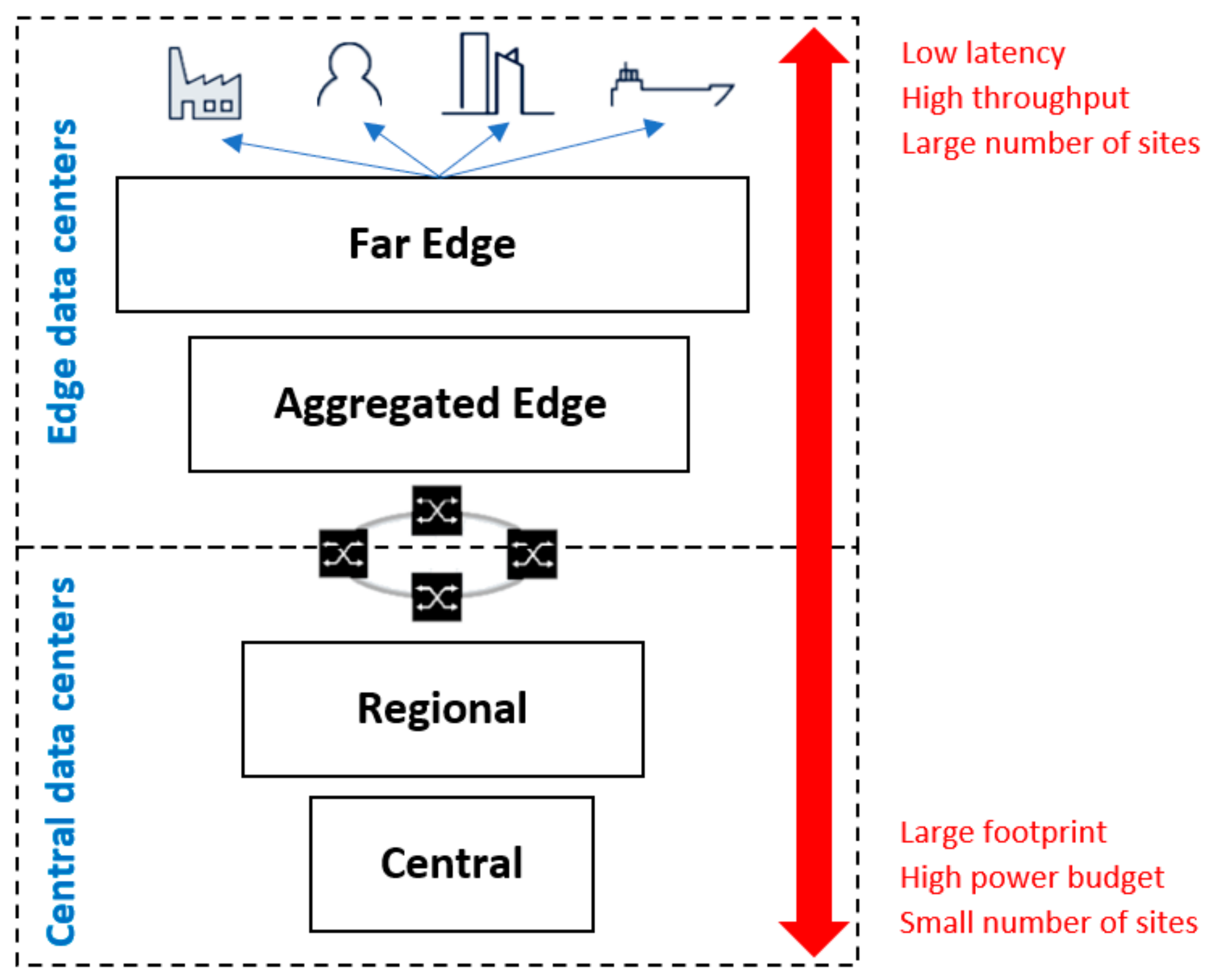
Figure 1.
Edge (MEC) and Central (Cloud) data centers.
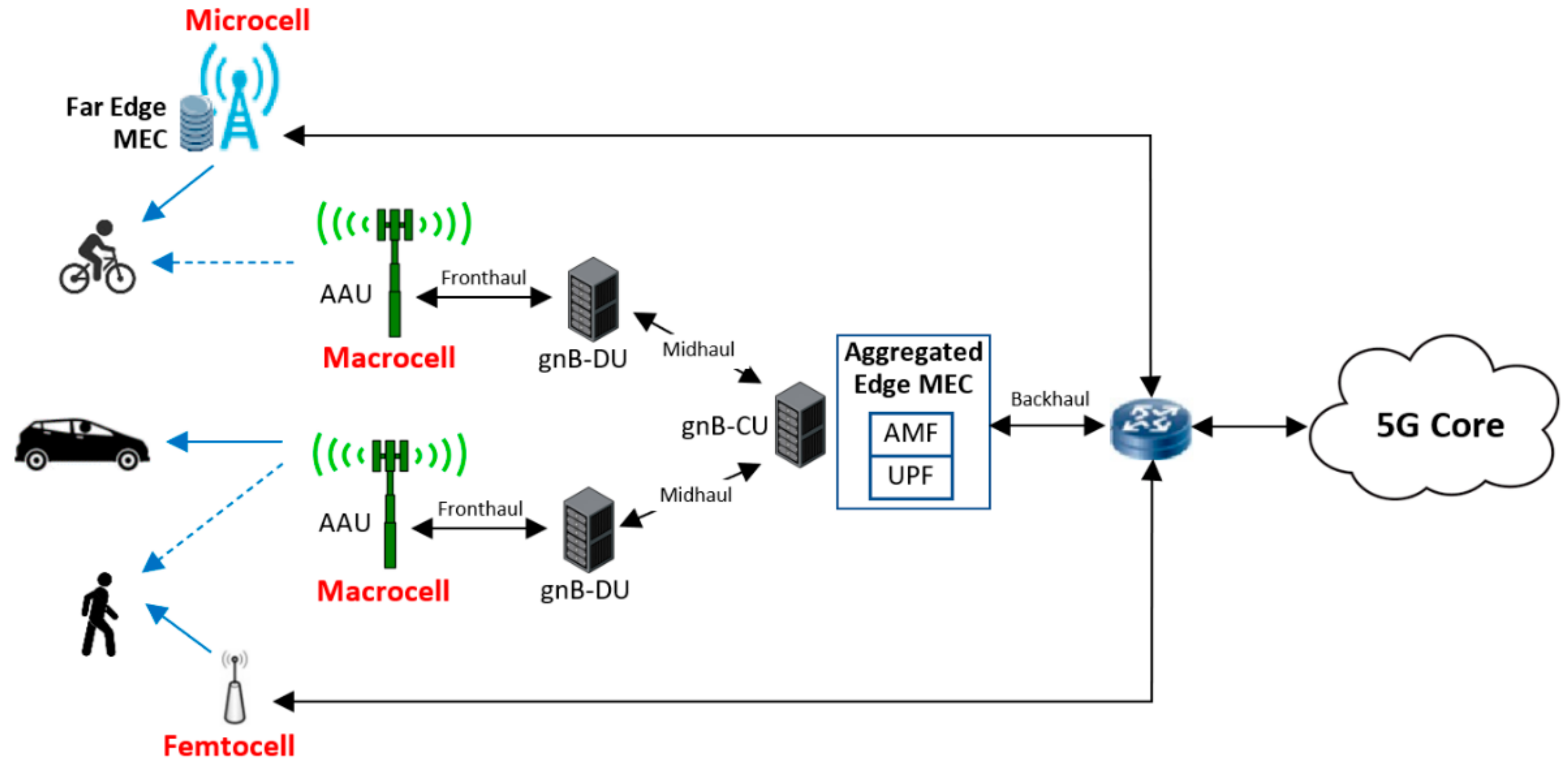
Figure 2.
Three-tier 5G RAN architecture with MEC deployment.
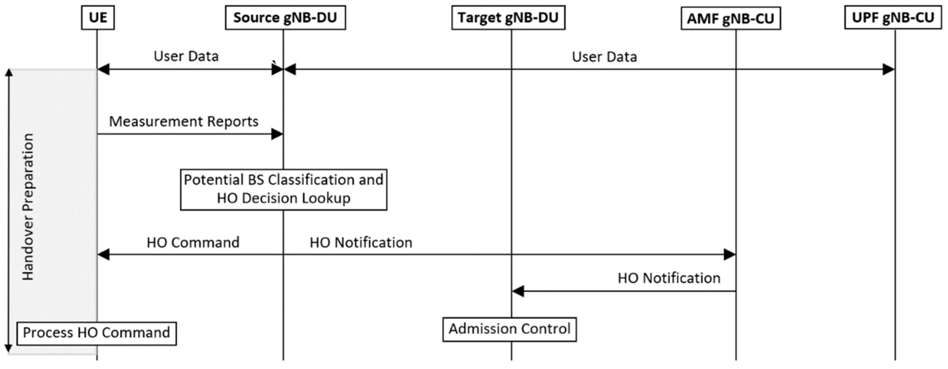
Figure 3.
Flow diagram of the modified handover preparation phase.
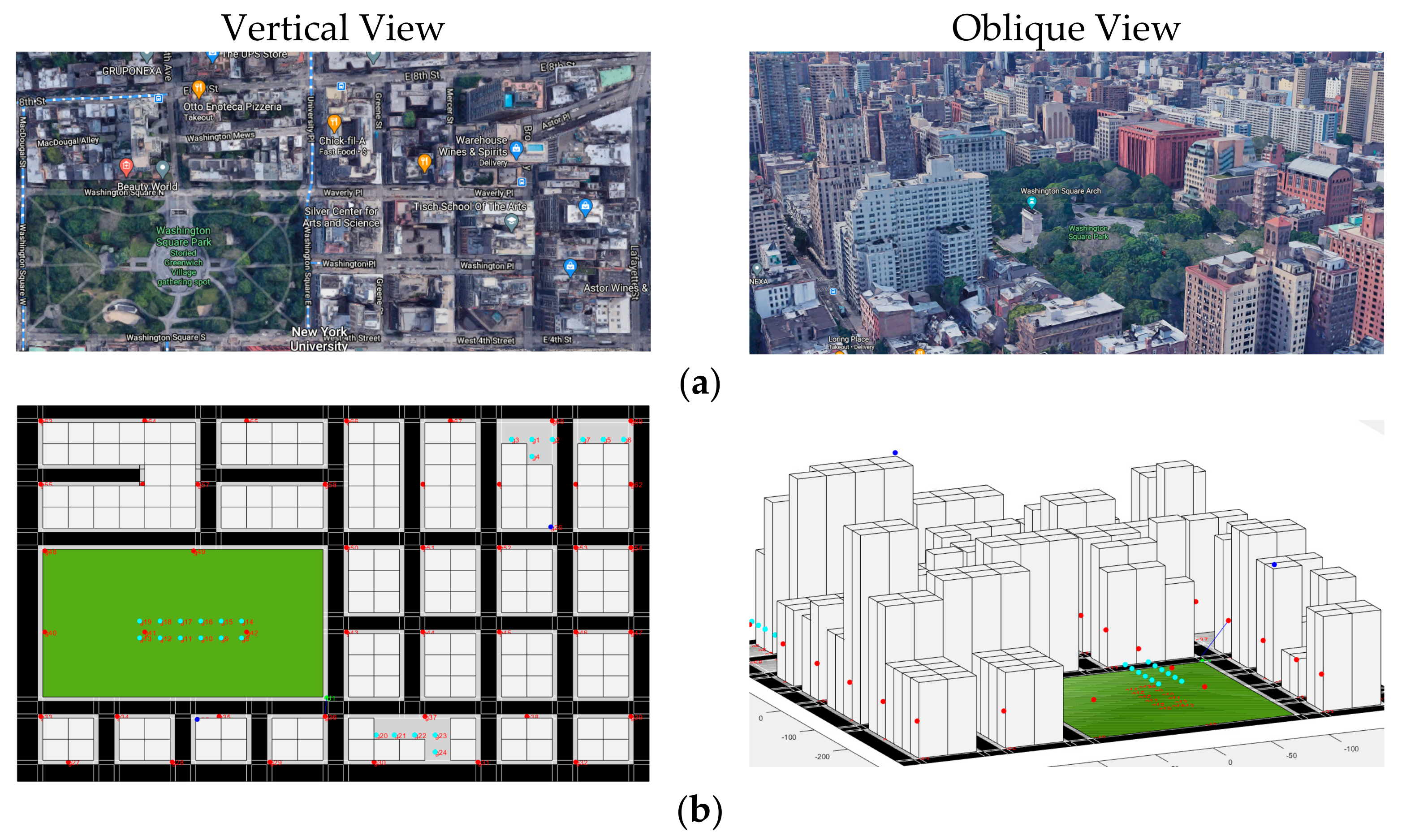
Figure 4.
(a) Vertical and oblique aerial views of the NYU campus; (b) Corresponding views of the simulated environment modeled after the NYU campus.
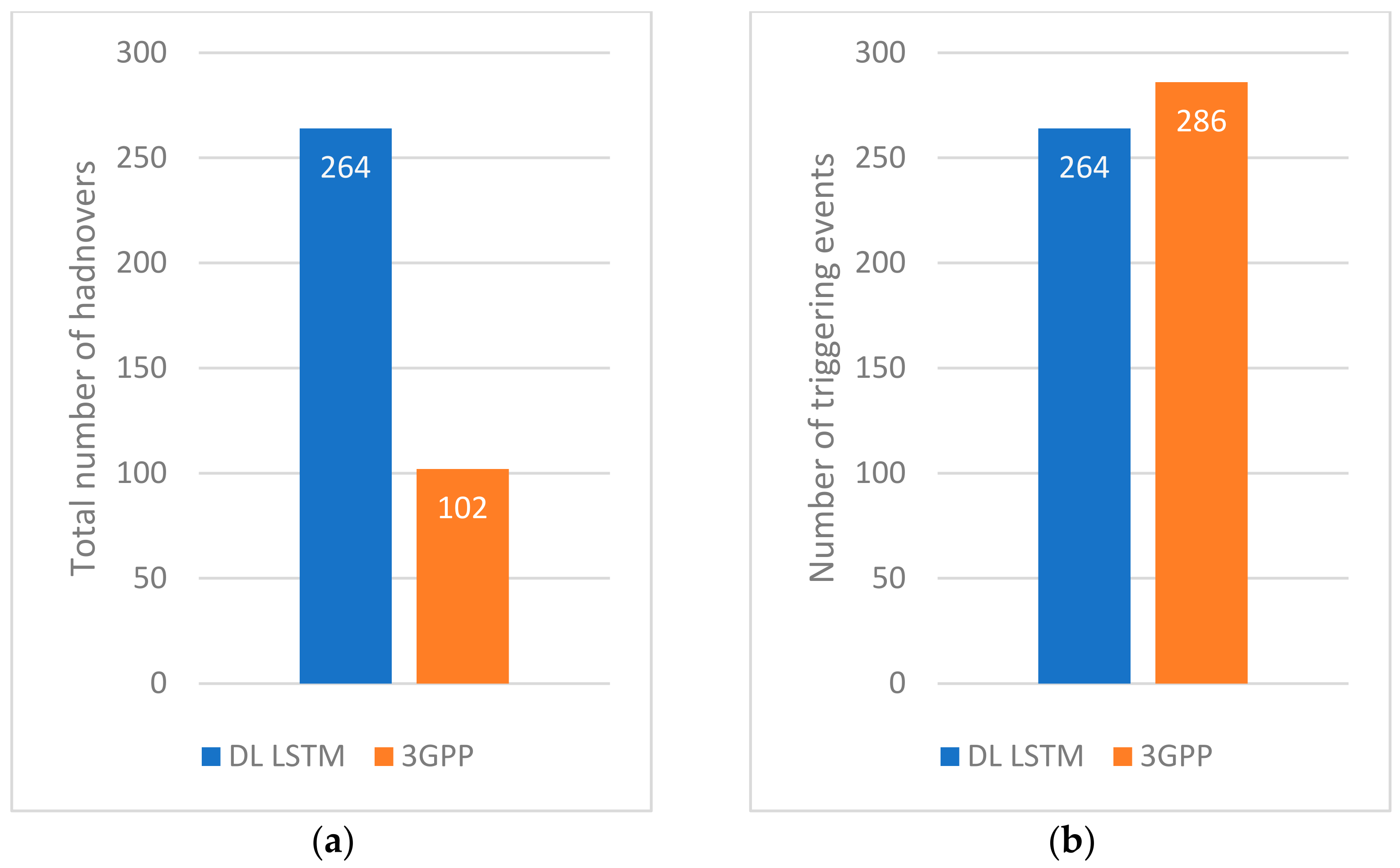
Figure 5.
(a) Total number of handovers and (b) number of triggering events.
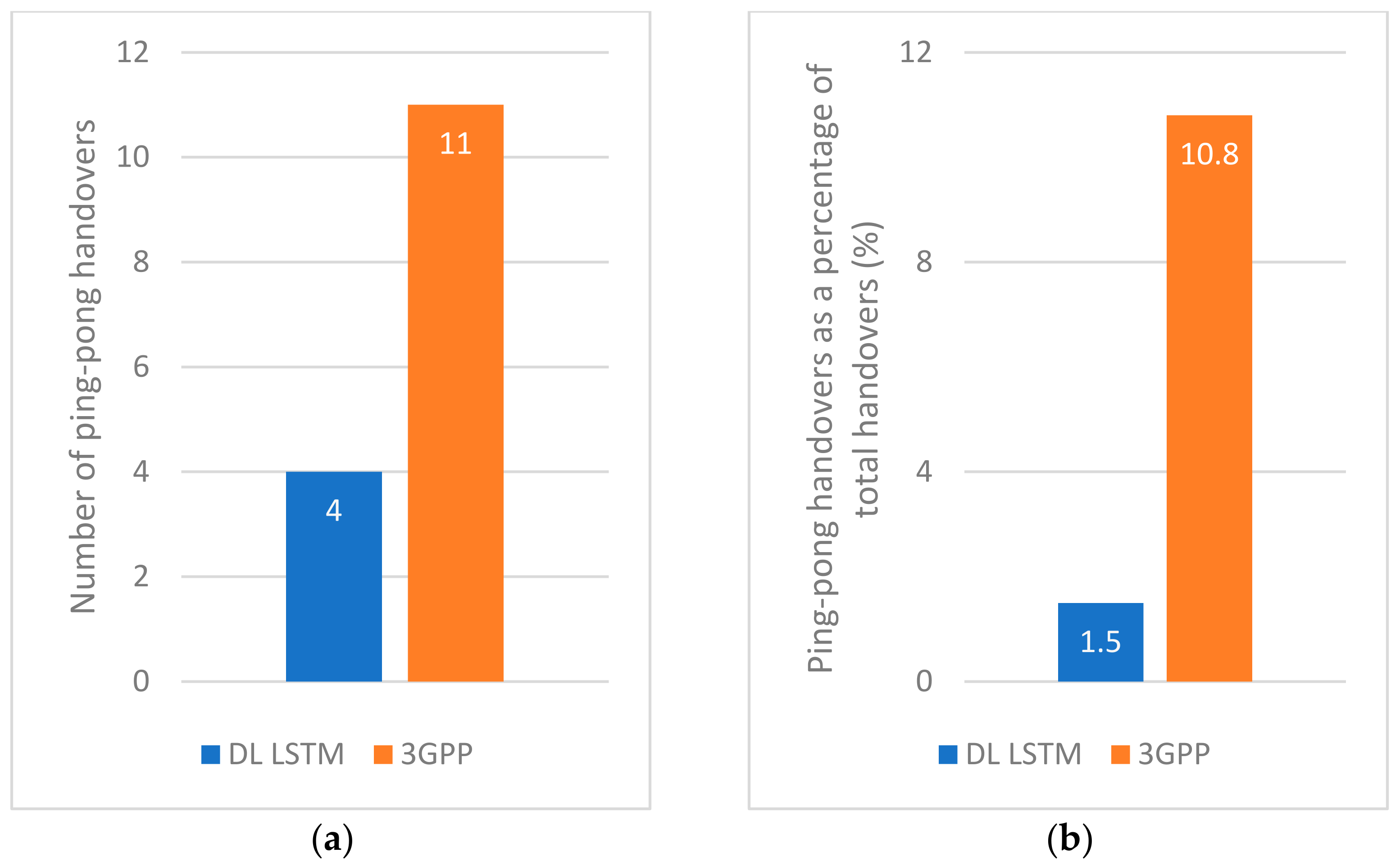
Figure 6.
(a) Number of ping-pong handovers and (b) ping-pong handovers as a percentage of total handovers.
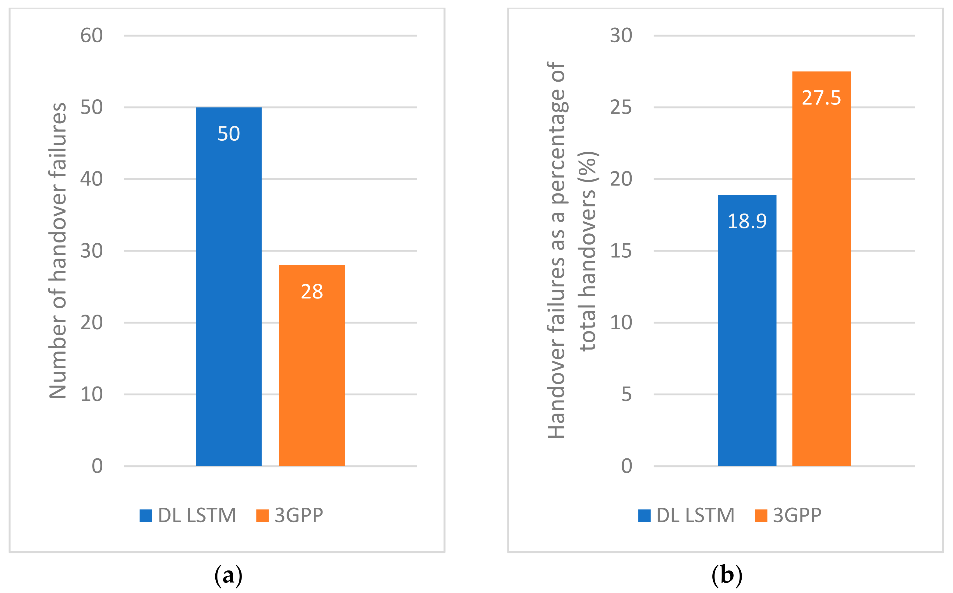
Figure 7.
(a) Number of handover failures and (b) handover failures as a percentage of total handovers.
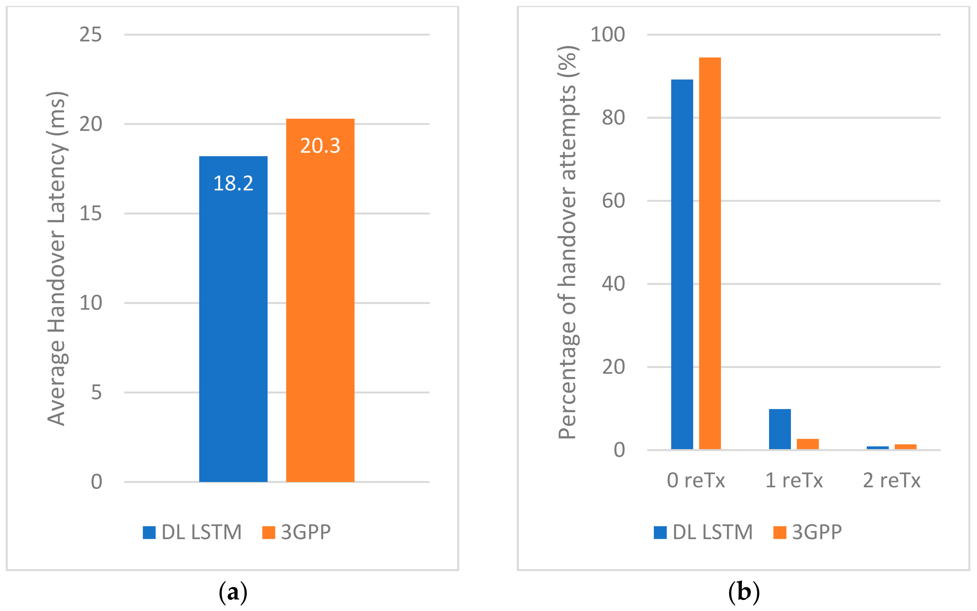
Figure 8.
(a) Average handover latency and (b) percentage of handover attempts.
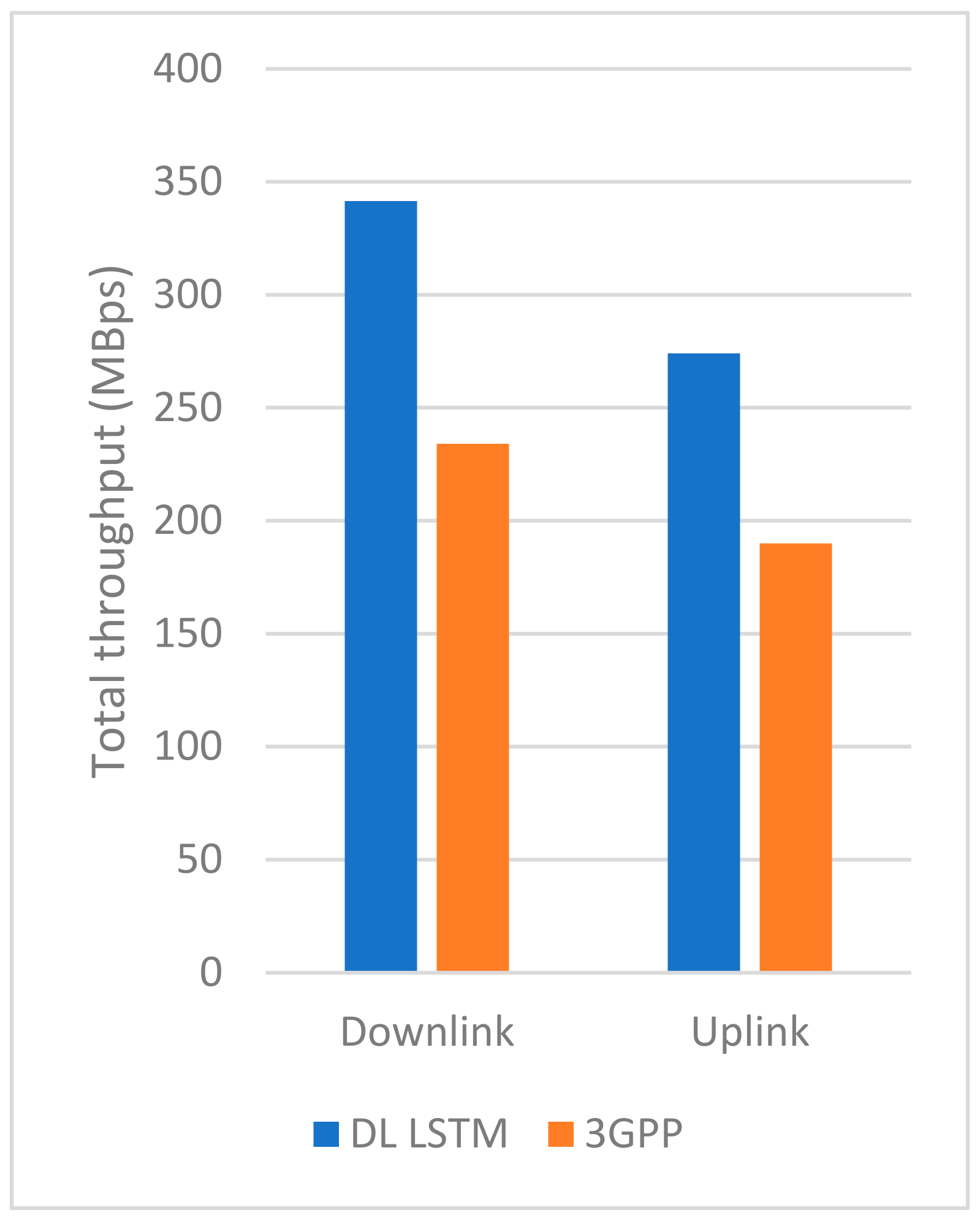
Figure 9.
Total throughput.
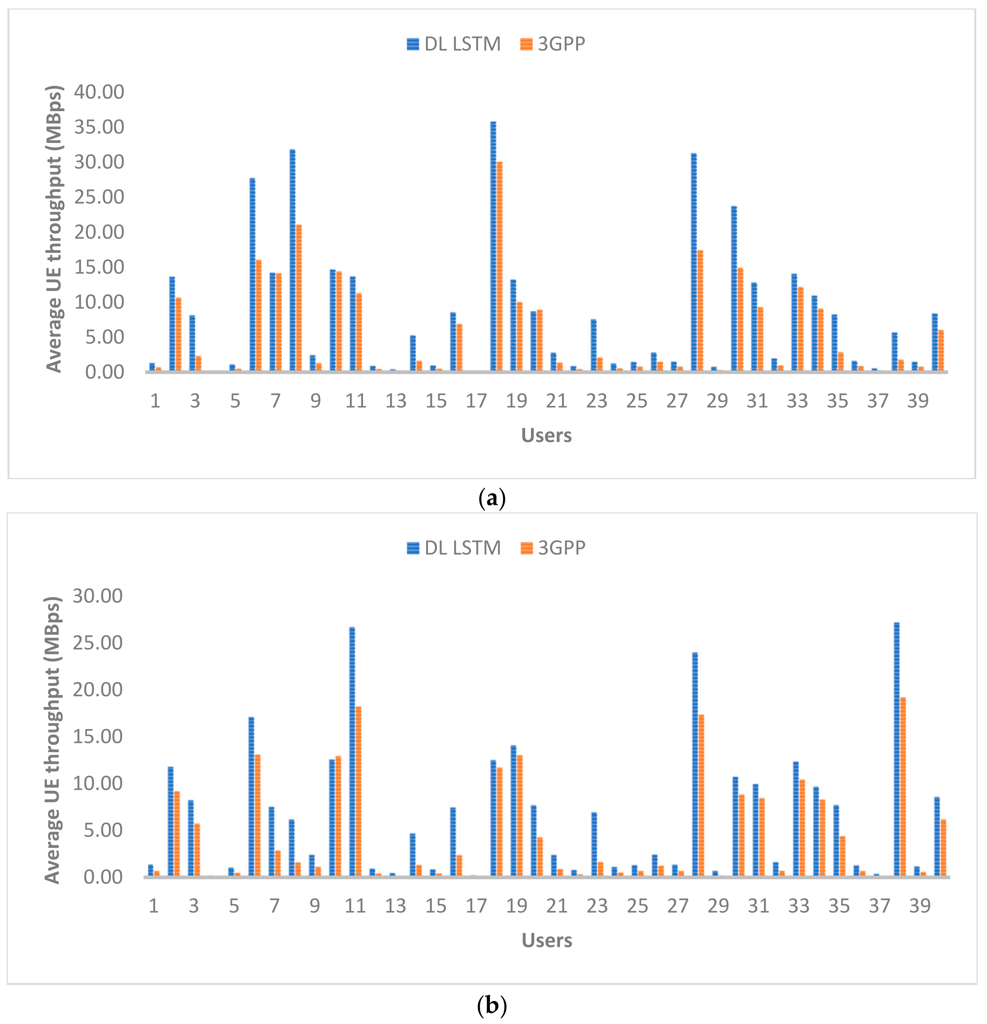
Figure 10.
Average UE throughput for (a) downlink and (b) uplink.
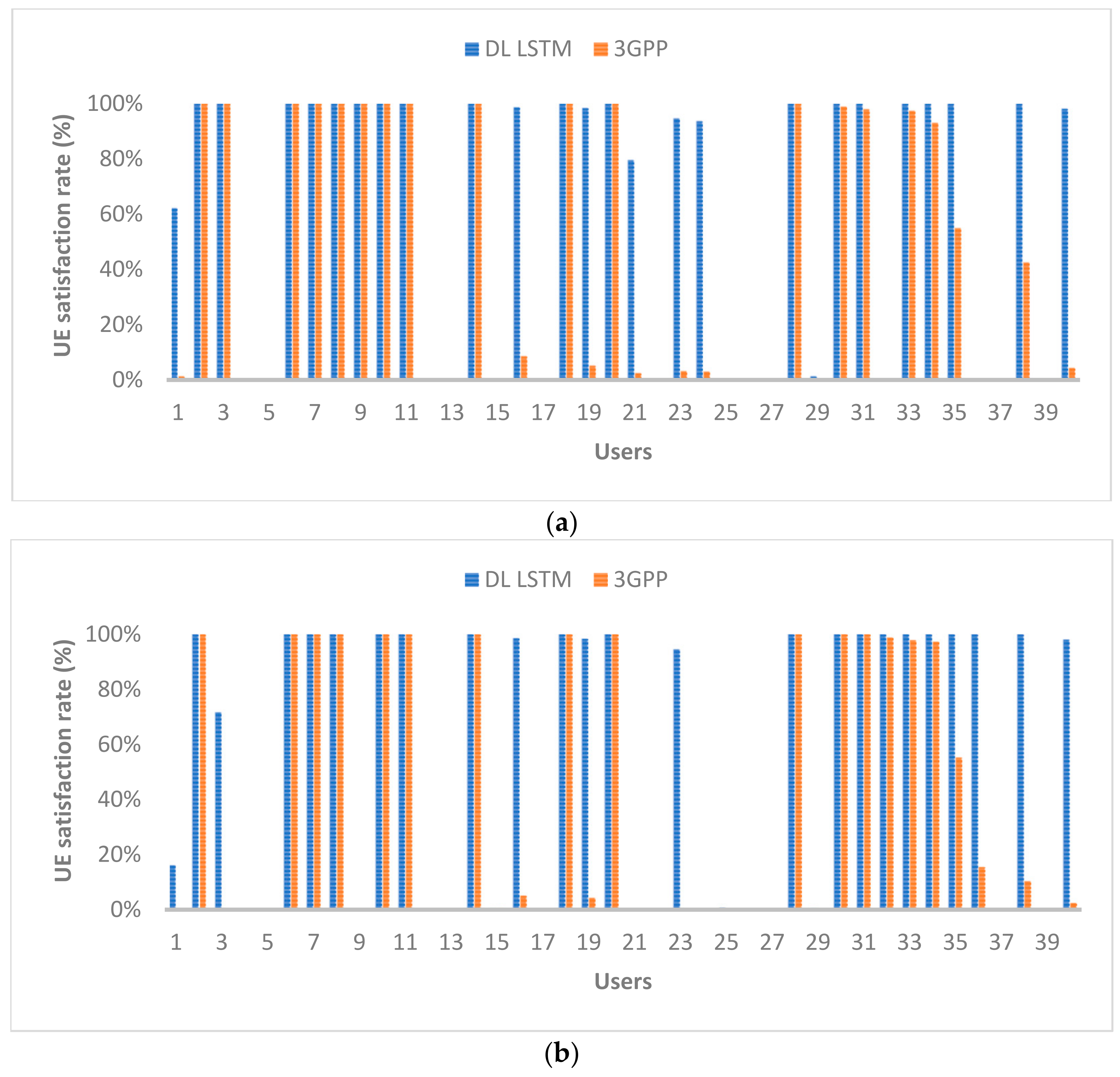
Figure 11.
UE satisfaction for (a) downlink and (b) uplink.
Table 1.
Handover trigger events for intra-RAT handover.
| Event | Description |
|---|
| A1 | Serving cell becomes better than a threshold |
| A2 | Serving becomes worse than a threshold |
| A3 | Neighbor becomes offset better than serving |
| A4 | Neighbor becomes better than a threshold |
| A5 | Serving cell becomes worse than threshold 1, and neighboring cell becomes better than threshold 2 |
| A6 | Neighbor become offset better than secondary cell |
Table 2.
Event parameter ranges.
| Event | Parameter | Minimum | Maximum |
|---|
| A1, A2, A4, A5 | RSRP threshold | −156 dBm | −31 dBm |
| All | Hysteresis | 0 dB | 15 dB |
| A3, A6 | Offset | −15 dB | +15 dB |
Table 3.
Summary of related works.
| Approach | Ref. | Solution Summary | Benefits and Drawbacks |
|---|
| Multi-connectivity | [15] | | Benefits:
Drawbacks:
High signaling overhead Inefficient use of radio resources No comprehensive study of multi-tier HOs despite having a two-tier scenario Focuses mainly on one tier and uses the other tier as a fall-back system
|
| [16] | |
| [17] | Proposes HO decision scheme for vehicles based on geometrically calculated cell coverage, vehicle trajectory, and HO latency Uses soft HO between RSUs and hard HO between RSU and BS
|
| AI-based | [18] | | Benefits:
Drawbacks:
|
| [19] | Proposes to use ML and data mining techniques to learn and identify cell characteristics and then optimize the HO parameters for in-building BSs The considered HO parameters are A2 and A3 handover thresholds, and TTT period
| Benefits:
Good throughput Low latency
Drawbacks:
No results on HOF, number of HOs, and ping-pong rates Only focused on exiting UEs
|
| [20] | Proposes a GRU-based scheme to predict the number of users in a cell for a given time of day The prediction is used for varying cell sizes, making it easier for UEs to be handed over to underloaded cells or harder for UEs to connect to overloaded cells
| Benefits:Drawbacks:
When all cells overloaded, radio link failures increase Need plenty of data to learn Lower accuracy than LSTMs
|
| [21] | | Benefits:
Drawbacks:
|
| Cloud/Edge-based | [22] | | Benefits:
Drawbacks:
|
| [23] | | Benefits:
Drawbacks:
|
| [24] | | Benefits:
Drawbacks:
|
Table 4.
A1 and A3 handover conditions.
| A3 Event | A1 Event |
|---|
| target gNB RSS > source gNB RSS + A3 offset (3 dB) | source gNB RSS > A1 threshold (minimum RSS for a CQI of 1) |
Table 5.
DL LSTM classification categories.
| Dimension | Classification | Letter Code | Value Range |
|---|
| User CQI | Good | G | CQI > 5 |
| Ok | O | 3 < CQI ≤ 5 |
| Poor | P | CQI ≤ 2 |
| User DRR | Met | M | DRR ≥ 1 |
| Not Met | N | DRR < 1 |
| User Direction | Closer | C | Δ RSS ≥ 0 dBm |
| Away | A | Δ RSS < 0 dBm |
| User Speed | Fast | F | |Δ RSS| ≥ 5 dBm |
| Low | L | |Δ RSS| < 5 dBm |
Table 6.
All 24 classification of the proposed DL LSTM.
| Index | Code | Classification |
|---|
| CQI | DRR | Direction | Speed |
|---|
| 1 | GMCF | Good | Met | Closer | Fast |
| 2 | GMCL | Low |
| 3 | GMAF | Away | Fast |
| 4 | GMAL | Low |
| 5 | GNCF | Not met | Closer | Fast |
| 6 | GNCL | Low |
| 7 | GNAF | Away | Fast |
| 8 | GNAL | Low |
| 9 | OMCF | Ok | Met | Closer | Fast |
| 10 | OMCL | Low |
| 11 | OMAF | Away | Fast |
| 12 | OMAL | Low |
| 13 | ONCF | Not met | Closer | Fast |
| 14 | ONCL | Low |
| 15 | ONAF | Away | Fast |
| 16 | ONAL | Low |
| 17 | PMCF | Poor | Met | Closer | Fast |
| 18 | PMCL | Low |
| 19 | PMAF | Away | Fast |
| 20 | PMAL | Low |
| 21 | PNCF | Not met | Closer | Fast |
| 22 | PNCL | Low |
| 23 | PNAF | Away | Fast |
| 24 | PNAL | Low |
Table 7.
LUT for handover decisions based on DL LSTM classifications.
| Classification for Potential BS | Parameters of Current BS |
|---|
| DR Met | DR Not Met |
|---|
| CQI < 3 | CQI ≥ 3 | CQI < 3 | CQI ≥ 3 |
|---|
| GMCF | 1 | 0 | 1 | 1 |
| GMCL | 1 | 0 | 1 | 1 |
| GMAF | 1 | 0 | 1 | 1 |
| GMAL | 1 | 0 | 1 | 1 |
| GNCF | 1 | 0 | 1 | 0 |
| GNCL | 1 | 0 | 1 | 0 |
| GNAF | 1 | 0 | 1 | 0 |
| GNAL | 1 | 0 | 1 | 0 |
| OMCF | 1 | 0 | 1 | 1 |
| OMCL | 1 | 0 | 1 | 1 |
| OMAF | 1 | 0 | 1 | 0 |
| OMAL | 1 | 0 | 1 | 1 |
| ONCF | 1 | 0 | 1 | 0 |
| ONCL | 1 | 0 | 1 | 0 |
| ONAF | 1 | 0 | 1 | 0 |
| ONAL | 1 | 0 | 1 | 0 |
| PMCF | 1* | 0 | 1* | 0 |
| PMCL | 1* | 0 | 1* | 0 |
| PMAF | 0 | 0 | 0 | 0 |
| PMAL | 0 | 0 | 0 | 0 |
| PNCF | 1* | 0 | 1* | 0 |
| PNCL | 1* | 0 | 1* | 0 |
| PNAF | 0 | 0 | 0 | 0 |
| PNAL | 0 | 0 | 0 | 0 |
Table 8.
BS simulation parameters.
| Parameters | Macro Cell (Wide Area BS) | Micro/Pico Cell (Medium Area BS) | Femtocell
(Local Area BS) |
|---|
| Number of BSs | 2 | 43 | 24 |
| BS coverage range | 500–1000 m | 50–100 m | 10–20 m |
| BS height | 50 m | 10 m | 6.5 m |
| Min distance to UE | 35 m | 5 m | 2 m |
| Carrier frequency | 2.0 GHz | 3.5 GHz | 26 GHz |
| Bandwidth | 20 MHz | 40 MHz |
| Duplex mode | FDD |
| Transmit power | 40 W | 6.31 W | 0.25 W |
| Antenna gain | 0 dBi |
| Number of antennas | 1 TX/RX pair |
| Pathloss model (LOS/NLOS) | 3D-UMa | 3D-UMi | Free-space + other loss factors * |
| Shadow fading | 4 dB |
| Wall losses | 13 dB |
Table 9.
UE simulation parameters.
| Parameters | Motorists | Cyclists | Pedestrians |
|---|
| Number of UEs | 22 | 4 | 14 |
| Speeds | 0−80 km/h | 0−20 km/h | 0−5 km/h |
| Channel model | Vehicle A | Typical Urban | Typical Urban |
| Number of antennas | 2 TX/RX pairs (one operates at 2/3.5 GHz; the other at 26 GHz) |
| Transmit power | 1 W |
Table 11.
Effects of the number of epochs (20 hidden units).
| Number of Epochs | Learning Time (s) | Prediction Accuracy (%) |
|---|
| Run 1 | Run 2 | Run 3 | Mean | Run 1 | Run 2 | Run 3 | Mean |
|---|
| 10 | 4 | 4 | 4 | 4 | 22.12 | 8.17 | 19.86 | 16.72 |
| 100 | 37 | 34 | 34 | 35 | 57.03 | 67.89 | 54.17 | 59.70 |
| 1000 | 352 | 353 | 360 | 355 | 99.45 | 99.86 | 99.47 | 99.59 |
| 2000 | 710 | 819 | 739 | 756 | 90.05 | 90.68 | 99.35 | 93.36 |
| Publisher’s Note: MDPI stays neutral with regard to jurisdictional claims in published maps and institutional affiliations. |
© 2021 by the authors. Licensee MDPI, Basel, Switzerland. This article is an open access article distributed under the terms and conditions of the Creative Commons Attribution (CC BY) license (https://creativecommons.org/licenses/by/4.0/).


