Comparison of the Methods for Predicting the Critical Temperature and Critical Pressure of Petroleum Fractions and Individual Hydrocarbons

Abstract

All modern process simulators rely on thermodynamic methods to estimate physical properties and calculate phase equilibria. The critical properties of individual components or pseudo-components, which represent undefined mixtures, play a crucial role in these calculations. However, the chemical compositions and characteristics of whole crude oils, petroleum fractions, and fuels, which are very complex mixtures of individual hydrocarbons, can vary significantly depending on the specific crude oil and the processing involved. For instance, straight-run petroleum fractions differ from those obtained through cracking processes due to differences in unsaturated hydrocarbon content. Consequently, effective methods for predicting critical temperature and pressure must account for a wide range of compositional scenarios. To address this challenge, we utilized a database of 176 individual hydrocarbons to evaluate the existing correlations for critical temperature and pressure calculations. Intercriteria analysis was performed to evaluate the relations between the different variables to be used for critical temperature and pressure predictions. Additionally, we proposed new correlations and ANN models for these properties and assessed their performance. Our study aims to provide robust predictive models that can accurately estimate critical properties across diverse petroleum fractions and compositions.

1. Introduction

The characterization of narrow petroleum fractions, particularly in relation to their individual hydrocarbon components, is crucial for accurate property estimation. Critical properties, such as critical temperature and pressure, are essential for these estimations. These properties can be obtained through direct measurement or predicted using thermodynamic correlations. For mixtures containing identifiable components, group-contribution methods, like those of Ambrose [1], Lydersen [2], and Nannoolal et al. [3], provide effective estimation techniques.

However, the full identification of all components in petroleum fractions is feasible only for lighter fractions, such as light naphtha. Heavier fractions contain more possible individual components, making their complete identification impractical. Historically, petroleum fraction identification relied on easily measurable properties, like the boiling point curve, specific gravity, and kinematic viscosity [4]. While these macroscopic properties are useful for initial characterization, they do not account for the intermolecular forces that control the behavior of individual components within a mixture.

Predicting critical properties based solely on boiling point and specific gravity is inherently empirical. The lack of theoretical background means such correlations may fail outside their development data range [4]. Hajipour and Satyro emphasize this issue, noting that small errors in critical properties used in equations of state can dramatically affect the final results. For example, underestimating the critical temperature by 2% can lead to vapor pressure prediction errors between 20% and 60% [5].

Another challenge in measuring or predicting critical properties is the decomposition of heavier hydrocarbons at temperatures above 360 °C. As the normal boiling point approaches this threshold, the critical temperature exceeds 400 °C, making direct measurement impractical. Therefore, critical parameters are often fitted against vapor pressure data, as described by Kumar and Okuno [6]. This approach can be optimized for specific equations of state, such as the Peng–Robinson equation.

Several authors have summarized the available correlations for predicting the critical temperature and pressure of individual hydrocarbons and petroleum fluids. M.R. Riazi discusses several widely used methods in his work [7], including the Riazi–Daubert method [8] (adopted by API and recommended for use in API-TDB [9]), the Lee–Kesler method [10], the Cavett method [11], the Twu method [12] (recommended by many process simulator vendors), the Winn–Mobil method [13], and a correlation developed by Tsonopoulos et al. [14] specifically for coal liquids and fractions rich in aromatics.

A more recent study by Hosseinifar and Jamshidi [15] evaluates critical properties using experimental data from 255 pure substances and 50 petroleum fractions, proposing a method that calculates critical properties and the acentric factor using molecular weight and refractive index or boiling point and refractive index as parameters. They summarize the use of various compound types: 75 alkanes, 23 alkenes, 12 alkynes, 17 alkanols, 27 esters, 10 ethers, 16 ketones, 14 sulfides, 17 plasticizers, 12 benzene derivatives, 18 poly-nuclear aromatics, and 14 halogenated hydrocarbons.

Table 1. Summary of the available correlations for the estimation of the critical temperature and critical pressure of petroleum fractions and hydrocarbons.

Source (Year of Publication)	Correlation	Range of Applicability	Equation
Winn–Mobil (1957) [13]	$\ln T_c=-0.58779+4.2009T_b^{0.08615}{SG}^{0.04614}$ $P_c=6.148314\times {10}^7{T}_b^{-2.3177}{SG}^{2.4853}$	Based on Winn’s nomogram 80 F < MABP < 1200 F 80 < MW < 600	(1)
Cavett (1962) [11]	$T_c=426.7062278+9.5187183\times {10}^{-1}{T}_b-6.01889\times {10}^{-4}{T}_b^2-4.95625\times {10}^{-3}API T_b+2.160588\times {10}^{-7} T_b^3+2.949718\times {10}^{-6} API T_b^2+1.817311\times {10}^{-8}{API}^2 T_b^2$ ${\mathrm{l}\mathrm{o}\mathrm{g}(P}_c)=1.6675956+9.412011\times {10}^{-4} T_b-3.047475\times {10}^{-6}{T}_b^2-2.087611\times {10}^{-5}API T_b+1.5184103\times {10}^{-9}{T}_b^3+1.1047899\times {10}^{-8}API T_b^2-4.8271599\times {10}^{-8}{API}^2{T}_b+1.3949619\times {10}^{-10}{API}^2 T_b^2$ $API={\displaystyle \frac{141.5}{SG}}-131.5$ Tb is in degrees Fahrenheit		(2)
Lee–Kesler (1976) [10]	$T_c=189.8+450.6\times SG+\left(0.4244+0.1174\times SG\right)\times T_b+{\displaystyle \frac{\left(0.1441-1.0069\times SG\right)\times {10}^5}{T_b}}$ $\ln \left(P_c\right)=5.689-{\displaystyle \frac{0.0566}{SG}}-\left(0.43639+{\displaystyle \frac{4.1216}{SG}}+{\displaystyle \frac{0.21343}{{SG}^2}}\right)\times {10}^{-3} T_b+\left(0.47579+{\displaystyle \frac{1.182}{SG}}+{\displaystyle \frac{0.15302}{{SG}^2}}\right)\times {10}^{-6} T_b^2-\left(2.4505+{\displaystyle \frac{9.9099}{{SG}^2}}\right)\times {10}^{-10}\times T_b^3$	70 < MW < 700 C5 ÷ C50	(3)
Riazi–Daubert (1980) [8]	$T_c=19.06232\times T_b^{0.58848}{\times SG}^{0.3596}$ $P_c=5.53027\times {10}^7\times T_b^{-2.3125}{\times SG}^{2.3201}$	70 < MW < 700	(4)
Riazi (1987) [7]	$T_c=9.5233\times \left[\exp \left(-9.314\times {10}^{-4}\times T_b-0.54442\times SG+6.4791\times {10}^{-4} {\times T}_b\times SG\right)\right]\times T_b^{0.81067}{\times SG}^{0.53691}$ $P_c=3.1958\times {10}^5\times \left[\exp \left(-8.505x\times T_b-4.8014\times SG+5.749x\times T_b\times SG\right)\right]\times T_b^{-0.4844}\times {SG}^{4.0846}$ $T_c=35.9413\times \left[\exp \left(-6.9\times {10}^{-4}\times T_b-1.4442 SG+4.91\times {10}^{-4} T_b\times SG\right)\right]{\times T}_b^{0.7293}{\times SG}^{1.2771}$ $P_c=6.9575\times \left[\exp \left(-1.35\times {10}^{-2}\times T_b-0.3129\times SG+9.174\times {10}^{-3}{T}_b\times SG\right)\right]\times T_b^{0.6791}{\times SG}^{-0.6807}$	70 < MW < 700 >C20	(5)
Tsonopoulos (1986) [14]	${log}_{10}\left(T_c\right)=1.20016+0.61954\times {log}_{10}\left(T_b\right)+0.48262\times {log}_{10}\left(SG\right)+0.67365\times {{(log}_{10}\left(SG\right))}^2$ ${log}_{10}\left(P_c\right)=7.37498-2.15833\times {log}_{10}\left(T_b\right)+3.35417\times {log}_{10}\left(SG\right)+5.64019\times {{(log}_{10}\left(SG\right))}^2$	Coal liquid fractions high in aromatic hydrocarbons	(6)
Twu (1987) [12]	$T_c^o=T_b\times (0.533272+0.34383\times {10}^{-3}{T}_b+2.52617\times {10}^{-7} T_b^2-1.658481\times {10}^{-10} {\times T}_b^3+4.60772\times {10}^{24}\times T_b^{-13}{)}^{-1}$ $\alpha =1-T_b/T_c^o$ $P_c^o=(1.00661+0.31412\times {\alpha }^{0.5}+9.16106\times \alpha +9.5041\times {\alpha }^2+27.3588 {\times \alpha }^4{)}^2$ $V_c^0=(0.34602+0.30171\times \alpha +0.93307\times {\alpha }^3+5655.414\times {\alpha }^{14}{)}^{-8}$ ${SG}^o=0.843593-0.128624\times \alpha -3.36159\times {\alpha }^3-13749.5\times {\alpha }^{12}$ $\mathsf{\Delta }{SG}_T=\exp \left[5\left({SG}^o-SG\right)\right]-1$ $f_T=\mathsf{\Delta }{SG}_T[-{\displaystyle \frac{0.27016}{T_b^{0.5}}}+\left(0.0398285-{\displaystyle \frac{0.706691}{T_b^{0.5}}}\right)\times \mathsf{\Delta }{SG}_T]$ $T_c=T_c^o[{\displaystyle \frac{1+2 f_T}{1-2 f_T}}{]}^2$ $\mathsf{\Delta }{SG}_V=\exp \left[4\left({SG}^{o2}-{SG}^2\right)\right]-1$ $f_V=\mathsf{\Delta }{SG}_V\times \left[{\displaystyle \frac{0.347776}{T_b^{0.5}}}+\left(-0.182421+{\displaystyle \frac{2.248896}{T_b^{0.5}}}\right)\times \mathsf{\Delta }{SG}_V\right]$ $V_c=V_c^o[{\displaystyle \frac{1+2 f_V}{1-2 f_V}}{]}^2$ $\mathsf{\Delta }{SG}_P=\exp \left[0.5\left({SG}^o-SG\right)\right]-1$ $f_P=\mathsf{\Delta }{SG}_P\left[\left(2.53262-{\displaystyle \frac{34.4321}{T_b^{0.5}}}-2.30193{\displaystyle \frac{{\mathrm{T}}_b}{1000}}\right)+(-11.4277+{\displaystyle \frac{187.934}{T_b^{0.5}}}+4.11963{\displaystyle \frac{{\mathrm{T}}_b}{1000}})\times \mathsf{\Delta }{SG}_P\right]$ $P_c=P_c^o\times \left({\displaystyle \frac{T_c}{T_c^o}}\right)\times \left({\displaystyle \frac{V_c^o}{V_c}}\right)\times [{\displaystyle \frac{1+2 f_p}{1-2 f_p}}{]}^2$		(7)
Lin–Chao (1984) [16]	$T_{cA}=2.72697\times {10}^2+3.91999\times M-1.17706\times {10}^{-2}{M}^2+1.48679\times {10}^{-5}\times M^3-{\displaystyle \frac{2.27789\times {10}^3}{M}}$ $\ln \left(P_{cA}\right)=1.77645-1.01820\times {10}^{-2}\times M+2.51106\times {10}^{-5}{M}^2-3.73775\times {10}^{-8} M^3-{\displaystyle \frac{3.50737}{M}}$ ${SG}_A=0.66405+1.48130\times {10}^{-3}\times M-5.07021\times {10}^{-6}{\times M}^2+6.21414\times {10}^{-9}{\times M}^3-{\displaystyle \frac{8.45218}{M}}$ $T_{bA}=133.832+3.11349\times M-7.08978\times {10}^{-3}{\times M}^2+7.69085\times {10}^{-6}\times M^3-{\displaystyle \frac{1127.31}{M}}$ $\mathsf{\Delta }SG=SG-{SG}_A; \mathsf{\Delta }{T}_b=T_b-T_{bA}$ $T_c=T_{cA}+\left(1580.25-11.8432\times M\right)\times \mathsf{\Delta }SG+\left(-5.68509+5.77384\times {10}^{-2}\times M\right)\times \mathsf{\Delta }{T}_b+\left(-12165.9+110.697\times M\right){\times \left(\mathsf{\Delta }SG\right)}^2+\left(75.0653-0.65845\times M\right)\times \mathsf{\Delta }SG\mathsf{\Delta }{T}_b+(-9.66385\times {10}^{-2}+7.8231\times {10}^{-4}\times M)\times (\mathsf{\Delta }{T}_b{)}^2+(21711.2-204.245\times M)\times (\mathsf{\Delta }SG{)}^3+\left(-157.999+1.32064\times M\right){\times \left(\mathsf{\Delta }SG\right)}^2\times \mathsf{\Delta }{T}_b+(0.360522-2.27593\times {10}^{-3}M)\times \mathsf{\Delta }SG\times (\mathsf{\Delta }{T}_b{)}^2+(-2.75762\times {10}^{-4}+8.74295\times {10}^{-7}\times M)\times (\mathsf{\Delta }{T}_b{)}^3$ ${\mathrm{l}\mathrm{n}(P}_c)={\mathrm{l}\mathrm{n}(P}_{cA})+\left(9.71572-7.5037\times {10}^{-2}M\right)\times \mathsf{\Delta }SG+\left(-3.32004\times {10}^{-2}+3.15717\times {10}^{-4}M\right)\times \mathsf{\Delta }{T}_b+\left(-86.0375+0.84854\times M\right)\times {\left(\mathsf{\Delta }SG\right)}^2+\left(0.550118-5.21464\times {10}^{-3}\times M\right)\times \mathsf{\Delta }SG\mathsf{\Delta }{T}_b+(-9.00036\times {10}^{-4}+7.87325\times {10}^{-6}\times M)\times (\mathsf{\Delta }{T}_b{)}^2+(185.927-1.85430\times M)\times (\mathsf{\Delta }SG{)}^3+\left(-1.51115+1.36051\times {10}^{-2}\times M\right)\times {\left(\mathsf{\Delta }SG\right)}^2\times \mathsf{\Delta }{T}_b+(4.32808\times {10}^{-3}-3.23929\times {10}^{-5}\times M)\times \mathsf{\Delta }SG\times (\mathsf{\Delta }{T}_b{)}^2+(-3.81526\times {10}^{-6}+2.18899\times {10}^{-8}\times M)\times (\mathsf{\Delta }{T}_b{)}^3$ Tc and Tb are in Kelvin; Pc is in MPa		(8)
Jianzhong et al. (1998) [17]	$T_c=18.2394\times T_b^{0.595251}{\times SG}^{0.34742}$ $P_c=0.295152\times T_b^{-2.2082}{\times SG}^{2.22086}$ Tc and Tb are in Kelvin; Pc is in MPa		(9)
Hosseinifar (2014) [15]	$f\left(SG\right)=\sqrt{{\displaystyle \frac{3+2 SG}{3-SG}}}$ Critical properties based on MW: $T_c=(a\times [f\left(SG\right){]}^b{\times MW}^c+d\times [f\left(SG\right){]}^e{\times MW}^f{)}^g$ a = −9.45549; b = 6.98465; c = −1.31059; d = 6.34728; e = 0.54432 f = 0.09807; g = 2.55998 $P_c=(a\times [f\left(SG\right){]}^b\times {MW}^c+d\times [f\left(SG\right){]}^e\times {MW}^f{)}^g$ a = 0.06878; b = −1.03534; c = 0.37339; d = 18.73579; e = 3.34733 f = −2.03812; g = −2.6534 Critical properties based on Tb: $T_c=(a\times [f\left(SG\right){]}^b\times T_b^c+d\times [f\left(SG\right){]}^e{\times T}_b^f{)}^g$ a = −0.0419; b = −1.47872; c = 2.73355; d = 2.45861; e = −0.35125 f = 2.09619; g = 0.50569 $P_c=(a\times [f\left(SG\right){]}^b\times T_b^c+d\times [f\left(SG\right){]}^e\times T_b^f{)}^g$ a = −41.24678; b = 2.55879; c = −1.02425; d = 7.29072; e = 0.66689 f = −0.28966; g = 9.70427		(10)

provides a summary of the correlations used for predicting critical temperature and pressure from 1957 to 2025.

Table 1 details the existing methods, where, in the column “Range of Applicability”, the hydrocarbon boiling range, molecular weight, and carbon atom count given by the respective authors of the correlations are provided. The correlation given by Tsonopoulos, in particular, was developed for coal liquid fractions, which are typically high in aromatic hydrocarbon content. In general, all correlations mentioned above should be capable of predicting the critical properties of any of the classes of the hydrocarbons—n-alkanes, iso-alkanes, alkenes, alkynes, and mono- and poly-aromatic hydrocarbons. Considering that the mentioned correlations are used for the prediction of pseudo-component critical properties in commercial process simulators using only distillation curve data and bulk specific gravity, they shall be capable of predicting these critical properties for a wide variety of refinery products. As no data were found on the performance of a specific correlation in predicting the critical properties for the variety of compounds, we decided to perform a critical evaluation of the performance of these correlations in predicting the critical properties of a wide spectrum of individual hydrocarbon compounds.

2. Materials and Methods

In this study, we evaluate the existing correlations for predicting critical temperature and pressure using a comprehensive database of pure hydrocarbon components provided by Hajipour and Satyro [5]. This database includes 176 individual hydrocarbons with parameters critically evaluated and uncertainties in the determination for each substance. The dataset encompasses various types of components:

• 24 n-alkanes;
• 24 alkenes;
• 41 iso-alkanes;
• 16 iso-alkenes;
• 17 cyclo-alkanes;
• 5 cyclo-alkenes;
• 32 mono-aromatic compounds;
• 6 bicyclic hydrocarbons;
• 7 di-aromatic compounds;
• 3 tri-aromatic compounds;
• 1 tricyclic compound.

This extensive database provides a robust foundation for evaluating the performance of various correlations and developing new empirical methods.

The pure hydrocarbon component database used in this study is based on the publication by Hajipour and Satyro [5], where the authors critically evaluated the parameters of the hydrocarbons, with the uncertainties in the determination of the properties for each substance calculated. The critical properties are directly measured only for the light hydrocarbons, while for the heavy hydrocarbons, whose critical temperature exceeds 360 °C, their determination is performed by using indirect measurements—e.g., using and extrapolating pure component vapor pressure data. The uncertainties in critical properties determined in this way are very useful when making comparisons between correlations calculated by critical properties and measured ones using direct or indirect methods. We employed the database discussed in the work by Hajipour and Satyro [5] because the errors in the calculated critical properties can be compared with the uncertainty reported by Hajipour and Satyro for this database. This is the reason why we selected this dataset over the available bigger databases like the DIPPR database of AIChE.

The assessment of relationships between the characteristics that can be used for the purpose of predicting critical temperature and critical pressure was performed by using intercriteria analysis (ICrA) [18]. Details of the theory and application of ICrA are presented in ref. [19]. The ICrA approach calculates two intuitionistic fuzzy functions, i.e., μ and υ, whose values define the degree of the relationship between the criteria.

For μ = 0.75 ÷ 1.00 and υ = 0 ÷ 0.25, a region of statistically meaningful positive consonance is determined, while at μ = 0 ÷ 0.25 and υ = 0.75 ÷ 1.00, an area of statistically meaningful negative consonance is derived. All other cases are considered to be dissonance. A strong consonance is considered at values of μ = 0.95 ÷ 1.00, υ = 0.00 ÷ 0.05 (positive), μ = 0.00 ÷ 0.05, and υ = 0.95 ÷ 1.00 (negative), while a weak consonance is deemed at μ = 0.75 ÷ 0.85, υ = 0.15 ÷ 0.25 (positive), μ = 0.15 ÷ 0.25, and υ = 0.75 ÷ 0.85 (negative). Two software packages for ICrA were established and are freely available as open source from https://intercriteria.net/software/, accessed on 23 April 2025, as detailed in refs. [20,21,22].

In order to estimate parameters that have different dimensions, it is necessary to perform normalization over each criterion. The goal of the normalization process before performing ICrA is to transform features to be on a similar scale. This condition requires the use of Min-Max normalization. It allows the elements to converge more quickly during training, helps the method infer better estimations, and assists the method in learning appropriate weights for each feature. Therefore, before the ICrA evaluation, all variables were normalized using the normalization formula (Equation (11)).

$$X_{new}={\displaystyle \frac{X-X_{min}}{X_{max}-X_{min}}}$$

(11)

where X is the current estimation, X_min is the minimum value of all values in the estimated criteria column, and X_max is the maximum value of all values in the estimated criteria column. The normalization formula is used to unify all the values into the range [0,1]. Thereafter, the ICrA can estimate effectively the relationships between the criteria. The problem is discussed in ref. [23].

All correlations mentioned in Table 1 were evaluated using this dataset of 176 pure hydrocarbon components. The database was also used to perform regression analyses, which resulted in the development of new empirical correlations for predicting critical temperature and pressure. These newly developed correlations were then evaluated alongside those detailed in Table 1.

To assess the performance of both the existing correlations (Table 1) and the new empirical correlations presented here, we employed a series of statistical parameters. Specifically, these evaluations and ANN models were conducted using Equations (12)–(17), which include metrics such as:

$$Error \left(E\right):E=\left({\displaystyle \frac{{\xi }_{exp}-{\xi }_{calc}}{{\xi }_{exp}}}\right)\times 100$$

(12)

$$Standard error:{SE}_i=(\sum \left({\displaystyle \frac{{(\xi }_{exp }-{\xi }_{calc}{)}^2}{N-2}}\right){)}^{{\displaystyle \frac{1}{2}}}$$

(13)

$$Relative standard error \left(RSE\right): {RSE}_i={\displaystyle \frac{{SE}_i}{mean of the sample}}\times 100$$

(14)

$$Sum of square errors \left(SSE\right): SSE=\sum {\displaystyle \frac{1}{{\xi }_{exp}^2}}\times ({\xi }_{exp}-{\xi }_{calc}{)}^2$$

(15)

$$Average absolute deviation \left(\%AAD\right): \%AAD={\displaystyle \frac{1}{N}} {\displaystyle \frac{\sum |{\xi }_{exp}-{\xi }_{calc}|}{{\xi }_{exp}}}\times 100$$

(16)

$$Sum of relative errors \left(SRE\right): SRE=\sum \left({\displaystyle \frac{{\xi }_{exp}-{\xi }_{calc}}{{\xi }_{exp}}}\right)\times 100$$

(17)

where ξ_exp is the experimental value of the critical temperature or critical pressure; ξ_calc is the calculated value of the critical temperature or critical pressure; and N is the number of the experimental points.

These statistical parameters allow for a comprehensive evaluation of the accuracy, precision, and reliability of the correlations. The results will provide insights into which methods perform best under different conditions, thereby informing future improvements in thermodynamic modeling for petroleum fractions.

The use of artificial neural networks exploits the natural connectivity of individual neurons to create an architecture for predicting critical temperature and critical pressure. The ANN modeling was performed by using Matlab 2020 software. The training, validation, and test sets of the data used by the ANN were divided as follows: 70% for training; 20% for testing; and 10% for validation. In ANN modeling, the architecture of the network has a pivotal role. In this research, to model the critical temperature and critical pressure, we used an ANN consisting of six layers with the following structure: 64, 32, 16, 10, 8, and 1 neurons. That is, the first layer contains 64 neurons, the second contains 32, the third contains 16, the fourth contains 10, the fifth contains 8, and the sixth (output) contains 1. This architecture was chosen to efficiently process 5 × 176 input data. The number of neurons in each successive layer is approximately halved, starting from 64 neurons in the first layer. This configuration is considered optimal for capturing the essential features of the input data. Increasing the number of neurons leads to information redundancy and consequently to an increase in mean squared error (MSE), which negatively affects the modeling performance.

3. Results

The database of 176 pure hydrocarbons, critically evaluated by Hajipour and Satyro [5], was used for the purposes of this study. The five input variables used for the critical temperature and critical pressure predictions were boiling point, specific gravity, molecular weight, H/C atomic ratio, and acentric factor (Omega). The evaluation of the ICrA of the data for these variables, along with the data for the critical temperature in terms of μ and υ-values, is summarized in

Table 2. μ-values from the ICrA evaluation of the data for the 176 pure hydrocarbons used in this research for the purpose of modeling the critical temperature.

μ	Tb (K)	SG	MW	H/C Ratio	Omega	Tc (K)
Tb (K)	1.00	0.77	0.89	0.31	0.81	0.94
SG	0.77	1.00	0.69	0.14	0.62	0.81
MW	0.89	0.69	1.00	0.39	0.82	0.86
H/C ratio	0.31	0.14	0.39	1.00	0.40	0.28
Omega	0.81	0.62	0.82	0.40	1.00	0.77
Tc (K)	0.94	0.81	0.86	0.28	0.77	1.00

and

Table 3. υ-values from the ICrA evaluation of the data for the 176 pure hydrocarbons used in this research for the purpose of modeling the critical temperature.

υ	Tb (K)	SG	MW	H/C Ratio	Omega	Tc (K)
Tb (K)	0.00	0.19	0.06	0.56	0.14	0.04
SG	0.19	0.00	0.24	0.73	0.33	0.15
MW	0.06	0.24	0.00	0.50	0.11	0.09
H/C ratio	0.56	0.73	0.50	0.00	0.46	0.59
Omega	0.14	0.33	0.11	0.46	0.00	0.18
Tc (K)	0.04	0.15	0.09	0.59	0.18	0.00

.

The data in Table 2 and Table 3 indicate that, except for the H/C atomic ratio, all four of the other properties have positive consonance with the critical temperature and, therefore, can be used for the purpose of critical temperature modeling. More precisely, the pairs Tb (K)—Tc (K): $〈\mathrm{0.94,0.04}〉$ and MW—Tc (K): $〈\mathrm{0.86,0.09}〉$ are in positive consonance, while the pairs SG—Tc (K): $〈\mathrm{0.81,0.15}〉$ and Omega—Tc (K): $〈\mathrm{0.77,0.17}〉$ are in weak positive consonance. The pair H/C ratio–Tc (K): $〈\mathrm{0.28,0.59}〉$ is in weak dissonance. The properties of the H/C ratio–Tc (K) pair are neutral and independent—they do not have dependencies or opposite behavior. Therefore, the relationships/similarity properties between Tc (K) and Tb (K), MW, SG, and Omega are close, positive, and stable. This allows us to conclude that they can be used for the purpose of critical temperature modeling. The geometrical interpretations of intuitionistic fuzzy sets (IFSs) are explained in ref. [23]. The results from ICrA have the form of the intuitionistic fuzzy pairs (IFPs), containing degree of membership and degree of non-membership (degrees of agreement and degrees of disagreement), and are visualized in the IFS interpretational triangle. A discussion and visualization of the ICA results according to the scale from strong positive consonance to strong negative consonance is presented in ref. [24]. The μ- and υ-values from the ICrA evaluation of the data for the 176 pure hydrocarbons used in this research for the purpose of modeling the critical temperature (Table 2 and Table 3) are visualized into the interpretational intuitionistic fuzzy triangle presented in Figure 1.

The evaluation of the ICrA of the data for the same variables, along with the data for the critical pressure in terms of the μ- and υ-values, is summarized in

Table 4. μ-values from the ICrA evaluation of the data for the 176 pure hydrocarbons used in this research for the purpose of modeling the critical pressure.

μ	Tb (K)	SG	MW	H/C Ratio	Omega	Pc (kPa)
Tb (K)	1.00	0.77	0.89	0.31	0.81	0.24
SG	0.77	1.00	0.69	0.14	0.62	0.45
MW	0.89	0.69	1.00	0.39	0.82	0.17
H/C ratio	0.31	0.14	0.39	1.00	0.40	0.35
Omega	0.81	0.62	0.82	0.40	1.00	0.14
Pc (kPa)	0.25	0.45	0.17	0.35	0.14	1.00

and

Table 5. υ-values from the ICrA evaluation of the data for the 176 pure hydrocarbons used in this research for the purpose of modeling the critical pressure.

υ	Tb (K)	SG	MW	H/C ratio	Omega	Pc (kPa)
Tb (K)	0.00	0.19	0.06	0.56	0.14	0.73
SG	0.19	0.00	0.24	0.73	0.33	0.52
MW	0.06	0.24	0.00	0.50	0.11	0.77
H/C ratio	0.56	0.73	0.50	0.00	0.46	0.52
Omega	0.14	0.33	0.11	0.46	0.00	0.81
Pc (kPa)	0.75	0.52	0.77	0.52	0.81	0.00

.

It is evident from the data in Table 4 and Table 5 that the boiling point, the molecular weight, and the acentric factor have negative consonances with the critical pressure. Unlike the critical temperature, where the specific gravity has a positive consonance, in the case of the critical pressure, the specific gravity is in a dissonance with it. The H/C ratio, similar to the critical temperature, is in dissonance with the critical pressure as well. Similar to the ICrA evaluation of variables that can affect the critical temperature, the μ- and υ-values from the ICrA evaluation of the data for the 176 pure hydrocarbons used in this research for the purpose of modeling the critical pressure are visualized in Figure 2.

The data points in positive consonance are presented in the bottom right angle of the intuitionistic fuzzy interpretational triangle in Figure 2. The data points in positive consonance (PC) are visualized with green color. The data points in negative consonance (NC) are presented in the upper left angle of the intuitionistic fuzzy interpretational triangle. The data points in negative consonance are colored in blue. All other points are marked in dissonance (D). They are presented in pink color in Figure 1 and Figure 2.

After regression of the data, the following empirical correlations for predicting the critical temperature and critical pressure were developed.

$$T_c=\exp \left(2.80205583-0.04315009\mathit{ln}\left(MW\right)\ln \left(SG\right)\right){T_b}^{0.642034}{SG}^{0.562092}{MW}^{-0.037658}$$

(18)

$$P_c=\exp \left(4.32148877-0.40020677\mathit{ln}\left(MW\right)\mathrm{l}\mathrm{n}\left(NBP\right)\right){T_b}^{1.22481398}{SG}^{1.7724661}{MW}^{1.72111379}$$

(19)

where MW is the molecular weight of the hydrocarbon, kg/kmol; SG is the specific gravity of the hydrocarbon at 15.6 °C; T_b is the normal boiling point of the hydrocarbon, K; T_c is the critical temperature of the hydrocarbon, K; and P_c is the critical pressure of the hydrocarbon, kPa. Non-linear regression with least squares fitting was employed to develop the new correlations for predicting critical temperature T_c and critical pressure P_c. The R² scores of these correlations are as follows:

• Critical Temperature Correlation (17): R² = 0.9955.
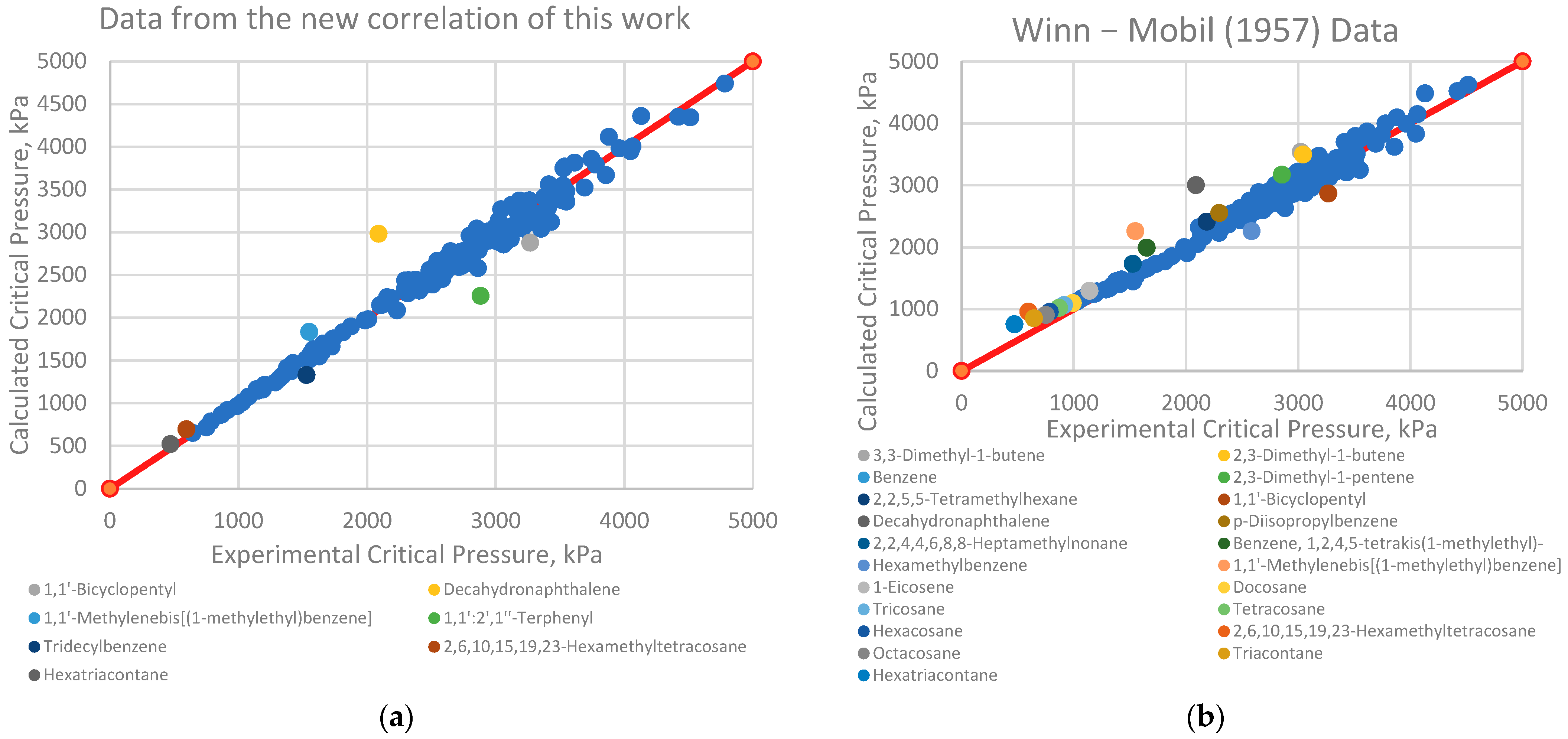
• Critical Pressure Correlation (18): R² = 0.9832.

These high R² values indicate excellent agreement between the predicted and experimental values, demonstrating the robustness of our new empirical models.

Figure 3 illustrates the fitness of the critical temperature predicted by the ANN versus the measured critical temperature. The ANN model demonstrates an exceptionally high accuracy in the prediction of the critical temperature, with R = 0.99913 and a standard error of 4.1 °C.

As indicated in Figure 4, a mean squared error of 0.00010394 was achieved at epoch 4.

Figure 5 shows the fitness of the critical pressure predicted by the ANN versus the measured critical pressure. The ANN model demonstrates an exceptionally high accuracy in the prediction of the critical temperature, with R = 0.99913 and a standard error of 4.1 °C.

Figure 6 indicates that a mean squared error of 0.0019178 was achieved at epoch 10.

All the correlations for critical temperature and pressure estimation detailed in Table 1 use two parameters—most commonly, the normal boiling point (T_b) and specific gravity (SG). In contrast, the correlations and ANN models proposed in this work introduce a third parameter: hydrocarbon molecular weight (M_w). Although the molecular weight can be predicted using T_b and SG, as shown by Stratiev et al. [25], we found that incorporating M_w significantly enhances the accuracy of critical property predictions.

Table 6. Statistical analysis of the studied correlations in predicting the critical temperature of hydrocarbons.

Correlation	Standard Error	Relative Standard Error	Sum of Squared Errors	%AAD	SRE
New empirical correlation (this work)	6.94	1.1	0.0195	0.74%	−4.62
ANN model	4.1	0.66	0.006	0.39%	190.258
Winn–Mobil (1957) [13]	9.74	1.6	0.0359	0.86%	−762.003
Cavett (1962) [11]	9.99	1.6	0.0358	0.99%	−234.396
Lee–Kesler (1976) [10]	7.35	1.2	0.0215	0.74%	−405.665
Riazi–Daubert (1980) [8]	7.69	1.2	0.02341	0.75%	0.64
Riazi (1987) [7]	8.205	1.3	0.0240	0.77%	412.145
Tsonopoulos (1986) [14]	9.53	1.5	0.0312	0.88%	46.36
Twu (1987) [12]	7.55	1.2	0.0212	0.73%	311.856
Lin–Chao (1984) [16]	196.38	31.4	10.063	10.84%	−2896.87
Jianzhong et al. (1998) [17]	7.95	1.3	0.0243	0.77%	392.453
Hosseinifar (2014) from MW [15]	20.84	3.3	0.1599	2.13%	−1016.19
Hosseinifar (2014) from NBP [15]	16.65	2.7	0.0845	1.47%	−673.57

provides a detailed evaluation of the different correlations, along with the new correlation (Equation (18)), and the ANN model for predicting critical temperature, specifically for a selected set of hydrocarbon experimental data.

Figure 7, Figure 8, Figure 9, Figure 10, Figure 11 and Figure 12 present the parity graphs of the predicted versus measured critical temperatures of the 176 hydrocarbons using the following empirical correlations: the new empirical correlation of this work (Figure 7a), the Winn–Mobil (1957) [13] correlation (Figure 7b), the Cavett (1962) [11] correlation (Figure 8a), the correlation of Lee–Kesler (1976) [10] (Figure 8b), the Riazi–Daubert (1980) [8] correlation (Figure 9a), the Riazi (1987) [7] correlation (Figure 9b), the Tsonopoulos (1986) [14] correlation (Figure 10a), the Twu (1987) [12] correlation (Figure 10b), the Lin–Chao (1984) [16] correlation (Figure 11a), the Jianzhong (1998) [17] correlation (Figure 11b), and the Hosseinifar (2014) [15] correlation, where the critical temperature is explicit of molecular weight (Figure 12a) and normal boiling point (Figure 12b).

Table 7. Statistical analysis of the studied correlations in predicting the critical pressure of hydrocarbons.

Correlation	Standard Error	Relative Standard Error	Sum of Squared Errors	%AAD	SRE
New empirical correlation (this work)	138.016	6.8	0.5317	3.39%	0.25
ANN model	91.7	3.44	0.170	2.12%	−1.14
Winn–Mobil (1957)	182.536	6.8	1.879	5.66%	6.62
Cavett (1962)	183.363	7.3	1.611	5.02%	6.51
Lee–Kesler (1976)	160.420	6.0	1.007	4.48%	2.04
Riazi–Daubert (1980)	180.936	6.8	1.524	5.50%	0.64
Riazi (1987)	358.963	13.5	4.095	7.39%	8.06
Tsonopoulos (1986)	210.334	7.9	2.342	6.81%	4.15
Twu (1987)	689.905	25.9	7.904	14.79%	−21.50
Lin–Chao (1984)	104,181.9	3907.6	328,939.3	798.89%	730.10
Jianzhong et al. (1998)	182.262	6.8	2.18	6.08%	6.11
Hosseinifar (2014) from MW	224.501	8.4	1.7616	7.16%	1.39
Hosseinifar (2014) from NBP	338.231	12.7	3.865	9.91%	−1.12

provides the results of the evaluation of the different correlations, along with the new one (Equation (19)) and the ANN model for critical pressure prediction for the selected set of hydrocarbon experimental data.

Figure 13, Figure 14, Figure 15, Figure 16, Figure 17 and Figure 18 present the parity graphs of the predicted versus measured critical pressures of the 176 hydrocarbons using the following empirical correlations: the new empirical correlation of this work (Figure 13a), the Winn–Mobil (1957) [13] correlation (Figure 13b), the Cavett (1962) [11] correlation (Figure 14a), the correlation of Lee–Kesler (1976) [10] (Figure 14b), the Riazi–Daubert (1980) [8] correlation (Figure 15a), the Riazi (1987) [7] correlation (Figure 15b), the Tsonopoulos (1986) [14] correlation (Figure 16a), the Twu (1987) [12] correlation (Figure 16b), the Lin–Chao (1984) [16] correlation (Figure 17a), the Jianzhong (1998) [17] correlation (Figure 17b), and the Hosseinifar (2014) [15] correlation, where the critical temperature is explicit of molecular weight (Figure 18a) and normal boiling point (Figure 18b).

The performance of different correlations in predicting the critical temperature T_c is superior to their performance in predicting the critical pressure P_c. The criterion for a “bad point” in predicting T_c is defined as an error above 20 K, which roughly translates to between 2.19% and 4.42%. For P_c, the criterion for a “bad point” is a deviation of more than 10%.

The numbers of “bad points” from evaluating the critical temperature correlations discussed in this work are as follows:

• New Empirical Correlation (this work): 3;
• ANN model: 1;
• Winn–Mobil (1957) [13]: 10;
• Cavett (1962) [11]: 11;
• Lee–Kesler (1976) [10]: 7;
• Riazi–Daubert (1980) [8]: 4;
• Riazi (1987) [7]: 5;
• Tsonopoulos (1986) [14]: 12;
• Twu (1987) [12]: 4;
• Lin–Chao (1984) [16]: 78;
• Jianzhong et al. (1998) [17]: 5.

The numbers of “bad points” from evaluating the critical pressure correlations discussed in this work are as follows:

• New Empirical Correlation (this work): 7;
• ANN model: 2;
• Winn–Mobil (1957) [13]: 21;
• Cavett (1962) [11]: 18;
• Lee–Kesler (1976) [10]: 13;
• Riazi–Daubert (1980) [8]: 19;
• Riazi (1987) [7]: 28;
• Tsonopoulos (1986) [14]: 27;
• Twu (1987) [12]: 77;
• Lin–Chao (1984) [16]: 76;
• Jianzhong et al. (1998) [17]: 25.

The calculated critical properties using the correlations evaluated here were utilized to perform vapor pressure predictions at each component’s normal boiling point, employing the Soave–Redlich–Kwong (SRK) equation of state [26]. The predicted vapor pressure values were then compared to the calculated value using the database critical temperature and pressure data. The correct result for each data point is 101.325 kPa, representing normal atmospheric pressure. A statistical analysis for each correlation method was calculated based on these vapor pressure predictions. Vapor pressure was calculated using the Soave–Redlich–Kwong (SRK) equation of state [26] and the Lee–Kesler equation of state [27], with original critical properties for comparison purposes. These equations are widely used in thermodynamic modeling, but they also have inherent errors in predicting vapor pressure. The results are summarized in

Table 8. Statistical analysis of the studied correlations in predicting vapor pressure at the normal boiling point for the hydrocarbon components.

Correlation	Standard Error	Relative Standard Error	Sum of Squared Errors	%AAD	SRE
SRK equation with original critical properties	2.33	2.30	0.092	1.21%	0.60
Lee–Kesler equation with original critical properties (for comparison)	1.164	1.15	0.0229	0.61%	−0.21
New empirical correlation (this work)	8.705	8.59	1.284	6.46%	0.74
ANN model	6.93	6.84	0.814	4.25%	−2.54
Winn–Mobil (1957) [13]	16.482	16.27	4.604	8.13%	21.30
Cavett (1962) [11]	14.037	13.85	3.339	9.65%	11.00
Lee–Kesler (1976) [10]	11.144	10.99	2.105	7.22%	10.07
Riazi–Daubert (1980) [8]	9.473	9.35	1.521	6.83%	−6.34
Riazi (1987) [7]	9.532	9.41	1.54	7.06%	−6.01
Tsonopoulos (1986) [14]	9.611	9.49	1.565	7.16%	4.22
Twu (1987) [12]	31.689	31.27	17.019	20.45%	−35.59
Lin–Chao (1984) [16]	10,065.9	9934.3	1,687,593.0	2483.99%	2373.21
Jianzhong et al. (1998) [17]	9.165	9.05	1.4236	7.16%	−1.27
Hosseinifar (2014) from MW [15]	36.318	35.84	22.35	22.54%	25.06
Hosseinifar (2014) from NBP [15]	31.080	30.67	16.371	15.91%	13.19

, which provides a comprehensive statistical analysis of the studied correlations for predicting vapor pressure at normal boiling points for hydrocarbon components.

4. Discussion

As can be seen in ref. [28], taking gasoline as an example, the composition of the different gasoline fractions differs substantially.

• Straight-run naphtha predominantly consists of n-alkanes and iso-alkanes, with up to 10% aromatic compounds.
• Isomerate and alkylate are mostly iso-alkanes with small amounts of n-alkanes.
• FCC-Gasoline contains 20–40% olefins and 20–35% aromatics, with the rest being n-alkanes and iso-alkanes.
• Reformate comprises 60–70% aromatics and 0–2% olefins, with the remainder as normal alkanes, iso-alkanes, and cyclo-alkanes.

These differences in composition also influence thermodynamic properties, like critical temperature (T_c) and critical pressure (P_c), which are crucial for calculating vapor pressure. The complexity of hydrocarbon molecules affects the precision of these calculations. For the critical pressure, the deviation is more noticeable due to the larger and more complex molecules. The components that exhibit noticeable deviations between the predicted and experimental values of the critical pressure are 3,3-dimethyl-1-butene, 2,3-dimethyl-1-butene, cyclohexene, cycloheptane, cyclooctane, indane, 1,1’-bicyclopentyl, decahydronaphthalene, 1,3-dimethyladamantane, tetralin, p-diisopropylbenzene, 1,3,5-triethylbenzene, naphthalene, hexylbenzene, 1-methylnaphthalene, hexamethylbenzene, tricosane, tetracosane, hexacosane, 2,6,10,15,19,23-hexamethyltetracosane, octacosane, triacontane, and hexatriacontane.

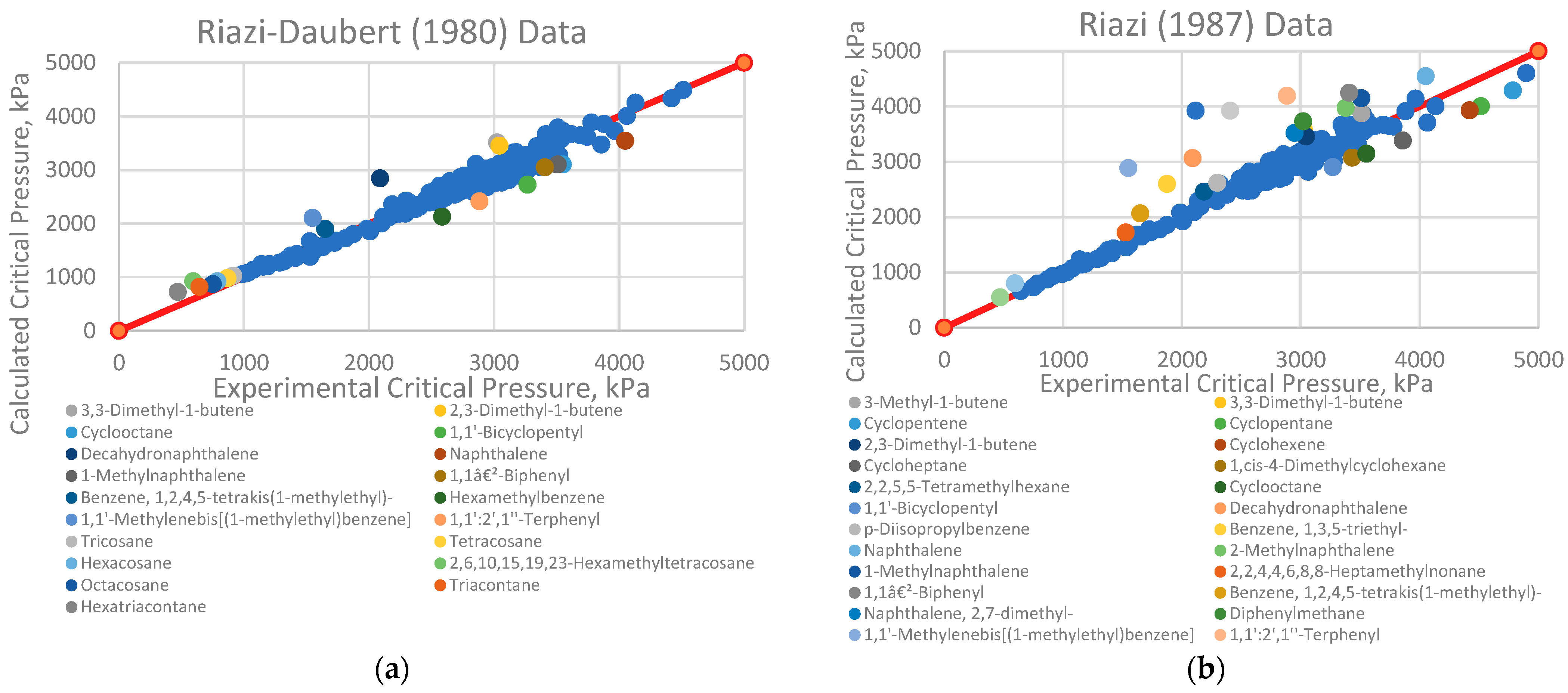
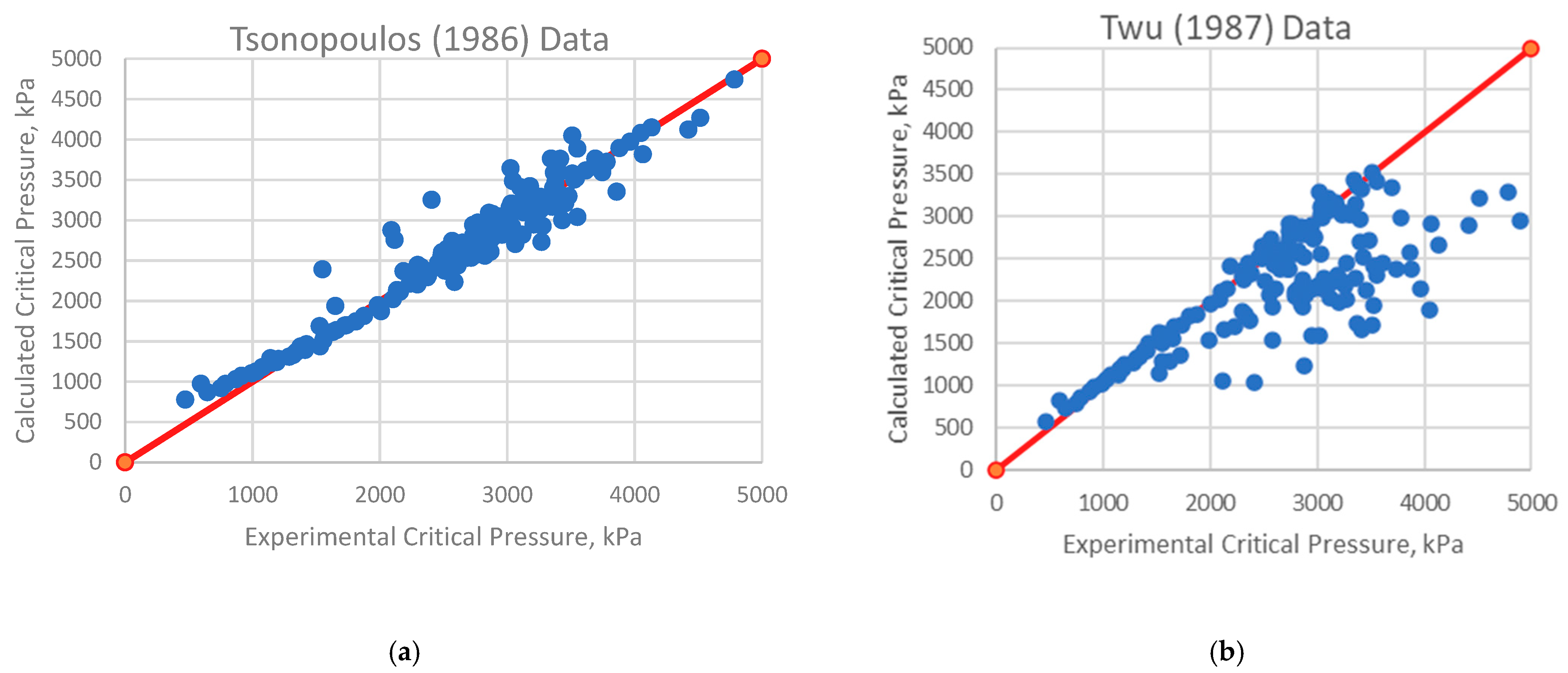
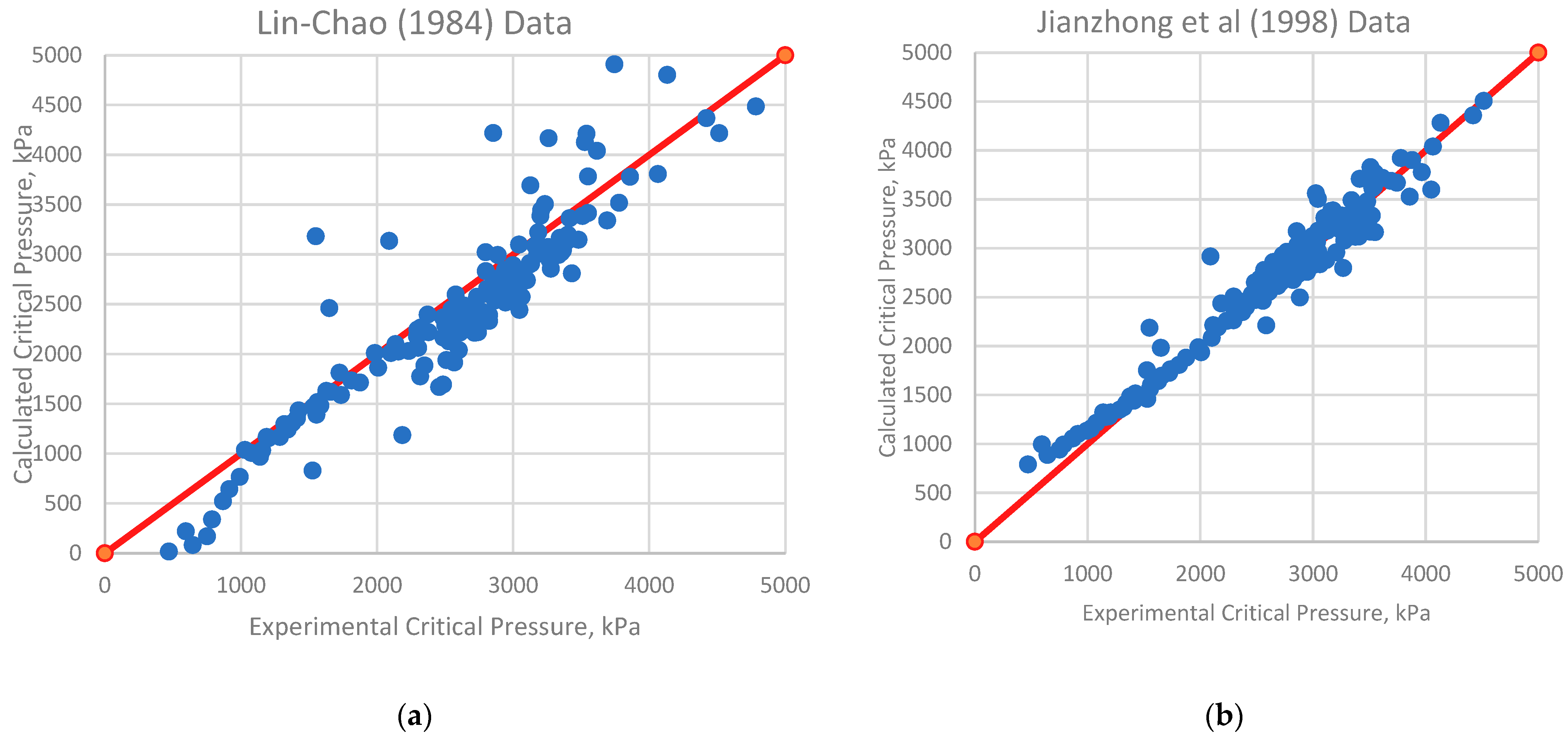
4.1. Analysis of Deviations

These components primarily belong to the following categories:

• Branched alkenes, such as 3,3-dimethyl-1-butene and 2,3-dimethyl-1-butene.
• Cyclo-alkanes/alkenes, including cyclohexene, cycloheptane, and cyclooctane.
• Poly-substituted benzene derivatives, for example, indane, p-diisopropylbenzene, and 1,3,5-triethylbenzene.
• Poly-aromatics, such as naphthalene and 1-methylnaphthalene.
• Polycyclic compounds, including 1,1’-bicyclopentyl, decahydronaphthalene, tetralin, and triacontane.
• Heavy alkanes, like tricosane, tetracosane, hexacosane, and hexatriacontane.

The listed components show the highest deviations in critical pressure prediction. They are predominantly branched alkenes, cyclo-alkanes/alkenes, poly-substituted benzene derivatives, polycyclic compounds, and heavy alkanes.

4.2. Implications for Correlation Performance

No single correlation can address all the issues with critical pressure prediction across the entire range of hydrocarbons. The proposed correlation, while still showing some errors between experimental and calculated values, demonstrates smaller deviations compared to the other correlations discussed in this work. This indicates its potential superiority over the existing methods for predicting critical pressures.

The novelty in the correlations presented in this work is the addition of one more parameter not included in the previous correlations, that is, the molecular weight. The ANN model, in addition to the molecular weight, also employs the acentric factor, which, as observed, further improved the accuracy of critical property calculations. For petroleum fractions and generated pseudo-components, the molecular weight can be calculated with higher precision, as discussed in our previous work [18]. The cause for the bigger deviations in the critical property prediction is the complexity of the molecules of these hydrocarbons—including higher hydrocarbon chain length, branching, the presence of double bonds, and the presence of aromatic rings. The input parameters for the correlations cannot sufficiently address all the influences that the hydrocarbon structure has on the critical properties of the compounds.

4.3. Future Applications

Testing the proposed correlations in more complex simulations of refinery units, especially those involving cracking, reforming, or other complex reactions, would be beneficial. These processes lead to products with diverse compositions and properties, which can further validate the accuracy and robustness of the correlation under challenging conditions.

A good example for testing the new correlation performance would be a process simulation of a naphtha splitter column. Two simulation cases can be performed, and the results can be compared. Since the reformer feed (naphtha) is within the gasoline boiling range, a GC analysis of the available components can be performed. Based on the analysis, a set of 40 to 50 pure components with meaningful concentrations can be identified, and the composition can be normalized. Alternatively, a TBP or ASTM distillation curve analysis may be performed for the products of the reformate splitter column, and pseudo-components may be initialized. The critical properties of these pseudo-components can be calculated using the new correlation methods. The results from both simulations using defined components and pseudo-components, detailing the performance of the naphtha splitter column, can be compared and analyzed. A good pseudo-component generation can closely match the results obtained from more rigorous simulations of individual components.

5. Conclusions

In this study, we conducted a thorough comparison of various methods for predicting the critical temperature (T_c) and critical pressure (P_c) of petroleum fractions and individual hydrocarbons. The previous correlations use the boiling point and specific gravity as input variables. The application of ICrA for evaluating the data of 176 individual hydrocarbons, however, revealed that the molecular weight has a statistically meaningful relation to the critical properties. Indeed, the inclusion of molecular weight in the newly developed correlations turned out to improve the accuracy of critical property calculation. The additional involvement of the acentric factor in the ANN model further improves the precision of critical property computation. The new prediction models of critical properties are in the process of verification for rating the performance of separation equipment in various oil refining units.

References

1. Ambrose, D. Correlation and Estimation of Vapour-Liquid Critical Properties. I. Critical Temperatures of Organic Compounds; NPL Rep. Chem. 92; National Physical Laboratory: Teddington, UK, 1978. [Google Scholar]
2. Lydersen, A.L. Estimation of Critical Properties of Organic Compounds; Eng Exp Sta Report 3; University of Wisconsin: Madison, WI, USA, 1955. [Google Scholar]
3. Nannoolal, Y.; Rarey, J.; Ramjugernath, D. Estimation of Pure Component Properties. Part 2. Estimation of Critical Property Data by Group Contribution. Fluid Phase Equilibria 2007, 252, 1–27. [Google Scholar] [CrossRef]
4. Korsten, H. Critical Properties of Hydrocarbon Systems. Chem. Eng. Technol. 1998, 21, 229–244. [Google Scholar] [CrossRef]
5. Hajipour, S.; Satyro, M.A. Uncertainty Analysis Applied to Thermodynamic Models and Process Design—1. Pure Components. Fluid Phase Equilibria 2011, 307, 78–94. [Google Scholar] [CrossRef]
6. Kumar, A.; Okuno, R. Critical Parameters Optimized for Accurate Phase Behavior Modeling for Heavy N-Alkanes up to C100 Using the Peng–Robinson Equation of State. Fluid Phase Equilibria 2012, 335, 46–59. [Google Scholar] [CrossRef]
7. Riazi, M.R. Characterization and Properties of Petroleum Fractions, 1st ed.; ASTM International: West Conshohocken, PA, USA, 2005; pp. 60–66. [Google Scholar]
8. Riazi, M.R.; Daubert, T.E. Simplify Property Predictions. Hydrocarb. Process. 1980, 59, 115–116. [Google Scholar]
9. The American Petroleum Institute and EPCON International. API Technical Data Book, 10th ed.; EPCON International™: Houston, TX, USA, 2016. [Google Scholar]
10. Kesler, M.G.; Lee, B.I. Improve Prediction of Enthalpy of Fractions. Hydrocarb. Process. 1976, 55, 153–158. [Google Scholar]
11. Cavett, R.H. Physical Data for Distillation Calculations, Vapor-Liquid Equilibria. In Proceedings of the 27th Midyear Meeting, API Division of Refining, San Francisco, CA, USA, 15 May 1962. [Google Scholar]
12. Twu, C.H. An Internally Consistent Correlation for Predicting the Critical Properties and Molecular Weights of Petroleum and Coal-Tar Liquids. Fluid Phase Equilibria 1984, 16, 137–150. [Google Scholar] [CrossRef]
13. Winn, F.W. Physical Properties by Nomogram. Petroleum Refiners. 1957, 36, 157–159. [Google Scholar]
14. Tsonopoulos, C.; Heidman, J.L.; Hwang, S.C. Thermodynamic and Transport Properties of Coal Liquids (Exxon Monographs Series), 1st ed.; John Wiley & Sons: New York, NY, USA, 1986. [Google Scholar]
15. Hosseinifar, P.; Jamshidi, S. Development of a New Generalized Correlation to Characterize Physical Properties of Pure Components and Petroleum Fractions. Fluid Phase Equilibria 2014, 363, 189–198. [Google Scholar] [CrossRef]
16. Lin, H.-M.; Chao, K.-C. Correlation of Critical Properties and Acentric Factor of Hydrocarbons and Derivatives. AIChE J. 1984, 30, 981–983. [Google Scholar] [CrossRef]
17. Zhang, J.; Zhang, B.; Zhao, S.; Wang, R.; Yang, G. Simplified Prediction of Critical Properties of Nonpolar Compounds, Petroleum, and Coal Liquid Fractions. Ind. Eng. Chem. Res. 1998, 37, 2059–2060. [Google Scholar]
18. Atanassov, K.; Mavrov, D.; Atanassova, V. Intercriteria Decision Making: A New Approach for Multicriteria Decision Making, Based on Index Matrices and Intuitionistic Fuzzy Sets. In Issues in Intuitionistic Fuzzy Sets and Generalized Nets, 11; Atanassov, K., Kacprzyk, J., Krawczak, M., Szmidt, E., Eds.; Warsaw School of Information Technology: Warsaw, Poland, 2014; pp. 1–8. [Google Scholar]
19. Atanassov, K.; Atanassova, V.; Gluhchev, G. Intercriteria Analysis: Ideas and Problems. Notes Intuitionistic Fuzzy Sets 2015, 21, 81–88. [Google Scholar]
20. Mavrov, D. Software for InterCriteria Analysis: Implementation of the Main Algorithm. Notes Intuitionistic Fuzzy Sets 2015, 21, 77–86. [Google Scholar]
21. Mavrov, D. Software for Intercriteria Analysis: Working with the Results. Annu. Inform. Sect. Union Sci. Bulg. 2015, 8, 37–44. [Google Scholar]
22. Ikonomov, N.; Vassilev, P.; Roeva, O. ICrAData—Software for InterCriteria Analysis. Int. J. Bioautom. 2018, 22, 1–10. [Google Scholar] [CrossRef]
23. Atanassov, K.; Atanassova, V.; Chountas, P.; Mitkova, M.; Sotirova, E.; Sotirov, S.; Stratiev, D. Intercriteria analysis over normalized data. In Proceedings of the 2016 IEEE 8th International Conference on Intelligent Systems (IS), Sofia, Bulgaria, 4–6 September 2016; pp. 564–566. [Google Scholar]
24. Atanassov, K. On Intuitionistic Fuzzy Sets Theory; Springer: Berlin/Heidelberg, Germany, 2012. [Google Scholar]
25. Stratiev, D.; Sotirov, S.; Sotirova, E.; Nenov, S.; Dinkov, R.; Shishkova, I.; Kolev, I.V.; Yordanov, D.; Vasilev, S.; Atanassov, K.; et al. Prediction of Molecular Weight of Petroleum Fluids by Empirical Correlations and Artificial Neuron Networks. Processes 2023, 11, 426. [Google Scholar] [CrossRef]
26. Soave, G. Equilibrium Constants from a Modified Redlich-Kwong Equation of State. Chem. Eng. Sci. 1972, 27, 1197–1203. [Google Scholar] [CrossRef]
27. Lee, B.I.; Kesler, M.G. A Generalized Thermodynamic Correlation Based on Three-parameter Corresponding States. AIChE J. 1975, 21, 510–527. [Google Scholar] [CrossRef]
28. le Goff, P.Y.; Kostka, W.; Ross, J. Catalytic Reforming. In Springer Handbook of Petroleum Technology (Springer Handbooks), 2nd ed.; Hsu, C.S., Robinson, P.R., Eds.; Springer: Cham, Switzerland, 2017; pp. 589–615. [Google Scholar]
Figure 1. Results oof the ICrA application for critical temperature visualized in the intuitionistic fuzzy interpretational triangle.
Fuels 06 00036 g001
Figure 2. Results of the ICrA application for critical pressure visualized in the intuitionistic fuzzy interpretational triangle.
Fuels 06 00036 g002
Figure 3. ANN-predicted versus experimental critical temperature values for training, validation, testing, and the overall dataset of 176 individual hydrocarbons.
Fuels 06 00036 g003
Figure 4. Neural network training performance for the prediction of critical temperature. The green circle indicates the point where the minimum mean squared error is obtained.
Fuels 06 00036 g004
Figure 5. ANN-predicted versus experimental critical pressure values for training, validation, testing, and the overall dataset of 176 individual hydrocarbons.
Fuels 06 00036 g005
Figure 6. Neural network training performance for the prediction of critical pressure. The green circle indicates the point where the minimum mean squared error is obtained.
Fuels 06 00036 g006
Figure 7. Parity graph displaying the experimental critical temperature data versus the calculated data performed by the new correlation Equation (18) (a) and the Winn–Mobil (1957) [13] correlation Equation (1) (b). The components displayed below each graph are the ones that have more than 20 K error between the calculated and experimental critical temperatures.
Fuels 06 00036 g007
Figure 8. Parity graph displaying the experimental critical temperature data versus the calculated data performed by the Cavett (1962) [11] correlation Equation (2) (a) and the Lee–Kesler (1976) [10] correlation Equation (3) (b). The components displayed below each graph are the ones that have more than 20 K error between the calculated and experimental critical temperatures.
Fuels 06 00036 g008
Figure 9. Parity graph displaying the experimental critical temperature data versus the calculated data performed by the Riazi–Daubert (1980) [8] correlation Equation (4) (a) and the Riazi (1987) [7] correlation Equation (5) (b). The components displayed below each graph are the ones that have more than 20 K error between the calculated and experimental critical temperatures.
Fuels 06 00036 g009
Figure 10. Parity graph displaying the experimental critical temperature data versus the calculated data performed by the Tsonopoulos (1986) [14] correlation Equation (6) (a) and the Twu (1987 [12]) correlation Equation (7) (b). The components displayed below each graph are the ones that have more than 20 K error between the calculated and experimental critical temperatures.
Fuels 06 00036 g010
Figure 11. Parity graph displaying the experimental critical temperature data versus the calculated data performed by the Lin–Chao (1984) [16] correlation Equation (8) (a) and the Jianzhong (1998) [17] correlation Equation (9) (b). The components displayed below each graph are the ones that have more than 20 K error (Jianzhong) and 50K (Lin–Chao) between the calculated and experimental critical temperatures.
Fuels 06 00036 g011
Figure 12. Parity graph displaying the experimental critical temperature data versus the calculated data performed by the Hosseinifar (2014) [15] correlation explicit of molecular weight (a) and the Hosseinifar (2014) [15] correlation explicit of normal boiling point Equation (10) (b). The components displayed below each graph are the ones that have more than 20 K error between the calculated and experimental critical temperatures.
Fuels 06 00036 g012
Figure 13. Parity graph displaying the experimental critical pressure data versus the calculated data performed by the new correlation Equation (18) proposed in this work (a) and the Winn–Mobil (1957) [13] correlation Equation (1) (b). The components displayed below each graph are the ones that have more than 10% error between the calculated and experimental critical pressures.
Fuels 06 00036 g013
Figure 14. Parity graph displaying the experimental critical pressure data versus the calculated data performed by the Cavett (1962) [11] Equation (2) (a) and the Lee–Kesler (1976) [10] correlation Equation (3) (b). The components displayed below each graph are the ones that have more than 10% error between the calculated and experimental critical pressures.
Fuels 06 00036 g014
Figure 15. Parity graph displaying the experimental critical pressure data versus the calculated data performed by the Riazi–Daubert (1980) [8] Equation (4) (a) and the Riazi (1987) [7] correlation Equation (5) (b). The components displayed below each graph are the ones that have more than 10% error between the calculated and experimental critical pressures.
Fuels 06 00036 g015
Figure 16. Parity graph displaying the experimental critical pressure data versus the calculated data performed by the Tsonopoulos (1986) [14] Equation (6) (a) and the Twu (1987) [12] correlation Equation (7) (b). No components are displayed because too many points have more than 10% error between the calculated and experimental critical pressures.
Fuels 06 00036 g016
Figure 17. Parity graph displaying the experimental critical pressure data versus the calculated data performed by the Lin–Chao (1984) [16] Equation (8) (a) and the Jianzhong (1998) [17] correlation Equation (9) (b). No components are displayed because too many points have more than 10% error between the calculated and experimental critical pressures.
Fuels 06 00036 g017
Figure 18. Parity graph displaying the experimental critical pressure data versus the calculated data performed by the Hosseinifar (2014) [15] Equation (10) explicit of the molecular weight (a) and explicit of the normal boiling point (b). No components are displayed because too many points have more than 10% error between the calculated and experimental critical pressures.
Fuels 06 00036 g018