Article

Elemental Mapping and Characterization of Petroleum-Rich Rock Samples by Laser-Induced Breakdown Spectroscopy (LIBS)

by
Charles Derrick Quarles, Jr.
1,*,
Toni Miao
2,
Laura Poirier
2,
Jhanis Jose Gonzalez
3 and
Francisco Lopez-Linares
2,*
1
Elemental Scientific, 7277 World Communications Drive, Omaha, NE 68122, USA
2
Chevron Technology Center, 100 Chevron Way, Richmond, CA 94801, USA
3
Applied Spectra, Inc., 950 Riverside Pkwy Suite 90, West Sacramento, CA 95605, USA
*
Authors to whom correspondence should be addressed.
Fuels 2022, 3(2), 353-364; https://doi.org/10.3390/fuels3020022
Submission received: 26 April 2022 / Revised: 30 May 2022 / Accepted: 1 June 2022 / Published: 8 June 2022

Abstract

:
The application of Laser-Induced Breakdown Spectroscopy (LIBS) is presented for the direct elemental analysis of hydrocarbon-rich solids. In recent years, LIBS has become a powerful tool for obtaining elemental information and mapping analysis of different petroleum-rich samples with minimal to no sample preparation and without the need to separate the organic matter from the inorganic matter. By selecting the most intense and representative lines, the element distribution in a 2D map can be accessed in less than ten hours. For this reason, two types of hydrocarbon-rich solids were chosen for examination, i.e., core and shale. Nineteen elements were identified in the samples, and 2D mapping for Ca, Mg, Fe, Ti, Ni, C, H, K, O, and S is presented here. A detailed distribution of the elements, and the main components of the hydrocarbons present in these samples, were determined using LIBS. The H/C molar ratio was determined by building H and C calibration curves using data obtained from classical elemental analysis via combustion. These calibration curves contained a high degree of linearity (R2 > 0.98) with the limits of detection for C (193 nm), C (247 nm), and H (656 nm) of 848 mg kg−1, 353 mg kg−1, and 3.5 mg kg−1, respectively. By combining all of this information, LIBS allowed us to determine how these elements were spatially distributed, which elements were dominant in a given sample, and how much hydrocarbon was present, as well as providing a quantitative determination of the H/C molar ratio, and its correlation with the source of origin.

Graphical Abstract

1. Introduction

Ongoing global energy consumption has led to the exploitation of unconventional sources as alternative means of fulfilling high energy demands. Energy supply companies rely heavily on geological information from hydrocarbon-rich rock samples, such as core, shale, and organic-rich sediments, to predict and understand specific oil and gas reserves [1].
Core analysis has implications for reservoir evaluation, in areas including the evaluation of reserves, development, drilling campaigns, production scenarios, and the interpretation of real tests, among others. Core information commonly contains detailed mineralogy information, the definition of the heterogeneity of the reservoir rock, capillary pressure data which defines fluid distribution in the reservoir rock system, and the multiphase fluid flow properties of the reservoir rock. As a result, core data becomes an indispensable resource in the collection of primary reservoir data directed toward the ultimate evaluation of recoverable hydrocarbons in the reservoir [2]. This information varies from field to field and during the lifetime of the field [2,3]. Rock samples, which result from core sampling, reveal many details regarding the history and formation of wells and reserves. As the only direct evidence available from beneath the earth, these are essential components in the assessment of the fundamental geological properties of hydrocarbon reserves [2,3,4]. This information allows geoscientists and reservoir engineers to ascertain the characteristics of the reservoir under consideration. These samples contain information regarding hydrocarbon nature, porosity, grain size, and mineralogy; these are all essential factors that can influence decisions about future drilling locations. Shale gas rocks are also valuable because they are typically characterized by organic matter and a substantial amount of gas that could be technically recoverable. Shale gas resources have become an alternative energy source, particularly in North America, where vast reserves are available [5].
Different analytical protocols are needed to analyze details about hydrocarbon-rich rock samples, such as core and shale [6]. In conventional analyses, hydrocarbon and minerals need to be separated before analysis. Typically, the organic-rich part needs to be extracted from the solid matrix by various standard protocols, which can be lengthy. After this process, the samples must be dried before analysis can occur. These dried samples are then characterized using different surface techniques, depending on the business needs [6]. The mineral part then can be analyzed by X-ray fluorescence (XRF), X-ray diffraction (XRD), Fourier transformed infrared spectroscopy (FTIR), instrumental neutron activation analysis (INAA), and plasma techniques, such as inductively coupled plasma-optical emission spectrometry (ICP-OES) and inductively coupled plasma mass spectrometry (ICP-MS), to determine mineralogy as well as the elemental composition of the samples, respectively [4,6]. A discussion of the pros and cons of utilizing these techniques lies beyond the scope of this article. However, in most cases, the extensive sample preparation steps, the availability of enough samples, or the lack of performance analysis directly in the field, should be considered.
The possibility of having, simultaneously, qualitative/quantitative elemental composition information for hydrocarbon components such as C, H, N, S, and the metals present in the mineral part, with minimum or no sample preparation, would be ideal. Laser-based technologies such as laser ablation inductively coupled plasma mass spectrometry (LA-ICP-MS) or laser-induced breakdown spectroscopy (LIBS) have been used for direct sampling and analysis of shale [7,8], shale rocks [9], and drillcore [10], in addition to their geochemical applications [11,12,13,14,15]. LIBS is a fast analytical technique that can provide lateral and in-depth elemental information about a given sample. A pulsed laser is focused on the sample’s surface to create a microplasma. During the formation of this plasma, electrons of atoms and ions are excited to higher electronic states and then return to their ground state, with the emission of light characteristic of the elements in the sample. The emission intensity of UV, visible, and near IR light (200–900 nm) is proportional to the concentration of the emitting species. Therefore, information on the elemental composition of a given sample can be obtained promptly [16]. LIBS can gather elemental information for all of the elements in the periodic table, making it an appealing technique for determining the elemental composition of the organic matter and the minerals present in core and shale samples. The application of LIBS in 1D for direct determination of the H/C molar ratios of kerogen present on shale and mudrocks, without sample demineralization, was demonstrated to be quick and efficient. This information helps determine the quality of hydrocarbons associated with the reservoir [8].
Determination of the elemental composition of shale rocks by LIBS has recently been demonstrated. Five primary elements (Al, Ca, Si, Mg, and Ti) and carbon were analyzed and quantified. The authors found that the predicted values produced by LIBS were in agreement with those obtained by ICP-OES and a carbon analyzer [9]. Both research groups demonstrated that, as an analytical tool that can analyze such samples with little to no sample preparation, LIBS offers some significant advantages regarding time, cost, and safety. No acid digestion or organic solvent was needed to extract the organic matter. LIBS has also been used to investigate Marcellus shale samples of different depths. The authors showed that LIBS data collected on these shale samples compared reasonably with conventional techniques such as XRF, total organic carbon (TOC), and CHN analyzers [17].
In this work, an evaluation of LIBS for 2D-elemental mapping was performed using two types of hydrocarbon-rich solids: core and shale samples. High-resolution elemental images were produced without any sample preparation, and were used to investigate the 2D distributions of critical elements in the core and shale samples. The hydrogen/carbon molar ratio (H/C) was investigated to determine whether this is a suitable technique for assessing which types of organic matter are present. In addition, the C 193 nm and C 247 nm lines were compared to determine the most suitable atomic line for this type of application. Data collected from LIBS were used to produce high-resolution images for various elements without sample manipulation.

2. Methods

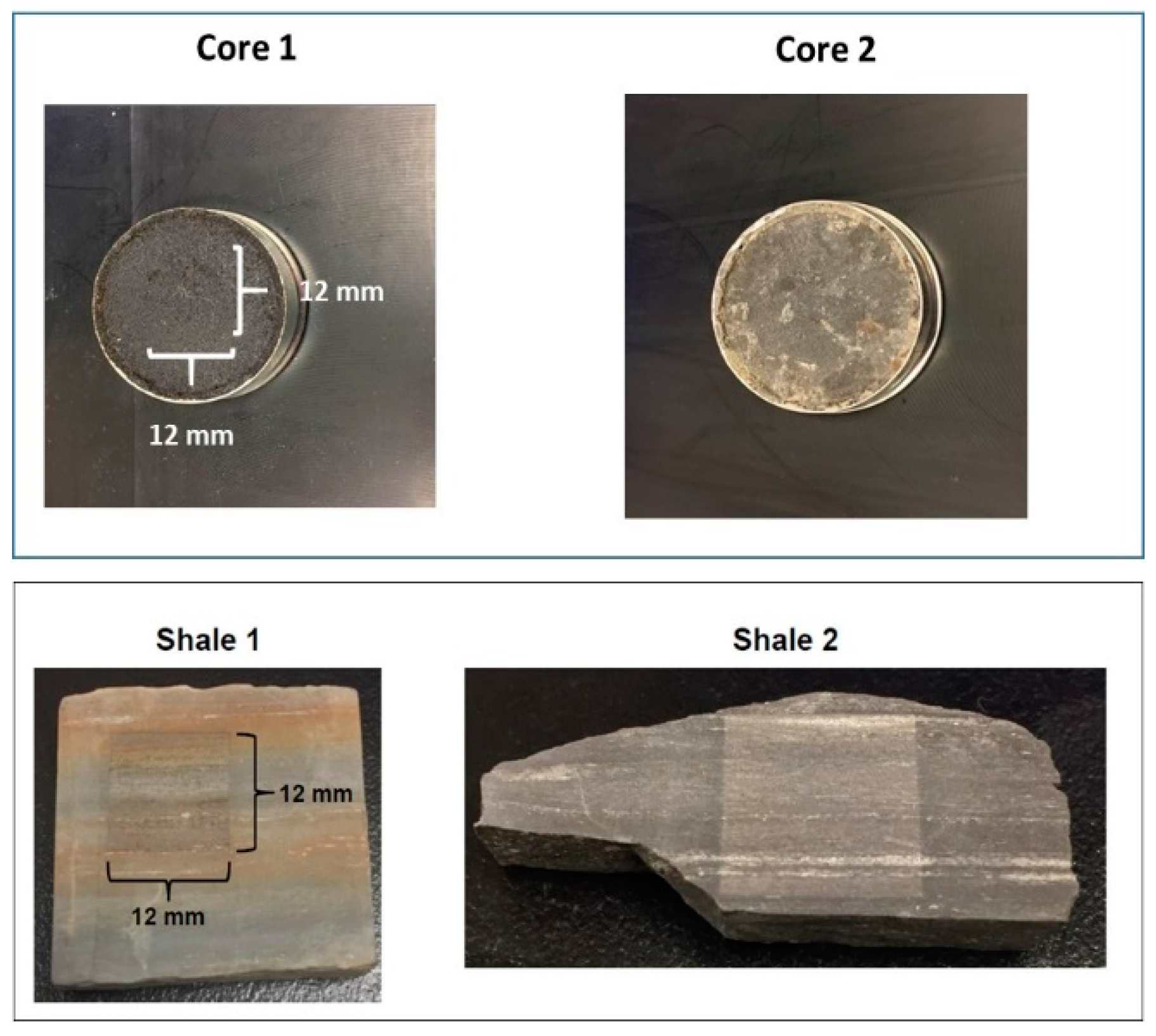
2.1. Samples and Preparation

The Chevron Technology Center (Richmond, CA, USA) provided hydrocarbon-rich solids samples, such as core and shale, from North America. The core samples were pressed into standard 31 mm pellets using a 3630X-press from SPEX (Metuchen, NJ, USA). The shale samples were cut into pieces that ranged from 20–60 mm laterally and were <10 mm in depth.

2.2. Instrumentation

Samples were analyzed using a J200 LIBS tandem instrument (Applied Spectra, Inc., Sacramento, CA, USA). The J200 instrument is equipped with a 266 nm Nd: YAG laser (nanosecond), a six-channel CCD broadband spectrometer with a spectral window of 185–1050 nm, and a gas-purged sample chamber. Full spectra were collected for each laser pulse. However, the selected wavelengths for the elements of interest were: C 193.1 nm, C 247.9 nm, H 656.3 nm, Ca 393.4 nm, Mg 279.6 nm, Ni 361.9 nm, Na 589.6 nm, Li 670.8 nm, Al 394.4 nm, Fe 274.9 nm, Mn 403.5 nm, Si 288.2 nm, Ti 334.9 nm, Be 313.0 nm, Ba 455.4 nm, Sr 407.8 nm, K 766.5 nm, O 777.4 nm, S 921.3 nm, and Rb 780.0 nm. The system is fully integrated and controlled using Applied Spectra’s Axiom 2.0 operation software. The method conditions for both the calibration and mapping methods are listed in Table 1.
The experimental settings were carefully evaluated to obtain the best analytical performance on these samples, and the maximum signal was obtained for each element to minimize shot noise. Additionally, the instrumental conditions displayed in Table 1 enable the best shot-to-shot repeatability and provide the maximum possible signal-to-noise ratio to maximize the dynamic range of the analysis [18].
Ultra-high-purity helium gas (Airgas., Concorde, CA, USA) was used for all experiments to purge any atmospheric gases in the sample chamber. The data (spectra, calibration curves, and elemental maps) were analyzed using Applied Spectra’s data analysis software, Aurora.
Elemental analyses (CHN) were carried out for these samples using a Thermo Scientific™ FLASH 2000 CHNS/O (Thermo Fisher Scientific, Waltham, MA, USA).

2.3. Calibration Standards Preparation

The calibration curves were obtained using Core 1, Core 2, Shale 1, and Shale 2, with hydrogen and carbon contents in ranges of 0.26–1.44 wt.% H, and 2.03–10.1 wt.% C, to cover the expected concentration of these elements. Two of the shale samples that displayed the most visible differences in mineralogy or hydrocarbon content were chosen for elemental mapping.

3. Results and Discussion

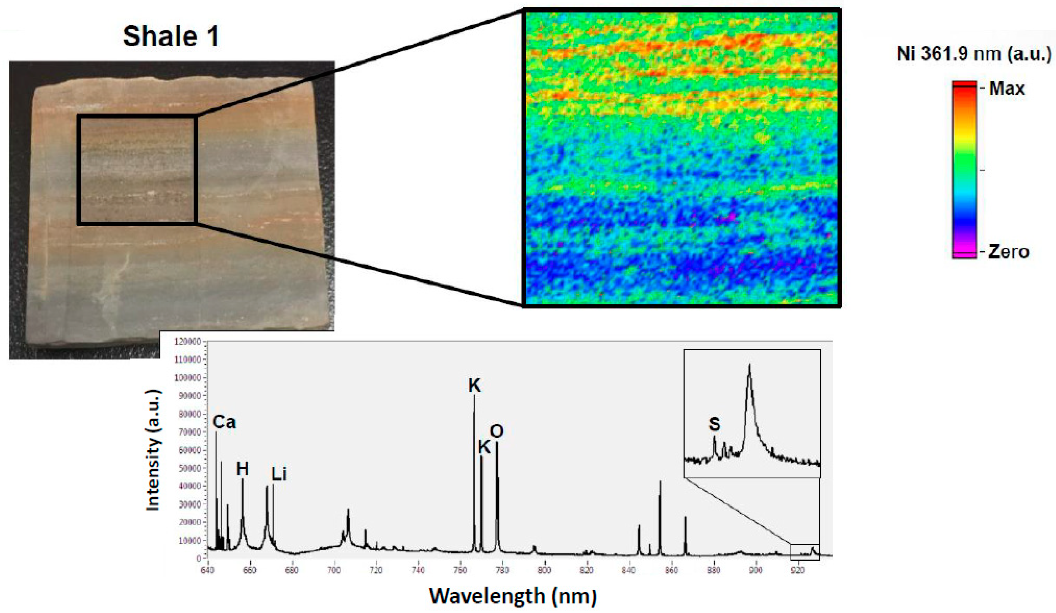
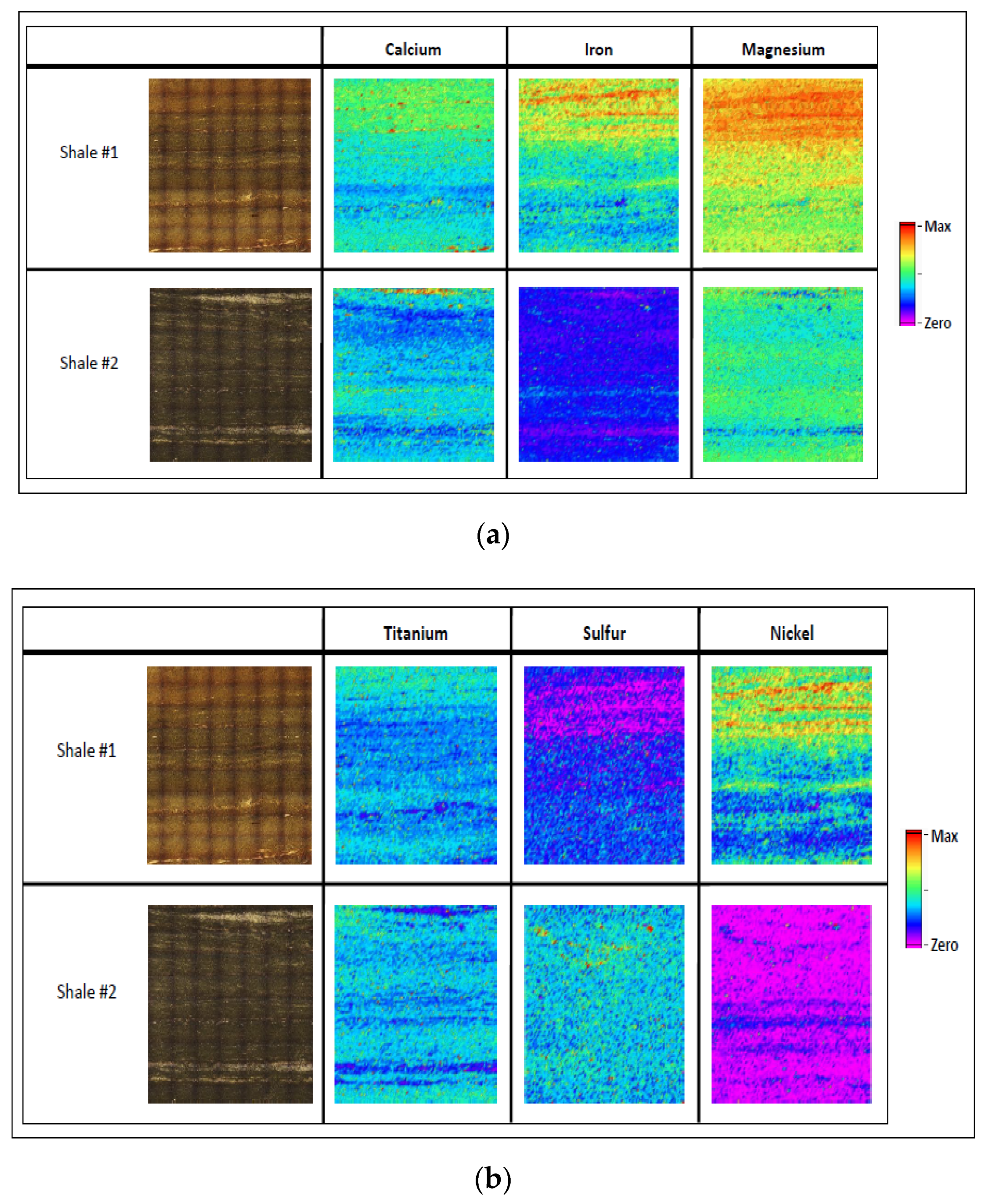
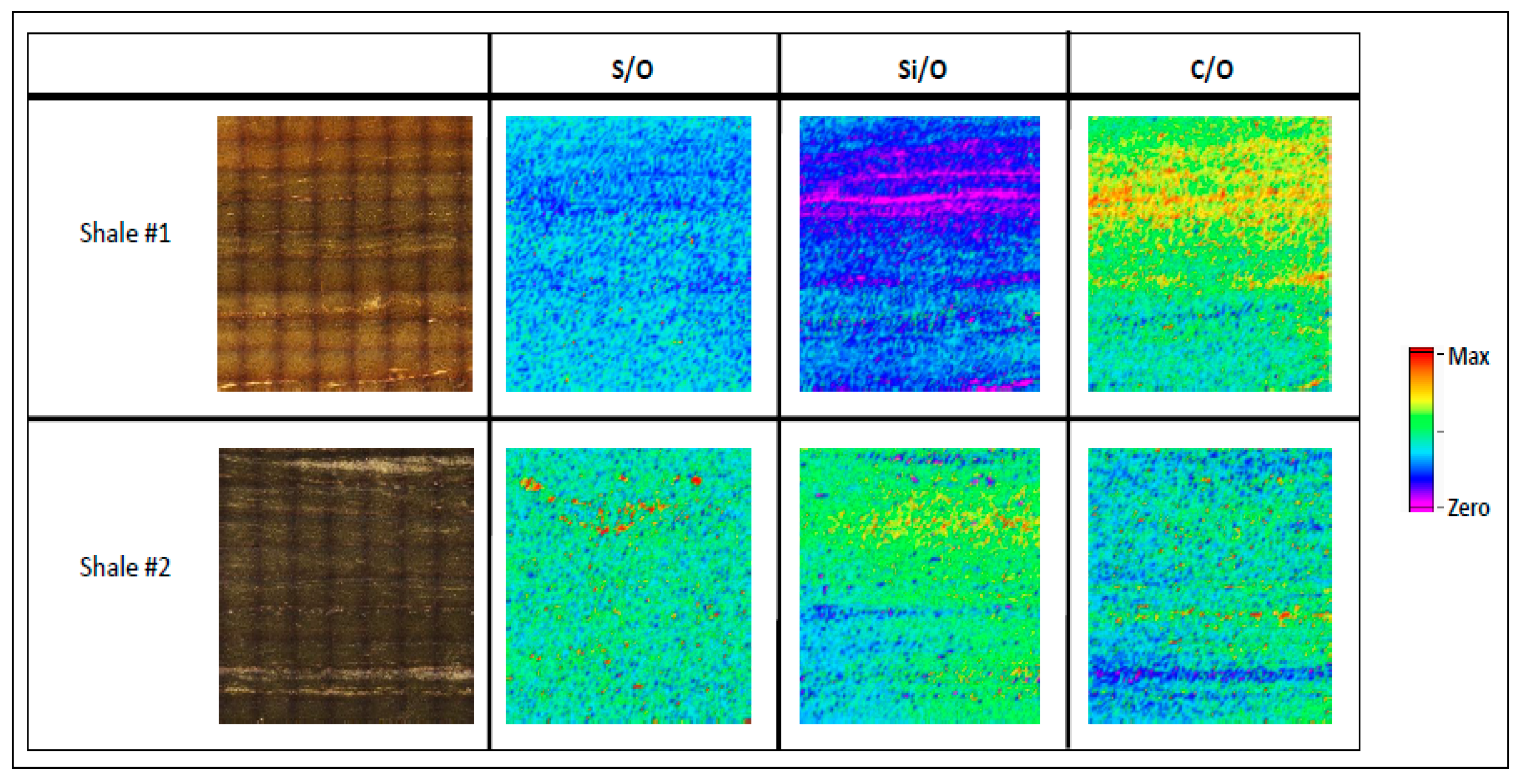
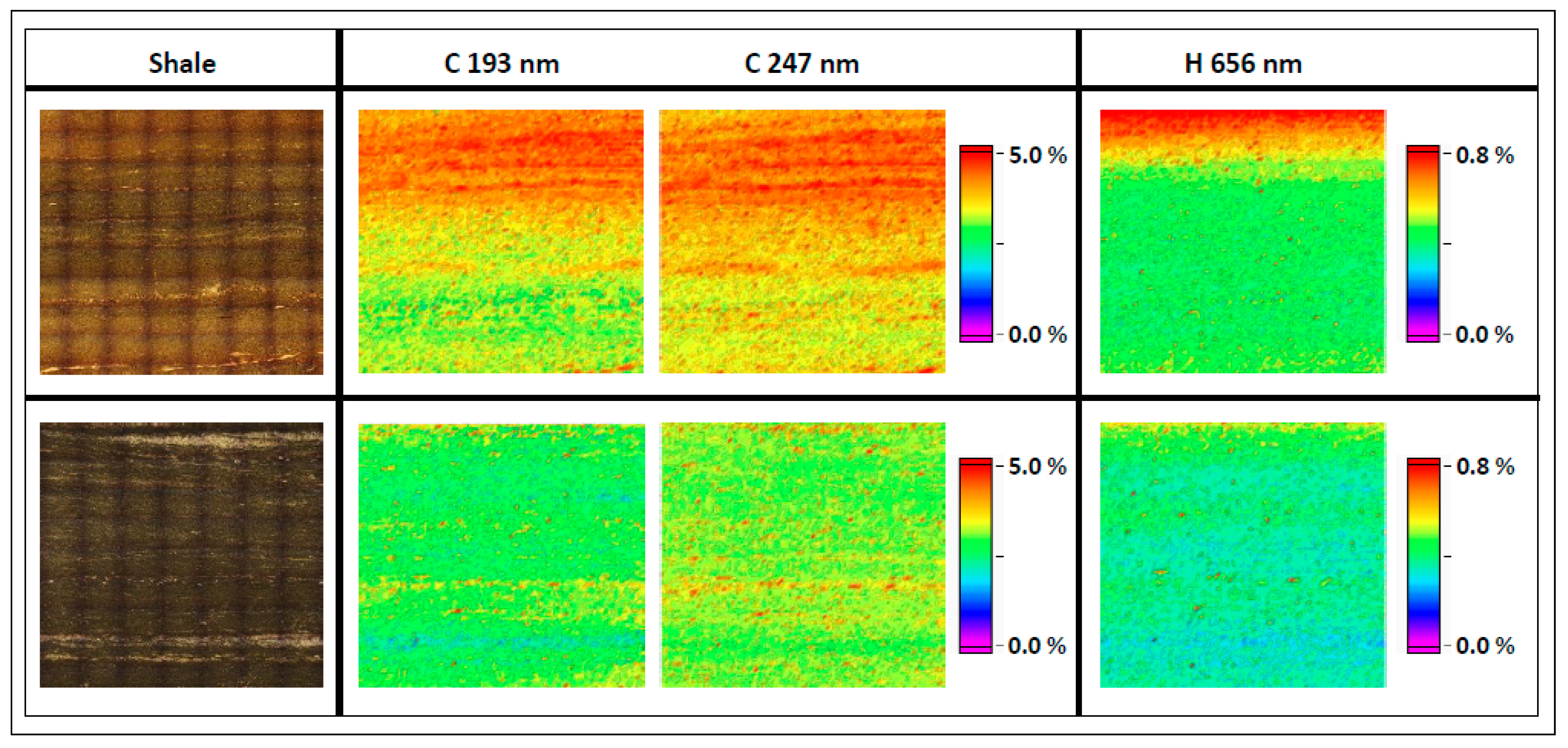
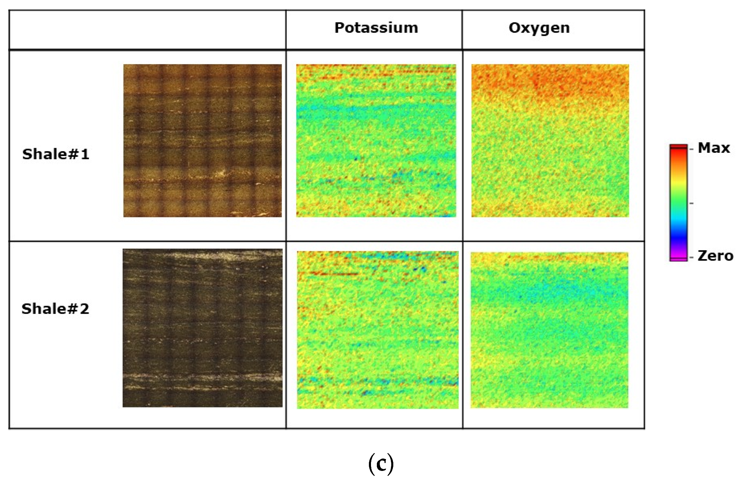
3.1. Elemental Mapping for Hydrocarbon Rich Samples

Initial visual inspection of these samples confirms the heterogeneity present, as expected. The core samples may have variable hydrocarbon content, whereas, in the case of the shale, it is clear that both samples contain layered structures, which differ among the samples. A large 12 mm × 12 mm area was selected to investigate the variation of the elemental composition, as shown in Figure 1.
Figure 1. Hydrocarbon-rich samples were used for LIBS analysis. All samples have different prominent characteristics in mineral and hydrocarbon content, and are suitable for this study. Each laser pulse that ablates the sample over this 144 mm2 area has a unique spectrum per a single location. These spectra can be used to reconstruct spatially selective chemical maps of these samples. Figure 2 shows a portion of a typical LIBS spectrum (displaying 640–940 nm for visual purposes) and a spatially selective chemical map for nickel in shale sample 1.
Fuels 03 00022 g001
Note that small amounts of material are separated at the laser focus point during the ablation process, which creates a small crater after the emission of light [19]. The amount of removed material depends on different factors, such as the type of laser source (ns, fs), the type of material, fluence, absorption of the laser radiation and the heat conduction within the target, the evaporation of material from the target surface, the cooling of the target surface by the heat of evaporation, and the partial absorption of the incident laser beam in the evaporated material [19,20].
The same methodology was applied to all samples. Each spectrum results from accumulating five laser pulses from each single location for an improved signal-to-noise ratio, ensuring that the measurements include some depth information and not the surface alone. The atomic line for a given element (e.g., Ni 361.9 nm) is integrated and then reconstructed into a 2-D image using the x–y coordinates from the laser ablation method. From the initial five laser pulses, a broad set of elements were present in the samples, such as H, Ca, Mg, Ni, Na, Li, Al, Fe, Mn, Si, Ti, Be, Ba, Sr, K, O, S, and Rb. Considering that the objective of this work is to produce a rapid assessment of sample composition and its variability across the surface (2D approach), it is essential to understand the composition of the inorganic components present (minerals, rocks, clays), and the nature of the hydrocarbon present. Elemental maps for C, H, Ca, Mg, Ni, Al, Fe, Ti, K, O, and S are presented in the main manuscript, while the other elements can be seen in the Supplementary Materials.
Figure 3 displays the composition maps for C, H, Si, and Al for core and shale. An initial assessment of the information gathered by elemental mapping indicates the high diversity of the samples and how the elements are distributed accordingly. The distributions of C and H vary depending on the samples; it can be seen that core sample 1 is enriched with C compared to the rest of the samples, and it is well distributed across the entire surface. H follows the same trend, and is more clearly pronounced for core sample 1 and shale sample 1.
Additionally, it can be seen that Si and Al, which are associated with the mineral phase, are the dominant elements in these samples. From Figure 3, we can see how the mapping information can tell us which elements are dominant in the sample. Interestingly, the core 1 sample has a silicon base material, whereas core 2 contains Si and Al homogeneously distributed across the evaluated area.
The shale samples have a visible layer, and the mapping reflects this. As shown in Figure 3, Si and Al are distributed more as a layer than they were in the core sample. The signal intensity illustrates the areas where these elements are abundant. In Figure 3, we can see the power of 2D mapping for the initial inspection and differentiation of these types of materials.
Figure 4a–c display Ca, Fe, Mg, Ti, S, Ni, K, and O for the two shale samples. The maximum intensity for each element differs, but the two shale samples are normalized to each other for the purposes of direct comparison. For both shale samples, the elemental maps correlate nicely to the digital image of the shale area analyzed. The most significant differences between shale sample 1 and shale sample 2 are seen for S, Fe, Ni, and O by visual comparisons. The other elements (Ca, Ti, Al, S, K, and Mg) show subtle differences between the shale samples.
Knowing information about the chemical makeup of a sample can be very useful for understanding what chemical form the element is in (e.g., sulfate (-SO42−), carbonate (-CO32−), or silicate (-SiO44−)). LIBS is a total elemental technique that does not offer chemical compound information; however, examining how the ratio of elements changes from layer to layer can provide some insight. Figure 5 displays the S/O, Si/O, and C/O maps comparing the two shale samples.
The response for S/O is slightly higher in shale sample 2 than in shale sample 1. Additionally, shale sample 2 displays small, localized areas of high S to O responses. For Si/O and C/O, this figure shows transparent layer-to-layer transitions for both shale samples. Shale sample 1 has more carbon than shale sample 2, which appears to be made up of more Si-containing compounds.

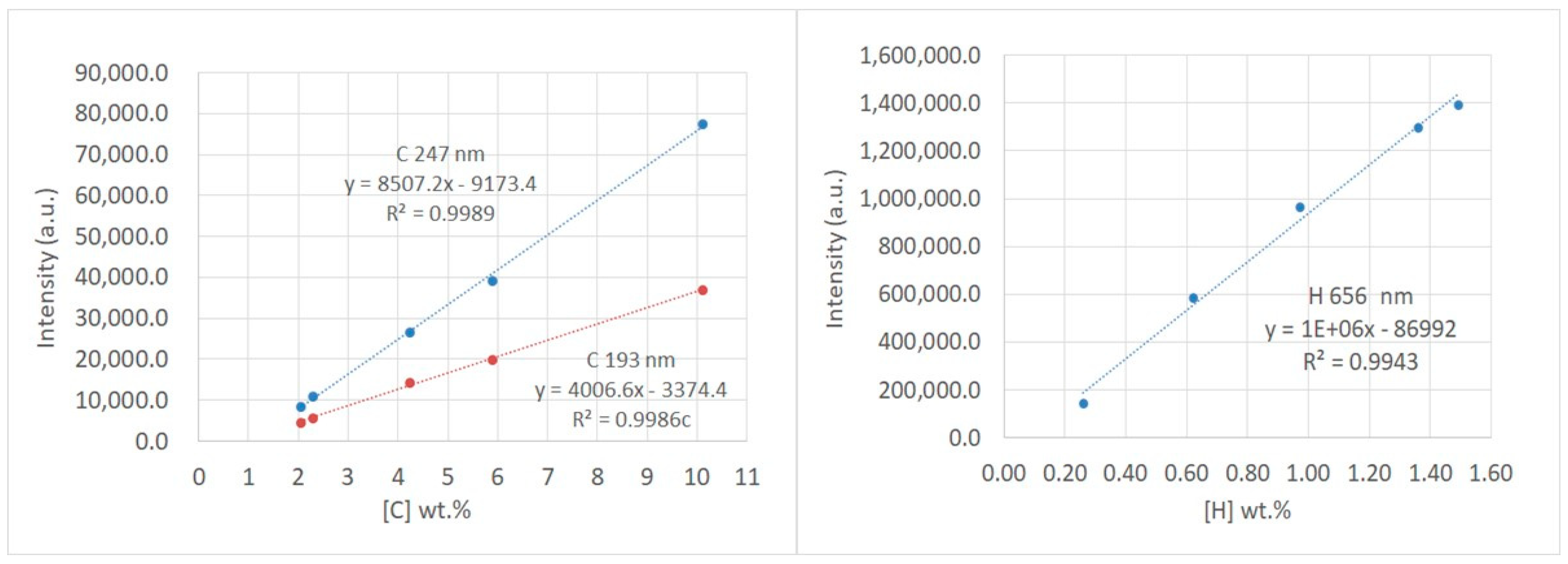
3.2. Calibration Method—Core and Shale

Determining the type of hydrocarbons associated with the core and shale samples regarding the elemental composition is important because it can provide an initial idea of the quality of the petroleum. The H/C molar ratio is useful because it can provide the paraffin/aromatic nature of hydrocarbons associated with the core and shale samples. Additionally, if the core or shale samples have H/C > 1.2, it may indicate that more oil will be obtained from that reservoir, whereas if H/C < 1.2, more gas may be associated with the formation [9]. A quantitative method was developed using two new shale samples and four core samples to create calibration curves for C and H. Since there are no available standard reference materials for shale, a set was created from materials analyzed by independent methods.
The six available samples were analyzed using elemental analysis (CHN) to determine the reference concentrations for the LIBS calibration curves. The most intense atomic line to use for carbon is 247.86 nm, but this line is susceptible to interference. Therefore, the second most intense line, at 193.09 nm, was also monitored. The most intense atomic line for H is found at 656.29 nm. It does not have any interferences that affect the H response (a more sensitive detector would be required to look at the next available and much weaker atomic line). Figure 6 displays the calibration curves for C and H; both show a high correlation to the reference data.
LIBS calibration curves showed good linearity with R2 > 0.98 for all lines. Based on these calibration standards, the limits of detection for C 193 nm, C 247 nm, and H 656 nm were calculated to be 848 mg kg−1, 353 mg kg−1, and 3.5 mg kg−1, respectively. All detection limits are low enough for quantitative analysis of these samples.
A section of each of the two shale samples that best represented the multiple layers analyzed by LIBS was removed and analyzed by CHN elemental analysis to determine method accuracy. Table 2 shows the accuracy of the LIBS method as compared to the reference values.
The accuracy for carbon using the 193 nm atomic line was excellent, showing only a slight negative bias (≤−2.5%). At the same time, the accuracy for carbon using the 247 nm atomic line showed a more significant bias, which is most likely due to interferences from Fe. Some level of bias is to be expected, as the reference value is the total amount of the sample. In contrast, the LIBS values represent spatial information from various layers of the shale sample. Based on these findings, 193 nm is the most appropriate atomic line for quantifying carbon in these samples. However, the 247 nm line will still be presented in subsequent sections to determine how this interference could affect the results of the H/C molar ratios.
The C and H intensity maps were converted to concentration maps using the calibration curves. Figure 7 displays the C 193 nm, C 247 nm, and H 656 nm concentration maps for both shale samples. The map for carbon at 247 nm shows a higher visual amount of carbon, which is expected based on the higher bias seen in Table 2. For shale sample 1, higher amounts of carbon and hydrogen are found in the top layers, whereas for shale sample 2, these elements are more evenly distributed. The two shale samples ranged from ~1.0–5.0 wt.% carbon and ~0.3–0.8 wt.% hydrogen.

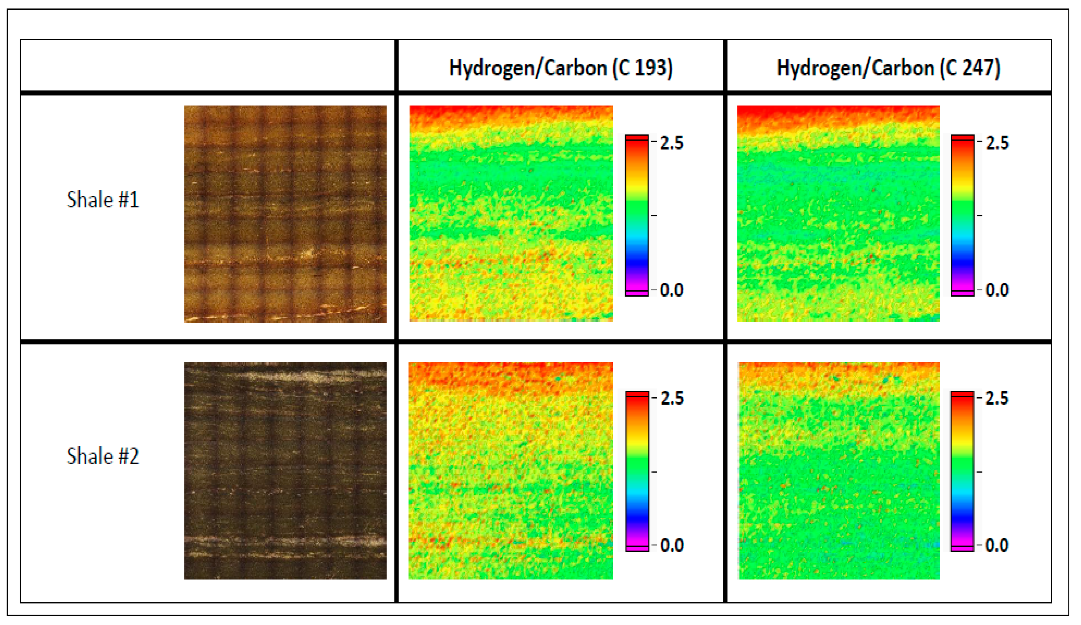
3.3. H/C Molar Ratio Mapping—Shale

This study aims to determine the types of hydrocarbons present in the shale samples, regarding group types such as aliphatic, aromatic, or oxygenate, while simultaneously collecting as much elemental information about the sample as possible.
The following equation was used to convert the concentration values into H/C molar ratios: H/C = (H wt.%/1.00011)/(C wt.%/12.011). Figure 8 shows the hydrogen/carbon ratios for C 193 nm and C 247 nm. For visual purposes, the scale was set from 0–2.5 H/C. Table 3 lists the average H/C values determined for each shale sample. The average H/C values were 1.60 and 1.69 for shale samples 1 and 2, respectively. If the C 247 nm line were used, the H/C would be ~0.08–0.20 lower than the C 193 nm line.
An H/C molar ratio <1 indicates that the hydrocarbon present in the shale sample has a more aromatic nature, whereas an H/C molar ratio >1 indicates that the hydrocarbon is more paraffinic. In this case, the hydrocarbon associated with these samples has a more paraffinic character. This information provides a first approximation of the quality of the hydrocarbon associated with this formation, which could indicate the quantity of hydrogen required to transform the hydrocarbon into valuable products during the refining process [21]. The minimum and maximum H/C molar ratios were calculated to determine how much variation there was in the 12 × 12 mm area. Using the 193 nm carbon data, it can be seen that the hydrocarbon present in such samples is more aliphatic in both cases. Additionally, these values indicate that these reservoirs would be prone to produce more petroleum than gas.
The possibility of obtaining more detailed information about functional groups associated with the hydrocarbon was initially investigated using FTIR microscopy. Preliminary results indicate that FTIR data can complement C/O, and H/C molar ratio, among others, to characterize the functionalities present in the mineral and a hydrocarbon. These results will be presented in future work.

4. Conclusions

The present work illustrates that LIBS is a powerful tool for obtaining 2D elemental mapping analysis of core and shale samples with minimal to no sample preparation. Proper instrument optimization, and the selection of the most intense and representative lines, allow the element distribution in a 2D map to be obtained in less than ten hours. Nineteen elements were identified in the samples evaluated, but this work focused on mapping the Ca, Mg, Fe, Ti, Ni, C, H, K, O, and S information. A detailed distribution of the elements and the main components of the hydrocarbon present in these samples was determined by LIBS.
An initial assessment of the H/C molar ratio was determined. H and C calibration curves, using data obtained from classical elemental analysis, showed a high degree of linearity for the calibration curves (R2 > 0.98), with the limits of detection for carbon at 193 nm, carbon at 247 nm, and hydrogen at 656 nm, at 848 mg kg−1, 353 mg kg−1, and 3.5 mg kg−1, respectively.
The evaluation of samples using this technique allows us: (a) to determine how the elements are spatially distributed within the surface of the material, (b) to find the dominant element present in the mineral associated with the samples, (c) to measure how much hydrocarbon is present, (d) to quantitatively determine the H/C molar ratio, and (e) to classify both the reservoir type associated with the sample, and the nature of the petroleum in the reservoir.

Supplementary Materials

The following supporting information can be downloaded at: https://www.mdpi.com/article/10.3390/fuels3020022/s1, Figure: Additional elemental mapping for the Shale sample.

Author Contributions

F.L.-L., C.D.Q.J. and J.J.G. conceptualized and designed the study; C.D.Q.J., F.L.-L. supervised the study; F.L.-L., L.P. and T.M. participated in sample preparation, data acquisition, and analysis; C.D.Q.J., F.L.-L., J.J.G., T.M. and L.P. wrote, reviewed, and edited the manuscript. All authors have read and agreed to the published version of the manuscript.

Funding

This research was funded by Chevron Technology Center.

Institutional Review Board Statement

Not applicable.

Informed Consent Statement

Not applicable.

Data Availability Statement

Not applicable.

Acknowledgments

The authors acknowledge the Chevron Technology Center for providing the samples and giving permission to publish this article.

Conflicts of Interest

The authors declare that they have no known competing financial interest or personal relationships that could have influenced the work reported in this paper.

References

  1. Lee, S.; Speight, J.G.; Loyalka, S.K. Handbook of Alternative Fuel Technologies, 1st ed.; CRC Press: Boca Raton, FL, USA, 2007. [Google Scholar]
  2. Al-Saddique, M.A.; Hamada, G.M.; Al-Awad, M.N. Recent advances in coring and core analysis technology new techniques to improve reservoir evaluation. Eng. J. Univ. Qatar 2000, 13, 29–52. [Google Scholar]
  3. Forbes, P. The status of core analysis. J. Pet. Sci. Eng. 1998, 19, 1–6. [Google Scholar] [CrossRef]
  4. Paul, F.W.; Longeron, D. Advances in Core Evaluation II: Reservoir Appraisal; Gordon and Breach Science Publisher: Philadelphia, PA, USA, 1991. [Google Scholar]
  5. Rezaee, R. Fundamentals of Gas Shale Reservoirs; John Wiley & Sons, Inc.: Hoboken, NJ, USA, 2015. [Google Scholar]
  6. Nadkarni, K.R.A. Elemental Analysis of Fossil Fuels and Related Materials; ASTM International: West Conshohocken, PA, USA, 2014. [Google Scholar] [CrossRef]
  7. Washburn, K.E. Rapid geochemical and mineralogical characterization of shale by laser-induced breakdown spectroscopy. Org. Geochem. 2015, 83, 114–117. [Google Scholar] [CrossRef]
  8. Birdwell, J.E.; Washburn, K.E. Rapid Analysis of Kerogen Hydrogen-to-Carbon Ratios in Shale and Mudrocks by Laser-Induced Breakdown Spectroscopy. Energy Fuels 2015, 29, 6999–7004. [Google Scholar] [CrossRef]
  9. Sanghapi, H.K.; Jain, J.; Bol’shakov, A.; Lopano, C.; McIntyre, D.; Russo, R. Determination of elemental composition of shale rocks by laser induced breakdown spectroscopy. Spectrochim. Acta Part B Spectrosc. 2016, 122, 9–14. [Google Scholar] [CrossRef] [Green Version]
  10. Khajehzadeh, N.; Kauppinen, T.K. Fast mineral identification using elemental LIBS technique. FAC-PapersOnLine 2015, 28, 119–124. [Google Scholar] [CrossRef]
  11. Harmon, R.S.; DeLucia, F.C.; McManus, C.E.; McMillan, N.J.; Jenkins, T.F.; Walsh, M.E.; Miziolek, A. Laser-induced breakdown spectroscopy—An emerging chemical sensor technology for real-time field-portable, geochemical, mineralogical, and environmental applications. Appl. Geochem. 2006, 21, 730–747. [Google Scholar] [CrossRef]
  12. Gottfried, J.L.; Harmon, R.S.; De Lucia, F.C.; Miziolek, A.W. Multivariate analysis of laser-induced breakdown spectroscopy chemical signatures for geomaterial classification. Spectrochim. Acta Part B Spectrosc. 2009, 64, 1009–1019. [Google Scholar] [CrossRef]
  13. Harmon, R.S.; Remus, J.; McMillan, N.J.; McManus, C.; Collins, L.; Gottfried, J.L., Jr.; DeLucia, F.C.; Miziolek, A.W. LIBS analysis of geomaterials: Geochemical fingerprinting for the rapid analysis and discrimination of minerals. Appl. Geochem. 2009, 24, 1125–1141. [Google Scholar] [CrossRef]
  14. Tucker, J.M.; Dyar, M.D.; Schaefer, M.W.; Clegg, S.M.; Wiens, R.C. Optimization of laser-induced breakdown spectroscopy for rapid geochemical analysis. Chem. Geol. 2010, 277, 137–148. [Google Scholar] [CrossRef]
  15. McMillan, N.J.; Rees, S.; Kochelek, K.; McManus, C. Geological Applications of Laser-Induced Breakdown Spectroscopy. Geostand. Geoanalytical Res. 2014, 38, 329–343. [Google Scholar] [CrossRef]
  16. Hark, R.R.; Harmon, R. Geochemical fingerprint using LIBS. In Laser-Induced Breakdown Spectroscopy; Musazzi, S., Ed.; Springer: Berlin/Heidelberg, Germany, 2014; pp. 329–343. [Google Scholar]
  17. Jain, J.; Quarles, C.D.; Moore, J.; Hartzler, D.A.; McIntyre, D.; Crandall, D. Elemental mapping and geochemical characterization of gas producing shales by laser-induced breakdown spectroscopy. Spectrochim. Acta Part B Spectrosc. 2018, 150, 1–8. [Google Scholar] [CrossRef]
  18. Tognoni, E.; Cristoforetti, G. Signal and noise in Laser-Induced Breakdown Spectroscopy: An introductory review. Opt. Laser Technol. 2016, 79, 164–172. [Google Scholar] [CrossRef]
  19. Russo, R.E.; Mao, X.L.; Yoo, J.; Gonzalez, J.J. Laser Ablation. In Laser-Induced Breakdown Spectroscopy, 1st ed.; Singh, J.P., Ed.; Elsevier: Amsterdam, The Netherlands, 2007; pp. 49–82. [Google Scholar] [CrossRef]
  20. Fa, S.; Krebs, H. Calculations and experiments of material removal and kinetic energy during pulsed laser ablation of metals. Appl. Surf. Sci. 1996, 96–98, 61–65. [Google Scholar] [CrossRef]
  21. Wauquier, J.-P. Petroleum Refining, V.1: Crude Oil. Petroleum Products. Process Flowsheets; Éditions Technip: Paris, France, 1995. [Google Scholar]
Figure 2. Elemental mapping of a hydrocarbon-rich solid using LIBS: shale sample 1.
Fuels 03 00022 g002
Figure 3. Carbon, hydrogen, silicon, and aluminum elemental mapping by LIBS.
Fuels 03 00022 g003
Figure 4. (a) Ca, Fe, Mg for shale samples by LIBS. (b) Ti, S, Ni for shale samples by LIBS. (c) K and O for shale samples by LIBS.
Fuels 03 00022 g004aFuels 03 00022 g004b
Figure 5. Intensity ratio, S/O, Si/O, and C/O, for shale samples obtained by LIBS.
Fuels 03 00022 g005
Figure 6. Carbon and hydrogen LIBS calibration curve, using CHN as the reference method.
Fuels 03 00022 g006
Figure 7. C and H concentration maps for shale samples 1 (top) and 2 (bottom).
Fuels 03 00022 g007
Figure 8. H/C molar ratio for shale samples determined by LIBS.
Fuels 03 00022 g008
Table 1. Instrumental conditions for the elemental mapping and calibration experiments.
Core and Shale MapsCalibration Samples
Laser spot size50 µm50 µm
Laser energy6.75 mJ6.75 mJ
Laser repetition rate10 Hz10 Hz
Gas environment0.5 L/min He0.5 L/min He
Gate delay0.25 µs0.25 µs
Laser pulses5 pulses per location (accumulated)5 pulses per location (accumulated)
Analyzed area12 mm × 12 mm (144 mm2)2 mm × 2 mm (4 mm2)
Mapping method typeGrid pointsGrid points
Mapping method size100 × 100 (10,000 data points)5 × 5 (25 data points)
Time per sample585 min1 min 32 s
Table 2. Method accuracy for carbon and hydrogen by LIBS (n = 10,000). Reference values determined by CHN analysis.
SampleReference ValuesC 193%BIASC 247%BIAS
Shale 13.64 wt.% C3.59%−1.43.78%3.8
Shale 22.78 wt.% C2.71%−2.53.04%9.4
SampleReference ValuesH 656%BIAS
Shale 1<1.0 wt.% H0.48%n/a
Shale 2<1.0 wt.% H0.38%n/a
Table 3. Elemental molar ratios for H/C (n = 10,000).
H/C 193MinimumMaximum
Shale 11.60 ± 0.290.993.39
Shale 21.69 ± 0.310.903.74
H/C 247MinimumMaximum
Shale 11.52 ± 0.330.813.34
Shale 21.50 ± 0.300.753.56
Publisher’s Note: MDPI stays neutral with regard to jurisdictional claims in published maps and institutional affiliations.

