Analytical–Mechanistic Model for Determining Local Friction and Normal Forces in Oblique Cutting

Abstract

This paper presents an analytical—mechanistic model for determining local friction and normal force components acting on the rake and flank surfaces during oblique cutting. The proposed formulation integrates the tool geometry by considering both the constructive angles of the cutting tool and the functional angles resulting from the cutting conditions, including cutting speed, feed rate, and depth of cut. The transformation from the oblique cutting coordinate system to the dynamometer reference system is performed using successive rotation matrices based on Euler angles. The model is formulated as a system of three equations with four unknown local force components $\left(F,F_N,F_{\alpha },F_{N\alpha }\right)$, which is analytically resolved by combining the measured cutting force components $\left(F_x,F_y,F_z\right)$ with an experimentally determined friction coefficient. The geometric direction parameters derived from the Euler angles enable the decomposition of the measured global forces into local friction and normal force components acting on the active tool surfaces. The model is further extended to functional geometry by accounting for changes in the effective tool orientation under actual cutting conditions. The internal consistency of the proposed formulation is supported through several particular cases, including orthogonal cutting and zero-angle geometry. Experimental validation was carried out using P20 carbide inserts and AISI 1045 steel. The obtained results showed good agreement between the analytically reconstructed force components, the measured cutting forces, and the friction coefficient values identified experimentally, supporting the applicability of the proposed model for local force evaluation in oblique cutting.

1. Introduction

With the development of advanced cutting tool materials and geometries, together with increasingly powerful machine tools, the optimization of machining processes in terms of safety, stability, and surface quality has become a constant concern for both researchers and industrial practitioners. Among the main output parameters used to evaluate and control machining performance, cutting forces play a central role because they directly reflect the mechanics of material removal and strongly influence dimensional accuracy, vibration, power consumption, and tool wear.

A key aspect governing cutting forces is the friction phenomenon developed at the tool–chip and tool–workpiece interfaces. Although friction in machining has been extensively studied, the tribological behavior involved in cutting processes is still not fully understood, and no universal friction model is currently able to describe it completely [1,2]. Recent advances in machining simulation further emphasize that accurately capturing friction dynamics remains a primary challenge, as contact conditions at the tool–chip interface vary significantly across different cutting regimes [3]. Classical approaches are generally based on Coulomb-type friction assumptions and on the orthogonal cutting framework established by Merchant [4,5], which laid the foundation for many subsequent analytical developments. Later studies extended these concepts by incorporating flank wear effects, sticking–sliding contact conditions, temperature influence, and tool geometry modifications [6,7,8,9,10,11,12]. However, many of these models were developed primarily for orthogonal cutting and rely on simplified assumptions regarding contact conditions and friction behavior.

In the literature, cutting-force and friction models can generally be grouped into three categories: analytical, experimental, and mechanistic models. Analytical models provide valuable physical insight, but they often require simplifying assumptions that limit their applicability under realistic machining conditions. Experimental approaches, including tribometer-based studies and specially designed tribosystems, have improved the understanding of local friction behavior [13,14,15,16,17,18,19,20,21,22,23,24,25]; however, they usually reproduce only part of the actual cutting environment and are more suitable for orthogonal cutting simulations than for oblique cutting processes. Comprehensive reviews on machining tribology highlight the critical need for reliable experimental friction data, noting that standard friction models often fail to capture the localized contact stresses present in actual metal cutting [14]. Mechanistic models attempt to overcome these limitations by combining analytical formulations with experimental calibration [26,27,28,29,30,31,32,33]. To bridge this gap, modern mechanistic formulations combine coordinate transformation techniques with experimental force coefficients to better estimate chip-tool contact behavior [26,33]. Nevertheless, many of these models do not explicitly determine the local normal and friction forces acting separately on the rake and flank faces, or they neglect the full influence of effective tool angles and actual cutting conditions.

More specifically, previous studies have shown that oblique cutting, tool wear, and local edge geometry significantly affect the friction and normal forces acting on the cutting tool [27,28]. Temperature-dependent friction, sticking–sliding contact regions, and the contribution of flank-face friction have also been recognized as important factors in machining tribology [17,34,35,36]. Despite these contributions, the majority of existing models still consider only a limited number of input variables and do not provide a comprehensive description of local tool loading in oblique cutting. This limitation becomes particularly important when accurate prediction of cutting-force components and tribological loads is needed for process modeling, tool design, or wear analysis. Therefore, the aim of the present paper is to propose a mechanistic model for determining the local tool load, expressed through friction and normal forces acting on both the rake and flank faces, by considering both constructive and effective tool angles. The model incorporates as input variables the side cutting-edge angle, rake angle, flank angle, inclination angle, nose radius, cutting speed, feed, depth of cut, workpiece diameter, and spindle speed. In this way, the proposed approach seeks to provide a more complete description of the tribological loading conditions acting on the cutting edge during oblique cutting.

To address these limitations, the main novelty and contribution of this work lie in introducing a unified analytical-mechanistic framework that employs Euler angles and successive rotation matrices for 3D coordinate transformations. Unlike traditional force prediction models that rely on simplified orthogonal assumptions or conventional projection methods, the proposed approach enables the explicit analytical decomposition of measured global forces into local friction and normal components acting separately on both the rake and flank faces during oblique cutting. By bridging the gap between global force measurements and local tribological loading under both constructive and functional tool geometries, this model provides a mathematically rigorous yet computationally efficient tool for optimizing turning processes.

2. Methods and Methodologies

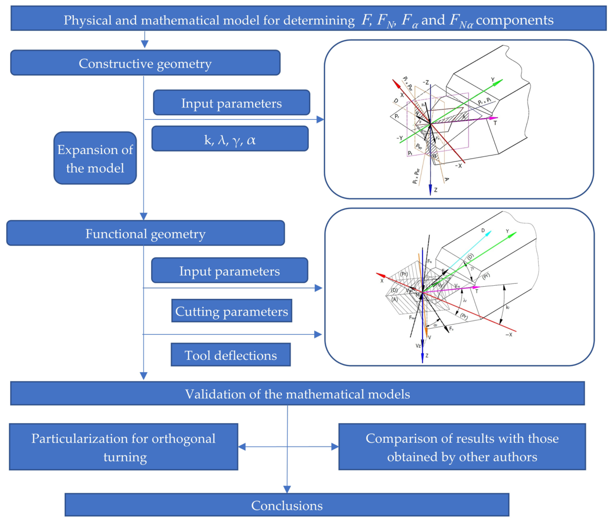
Figure 1 presents the general workflow of the proposed physical and mathematical model for determining the force components $F$, $F_N$, $F_a$, and $F_{Na}$, starting from the constructive geometry of the tool, extending toward functional geometry by incorporating cutting conditions and tool deflections. This section is devoted to the physical and mathematical development of the model, while the experimental equipment, measurement procedure, and model verification are addressed in the subsequent sections.

Symbol/Variable	Description/Definition
$\mathit{\alpha },\mathit{\gamma },\mathit{\lambda },\mathit{k}$	Constructive tool angles (clearance, rake, inclination, side cutting-edge)
${\mathit{\alpha }}_{\mathit{f}},{\mathit{\gamma }}_{\mathit{f}},{\mathit{\lambda }}_{\mathit{f}},{\mathit{k}}_{\mathit{f}}$	Dynamic functional tool angles
$\mathit{\eta }$	Chip flow direction angle
${\mathit{\theta }}_{\mathit{v}\mathit{x}},{\mathit{\theta }}_{\mathit{v}\mathit{z}}$	Cutting velocity vector orientation angles
${\mathit{\theta }}_{\mathit{y}},{\mathit{\theta }}_{\mathit{z}}$	Tool holder structural elastic deflection angles
$\mathit{F},{\mathit{F}}_{\mathit{N}}$	Friction and normal force components acting on the rake face
${\mathit{F}}_{\mathit{\alpha }},{\mathit{F}}_{\mathit{N}\mathit{\alpha }}$	Friction and normal force components acting on the flank face
${\mathit{F}}_{\mathit{x}},{\mathit{F}}_{\mathit{y}},{\mathit{F}}_{\mathit{z}}$	Global cutting force components measured by dynamometer (feed, passive, primary)

2.1. Model Principle

Studies conducted on the physical structure of cutting forces, as presented to date, have highlighted that the cutting zone is subjected to elastic deformation forces in an area preceding the separation conditions of the future chip, plastic deformation or instantaneous fracture forces—depending on whether the fracture is ductile or brittle—and internal and external friction forces [8,26,37,38].

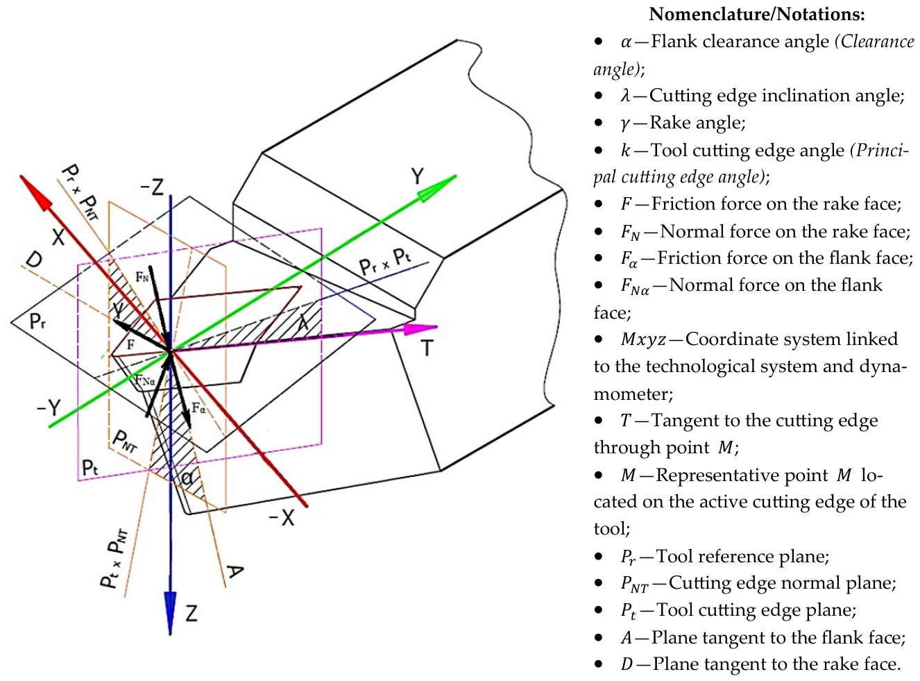
Figure 2 presents the direction and sense of the local physical components ($\overrightarrow{\mathrm{F}},\overrightarrow{{\mathrm{F}}_{\mathrm{N}}},\overrightarrow{{\mathrm{F}}_{\mathsf{\alpha }}},\overrightarrow{{\mathrm{F}}_{\mathrm{N}\mathsf{\alpha }}})$ acting at point $M$ on the cutting edge during oblique turning.

To determine the physical components of the cutting force (friction and plastic deformation), a model for oblique cutting is proposed in two variants: with a straight cutting edge and with a generalized cutting edge. These are positioned relative to a right-handed triorthogonal coordinate system, Mxyz, linked to the tool, with its origin at the considered point on the cutting edge, M, and the Mz axis oriented along the direction of the cutting velocity vector. To determine the friction and normal forces, second-rank tensors (also known as rotation matrices) were utilized via Euler angles, based on the following assumptions:

-

The tool is referenced to the coordinate system of the Kistler dynamometer, which coincides with that of the technological system;

-

The local forces are referenced to a representative point located on the active cutting edge of the tool;

-

The tool is considered a rigid body, and the actions of local tangential and normal contact force components are assumed on the active rake and flank faces;

-

The directions of the force vector components $\overrightarrow{\mathrm{F}},\overrightarrow{{\mathrm{F}}_{\mathrm{N}}},\overrightarrow{{\mathrm{F}}_{\mathsf{\alpha }}},\overrightarrow{{\mathrm{F}}_{\mathrm{N}\mathsf{\alpha }}}$ are determined by the displacement direction of the tool and the motions of the workpiece ($\overrightarrow{\mathrm{F}}$—a vector sharing the same direction as the chip rake velocity vector, and $\overrightarrow{{\mathrm{F}}_{\mathsf{\alpha }}}$—a vector sharing the same direction as the primary velocity vector, tangent to the machined surface);

-

The direction of the cutting force components is established by considering the tool as stationary, with the chip and workpiece material in motion relative to it;

-

The forces are analyzed in the cutting edge secant plane, considered at point $M$ on the tool’s cutting edge.

2.2. Physico-Mathematical Model for Cutting Tools—Constructive Geometry

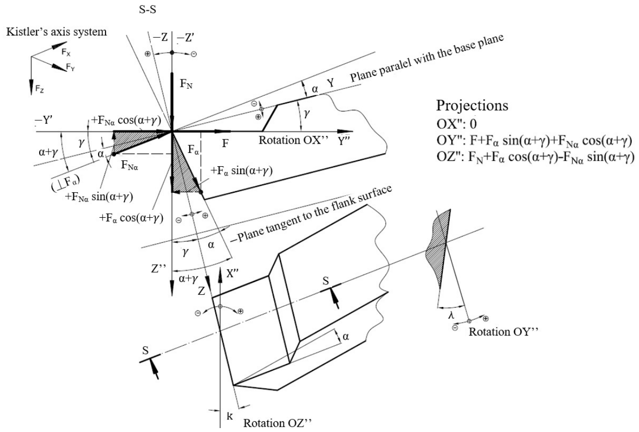
To describe the physical model and visualize the positions and directions of the cutting force physical components ($\overrightarrow{\mathrm{F}},\overrightarrow{{\mathrm{F}}_{\mathrm{N}}},\overrightarrow{{\mathrm{F}}_{\mathsf{\alpha }}},\overrightarrow{{\mathrm{F}}_{\mathrm{N}\mathsf{\alpha }}}$), a cross-section in the cutting edge secant plane was considered, as shown in Figure 3. This figure illustrates the projections of the cutting force components within the tool-bound $Mxyz$ coordinate system, which is identical to the reference system of the dynamometer. To this end, three consecutive rotations were applied to the $Mxyz$ system by angles $k$, $\lambda$, and $\gamma$ around the $Mz$, $My$, and $Mx$ axes, respectively.

The mathematical model for the physical components $F$, $F_N$, $F_{\alpha }$, and $F_{N\alpha }$, corresponding to the assumptions stated above, can be expressed in the form of Equations (1)–(4). The result of these transformations will be the product matrix (5):

$${\mathrm{R}}_{\mathrm{X}}\left(\mathsf{\gamma }\right)=\left[\begin{array}{ccc}1& 0& 0\\ 0& \cos (-\mathsf{\gamma })& \sin (-\mathsf{\gamma })\\ 0& -\sin (-\mathsf{\gamma })& \cos (-\mathsf{\gamma })\end{array}\right]$$

(1)

$${\mathrm{R}}_{\mathrm{Y}}(\mathsf{\lambda })=\left[\begin{array}{ccc}\cos (-\mathsf{\lambda })& 0& -\sin (-\mathsf{\lambda })\\ 0& 1& 0\\ \sin (-\mathsf{\lambda })& 0& \cos (-\mathsf{\lambda })\end{array}\right];$$

(2)

$${\mathrm{R}}_{\mathrm{Z}}\left(\mathrm{k}\right) =\left[\begin{array}{ccc}\cos \left(\mathrm{k}\right)& \sin \left(\mathrm{k}\right)& 0\\ -\sin \left(\mathrm{k}\right)& \cos \left(\mathrm{k}\right)& 0\\ 0& 0& 1\end{array}\right];$$

(3)

$${\mathrm{M}}_{\mathrm{tot}}=\left[\begin{array}{ccc}\cos (-\mathrm{k})& \sin (-\mathrm{k})& 0\\ -\sin (-\mathrm{k})& \cos (-\mathrm{k})& 0\\ 0& 0& 1\end{array}\right]\left[\begin{array}{ccc}\cos \left(\mathsf{\lambda }\right)& 0& \sin \left(\mathsf{\lambda }\right)\\ 0& 1& 0\\ -\sin \left(\mathsf{\lambda }\right)& 0& \cos \left(\mathsf{\lambda }\right)\end{array}\right]\left[\begin{array}{ccc}1& 0& 0\\ 0& \cos \left(\mathsf{\gamma }\right)& \sin \left(\mathsf{\gamma }\right)\\ 0& -\sin \left(\mathsf{\gamma }\right)& \cos \left(\mathsf{\gamma }\right)\end{array}\right];$$

(4)

Following a series of calculations, Equation (4) becomes:

$${\mathrm{M}}_{\mathrm{tot}}=\left[\begin{array}{ccc}\mathrm{c}\mathrm{o}\mathrm{s}\left(\mathsf{\lambda }\right)\mathrm{c}\mathrm{o}\mathrm{s}\left(\mathrm{k}\right)& \cos \left(\mathsf{\gamma }\right)\sin \left(\mathrm{k}\right)+\mathrm{s}\mathrm{i}\mathrm{n}\left(\mathsf{\gamma }\right)\mathrm{c}\mathrm{o}\mathrm{s}\left(\mathrm{k}\right)\mathrm{s}\mathrm{i}\mathrm{n}\left(\mathsf{\lambda }\right)& \cos \left(\mathsf{\gamma }\right)\mathrm{c}\mathrm{o}\mathrm{s}\left(\mathrm{k}\right)\sin \left(\mathsf{\lambda }\right)-\sin \left(\mathsf{\gamma }\right)\sin \left(\mathrm{k}\right)\\ -\left(\cos \left(\mathsf{\lambda }\right)\sin \left(\mathrm{k}\right)\right)& \cos \left(\mathsf{\gamma }\right)\cos \left(\mathrm{k}\right)-\mathrm{s}\mathrm{i}\mathrm{n}\left(\mathsf{\gamma }\right)\mathrm{s}\mathrm{i}\mathrm{n}\left(\mathsf{\lambda }\right)\mathrm{s}\mathrm{i}\mathrm{n}\left(\mathrm{k}\right)& -\left(\mathrm{s}\mathrm{i}\mathrm{n}\left(\mathsf{\gamma }\right)\mathrm{c}\mathrm{o}\mathrm{s}\left(\mathrm{k}\right)\right)-\mathrm{c}\mathrm{o}\mathrm{s}\left(\mathsf{\gamma }\right)\mathrm{s}\mathrm{i}\mathrm{n}\left(\mathsf{\lambda }\right)\mathrm{s}\mathrm{i}\mathrm{n}\left(\mathrm{k}\right)\\ -\mathrm{s}\mathrm{i}\mathrm{n}\left(\mathsf{\lambda }\right)& \mathrm{s}\mathrm{i}\mathrm{n}\left(\mathsf{\gamma }\right)\mathrm{c}\mathrm{o}\mathrm{s}\left(\mathsf{\lambda }\right)& \mathrm{c}\mathrm{o}\mathrm{s}\left(\mathsf{\gamma }\right)\mathrm{c}\mathrm{o}\mathrm{s}\left(\mathsf{\lambda }\right)\end{array}\right]$$

(5)

Rotating the coordinate system in the cutting edge secant plane by the angle $(\alpha +\gamma ),$ allows for the definition of the projections of the flank face components, $F_{\alpha }$ and $F_{N\alpha }$, onto the axes of the resulting system, as expressed in Equation (6).

$${\mathrm{R}}_{\mathrm{X}}(\mathsf{\alpha }+\mathsf{\gamma })=\left[\begin{array}{ccc}1& 0& 0\\ 0& \cos (\mathsf{\alpha }+\mathsf{\gamma })& \sin (\mathsf{\alpha }+\mathsf{\gamma })\\ 0& -\sin (\mathsf{\alpha }+\mathsf{\gamma })& \cos (\mathsf{\alpha }+\mathsf{\gamma })\end{array}\right];$$

(6)

Under these conditions, the column matrices associated with the physical components of the cutting force in the secant plane can be expressed by Equation (7). The relationship between the cutting force projections $F_x,F_y$, and $F_z$ in the $Mxyz$ coordinate system and the physical components $F,F_N,F_{\alpha }$, and $F_{N\alpha }$ in the $Mx″y″z″$ system is given by Equation (8).

$$\left[\begin{array}{c}0\\ \mathrm{F}\\ {\mathrm{F}}_{\mathrm{N}}\end{array}\right]; \mathrm{a}\mathrm{n}\mathrm{d}\left[\begin{array}{c}0\\ {\mathrm{F}}_{\mathrm{N}\mathsf{\alpha }}\\ {\mathrm{F}}_{\mathsf{\alpha }}\end{array}\right]$$

(7)

$$\left[\begin{array}{c}{\mathrm{F}}_{\mathrm{X}}\\ {\mathrm{F}}_{\mathrm{Y}}\\ {\mathrm{F}}_{\mathrm{Z}}\end{array}\right]={\mathrm{M}}_{\mathrm{t}\mathrm{o}\mathrm{t}}·\left[\begin{array}{c}0\\ \mathrm{F}\\ {\mathrm{F}}_{\mathrm{N}}\end{array}\right]+{\mathrm{R}}_{\mathrm{X}}(\mathsf{\alpha }+\mathsf{\gamma })·\left[\begin{array}{c}0\\ {\mathrm{F}}_{\mathrm{N}\mathsf{\alpha }}\\ {\mathrm{F}}_{\mathsf{\alpha }}\end{array}\right]$$

(8)

Substituting Equations (5) and (7) into Equation (8) yields equations of the form (9) and (10), respectively. In these equations, if $a_i$ ($i=1,2,3$) denote the direction parameters of the rake face friction force, $F$; $b_j$ ($j=1,2,3$) denote the direction parameters of the rake face plastic deformation force, $F_N$; $c_k$ ($k=1,2,3$) denote the direction parameters of the flank face friction force, $F_{\alpha }$; and $d_l$ ($l=1,2,3$) denote the direction parameters of the flank face normal force, $F_{N\alpha }$, then Equations (11)–(22) can be written.

$${\mathrm{M}}_{\mathrm{t}\mathrm{o}\mathrm{t}}·\left[\begin{array}{c}0\\ \mathrm{F}\\ {\mathrm{F}}_{\mathrm{N}}\end{array}\right]=\left\{\begin{array}{c}\mathrm{F}·\left(\cos \left(\mathsf{\gamma }\right)\sin \left(\mathrm{k}\right)+\sin \left(\mathsf{\gamma }\right)\sin \left(\mathsf{\lambda }\right)\cos \left(\mathrm{k}\right)\right)-{\mathrm{F}}_{\mathrm{N}}·\left(\mathrm{s}\mathrm{i}\mathrm{n}\right(\mathsf{\gamma }\left)\mathrm{s}\mathrm{i}\mathrm{n}\right(\mathrm{k})+\mathrm{c}\mathrm{o}\mathrm{s}(\mathsf{\gamma }\left)\sin \left(\mathsf{\lambda }\right)\mathrm{c}\mathrm{o}\mathrm{s}\right(\mathrm{k}\left)\right)\\ \mathrm{F}·\left(\cos \left(\mathsf{\gamma }\right)\cos \left(\mathrm{k}\right)-\sin \left(\mathsf{\gamma }\right)\sin \left(\mathsf{\lambda }\right)\sin \left(\mathrm{k}\right)\right)-{\mathrm{F}}_{\mathrm{N}}·(\mathrm{s}\mathrm{i}\mathrm{n}\left(\mathsf{\gamma }\right)\mathrm{c}\mathrm{o}\mathrm{s}\left(\mathrm{k}\right)-\mathrm{c}\mathrm{o}\mathrm{s}(\mathsf{\gamma }\left)\mathrm{s}\mathrm{i}\mathrm{n}\right(\mathsf{\lambda }\left)\mathrm{s}\mathrm{i}\mathrm{n}\right(\mathrm{k}\left)\right)\\ \mathrm{F}·\left(\sin \left(\mathsf{\gamma }\right)\cos \left(\mathsf{\lambda }\right)\right)+{\mathrm{F}}_{\mathrm{N}}·\left(\mathrm{c}\mathrm{o}\mathrm{s}\right(\mathsf{\gamma }\left)\mathrm{c}\mathrm{o}\mathrm{s}\right(\mathsf{\lambda }\left)\right)\end{array}\right.$$

(9)

$${\mathrm{R}}_{\mathrm{X}}(\mathsf{\alpha }+\mathsf{\gamma })·\left[\begin{array}{c}0\\ {\mathrm{F}}_{\mathrm{N}\mathsf{\alpha }}\\ {\mathrm{F}}_{\mathsf{\alpha }}\end{array}\right]=\left\{\begin{array}{c}0\\ {\mathrm{F}}_{\mathsf{\alpha }}·\left(\mathrm{s}\mathrm{i}\mathrm{n}\right(\mathsf{\alpha }+\mathsf{\gamma })+{\mathrm{F}}_{\mathrm{N}\mathsf{\alpha }}·\mathrm{c}\mathrm{o}\mathrm{s}(\mathsf{\alpha }+\mathsf{\gamma })\\ {\mathrm{F}}_{\mathsf{\alpha }}·\left(\mathrm{c}\mathrm{o}\mathrm{s}\right(\mathsf{\alpha }+\mathsf{\gamma }\left)\right)-{\mathrm{F}}_{\mathrm{N}\mathsf{\alpha }}·\mathrm{s}\mathrm{i}\mathrm{n}(\mathsf{\alpha }+\mathsf{\gamma })\end{array}\right.$$

(10)

$$\mathrm{a}1=\left(\cos \left(\mathsf{\gamma }\right)\sin \left(\mathrm{k}\right)+\sin \left(\mathsf{\gamma }\right)\sin \left(\mathsf{\lambda }\right)\cos \left(\mathrm{k}\right)\right)$$

(11)

$$\mathrm{a}2=\left(\cos \left(\mathsf{\gamma }\right)\cos \left(\mathrm{k}\right)-\sin \left(\mathsf{\gamma }\right)\sin \left(\mathsf{\lambda }\right)\sin \left(\mathrm{k}\right)\right)$$

(12)

$$\mathrm{a}3=\left(\sin \left(\mathsf{\gamma }\right)\cos \left(\mathsf{\lambda }\right)\right)$$

(13)

$$\mathrm{b}1=\left(\cos \right(\mathsf{\gamma }\left)\cos \right(\mathrm{k})\sin \left(\mathsf{\lambda }\right)-\sin \left(\mathsf{\gamma }\right)\sin \left(\mathrm{k}\right)$$

(14)

$$\mathrm{b}2= -(\sin \left(\mathsf{\gamma }\right)\cos \left(\mathrm{k}\right)-\cos \left(\mathsf{\gamma }\right)\sin \left(\mathsf{\lambda }\right)\sin \left(\mathrm{k}\right))$$

(15)

$$\mathrm{b}3=\left(\cos \right(\mathsf{\gamma }\left)\cos \right(\mathsf{\lambda }\left)\right)$$

(16)

$$\mathrm{c}1=0$$

(17)

$$\mathrm{c}2=\sin (\mathsf{\alpha }+\mathsf{\gamma })$$

(18)

$$\mathrm{c}3=\cos (\mathsf{\alpha }+\mathsf{\gamma })$$

(19)

$$\mathrm{d}1=0$$

(20)

$$\mathrm{d}2=\cos (\mathsf{\alpha }+\mathsf{\gamma })$$

(21)

$$\mathrm{d}3= -\sin (\mathsf{\alpha }+\mathsf{\gamma })$$

(22)

Using the notations $a_i$, $b_j$, $c_k$, and $d_l$ for the direction parameters of the components $F$, $F_N$, $F_{\alpha }$, and $F_{N\alpha }$, Equations (23) can be written, which represent an underdetermined system of three equations with four unknowns. The unknowns of the system are the local components $F$, $F_N$, $F_{\alpha }$, and $F_{N\alpha }$. For a complete solution, it is necessary to introduce additional information, either in the form of a known force component or a friction coefficient on one of the active tool faces.

$$\begin{gathered} {\mathrm{F}}_{\mathrm{x}}= \left|\mathrm{F}\right|·{\mathrm{a}}_1 +|{\mathrm{F}}_{\mathrm{N}}|·{\mathrm{b}}_1 +|{\mathrm{F}}_{\mathsf{\alpha }}|·{\mathrm{c}}_1 +|{\mathrm{F}}_{\mathrm{N}\mathsf{\alpha }}|·{\mathrm{d}}_1 \\ {\mathrm{F}}_{\mathrm{y}}= \left|\mathrm{F}\right|·{\mathrm{a}}_2 +|{\mathrm{F}}_{\mathrm{N}}|·{\mathrm{b}}_2 +|{\mathrm{F}}_{\mathsf{\alpha }}|·{\mathrm{c}}_2 +|{\mathrm{F}}_{\mathrm{N}\mathsf{\alpha }}|·{\mathrm{d}}_2 \\ {\mathrm{F}}_{\mathrm{z}}=\left|\mathrm{F}\right|·{\mathrm{a}}_3 +|{\mathrm{F}}_{\mathrm{N}}|·{\mathrm{b}}_3 +|{\mathrm{F}}_{\mathsf{\alpha }}|·{\mathrm{c}}_3 +|{\mathrm{F}}_{\mathrm{N}\mathsf{\alpha }}|·{\mathrm{d}}_3 \end{gathered}$$

(23)

Resolving the underdetermination and solving the aforementioned system of equations can be achieved by using one of the two methods:

-By determining one of the force components, which can be materialized by calculating the friction force on the flank face, ${\mathrm{F}}_{\mathsf{\alpha }}$, according to one of the methods described in the cited references. In this case, the new system of equations takes the solvable form (24):

$$\begin{gathered} {\mathrm{F}}_{\mathrm{x}}-|{\mathrm{F}}_{\mathsf{\alpha }}|·{\mathrm{d}}_1 = \left|\mathrm{F}\right|·{\mathrm{a}}_1 + |{\mathrm{F}}_{\mathrm{N}}|·{\mathrm{b}}_1 + |{\mathrm{F}}_{\mathrm{N}\mathsf{\alpha }}|·{\mathrm{c}}_1 \\ {\mathrm{F}}_{\mathrm{y}}-|{\mathrm{F}}_{\mathsf{\alpha }}|·{\mathrm{d}}_2 = \left|\mathrm{F}\right|·{\mathrm{a}}_2 + |{\mathrm{F}}_{\mathrm{N}}|·{\mathrm{b}}_2 + |{\mathrm{F}}_{\mathrm{N}\mathsf{\alpha }}|·{\mathrm{c}}_2 \\ {\mathrm{F}}_{\mathrm{z}}-|{\mathrm{F}}_{\mathsf{\alpha }}|·{\mathrm{d}}_3 = \left|\mathrm{F}\right|·{\mathrm{a}}_3 + |{\mathrm{F}}_{\mathrm{N}}|·{\mathrm{b}}_3 + |{\mathrm{F}}_{\mathrm{N}\mathsf{\alpha }}|·{\mathrm{c}}_3 \end{gathered}$$

(24)

-By knowing the friction coefficient on one of the active tool faces; for instance, if the friction coefficient on the flank face, ${\mu }_{\alpha }$, is known, the system of Equation (24) takes the form (25), whereas if the friction coefficient on the rake face, $\mu$, is known [15,27], it takes the form (26):

$$\begin{gathered} {\mathrm{F}}_{\mathrm{x}} = \left|\mathrm{F}\right|·\mathrm{a}1 + |{\mathrm{F}}_{\mathrm{N}}|·\mathrm{b}1 + \mathrm{C}1·|{\mathrm{F}}_{\mathsf{\alpha }}| \\ {\mathrm{F}}_{\mathrm{y}} = \left|\mathrm{F}\right|·\mathrm{a}2 + |{\mathrm{F}}_{\mathrm{N}}|·\mathrm{b}2 + \mathrm{C}2·|{\mathrm{F}}_{\mathsf{\alpha }}| \\ {\mathrm{F}}_{\mathrm{z}} = \left|\mathrm{F}\right|·\mathrm{a}3 + |{\mathrm{F}}_{\mathrm{N}}|·\mathrm{b}3 + \mathrm{C}3·|{\mathrm{F}}_{\mathsf{\alpha }}| \end{gathered}$$

(25)

$$\begin{gathered} {\mathrm{F}}_{\mathrm{x}}=\left|\mathrm{F}\right|·\mathrm{A}1+|{\mathrm{F}}_{\mathrm{N}\mathsf{\alpha }}|·\mathrm{c}1+|{\mathrm{F}}_{\mathsf{\alpha }}|·\mathrm{d}1 \\ {\mathrm{F}}_{\mathrm{y}}=\left|\mathrm{F}\right|·\mathrm{A}2+|{\mathrm{F}}_{\mathrm{N}\mathsf{\alpha }}|·\mathrm{c}2+|{\mathrm{F}}_{\mathsf{\alpha }}|·\mathrm{d}2 \\ {\mathrm{F}}_{\mathrm{z} }=\left|\mathrm{F}\right|·\mathrm{A}3+|{\mathrm{F}}_{\mathrm{N}\mathsf{\alpha }}|·\mathrm{c}3+|{\mathrm{F}}_{\mathsf{\alpha }}|·\mathrm{d}3 \end{gathered}$$

(26)

where the coefficients $C_i$ ($i=1,2,3$) and $A_i$ ($i=1,2,3$) are determined via Equations (27) and (28), provided that one of the friction coefficients, ${\mu }_{\alpha }$ or $\mu$, is known:

$${\mathrm{C}}_{\mathrm{i}} ={\mathrm{d}}_{\mathrm{i}} +{ \mathrm{c}}_{\mathrm{i}}·{\mathsf{\mu }}_{\mathsf{\alpha }};$$

(27)

$${ \mathrm{A}}_{\mathrm{i}}={\mathrm{a}}_{\mathrm{i}}+{ \mathrm{b}}_{\mathrm{i}}·{\mathsf{\mu }}_{\mathsf{\gamma }}$$

(28)

In the form proposed in this work, the model utilizes two categories of experimental information: the global cutting force components ($F_x,F_y,F_z$) measured with the dynamometer, and the experimentally determined friction coefficient for one of the active tool faces. Based on these data and the geometric relationships of the model, the remaining local force components are subsequently determined.

2.3. Physico-Mathematical Model for Cutting Tools—Functional Geometry

The model presented in the previous subchapter can also be formulated as a function of the tool’s functional angles. Essentially, in contrast to constructive angles—which define the cutting tool from a purely geometric perspective, independent of the machining process—functional angles define the cutting tool dynamically, in action during the actual machining process.

As is well known, incorporating functional angles into the model introduces additional input parameters alongside the constructive angles, such as cutting depth, feed rate, spindle speed, tool nose radius, and workpiece diameter. A dynamic evaluation of the tool’s state reveals that modifications occur regarding the chip flow direction ($\eta$), the functional rake angle (${\gamma }_f$), and the remaining angles, all of which are directly influenced by the cutting parameters.

The dynamic functional angles ($\eta ,{\gamma }_f$) are calculated directly from cutting parameters (feed rate $f$, workpiece diameter $D$, and side cutting-edge angle $k$) using the following analytical relations:

$$\tan \eta ={\displaystyle \frac{f\cdot \sin k}{\pi \cdot D+f\cdot \cos k}},\hspace{1em}{\tan \gamma }_f=\tan \gamma \cdot \cos \eta +\tan \lambda \cdot \sin \eta$$

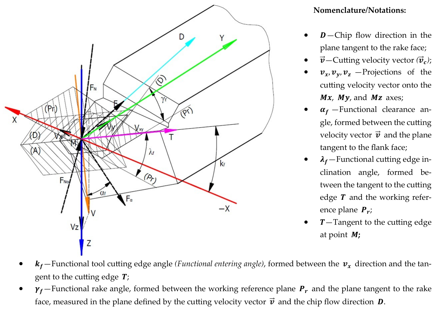
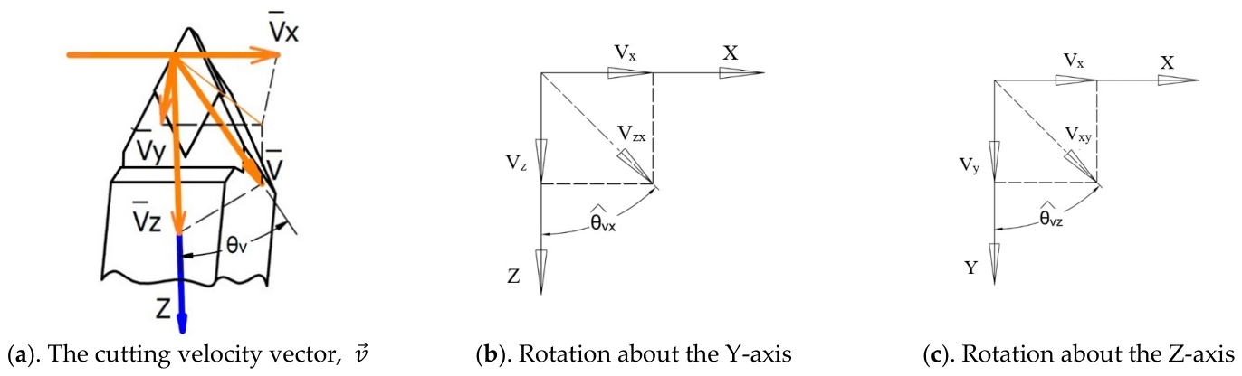
In order to extend the model to other tool geometries, the case of a tool with a straight cutting edge is presented below. This tool is referenced to the tool-bound coordinate system $Mxyz$, with its origin at an arbitrary point, $M$, located on the cutting edge. The axes are oriented as follows: the $Mz$ axis is defined along the direction of the primary cutting velocity vector ($\overrightarrow{v}$); $Mx$ is defined by the direction of the primary feed velocity vector (${\overrightarrow{v}}_f$); and the $My$ axis completes the right-handed triorthogonal coordinate system attached to the considered point $M$ (Figure 4).

The angles defining the axial directions are functional angles that depend on the most critical influencing factors related to the cutting conditions ($v$, $f$, $a_p$) and, partially, on the tool geometry (tool nose radius) and structural rigidity. The mathematical structure of the model remains unchanged; however, the constructive angles used in the rotation matrices are replaced by functional angles, which depend on the machining parameters and the actual cutting geometry.

The model proposed in this work for studying the local friction and normal force components in oblique cutting represents an adapted and simplified form of previous approaches, rewritten in terms of Euler angles and extended through the introduction of the tool’s functional angles.

In this case, the rotations of the axes as a function of the functional angles are performed primarily around the cutting velocity vector. The coefficients of the direction parameters required to solve the system of Equation (24) can be obtained by utilizing the functional angles with values determined from various relationships available in the literature [39,40].

Furthermore, this subchapter presents an original model and method regarding the possibility of calculating the physical components $F$, $F_N$, $F_{\alpha }$, and $F_{N\alpha }$ as a function of the functional geometry determined by the cutting conditions.

The expansion of the model presented in subchapter 2.1—which was formulated in terms of the tool’s constructive geometry—is achieved, as previously noted, by rotating the coordinate system in the secant plane to a position where the $Mz″$ axis aligns with the vector line of the cutting velocity, as shown in Figure 5.

$$\cos \left(\widehat{v,x}\right)={\displaystyle \frac{v_x}{\sqrt{v_x^2+v_y^2+v_z^2}}};\cos \left(\widehat{v,y}\right)={\displaystyle \frac{v_y}{\sqrt{v_x^2+v_y^2+v_z^2}}};\cos \left(\widehat{v,z}\right)={\displaystyle \frac{v_z}{\sqrt{v_x^2+v_y^2+v_z^2}}}$$

(29)

$${\mathrm{v}}_{\mathrm{x}}={\displaystyle \frac{{\mathrm{s}}_{\mathrm{l}}·\mathrm{n}}{1000}};{\mathrm{v}}_{\mathrm{y}}={\displaystyle \frac{{\mathrm{s}}_{\mathrm{t}}·\mathrm{n}}{1000}};{\mathrm{v}}_{\mathrm{z}}={\displaystyle \frac{\mathsf{\pi }·\mathrm{D}·\mathrm{n}}{1000}}$$

(30)

From Figure 5, it can be observed that in order to align the $Mz″$ axis with the vector line of the cutting velocity, two successive rotations of the coordinate system can be performed. First, the coordinate system is rotated until the $My″$ axis aligns with the projection of the cutting velocity vector, $v_{xy}$, in the $Mx″My″$ plane, followed by a rotation around the $My″$ axis. The transformation is achieved through two successive rotations: initially, a rotation within the $Mx″My″$ plane to align the projection of the cutting velocity vector, followed by a second rotation in a perpendicular plane to achieve full alignment of the $Mz″$ axis with the direction of the cutting velocity vector.

$${\mathrm{R}}_{\mathrm{Z}}=\left[\begin{array}{ccc}\cos ({\mathsf{\theta }}_{\mathrm{v}\mathrm{x}})& -\sin ({\mathsf{\theta }}_{\mathrm{v}\mathrm{x}})& 0\\ \sin ({\mathsf{\theta }}_{\mathrm{v}\mathrm{x}})& \cos ({\mathsf{\theta }}_{\mathrm{v}\mathrm{x}})& 0\\ 0& 0& 1\end{array}\right];{\mathrm{R}}_Y(V_z)=\left[\begin{array}{ccc}\cos ({\mathsf{\theta }}_{\mathrm{v}\mathrm{z}})& 0& \sin ({\mathsf{\theta }}_{\mathrm{v}\mathrm{z}})\\ 0& 1& 0\\ -\sin ({\mathsf{\theta }}_{\mathrm{v}\mathrm{z}})& 0& \cos ({\mathsf{\theta }}_{\mathrm{v}\mathrm{z}})\end{array}\right]$$

(31)

where ${\theta }_{vx}$ and ${\theta }_{vz}$ are the angles determined from the orientation of the cutting velocity vector in the local coordinate system, expressed through its direction cosines given by Equation (32).

$${\mathsf{\theta }}_{\mathrm{v}\mathrm{x}}=\mathrm{a}\mathrm{r}\mathrm{c}\mathrm{t}\mathrm{a}\mathrm{n}\left({\displaystyle \frac{{\mathrm{v}}_{\mathrm{x}}}{\sqrt{{\mathrm{v}}_{\mathrm{x}}^2+{\mathrm{v}}_{\mathrm{y}}^2+{\mathrm{v}}_{\mathrm{z}}^2}}}\right); {\mathsf{\theta }}_{\mathrm{v}\mathrm{z}}=\mathrm{a}\mathrm{r}\mathrm{c}\mathrm{c}\mathrm{o}\mathrm{s}\left({\displaystyle \frac{{\mathrm{v}}_{\mathrm{z}}}{\sqrt{{\mathrm{v}}_{\mathrm{x}}^2+{\mathrm{v}}_{\mathrm{y}}^2+{\mathrm{v}}_{\mathrm{z}}^2}}}\right)$$

(32)

The result of the transformations will be the product matrix (33), which, when applied to the $Mx″y″z″$ coordinate system, leads to Equation (34).

$${\mathrm{M}}_V=\left[\begin{array}{ccc}\mathrm{c}\mathrm{o}\mathrm{s}\left({\mathsf{\theta }}_{\mathrm{v}\mathrm{z}}\right)\mathrm{c}\mathrm{o}\mathrm{s}\left({\mathsf{\theta }}_{\mathrm{v}\mathrm{x}}\right)& -\mathrm{s}\mathrm{i}\mathrm{n}\left({\mathsf{\theta }}_{\mathrm{v}\mathrm{x}}\right)& \sin \left({\mathsf{\theta }}_{\mathrm{v}\mathrm{z}}\right)\mathrm{c}\mathrm{o}\mathrm{s}\left({\mathsf{\theta }}_{\mathrm{v}\mathrm{x}}\right)\\ \left(\cos \left({\mathsf{\theta }}_{\mathrm{v}\mathrm{z}}\right)\sin \left({\mathsf{\theta }}_{\mathrm{v}\mathrm{x}}\right)\right)& \cos \left({\mathsf{\theta }}_{\mathrm{v}\mathrm{x}}\right)& \mathrm{s}\mathrm{i}\mathrm{n}\left({\mathsf{\theta }}_{\mathrm{v}\mathrm{z}}\right)\mathrm{s}\mathrm{i}\mathrm{n}\left({\mathsf{\theta }}_{\mathrm{v}\mathrm{x}}\right)\\ -\mathrm{s}\mathrm{i}\mathrm{n}\left({\mathsf{\theta }}_{\mathrm{v}\mathrm{z}}\right)& 0& \mathrm{c}\mathrm{o}\mathrm{s}\left({\mathsf{\theta }}_{\mathrm{v}\mathrm{z}}\right)\end{array}\right]$$

(33)

$$\left[\begin{array}{c}{\mathrm{F}}_{\mathrm{X}}\\ {\mathrm{F}}_{\mathrm{Y}}\\ {\mathrm{F}}_{\mathrm{Z}}\end{array}\right]=\left\{{\mathrm{M}}_{\mathrm{t}\mathrm{o}\mathrm{t}}·\left[\begin{array}{c}0\\ \mathrm{F}\\ {\mathrm{F}}_{\mathrm{N}}\end{array}\right]+{\mathrm{R}}_{\mathrm{X}}(\mathsf{\alpha }+\mathsf{\gamma })·\left[\begin{array}{c}0\\ {\mathrm{F}}_{\mathrm{N}\mathsf{\alpha }}\\ {\mathrm{F}}_{\mathsf{\alpha }}\end{array}\right]\right\}·{\mathrm{M}}_V$$

(34)

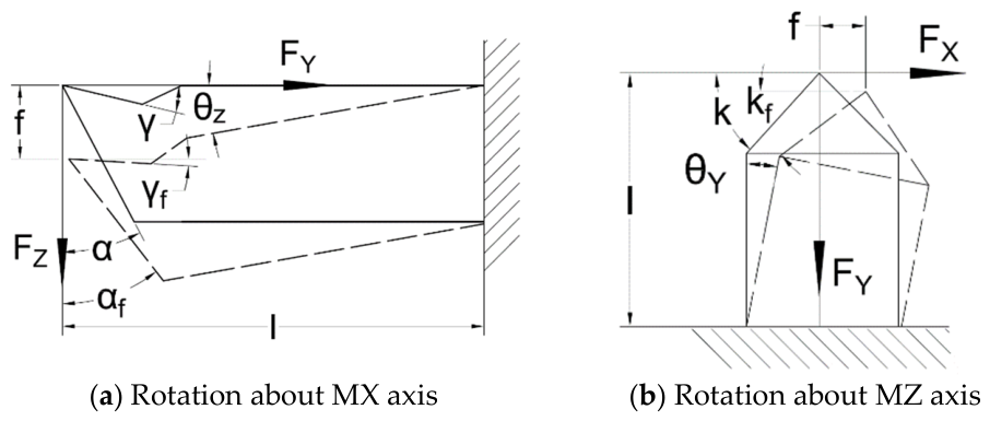
As an extension of the base model, the variation in functional geometry determined by the primary elastic deflections of the tool under the actions of the $F_z$ and $F_x$ force components can also be taken into consideration (Figure 6); thus, expression (34) takes the form (39). To incorporate the elastic deflections into the system of equations, two successive rotations were considered (Equations (35) and (38)).

$${\mathrm{R}}_{\mathrm{Z}}=\left[\begin{array}{ccc}\cos (-{\theta }_z)& \sin (-{\theta }_z)& 0\\ -\sin (-{\theta }_z)& \cos ({-\theta }_z)& 0\\ 0& 0& 1\end{array}\right]$$

(35)

As an extension of the base model, the variation in functional geometry determined by the primary elastic deflections of the tool under the actions of the $F_z$ and $F_x$ force components can also be taken into consideration (Figure 6). The structural elastic deflection angles ${\theta }_z$ and ${\theta }_y$ are calculated using Euler-Bernoulli cantilever beam mechanics applied to the unconstrained tool holder overhang ($l$) under dynamic cutting loads:

$${\theta }_z=\arctan \left({\displaystyle \frac{f_z}{l}}\right)=\arctan \left({\displaystyle \frac{F_z\cdot l^2}{3E{I}_z}}\right)\hspace{1em}$$

(36)

$${\theta }_y=\arctan \left({\displaystyle \frac{f_x}{l}}\right)=\arctan \left({\displaystyle \frac{F_x\cdot l^2}{3E{I}_z}}\right)$$

(37)

where $F_x$ and $F_z$ represent the measured dynamic cutting force components, $l$ is the tool holder overhang length, $E$ is the Young’s modulus of the tool shank material, and $I_z$ is the area moment of inertia of the tool shank cross-section. Alternatively, in high-precision setups, these deflection angles are directly mapped using dynamic static stiffness calibration coefficients ($K_{\theta }={\displaystyle \frac{\mathsf{\Delta }F}{\mathsf{\Delta }\theta }}$). To incorporate these structural elastic deflections into the system of equations, two successive rotations are performed (Equations (35) and (38)).

$${\mathrm{R}}_{\mathrm{Y}}=\left[\begin{array}{ccc}\cos ({\theta }_y)& 0& \sin ({\theta }_y)\\ 0& 1& 0\\ -\sin ({\theta }_y)& 0& \cos ({\theta }_y)\end{array}\right]$$

(38)

The result of the transformations, $M_{def}$, will be the product matrix (39).

$${\mathrm{M}}_V=\left[\begin{array}{ccc}\mathrm{c}\mathrm{o}\mathrm{s}\left({\mathsf{\theta }}_{\mathrm{v}\mathrm{z}}\right)\mathrm{c}\mathrm{o}\mathrm{s}\left({\mathsf{\theta }}_{\mathrm{v}\mathrm{x}}\right)& -\mathrm{s}\mathrm{i}\mathrm{n}\left({\mathsf{\theta }}_{\mathrm{v}\mathrm{x}}\right)& \sin \left({\mathsf{\theta }}_{\mathrm{v}\mathrm{z}}\right)\mathrm{c}\mathrm{o}\mathrm{s}\left({\mathsf{\theta }}_{\mathrm{v}\mathrm{x}}\right)\\ \left(\cos \left({\mathsf{\theta }}_{\mathrm{v}\mathrm{z}}\right)\sin \left({\mathsf{\theta }}_{\mathrm{v}\mathrm{x}}\right)\right)& \cos \left({\mathsf{\theta }}_{\mathrm{v}\mathrm{x}}\right)& \mathrm{s}\mathrm{i}\mathrm{n}\left({\mathsf{\theta }}_{\mathrm{v}\mathrm{z}}\right)\mathrm{s}\mathrm{i}\mathrm{n}\left({\mathsf{\theta }}_{\mathrm{v}\mathrm{x}}\right)\\ -\mathrm{s}\mathrm{i}\mathrm{n}\left({\mathsf{\theta }}_{\mathrm{v}\mathrm{z}}\right)& 0& \mathrm{c}\mathrm{o}\mathrm{s}\left({\mathsf{\theta }}_{\mathrm{v}\mathrm{z}}\right)\end{array}\right]$$

(39)

The final system of equations for determining the local components of the cutting force, obtained as a result of all successive rotations, takes the form of Equation (40). In this system, $A_i$ ($i=1 \mathrm{to} 3$), $B_i$ ($i=1 \mathrm{to} 3$), $C_i$ ($i=1 \mathrm{to} 3$), and $D_i$ ($i=1 \mathrm{to} 3$) represent the direction parameters along the axes of the functional coordinate system after the $M_v$ and $M_{\mathrm{def}}$ rotations, with their expressions given by Equations (41)–(52). Furthermore, $a_i$ ($i=1,2,3$), $b_j$ ($j=1,2,3$), $c_k$ ($k=1,2,3$), and $d_l$ ($l=1,2,3$) represent the direction parameters of the physical components $F$, $F_N$, $F_{\alpha }$, and $F_{N\alpha }$, given by Equations (11)–(22).

$$\left[\begin{array}{c}{\mathrm{F}}_{\mathrm{X}}\\ {\mathrm{F}}_{\mathrm{Y}}\\ {\mathrm{F}}_{\mathrm{Z}}\end{array}\right]=\left\{{\mathrm{M}}_{\mathrm{tot}}·\left[\begin{array}{c}0\\ \mathrm{F}\\ {\mathrm{F}}_{\mathrm{N}}\end{array}\right]+{\mathrm{R}}_{\mathrm{X}}(\mathsf{\alpha }+\mathsf{\gamma })·\left[\begin{array}{c}0\\ {\mathrm{F}}_{\mathrm{N}\mathsf{\alpha }}\\ {\mathrm{F}}_{\mathsf{\alpha }}\end{array}\right]\right\}·{\mathrm{M}}_{\mathrm{V}}·{\mathrm{M}}_{\mathrm{def}}$$

(40)

$${\mathrm{A}}_1={\mathrm{a}}_1 · (\mathrm{c}\mathrm{o}\mathrm{s}\left({\mathrm{V}}_{\mathrm{x}}\right)\cos \left({\mathrm{V}}_{\mathrm{z}}\right)\sin \left({\mathsf{\theta }}_{\mathrm{z}}\right)-\cos \left({\mathsf{\theta }}_{\mathrm{z}}\right)\sin \left({\mathrm{V}}_{\mathrm{x}}\right))$$

(41)

$${\mathrm{A}}_2={\mathrm{a}}_2 · \mathrm{c}\mathrm{o}\mathrm{s}\left({\mathrm{V}}_{\mathrm{z}}\right)\sin \left({\mathrm{V}}_{\mathrm{x}}\right)\sin \left({\mathsf{\theta }}_{\mathrm{z}}\right)+\cos \left({\mathsf{\theta }}_{\mathrm{z}}\right)\cos \left({\mathrm{V}}_{\mathrm{x}}\right)$$

(42)

$${\mathrm{A}}_3={\mathrm{a}}_3 · (-\left(\sin \right({\mathrm{V}}_{\mathrm{x}}\left)\sin \right({\mathsf{\theta }}_{\mathrm{z}}\left)\right)$$

(43)

$${\mathrm{B}}_1={\mathrm{b}}_1 \cos ({\mathsf{\theta }}_{\mathrm{y}}\left)\cos \right({\mathrm{V}}_{\mathrm{x}}\left)\sin \right({\mathrm{V}}_{\mathrm{z}})+\sin ({\mathsf{\theta }}_{\mathrm{y}}\left)\sin \right({\mathsf{\theta }}_{\mathrm{z}}\left)\sin \right({\mathrm{V}}_{\mathrm{x}})+\cos ({\mathrm{V}}_{\mathrm{z}}\left)\cos \right({\mathsf{\theta }}_{\mathrm{z}}\left)\cos \right({\mathrm{V}}_{\mathrm{x}})\sin ({\mathsf{\theta }}_{\mathrm{y}})$$

(44)

$${\mathrm{B}}_2={\mathrm{b}}_2 \cos ({\mathsf{\theta }}_{\mathrm{y}}\left)\sin \right({\mathrm{V}}_{\mathrm{x}}\left)\sin \right({\mathrm{V}}_{\mathrm{z}})-\sin ({\mathsf{\theta }}_{\mathrm{y}}\left)\sin \right({\mathsf{\theta }}_{\mathrm{z}}\left)\cos \right({\mathrm{V}}_{\mathrm{x}})+\cos ({\mathrm{V}}_{\mathrm{z}}\left)\cos \right({\mathsf{\theta }}_{\mathrm{z}}\left)\sin \right({\mathrm{V}}_{\mathrm{x}})\sin ({\mathsf{\theta }}_{\mathrm{y}})$$

(45)

$${\mathrm{B}}_3={\mathrm{b}}_3 \cos ({\mathrm{V}}_{\mathrm{z}})\cos ({\mathsf{\theta }}_{\mathrm{y}})-\cos ({\mathsf{\theta }}_{\mathrm{z}}\left)\sin \right({\mathrm{V}}_{\mathrm{z}})\sin ({\mathsf{\theta }}_{\mathrm{y}})$$

(46)

$${\mathrm{C}}_1 =\cos ({\mathsf{\theta }}_{\mathrm{y}})\cos ({\mathrm{V}}_{\mathrm{x}})\sin ({\mathrm{V}}_{\mathrm{z}})+\sin ({\mathsf{\theta }}_{\mathrm{y}})\sin ({\mathsf{\theta }}_{\mathrm{z}})\sin ({\mathrm{V}}_{\mathrm{x}})+\cos ({\mathrm{V}}_{\mathrm{z}})\cos ({\mathsf{\theta }}_{\mathrm{z}})\cos ({\mathrm{V}}_{\mathrm{x}})\sin ({\mathsf{\theta }}_{\mathrm{y}})$$

(47)

$${\mathrm{C}}_2={\mathrm{c}}_2 ·\cos ({\mathsf{\theta }}_{\mathrm{y}})\sin ({\mathrm{V}}_{\mathrm{x}})\sin ({\mathrm{V}}_{\mathrm{z}})-\sin ({\mathsf{\theta }}_{\mathrm{y}})\sin ({\mathsf{\theta }}_{\mathrm{z}})\cos ({\mathrm{V}}_{\mathrm{x}})+\cos ({\mathrm{V}}_{\mathrm{z}})\cos ({\mathsf{\theta }}_{\mathrm{z}})\sin ({\mathrm{V}}_{\mathrm{x}})\sin ({\mathsf{\theta }}_{\mathrm{y}})$$

(48)

$${\mathrm{C}}_3={\mathrm{c}}_3 \cos ({\mathrm{V}}_{\mathrm{z}})\cos ({\mathsf{\theta }}_{\mathrm{y}})-\cos ({\mathsf{\theta }}_{\mathrm{z}})\sin ({\mathrm{V}}_{\mathrm{z}})\sin ({\mathsf{\theta }}_{\mathrm{y}})$$

(49)

$${\mathrm{D}}_1 =\mathrm{c}\mathrm{o}\mathrm{s}\left({\mathrm{V}}_{\mathrm{x}}\right)\cos \left({\mathrm{V}}_{\mathrm{z}}\right)\sin \left({\mathsf{\theta }}_{\mathrm{z}}\right)-\cos \left({\mathsf{\theta }}_{\mathrm{z}}\right)\sin \left({\mathrm{V}}_{\mathrm{x}}\right)$$

(50)

$${\mathrm{D}}_2={\mathrm{d}}_2 ·\mathrm{c}\mathrm{o}\mathrm{s}\left({\mathrm{V}}_{\mathrm{z}}\right)\sin \left({\mathrm{V}}_{\mathrm{x}}\right)\sin \left({\mathsf{\theta }}_{\mathrm{z}}\right)+\cos \left({\mathsf{\theta }}_{\mathrm{z}}\right)\cos \left({\mathrm{V}}_{\mathrm{x}}\right)$$

(51)

$${\mathrm{D}}_3={\mathrm{d}}_3 · (-(\sin ({\mathrm{V}}_{\mathrm{x}})\sin ({\mathsf{\theta }}_{\mathrm{z}}))$$

(52)

3. Model Validation

For the purpose of validating the proposed model, its accuracy is initially verified from two perspectives: its particularization for the case where all angles are zero, and for the case of orthogonal cutting. Subsequently, experimental validation will be performed by comparing the obtained results with those available in the literature for similar conditions. These particularizations serve to verify the internal consistency of the model and its compatibility with the well-known limiting cases in cutting theory.

3.1. Physico-Mathematical Model for Cutting Tools—Constructive Geometry

To describe the physical model and visualize the positions and directions of the components, the following particularizations were considered:

I.

Particularization for the case of cutting with zero geometry in static regime

$$\mathsf{\gamma }=0°;\mathsf{\alpha }=0°;\mathrm{k}=0°;\mathsf{\lambda }=0°;{\mathrm{v}}_{\mathrm{x}}=0;{\mathrm{v}}_{\mathrm{y}}=0; {\mathrm{v}}_{\mathrm{z}}=0;$$

Thus, the values of the coefficients become:

${\mathrm{a}}_1=0;$ ${\mathrm{a}}_2=1;$ ${\mathrm{a}}_3=0;$

${\mathrm{b}}_1=0;$ ${\mathrm{b}}_2=0;$ ${\mathrm{b}}_3=1;$

${\mathrm{c}}_1=0;$ ${\mathrm{c}}_2=0;$ ${\mathrm{c}}_3=1;$

${\mathrm{d}}_1=0;$ ${\mathrm{d}}_2=1;$ ${\mathrm{d}}_3=0;$

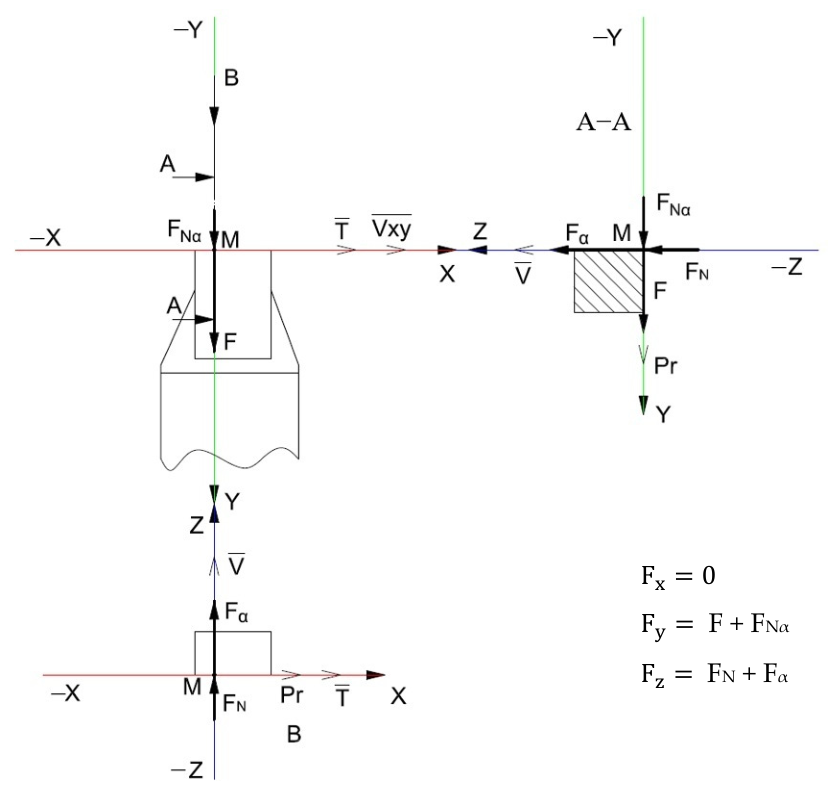
And the system of Equation (23) reduces to:

$$\begin{gathered} {\mathrm{F}}_{\mathrm{x}}=\left|\mathrm{F}\right|·0+{|\mathrm{F}}_{\mathrm{N}}|·0+{|\mathrm{F}}_{\mathsf{\alpha }}|·0+\left|{\mathrm{F}}_{\mathrm{N}\mathsf{\alpha }}\right|·0=0 \\ {\mathrm{F}}_{\mathrm{y}}=\left|\mathrm{F}\right|·1+\left|{\mathrm{F}}_{\mathrm{N}}\right|·0+{|\mathrm{F}}_{\mathsf{\alpha }}|·0+|{\mathrm{F}}_{\mathrm{N}\mathsf{\alpha }}|·1=\mathrm{F}+{\mathrm{F}}_{\mathrm{N}\mathsf{\alpha }} \\ {\mathrm{F}}_{\mathrm{z}}=\left|\mathrm{F}\right|·0+\left|{\mathrm{F}}_{\mathrm{N}}\right|·1+\left|{\mathrm{F}}_{\mathsf{\alpha }}\right|·1+\left|{\mathrm{F}}_{\mathrm{N}\mathsf{\alpha }}\right|·0={\mathrm{F}}_{\mathrm{N}}+{\mathrm{F}}_{\mathsf{\alpha }} \end{gathered}$$

(53)

Figure 7 illustrates the positions of the local cutting force components resulting from the particularization of the model for the case where all geometric angles are zero.

II.

Particularization for the Case of Orthogonal Turning

In the case of orthogonal turning, the tool’s constructive angles ($\gamma ,\alpha ,k,\lambda$), the cutting conditions ($v_x, v_y, v_z$), and the force direction parameters take the values listed below:

$\mathsf{\gamma }=0°$; $\mathsf{\alpha }=10°$; $\mathrm{k}=0°$; $\mathsf{\lambda }=0°$;

${\mathrm{v}}_{\mathrm{x}}=0°$; ${\mathrm{v}}_{\mathrm{y}}=0.18 \mathrm{m}\mathrm{m}/\mathrm{r}\mathrm{o}\mathrm{t}$; ${\mathrm{v}}_{\mathrm{z}}=157 \mathrm{m}/\mathrm{m}\mathrm{i}\mathrm{n}$;

${\mathrm{a}}_1=-0.001;$ ${\mathrm{a}}_2=1;$ ${\mathrm{a}}_3=0;$

${\mathrm{b}}_1=0.001;$ ${\mathrm{b}}_2=0;$ ${\mathrm{b}}_3=1;$

${\mathrm{c}}_1=-0.001;$ ${\mathrm{c}}_2=0.985;$ ${\mathrm{c}}_3=-0.174;$

${\mathrm{d}}_1=0.001;$ ${\mathrm{d}}_2=0.174;$ ${\mathrm{d}}_3=0.985;$

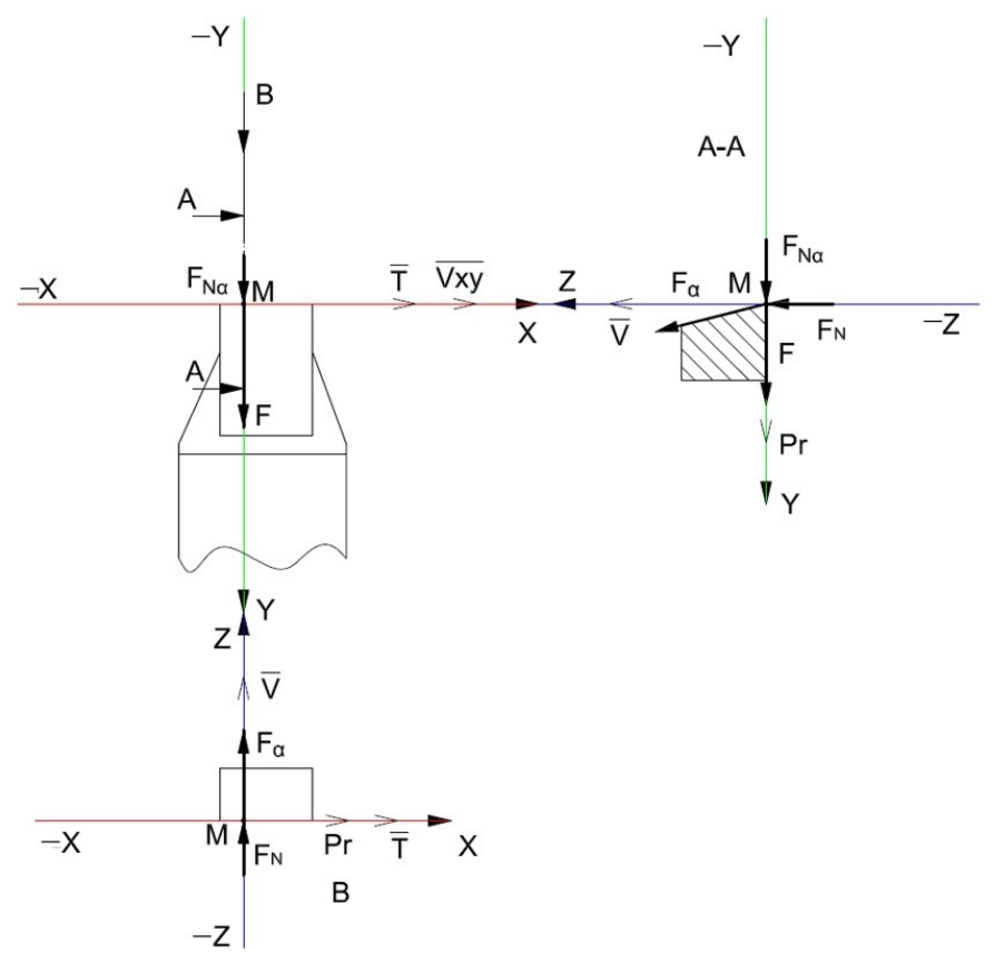
Consequently, the system of Equation (23) reduces to:

$$\begin{gathered} {\mathrm{F}}_{\mathrm{x}}=\left|\mathrm{F}\right|·-0.001+{|\mathrm{F}}_{\mathrm{N}}|·0.001+{|\mathrm{F}}_{\mathsf{\alpha }}|·-0.001+\left|{\mathrm{F}}_{\mathrm{N}\mathsf{\alpha }}\right|·0.001 \\ {\mathrm{F}}_{\mathrm{y}}=\left|\mathrm{F}\right|·1+\left|{\mathrm{F}}_{\mathrm{N}}\right|·0+{|\mathrm{F}}_{\mathsf{\alpha }}|·0.985+|{\mathrm{F}}_{\mathrm{N}\mathsf{\alpha }}|·0.174 \\ {\mathrm{F}}_{\mathrm{z}}=\left|\mathrm{F}\right|·0+\left|{\mathrm{F}}_{\mathrm{N}}\right|·1+\left|{\mathrm{F}}_{\mathsf{\alpha }}\right|·-0.174+\left|{\mathrm{F}}_{\mathrm{N}\mathsf{\alpha }}\right|·0.985 \end{gathered}$$

(54)

The graphical representation of orthogonal turning, illustrated in Figure 8, verifies the correctness and accuracy of this particularized case.

3.2. Experimental Validation

For the implementation of the model as well as for the first-stage experimental validation, it was necessary to acquire the input parameters $F_x$, $F_y$, and $F_z$. To resolve the underdetermination of the system of Equation (40), the friction coefficient on the flank face was determined using a tribometer described in [41].

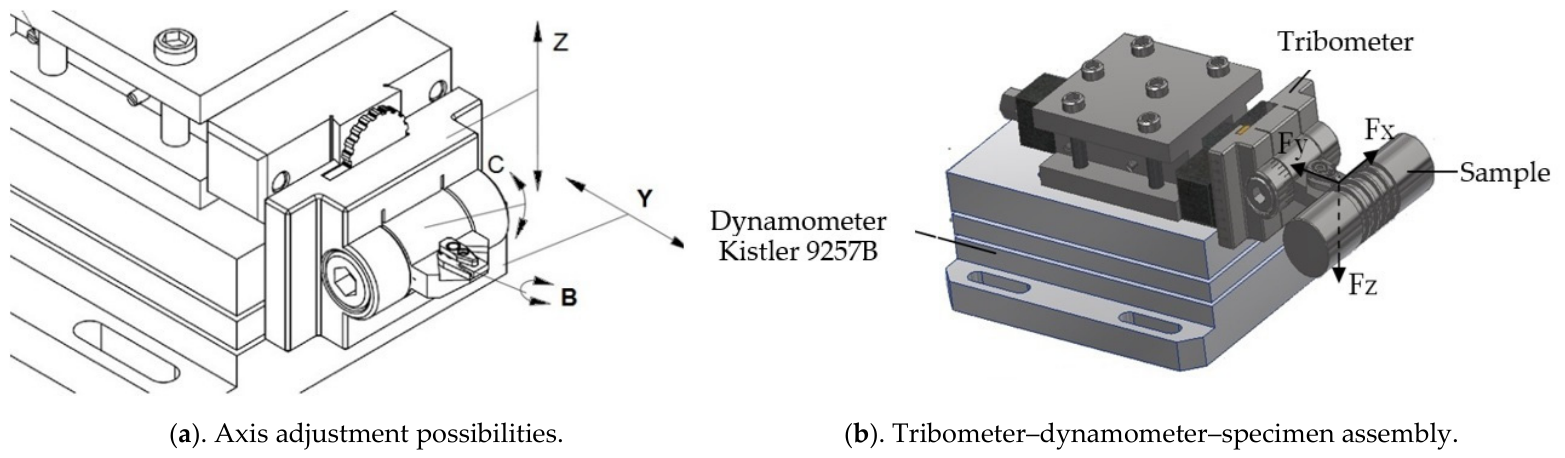
The tribometer, designed and manufactured in a flexible manner to allow adjustments for achieving different values of the entering angle, rake angle, and clearance angle, is mounted on a highly sensitive Kistler 9257B piezoelectric dynamometer, which enables the measurement of the cutting force components ($F_x,F_y$, and $F_z$).

The insert, mechanically clamped onto the tribometric device—which, in turn, is fixed to the Kistler dynamometer—is pressed against the specimen made of the investigated material until the desired pressure is achieved on the contact surface (Figure 9).

The friction coefficient was determined by calculating the ratio of the $F_z$ component values (acting as the friction force in this case) to the $F_y$ component values (the normal/pressing force). The tribometer is capable of replicating various cutting tool geometries by repositioning the insert within the fixture, thereby enabling the determination of the friction coefficient on both active tool faces (the rake and flank faces, respectively).

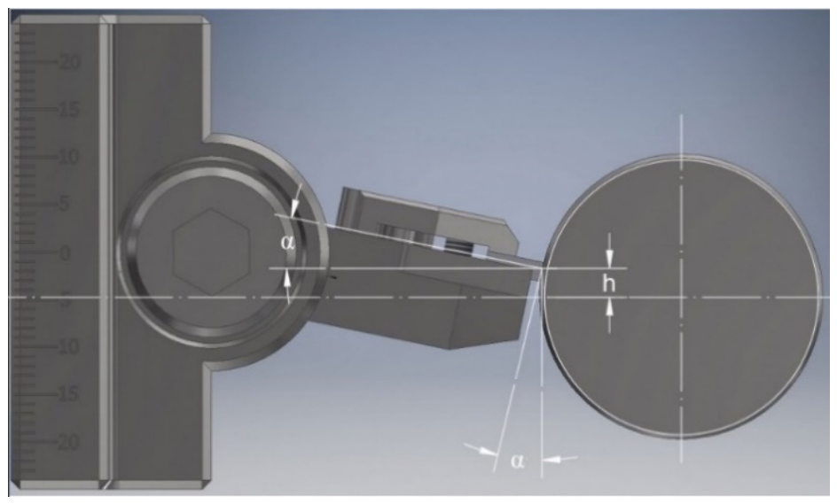
In order to simulate the clearance angle and eliminate the possibility of actual cutting, it was necessary to elevate the tribometric device, as shown in Figure 10. The height value required for the effective simulation of the clearance angle is given by Equation (51), where $R$ denotes the radius of the workpiece, $h$ represents the elevation height, and $\alpha$ is the clearance angle.

$$h=R·tg(\alpha )$$

(55)

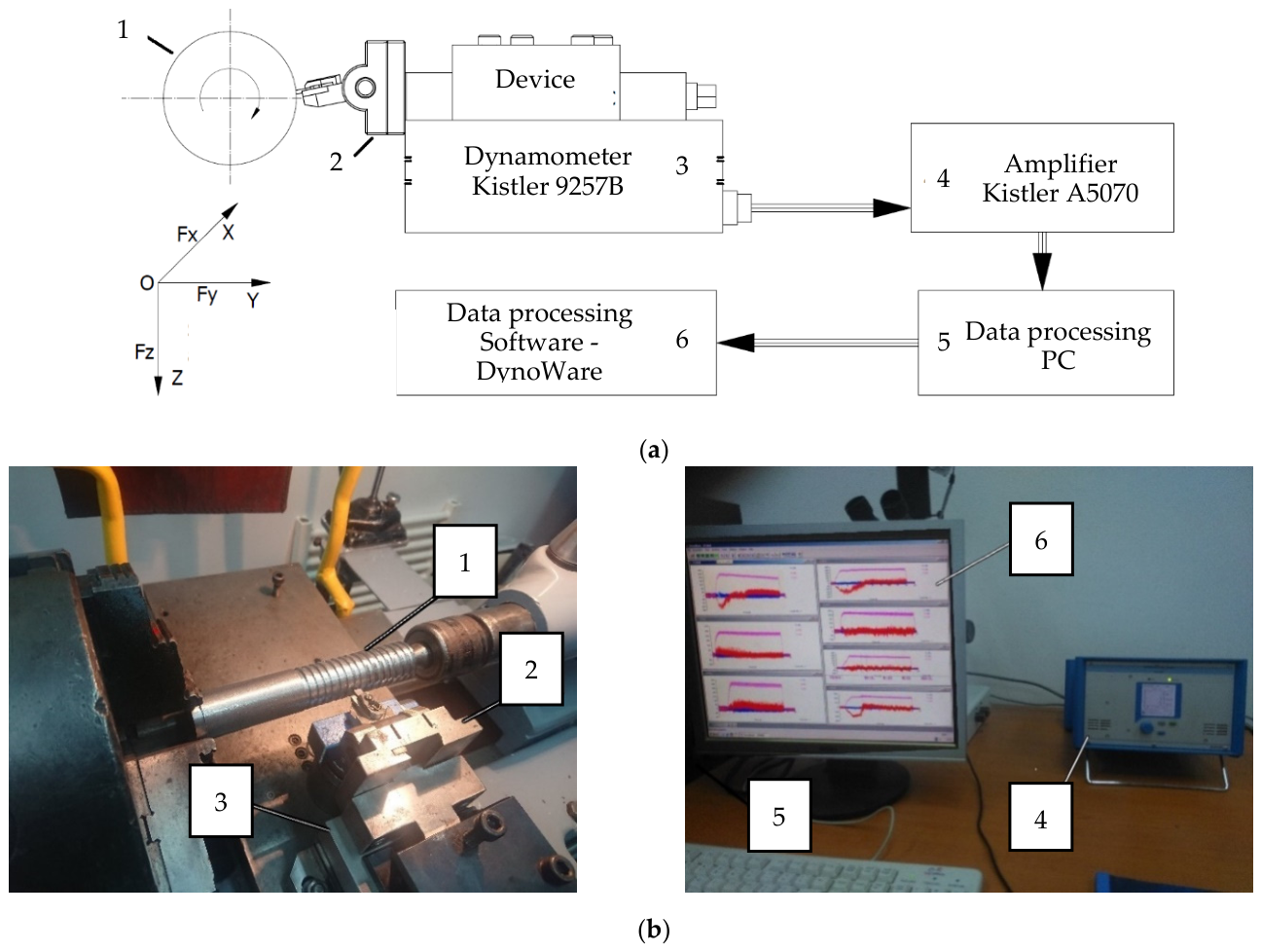
The measuring chain—consisting of the specimen (1), the tribometric device (2), the dynamometer (3), the charge amplifier (4), the PC (5), and a specialized data processing software presented in Figure 11—was utilized both for determining the friction coefficients and for studying the influence of the cutting conditions ($v,f,a_p$) and tool geometry on these coefficients. The experimental conditions are described in

Table 1. Theoretical and experimental results obtained during the turning of C45 steel, using the model based on design angles.

Nr.	Input Parameters			Experimental Results			Parameters Obtained Using the Presented Model
	Principal Cutting Edge Angle	Cutting Speed	Cutting Feed	Force Values Obtained with the Kistler Dynamometer			Values Determined Using the Proposed Model, Equation (40)					The Coefficient of Friction, µα, Determined Using the Tribometer.
	k [°]	v [m/min]	f [mm/rev]	Fx [N]	Fy [N]	Fz [N]	F [N]	FN [N]	Fα [N]	FNα [N]	μγ	${\mathsf{\mu }}_{\mathsf{\alpha }}$
1	90	98.91	0.18	167.98	216.61	289.63	140.53	269.93	37.26	190.08	0.521	0.196
2			0.28	201.77	317.74	406.70	163.37	375.91	51.88	280.45	0.435	0.185
3			0.36	207.63	370.70	463.77	163.78	428.08	57.40	327.99	0.383	0.175
4		125.6	0.18	174.09	217.08	302.11	145.10	284.96	35.35	189.04	0.509	0.187
5			0.28	203.27	328.85	405.26	164.93	375.47	51.03	291.62	0.439	0.175
6			0.36	191.35	332.62	445.80	148.61	416.63	49.17	290.93	0.357	0.169
7		157	0.18	158.30	209.06	285.81	130.67	271.18	31.17	182.30	0.482	0.171
8			0.28	183.78	288.36	382.49	146.66	362.86	38.85	252.24	0.404	0.154
9			0.36	173.40	317.85	433.58	131.33	409.37	42.34	276.73	0.321	0.153
10	70	98.91	0.18	236.68	317.21	423.72	224.76	411.51	40.08	188.16	0.546	0.213
11			0.28	279.12	445.30	541.82	263.14	514.21	60.59	289.88	0.512	0.209
12			0.36	309.25	556.40	665.83	287.58	628.97	73.63	377.61	0.457	0.195
13		125.6	0.18	244.21	304.76	413.09	232.96	409.02	32.76	173.34	0.57	0.189
14			0.28	271.38	408.53	531.19	254.59	518.64	44.69	255.34	0.491	0.175
15			0.36	276.88	454.99	604.21	255.65	590.54	46.70	291.86	0.433	0.16
16		157	0.18	218.15	268.55	373.30	207.41	375.72	23.25	150.00	0.552	0.155
17			0.28	242.04	360.00	499.82	224.95	494.31	34.29	219.84	0.455	0.156
18			0.36	208.81	414.94	556.93	186.11	545.46	36.78	280.76	0.341	0.131
19	45	98.91	0.18	222.29	359.87	397.76	312.43	409.21	25.50	82.25	0.763	0.31
20			0.28	290.66	526.47	557.49	408.51	564.09	42.03	159.19	0.724	0.264
21			0.36	311.06	608.98	632.56	437.16	633.75	51.18	211.50	0.69	0.242
22		125.6	0.18	249.96	379.21	410.27	351.34	431.04	20.47	71.31	0.815	0.287
23			0.28	305.02	520.78	553.35	428.70	564.94	39.15	139.33	0.759	0.281
24			0.36	288.53	579.24	605.32	405.49	606.08	48.02	207.87	0.669	0.231
25		157	0.18	238.16	350.01	400.55	334.74	427.79	12.23	54.13	0.782	0.226
26			0.28	282.36	464.40	526.94	396.84	554.74	19.51	106.62	0.715	0.183
27			0.36	393.85	603.13	799.31	553.48	852.66	13.50	92.48	0.649	0.146

.

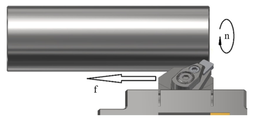
The experimental runs for validating the previously presented model were conducted on an SN 320 × 750 universal lathe. The simulation of the entering angle was carried out according to Figure 12.

The machined material was a high-quality carbon steel, C45 EN 10083-1 (equivalent to AISI 1045), frequently used in machine manufacturing. A P20 cemented carbide insert was used as the active cutting part of the tool, with the geometry provided by a PCLNR 2525 M 12 tool holder. The constructive angles of the tool consist of: $\alpha =-6^{\circ }$, $\gamma =6^{\circ }$, and $\lambda =6^{\circ }$.

To this end, a set of trials was organized based on a $3^3$ Design of Experiments (DOE) plan to determine the flank friction coefficient, ${\mu }_{\alpha }$. Each cutting condition combination was evaluated through a single continuous experimental trial ($n=1$) due to material and experimental setup constraints. To guarantee high data reliability despite single-run trials, cutting force signals were acquired continuously at high sampling frequency across the full length of the pass. Only the fully stabilized steady-state region of the force profile was extracted, and Grubbs’ statistical test ($\alpha =0.05$) was applied to automatically identify and eliminate high-frequency acquisition noise and physical signal disturbances. Using the resulting steady-state mean values for the $F_x$, $F_y$, and $F_z$ components, the remaining local physical force components were calculated via Equation (25) and are summarized in Table 1.

Quantitative error evaluation confirms high model accuracy, with relative force reconstruction errors remaining strictly below the 3.5% critical threshold. Specifically, relative errors ranged between 1.2% and 2.8% for the primary cutting force ($F_z$), and between 1.8% and 3.4% for feed and passive forces ($F_x,F_y$). Mechanistically, increasing feed rate ($f$) increases chip area, driving up normal force components ($F_N,F_{N\alpha }$), while higher cutting speeds ($v$) cause thermal softening that reduces the rake friction coefficient ${\mu }_{\gamma }$.

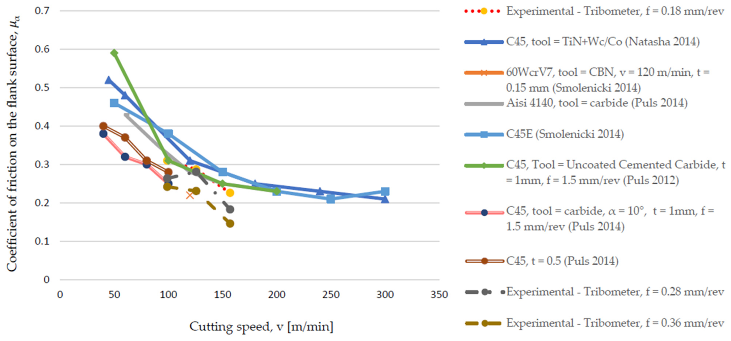
Figure 13 presents a comparison between the friction coefficients measured on the flank face using the tribometer described previously in this work, across the three feed rates and cutting speeds considered in the conducted experiments. The corresponding friction coefficient values obtained within the Taguchi experimental design can be considered a validation of the proposed model, as they are in close agreement with those reported by other authors [16,17,19,42].

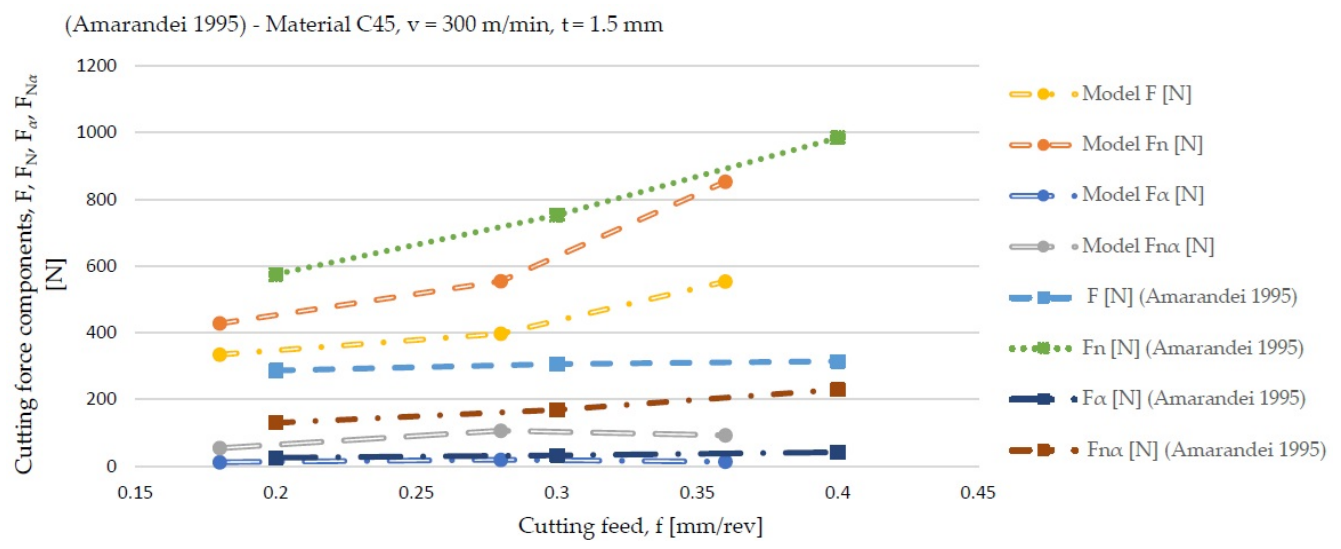
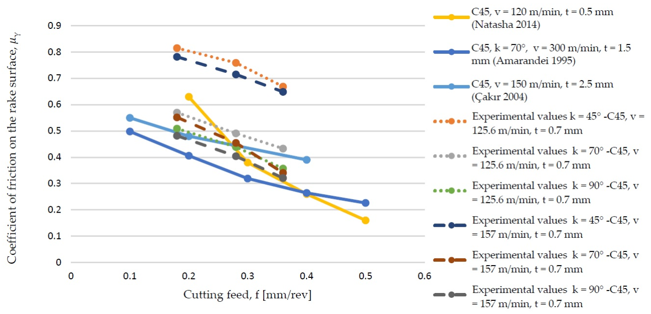
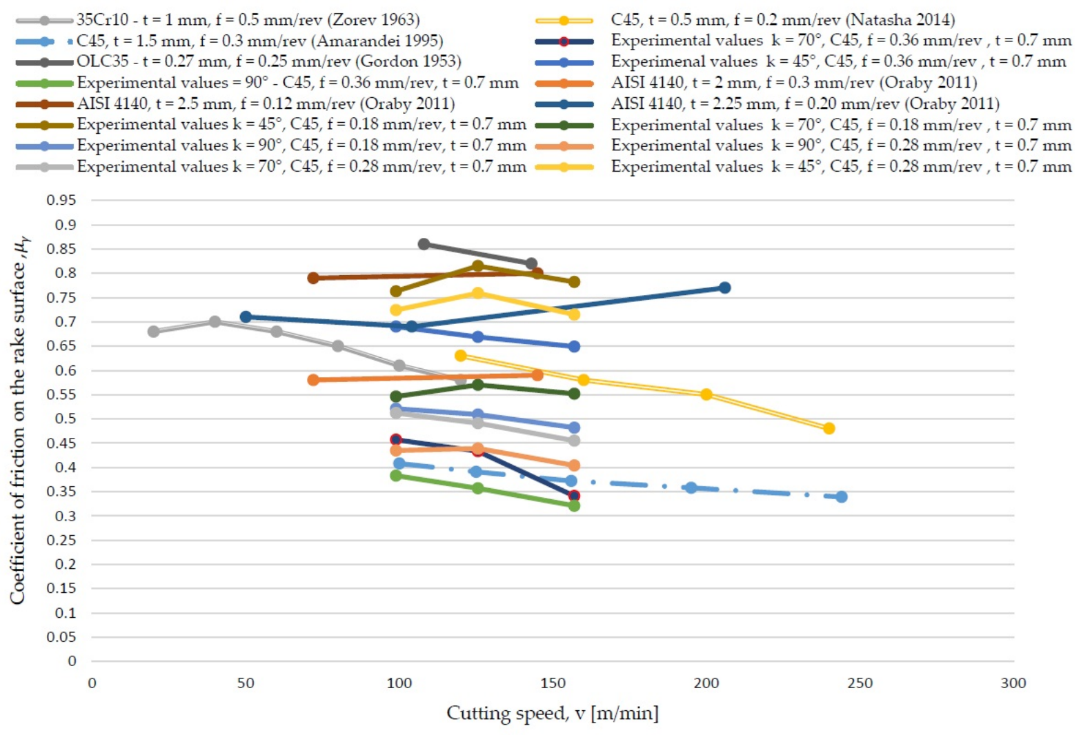
The validation of the model described by Equation (54), performed for the case of semi-orthogonal cutting with the tool geometric and working parameters listed in Table 1, is also demonstrated by the plotted dependencies for the friction coefficient and the $F,F_N,F_{\alpha },F_{N\alpha }$ components presented in Figure 14, Figure 15 and Figure 16. It is found that the values obtained for the rake face friction coefficient show a strong tendency to align with similar variations reported in the literature [42,43,44,45,46,47,48], occupying a median position.

3.3. Partial Conclusions Regarding the Experimental Validation of the Model

Based on the analysis and interpretation of the experimental results presented in this subsection, the following main conclusions have been drawn:

• Theoretical validation through particularization: Particularizing the proposed analytical–mechanistic model for the case of orthogonal cutting demonstrates a clear convergence with the classic Merchant model [5]. Furthermore, the vector force distributions illustrated in Figure 3 and Figure 4 faithfully correspond to the actual kinematics of the real cutting zone.
• Tribological behavior on the rake face: The variation in the local friction coefficient on the tool’s rake face, as well as the trend of the experimental curves plotted within the cutting speed range of $v_c\in \left[90\dots 160\right] \mathrm{m}/\min$, shows a strong correlation with the evolutionary patterns and trends identified by other authors for similar machining processes performed within the same kinematic windows (Figure 16).
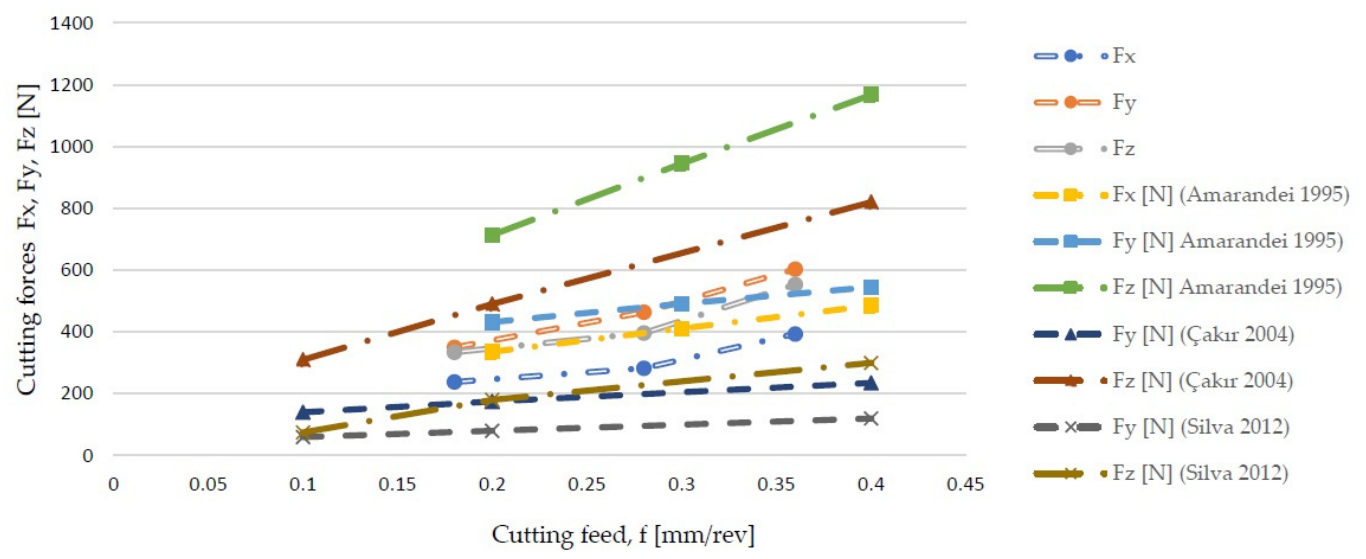
• Correlation of cutting force components: The trend of the variation curves for the orthogonal cutting force components ($F_X$, $F_Y$, and $F_Z$), plotted using the data centralized in Table 1, is highly consistent with the profiles reported in the specialized literature [47,48]. Additionally, the numerical values of the physical components and friction coefficients calculated via the proposed model for the same technological input parameters show high statistical proximity to the results reported in [42,43,46,47], falling strictly within the accepted variability limits (Figure 17).
• Statistical data validation: The application of the Grubbs statistical tests to identify and eliminate gross errors (outliers), carried out according to the methodology outlined in reference [44,49], demonstrates high stability of the experimental dataset, with the maximum calculated error not exceeding the critical threshold of $3.5\%$. Specifically, relative reconstruction errors for the primary cutting force ($F_z$) ranged between 1.2% and 2.8%, while feed and passive forces ($F_x,F_y$) exhibited errors between 1.8% and 3.4%, remaining strictly below the critical threshold of 3.5%.

Given these convergent findings, the working hypothesis is confirmed, and the utility of the proposed model is fully validated for predicting and studying plastic deformation forces, friction forces, and friction coefficients in cutting operations, guaranteeing high computational accuracy and scientific resolution for production engineering applications.

4. Conclusions

The theoretical and experimental research presented in this paper has achieved the proposed objectives, providing a clear picture of machining phenomenology and the accurate determination of local friction forces. Based on the results obtained, the following general conclusions can be drawn:

• The proposed analytical-mechanistic model for determining local friction forces and normal forces in oblique machining has been successfully validated both theoretically and experimentally. Its adaptation to the specific case of orthogonal machining confirms mathematical convergence with the classical equations of the Merchant model.
• The study of tribological behavior on the cutting tool’s rake face revealed that the shape of the experimental curves for the local velocity coefficient within the local velocity range (up to 160 m/min) adheres strictly to the physical laws governing machining processes. This strong correlation demonstrates the model’s high predictive capability.
• The force distribution vector diagrams accurately reflect the reality of the secondary plastic deformation zone. The orthogonal cutting force components ($F_x,F_y,F_z$) calculated using the proposed model show excellent statistical proximity to internationally validated reference values. Keeping gross errors below the critical threshold of 3.5% ensures the reproducibility of results and the scientific validity of the model.
• The tribometric device employed in this study allows for the isolated investigation of temperature variation and cutting process physics at the tool–workpiece interface, specifically within the flank face region. By isolating the flank face, this approach contributes to a better understanding of tool transverse wear mechanisms.

Single-Point Load Assumption and Future Work: It should be noted that the present model assumes local forces are reported at a single representative point along the active cutting edge. This simplification was intentionally chosen to balance analytical rigor with computational efficiency, providing a robust and fast mathematical framework for force transformation without heavy computational overhead. Although a single-point representation omits the continuous, non-uniform distribution of contact pressures and progressive tool wear along the contact length, it establishes the necessary foundation for turning optimization. Future developments will expand this model by discretizing the cutting edge into finite segments, allowing localized stress distributions and progressive tool wear dynamics to be modeled in detail.

Originality and Scientific Contribution: The main elements of originality and added value introduced by this work consist of the development of an extended analytical-mechanistic model using Euler rotation matrices capable of estimating local normal and friction forces under complex oblique cutting conditions, thereby overcoming the simplifying limitations of classical two-dimensional models. Furthermore, the implementation of a statistical validation algorithm based on significance tests (such as Grubbs) ensures the automatic elimination of disturbances and signal noise acquired during the cutting process.

References

1. Shi, B.; Attia, M.H. Current status and future direction in the numerical modeling and simulation of machining processes: A critical literature review. Mach. Sci. Technol. 2010, 14, 149–188. [Google Scholar] [CrossRef] [Scilit]
2. Neugebauer, R.; Bouzakis, K.D.; Denkena, B.; Klocke, F.; Sterzing, A.; Tekkaya, A.E.; Wertheim, R. Velocity effects in metal forming and machining processes. CIRP Ann. Manuf. Technol. 2011, 60, 627–650. [Google Scholar] [CrossRef] [Scilit]
3. Abouridouane, M.; Bergs, T.; Schraknepper, D.; Wirtz, G. Friction behavior in metal cutting: Modeling and simulation. Procedia CIRP 2021, 102, 405–410. [Google Scholar] [CrossRef] [Scilit]
4. Arrazola, P.J.; Özel, T.; Umbrello, D.; Davies, M.; Jawahir, I.S. Recent advances in modelling of metal machining processes. CIRP Ann. Manuf. Technol. 2013, 62, 695–718. [Google Scholar] [CrossRef] [Scilit]
5. Merchant, M.E. Mechanics of the metal cutting process. I. Orthogonal cutting and a type 2 chip. J. Appl. Phys. 1945, 16, 267–275. [Google Scholar] [CrossRef] [Scilit]
6. Armarego, E.J.A.; Brown, R.H. The Machining of Metals; Prentice-Hall: Englewood Cliffs, NJ, USA, 1977. [Google Scholar]
7. Wang, J.; Liu, C.R. The effect of tool flank wear on the heat transfer, thermal damage and cutting mechanics in finish hard turning. CIRP Ann. Manuf. Technol. 1999, 48, 53–58. [Google Scholar] [CrossRef] [Scilit]
8. Milutinović, M.; Tanović, L. Cutting forces in hard turning comprising tool flank wear and its implication for the friction between tool and workpiece. Teh. Vjesn. Tech. Gaz. 2016, 23, 1373–1379. [Google Scholar] [CrossRef] [Scilit][Green Version]
9. Lee, E.H.; Shaffer, B.W. The theory of plasticity applied to a problem of machining. J. Appl. Mech. 1951, 18, 405–413. [Google Scholar] [CrossRef] [Scilit]
10. Ackroyd, B.; Chandrasekar, S.; Compton, W.D. A model for the contact conditions at the chip-tool interface in machining. J. Tribol. 2003, 125, 649–660. [Google Scholar] [CrossRef] [Scilit]
11. Astakhov, V.P. Tribology of Metal Cutting; Elsevier: Amsterdam, The Netherlands, 2006. [Google Scholar]
12. Filice, L.; Micari, F.; Rizzuti, S.; Umbrello, D. A critical analysis on the friction modelling in orthogonal machining. Int. J. Mach. Tools Manuf. 2007, 47, 709–714. [Google Scholar] [CrossRef] [Scilit]
13. Grzesik, W.; Żak, K. Friction quantification in the oblique cutting with CBN chamfered tools. Wear 2013, 304, 36–42. [Google Scholar] [CrossRef] [Scilit]
14. Melkote, S.N.; Grzesik, W.; Outeiro, J.; Rech, J.; Schulze, V.; Attia, H.; Arrazola, P.J.; M’Saoubi, R.; Saldana, C. Advances in material and friction data for modelling of metal machining. CIRP Ann. Manuf. Technol. 2017, 66, 731–754. [Google Scholar] [CrossRef] [Scilit]
15. Grzesik, W.; Rech, J.; Żak, K. Determination of friction in metal cutting with tool wear and flank face effects. Wear 2014, 317, 8–16. [Google Scholar] [CrossRef] [Scilit]
16. Puls, H.; Klocke, F.; Lung, D. A new experimental methodology to analyse the friction behaviour at the tool-chip interface in metal cutting. Prod. Eng. Res. Dev. 2012, 6, 349–354. [Google Scholar] [CrossRef] [Scilit]
17. Puls, H.; Klocke, F.; Lung, D. Experimental investigation on friction under metal cutting conditions. Wear 2014, 310, 63–71. [Google Scholar] [CrossRef] [Scilit]
18. Voss, R.; Seeholzer, L.; Kuster, F.; Wegener, K. Cutting process tribometer experiments for evaluation of friction coefficient close to a CFRP machining operation. Procedia CIRP 2017, 66, 204–209. [Google Scholar] [CrossRef] [Scilit]
19. Smolenicki, D.; Boos, J.; Kuster, F.; Roefolds, H.; Wyen, C. In-process measurement of friction coefficient in orthogonal cutting. CIRP Ann. Manuf. Technol. 2014, 63, 97–100. [Google Scholar] [CrossRef] [Scilit]
20. Zemzemi, F.; Bensalem, W.; Rech, J.; Dogui, A.; Kapsa, P. New tribometer design designed for the characterisation of the friction properties at the tool/chip/workpiece interface in machining. Tribotest 2008, 14, 11–25. [Google Scholar] [CrossRef] [Scilit]
21. Zemzemi, F.; Rech, J.; Salem, W.B.; Dogui, A.; Kapsa, P. Identification of a friction model at tool/chip/workpiece interfaces in dry machining of AISI4142 treated steels. J. Mater. Process. Technol. 2009, 209, 3978–3990. [Google Scholar] [CrossRef] [Scilit]
22. Hedenqvist, P.; Olsson, M. Sliding wear testing of coated cutting tool materials. Tribol. Int. 1991, 24, 143–150. [Google Scholar] [CrossRef] [Scilit]
23. Naisson, P.; Rech, J.; Paris, H. Characterization of friction properties during machining of various stainless steels. Eng. Trans. 2013, 61, 239–248. [Google Scholar]
24. Rech, J.; Claudin, C.; Polly, P.; Courbon, C. New aspects of metrology of frictional behaviour in metal cutting. Mechanik 2016, 11, 1751–1753. [Google Scholar] [CrossRef] [Scilit]
25. Rech, J.; Claudin, C.; Grzesik, W.; Zalisz, Z. Characterization of the friction properties of various coatings at the tool-chip-workpiece interfaces in dry machining of AISI 4140 steel. Proc. Inst. Mech. Eng. Part J J. Eng. Tribol. 2008, 222, 617–627. [Google Scholar] [CrossRef] [Scilit]
26. Zhang, C.; Lu, J.; Zhang, F.; Butt, S.I. Identification of a new friction model at tool-chip interface in dry orthogonal cutting. Int. J. Adv. Manuf. Technol. 2017, 89, 921–932. [Google Scholar] [CrossRef] [Scilit]
27. Zhang, G.; Guo, C. Modeling of cutting force distribution on tool edge in turning process. Procedia Manuf. 2015, 1, 454–465. [Google Scholar] [CrossRef] [Scilit]
28. Grzesik, W.; Kowalczyk, D.; Żak, K. A new mechanistic friction model for the oblique cutting with tool wear effect. Tribol. Int. 2013, 66, 49–53. [Google Scholar] [CrossRef] [Scilit]
29. Childs, T.H.C. Friction modelling in metal cutting. Wear 2006, 260, 310–318. [Google Scholar] [CrossRef] [Scilit]
30. Campocasso, S.; Costes, J.P.; Fromentin, G.; Bissey-Breton, S.; Poulachon, G. A generalized geometrical model of turning operations for cutting force modelling using edge discretization. Appl. Math. Model. 2015, 39, 6612–6630. [Google Scholar] [CrossRef] [Scilit]
31. Song, G.; Sui, S.; Tang, L. Precision prediction of cutting force in oblique cutting operation. Int. J. Adv. Manuf. Technol. 2015, 81, 553–562. [Google Scholar] [CrossRef] [Scilit]
32. Dorlin, T.; Fromentin, G.; Costes, J.P.; Karaouni, H. Mechanistic cutting force model including the stress state induced by the chip flow contribution for cylindrical turning on Ti6Al4V alloy with two different nose radii. In Proceedings of the 13th International Conference on High Speed Machining, Metz, France, 4–5 October 2016. [Google Scholar]
33. Bera, T.C.; Manikandan, H.; Bansal, A.; Nema, D. A method to determine cutting force coefficients in turning using mechanistic approach. Int. J. Mater. Mech. Manuf. 2018, 6, 99–103. [Google Scholar] [CrossRef] [Scilit][Green Version]
34. Moufki, A.; Molinari, A.; Dudzinski, D. Modelling of orthogonal cutting with a temperature dependent friction law. J. Mech. Phys. Solids 1998, 46, 2103–2138. [Google Scholar] [CrossRef] [Scilit]
35. Ozlu, E.; Budak, E. Experimental analysis and modeling of orthogonal cutting using material and friction models. In Proceedings of the 4th International Conference and Exhibition on Design and Production of Machines and DIES/MOLDS, Cesme, Turkey, 21–23 June 2007. [Google Scholar]
36. Huerta, L.; Lozano-Guzman, A.; Orozco-Mendoza, H.; Jauregui-Correa, J.C. Method for friction force estimation on the flank of cutting tools. Shock. Vib. 2017, 2017, 5834863. [Google Scholar] [CrossRef] [Scilit]
37. Molinari, A.; Dudzinski, D. Stationary shear band in high-speed machining. Comptes Rendus Acad. Sci. 1991, 315, 399–405. [Google Scholar]
38. Lin, X.; Yang, W.; Xu, D.; Li, W.; Ma, S. Internal friction and compressive deformation in the primary zone during the high-speed cutting of SiCp/Al composites. arXiv 2021, arXiv:2103.17047. [Google Scholar]
39. Belous, V. Sinteza Sculelor Așchietoare [Synthesis of Cutting Tools]; Junimea: Iași, Romania, 1980. [Google Scholar]
40. Kiyak, M.; Altan, M.; Altan, E. Prediction of chip flow angle in orthogonal turning of mild steel by neural network approach. Int. J. Adv. Manuf. Technol. 2007, 33, 251–259. [Google Scholar] [CrossRef] [Scilit]
41. Tamasag, I.; Beșliu, I.; Amarandei, D. Design of a device for testing and analysing the friction coefficient during metal cutting. Ann. Oradea Univ. Fascicle Manag. Technol. Eng. 2019, 28, 85–90. [Google Scholar]
42. Natasha, A.R.; Othman, H.; Jaharah, A.G.; Che Haron, C.H.; Syarif, J. Chip formation and coefficient of friction in turning S45C medium carbon steel. Int. J. Mech. Mechatron. Eng. 2014, 14, 89–92. [Google Scholar]
43. Amarandei, D. Experimental method applied for modelling edge tool cutting with aim of evaluation the plastic deformation forces and friction forces at high speed machining. In Proceedings of the 4th Yugoslav Conference of Tribology, Belgrade, Serbia, 27–29 September 1995. [Google Scholar]
44. Çakır, O.; Kıyak, M.; Altan, E. Comparison of gases applications to wet and dry cuttings in turning. J. Mater. Process. Technol. 2004, 153–154, 35–41. [Google Scholar] [CrossRef] [Scilit]
45. Zorev, N.N. Inter-relationship between shear processes occurring along the tool face and shear plane in metal cutting. Int. Res. Prod. Eng. 1963, 49, 143–152. [Google Scholar]
46. Gordon, M.B. Distribution of friction forces on the tool rake face in the chip contact zone. Vestn. Mashinostr. 1953, 33, 53. [Google Scholar]
47. Oraby, S.E.; Alaskari, A.M. Mathematical modeling experimental approach of the friction on the tool-chip interface of multicoated carbide turning inserts. Int. J. Mech. Mechatron. Eng. 2011, 5, 612–621. [Google Scholar]
48. Silva, L.R.; Abrão, A.M.; Faria, P.; Davim, J.P. Machinability study of steels in precision orthogonal cutting. Mater. Res. 2012, 15, 589–595. [Google Scholar] [CrossRef] [Scilit]
49. Ionescu, R.; Amarandei, D. Planificarea Experimentelor—Eficiență și Calitate [Design of Experiments—Efficiency and Quality]; Editura AGIR: București, România, 2004. [Google Scholar]
Figure 1. General structure of the proposed model, from constructive and functional tool geometry to model verification.
Modelling 07 00191 g001
Figure 2. Direction and sense of the local physical components acting at point M on the cutting edge during oblique cutting in turning.
Modelling 07 00191 g002
Figure 3. The projections of the cutting force components within the tool-bound M x y z coordinate system.
Modelling 07 00191 g003
Figure 4. The principle of the physico-geometric model for a cutting tooth as a function of functional angles.
Modelling 07 00191 g004
Figure 5. The cutting velocity vector and successive rotations for determining the functional angles.
Modelling 07 00191 g005
Figure 6. Elastic deflections of the cutting tool in the horizontal and vertical planes during the machining process.
Modelling 07 00191 g006
Figure 7. Particularization of the model for zero geometry under static conditions.
Modelling 07 00191 g007
Figure 8. Particularization of the model for the case of orthogonal cutting.
Modelling 07 00191 g008
Figure 9. Structural description of the tribometer.
Modelling 07 00191 g009
Figure 10. Raising the insert position for clearance angle simulation.
Modelling 07 00191 g010
Figure 11. Diagram of the measuring chain (a) and its component elements (b). 1—Specimen; 2—Tribometric device; 3—Kistler 9257B dynamometer; 4—Kistler charge amplifier (e.g., Type 5070); 5—PC; 6—Data acquisition and processing software (DynoWare).
Modelling 07 00191 g011
Figure 12. Positioning of the tribometer for gross error determination.
Modelling 07 00191 g012
Figure 13. Variation in the flank friction coefficient, μ α , as a function of the cutting speed, v [16,17,19,42].
Modelling 07 00191 g013
Figure 14. Variation in the F ,   F N ,   F α , and F N α components as a function of the working feed rate, f [43].
Modelling 07 00191 g014
Figure 15. Variation in the rake face friction coefficient, μ γ , as a function of the working feed rate, f [42,43,44].
Modelling 07 00191 g015
Figure 16. Variation in the rake face friction coefficient, μ γ , as a function of the cutting speed, v , for different tool geometries and feed rates compared with literature benchmarks [42,43,45,46,47].
Modelling 07 00191 g016
Figure 17. Comparative chart of the cutting force values as a function of the machining feed rate, f , relative to those available in the literature [43,44,48].
Modelling 07 00191 g017