YOLO with Multi-Module Fusion for Prohibited Item Detection in X-Ray Security Images

Abstract

Deploying prohibited-item detectors on resource-constrained X-ray security inspection terminals is not equivalent to selecting the smallest available YOLO scale: excessive compression can reduce feature capacity, whereas medium-scale detectors may retain avoidable computational redundancy. This study therefore investigates a deployment-oriented operating point through coordinated backbone compression, feature compensation, and class-sensitive optimization. YOLO-SMV and YOLO-EMV are developed from YOLOv8m and YOLO11m by combining MobileNetV3-Small backbone reconstruction, SE/ECA-based channel recalibration, and a VF-BCE objective for difficult and underrepresented categories. A three-seed full-factorial study on YOLO11m shows that VF-BCE provides the largest individual accuracy gain and that ECA repeatedly recovers part of the performance lost in the compressed VF-BCE pathway. The accuracy-oriented ECA+VF-BCE configuration reaches $0.93842\pm 0.00720$ mAP50, whereas the deployment-oriented YOLO-EMV reaches $0.92744\pm 0.00768$; the latter trades $1.098\pm 0.061$ percentage points of mAP50 for a reduction from 20.03 M to 12.04 M parameters and from 67.9 G to 28.8 G FLOPs. Under the common seed-41 SIXray protocol, YOLO-EMV also achieves higher mAP50 than standard YOLO11n, YOLO11s, and YOLO11m, demonstrating that the selected operating point is not reproduced simply by choosing a smaller baseline. Published SIXray results are reported separately as protocol-aware literature context rather than as a cross-paper ranking. Additional OPIXray and PIDray experiments provide multi-benchmark evidence for the component interactions under heavy occlusion and long-tailed class distributions. The deployment-oriented YOLO-EMV model has also been integrated into customs security inspection equipment.

1. Introduction

The exponential growth in global logistics and population mobility has placed unprecedented pressure on modern security screening systems. To prevent the circulation of prohibited items, X-ray security screening equipment has become standard equipment at critical checkpoints such as airports and train stations. The detection process primarily depends on the subjective interpretation of scanned images by security personnel. This reliance poses challenges in maintaining stability and reliability during high-volume inspections, consequently generating potential risks to public safety. In recent years, the development of intelligent prohibited item recognition systems to replace or assist manual interpretation has become a core focus in the development of security inspection technology [1]. Among these, object detection algorithms based on convolutional neural networks (CNNs) can automatically learn hierarchical image features and effectively capture subtle feature differences of prohibited items under conditions of low resolution and strong noise, providing a reliable technical path for high-precision, automated security inspection [2,3,4].

Object detection in X-ray images faces two main challenges: First, X-ray imaging has low contrast and blurred object boundaries, and the strong penetration effect of X-rays tends to cause overlapping appearances of upper and lower objects in the image, greatly increasing background complexity [5]. Second, the wide variety of prohibited items and their vast size differences require the model not only to have strong recognition capabilities but also high detection robustness for multi-scale objects and severely occluded scenes [6].

This led to the selection of the YOLO (You Only Look Once) model as the primary framework for task processing. As a single-stage detection model, YOLO directly predicts bounding boxes and categories, with fewer learning parameters and a more streamlined detection flow, making it suitable for terminal deployment [7]. To further improve recognition performance, researchers have made specialized improvements to the YOLO detection model based on the characteristics of X-ray images, achieving significant progress.

For edge deployment, however, model scale and model suitability are not interchangeable. A nano or small detector minimizes absolute complexity, but its reduced representational capacity may be inadequate for low-contrast, overlapping X-ray targets. Conversely, a medium detector may contain enough redundancy to permit substantial structural compression while retaining useful feature capacity. This motivates the central question of this study: whether a medium-scale YOLO can be transformed into a more favorable accuracy–efficiency operating point than simply adopting an off-the-shelf nano or small model, and which components are responsible for that operating point.

The remainder of this paper is organized as follows: Section 2 reviews related work on X-ray prohibited-item detection, lightweight networks, attention mechanisms, and imbalance-oriented optimization. Section 3 presents the materials and methods, including SIXray training-set rebalancing, scale-aware MobileNetV3 backbone reconstruction, attention-based channel recalibration, and VF-BCE design. Section 4 reports the multi-seed factorial study, direct comparison with standard lightweight YOLO variants, protocol-aware literature comparison, controlled re-evaluation of representative public detectors, and external-benchmark results. Section 5 discusses the identified compression–compensation mechanism, the deployment operating point, protocol dependence, and limitations, and Section 6 concludes the paper.

2. Related Work

2.1. Algorithm Optimization for X-Ray Equipment Terminal Inspection Tasks

Improvements to the YOLO model focused on X-ray image characteristics primarily proceed in two directions:

On the one hand, to enhance recognition performance in complex backgrounds, attention mechanisms have been introduced to strengthen the model’s feature extraction capability. For example, Mu et al. [8] incorporated channel and spatial attention modules into YOLOv4 to suppress irrelevant background interference; Shao et al. [9] used an attention module to achieve foreground-background separation, improving recognition accuracy for occluded objects. Wang et al. [10] achieved an mAP of 92.7% on the SIXray dataset by introducing modules such as an Efficient Multi-scale Attention (EMA) module. However, such performance enhancing strategies often come with a significant increase in model complexity and computational overhead (e.g., the ASFF module increases FLOPs by approximately 18%), which is detrimental to terminal deployment.

On the other hand, to achieve terminal deployment, model lightweighting has become another important research direction. Researchers have adopted lightweight networks (e.g., MobileNetV3, FasterNet) to replace the backbone network and have used techniques like depthwise separable convolution to compress the model. For instance, the work of Ren et al. [11] reduced the computational load (FLOPs) and number of parameters (Params) to 1/5 and 1/3 of the original YOLOv4, respectively, with only a 0.2 percentage point drop in accuracy. The improved model by Zhang et al. [12] achieved reductions of over 12% in model size, computational complexity, and parameter count. However, purely lightweight designs often come at the cost of reduced feature extraction capability, leading to limited accuracy improvements when dealing with extremely small objects or complex scenes.

The recent literature also illustrates that lightweight X-ray detection is evaluated under heterogeneous SIXray settings. Wang et al. [13] evaluated nano-scale YOLO baselines and an improved lightweight detector on several X-ray benchmarks, while Zhao et al. [14] compared multiple nano/small YOLO variants with a lightweight Mamba-based detector on CLCXray, OPIXray, and SIXray. Cani et al. [15] subsequently reported a broad CNN/Transformer comparison using the extended SIXray-D benchmark. These studies are valuable references, but differences in dataset variants, partitions, and training schedules make their absolute values unsuitable for an uncontrolled ranking against the present experiments. We therefore separate literature-level context from matched within-protocol comparisons in Section 4.

Recently, Transformer-based architectures and hybrid CNN-transformer networks have been explored to reshape the broader landscape of object detection, including X-ray security imaging. For instance, recent state-of-the-art hybrid models leverage self-attention mechanisms to achieve robust accuracy, reaching up to 0.898 mAP50 on challenging benchmarks like the PIDray dataset [16]. However, as explicitly noted in the recent literature, this superior representational capacity typically comes at a severe cost: such models demand substantial computational overhead, which critically limits their adoption in high-throughput, real-time X-ray inspection systems. In the specific context of real-world edge deployment, terminal equipment is strictly constrained by low power budgets, limited memory, and the necessity for ultra-real-time inference latency.

2.2. Dataset Structure Optimization

Adaptation improvements for X-ray image detection tasks are not only made in the algorithmic models; research on rationally optimizing datasets to enhance model training effectiveness is also underway. For example, to address the limitation of model accuracy caused by class imbalance in datasets, Cheng and Li [17] proposed a few-shot detection algorithm called FPID based on a Model-Agnostic Meta-Learning (MAML) framework, combined with ECA-Net and multiscale feature fusion technology, to overcome the performance degradation in detecting new categories of prohibited items due to insufficient samples. Experiments showed that while this method reduced computational load by 70%, the detection accuracy for unseen fewshot categories reached only 81.72%. Wu [18] designed an Asymmetric Autoencoder (AAE) network to handle data imbalance, constructing an anomaly detection model by training only on normal samples and combining it with knowledge distillation to enhance the model’s feature reconstruction capability for few-shot prohibited items. Experiments indicated that this method significantly improved detection accuracy in overlapping object scenarios, but the more complex network incurred greater computational costs. Feng et al. [19] proposed a directly improved Focal Loss function that dynamically adjusts the weights of hard and easy samples, strengthening focus on minority classes such as scissors and lighters. Combined with a Multi-Scale Feature Fusion Network (MSFFN), the average AP on the SIXray dataset increased by 4.5%, providing inspiration for our model improvements. Although these methods alleviate the class imbalance problem to some extent, they either introduce excessive additional computational costs or perform poorly in generalizing to new categories.

Existing research often optimizes detection accuracy, model size, or imbalance handling as separate objectives. This makes it difficult to determine whether an observed gain comes from greater capacity, stronger optimization, or a genuine improvement in the deployment trade-off. Accordingly, this study does not present MobileNetV3, SE/ECA, BCE, or Varifocal Loss as standalone inventions. Instead, it uses controlled experiments to identify how compression, feature recalibration, and class-sensitive optimization interact in X-ray prohibited-item detection. The main contributions are as follows:

(1) Capacity-dependent deployment analysis: The same MobileNetV3-Small backbone reconstruction is evaluated across YOLO11n/s/m/l. The resulting non-monotonic behavior shows that direct backbone replacement is not universally beneficial and identifies the medium-scale model as the most favorable observed starting point for further deployment-oriented optimization.

(2) Compression–compensation mechanism:A complete three-seed factorial study separates the contributions of ECA, MobileNetV3, and VF-BCE. The experiments distinguish the accuracy-oriented ECA+VF-BCE configuration from the deployment-oriented YOLO-EMV configuration and quantify how ECA recovers part of the performance lost after compression of the VF-BCE pathway.

(3) Protocol-aware evaluation of the operating point:The final model is compared directly with standard YOLO11 nano, small, and medium variants under the same SIXray protocol, while previously published SIXray results are reported separately with their protocol context. OPIXray and PIDray experiments further test the component interactions under heavy occlusion and long-tailed class distributions. This evaluation design supports deployment-oriented conclusions without relying on a heterogeneous cross-paper state-of-the-art claim.

3. Materials and Methods

3.1. Augmentation of the SIXray Dataset

The SIXray dataset is a dedicated object detection dataset designed for X-ray security screening scenarios [20]. It comprises luggage images collected from Beijing subway security checkpoints, aiming to locate and classify prohibited items with a focus on five frequently occurring categories: guns, knives, wrenches, pliers, and scissors [21,22].

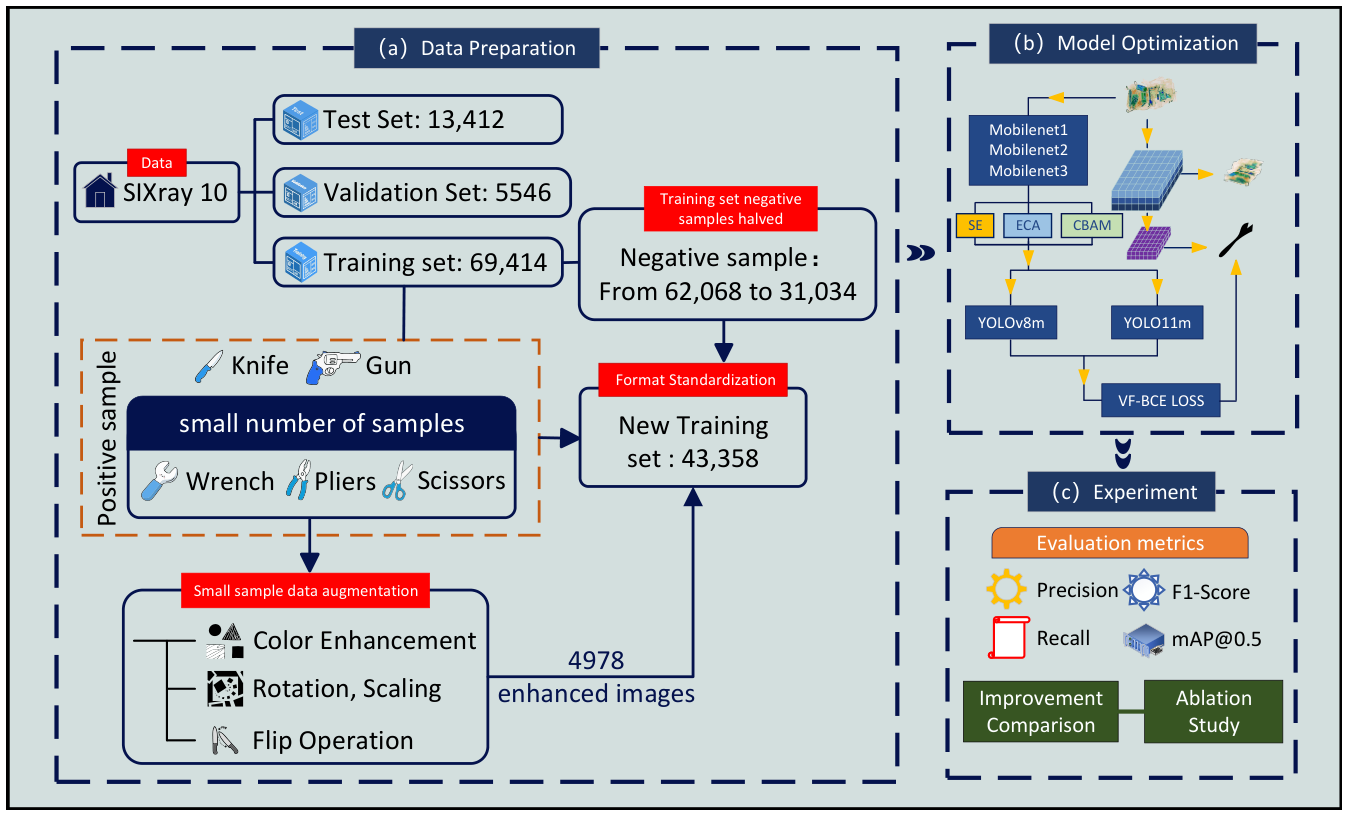
Figure 1 presents an overview of the data augmentation methods applied to the SIXray dataset. The original dataset did not include a dedicated validation set. To address this, we constructed a validation set by randomly sampling 5546 images from the original training set, which initially comprised 74,960 images in total. The remaining 69,414 images formed a new training set, while the original 13,412 images were retained as the test set to prevent data leakage.

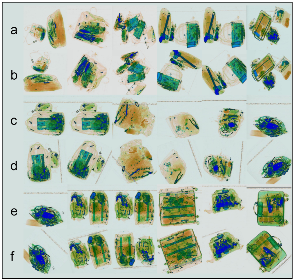
As shown in Figure 2, to mitigate the issue of insufficient sample size, images containing wrenches, pliers, and scissors were randomly rotated and scaled. The generated augmented samples were incorporated into the training set. After increasing the sample size for these three categories, the total number of training images reached 74,392. Since negative samples constituted over 85% of the dataset, potentially causing the model to favor “safe predictions,” the number of negative samples was halved to mitigate data bias, reducing the training set from 74,392 to 43,358 images. Unlike traditional methods that rely solely on oversampling or undersampling to adjust data distribution, this approach combines rotation-scaling augmentation with negative sample reduction. This optimizes the positive-to-negative sample ratio from 1:6 to 1:3, better accommodating complex scene requirements.

To evaluate data augmentation effectiveness, we compared the accuracy of two models on both the original and augmented datasets (

Table 1. Effect of data augmentation on the recognition precision of YOLOv8m and YOLO11m.

Model	Data	Gun	Knife	Wrench	Pliers	Scissors	Background
		(2495/3330)	(1625/2066)	(1532/3734)	(2956/6330)	(709/1490)	(62,068/31,034)
YOLOv8m	original-dataset	0.96223	0.94755	0.83846	0.85025	0.78019	0.97215
	data-augmented-dataset	0.95341	0.95341	0.84375	0.85079	0.79909	0.97010
YOLO11m	original-dataset	0.95699	0.91549	0.78153	0.85300	0.77283	0.96762
	data-augmented-dataset	0.97431	0.96014	0.79116	0.86043	0.77570	0.96657

Note: Numbers in parentheses indicate box counts (original/augmented).

).

As detailed in Table 1, the data augmentation strategy yielded a substantial surge in rare category instances. Specifically, initially scarce samples such as Scissors (increasing from 709 to 1490), Wrench (from 1532 to 3734), and Pliers experienced a twofold or greater increase. Concurrently, background samples were rigorously suppressed, plummeting from 62,068 to 31,034. This augmentation approach successfully rectified the extreme inherent data imbalance, effectively breaking the model’s bias towards background dominance and compelling it to extract features from historically rare contraband items. Observing the precision variations of YOLOv8m before and after augmentation, easily identifiable or majority classes experienced a marginal precision drop (e.g., Gun decreased from 0.96223 to 0.95341). Conversely, extremely challenging rare classes demonstrated notable gains, with Scissors improving from 0.78019 to 0.79909. For YOLOv8m, data augmentation served as a pivotal rebalancing mechanism. Sacrificing a negligible amount of precision in head classes to secure significant improvements in difficult tail classes constitutes a highly advantageous trade-off for real-world security screening scenarios. In contrast to YOLOv8m, YOLO11m exhibited exceptional performance post-augmentation: all foreground target classes (Gun, Knife, Wrench, Pliers, and Scissors) achieved positive precision growth. Most notably, the precision of Knife saw a dramatic leap from 0.91549 to 0.96014. Under this data-rebalancing protocol, the YOLO11m baseline accommodates the augmented training distribution more favorably than YOLOv8m for the reported foreground categories.

For the prohibited-item detection task considered in this study, Precision, Recall, F1-score, and mAP50 were selected as the core evaluation metrics. Precision, Recall, and F1-score summarize classification reliability under imbalanced conditions [23], while mAP50 evaluates the combined localization and classification quality at an intersection-over-union threshold of 0.5. Together, these metrics reflect the trade-off between false alarms, missed detections, and overall detection performance.

3.2. Scale-Aware MobileNetV3 Backbone Reconstruction

The computational capacity, memory bandwidth, and energy budget of edge-based X-ray inspection equipment are substantially lower than those of workstation GPUs. Direct deployment of a conventional YOLO backbone may therefore impose excessive storage and arithmetic costs, even when the detector satisfies the required recognition accuracy. To reduce this deployment burden, the original backbone is reconstructed using MobileNetV3-Small, while the neck and detection heads are retained so that the structural effect of backbone replacement can be evaluated independently.

MobileNet factorizes a standard convolution into channel-wise spatial filtering and pointwise channel mixing, thereby establishing an explicit trade-off between recognition accuracy and resource consumption [24]. This operator has subsequently been adopted in lightweight detection and structured compression frameworks to reduce the cost of feature extraction [25,26]. These studies also indicate that a reduction in theoretical FLOPs does not automatically guarantee an equivalent detector-level acceleration, because the interaction between depthwise and pointwise operations, memory access, and the target hardware must also be considered.

The preservation of information becomes more critical as model capacity decreases. MobileNetV2 introduced inverted residuals and linear bottlenecks because nonlinear transformations in narrow feature spaces may destroy information that cannot be recovered by subsequent layers [27]. MobileNetV3 further combined these principles with hardware-aware neural architecture search and NetAdapt-based platform adaptation, and separately optimized its Large and Small variants for different resource regimes [28,29]. Its hard-swish activation is intended as a hardware-oriented approximation of swish rather than an assertion of universally superior nonlinear representation [30]. The low arithmetic burden of MobileNetV3 has consequently motivated its use in power-constrained vision systems and lightweight YOLO detectors [31,32]. In the X-ray inspection domain, LightRay replaced the YOLOv4 backbone with MobileNetV3 and introduced shallow-feature enhancement and attention-based fusion to compensate for information loss affecting small and occluded targets [11]. These findings motivate the research sequence adopted here: the lightweight backbone is first evaluated as an isolated structural intervention, and attention-based compensation is then examined separately in Section 3.3.

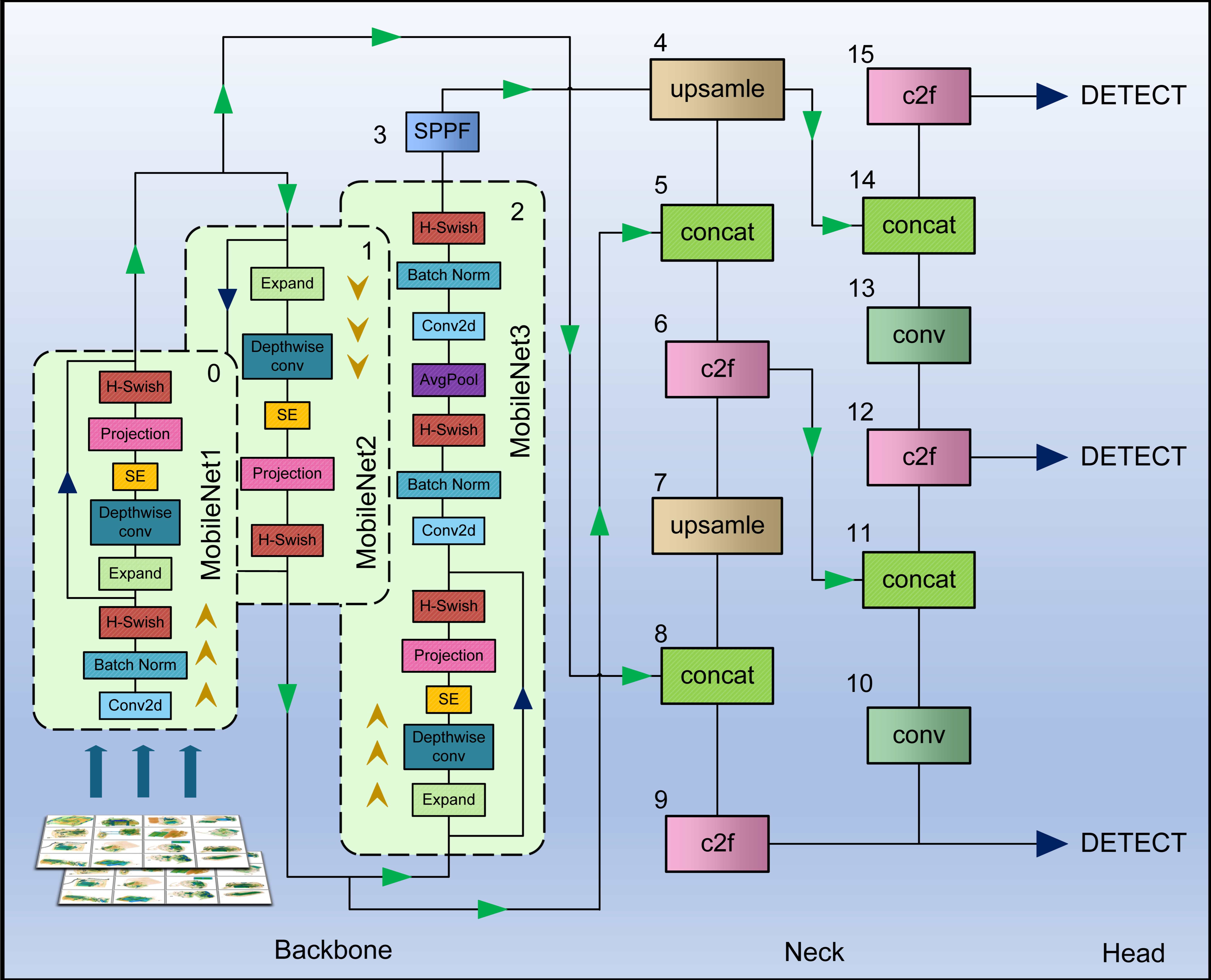
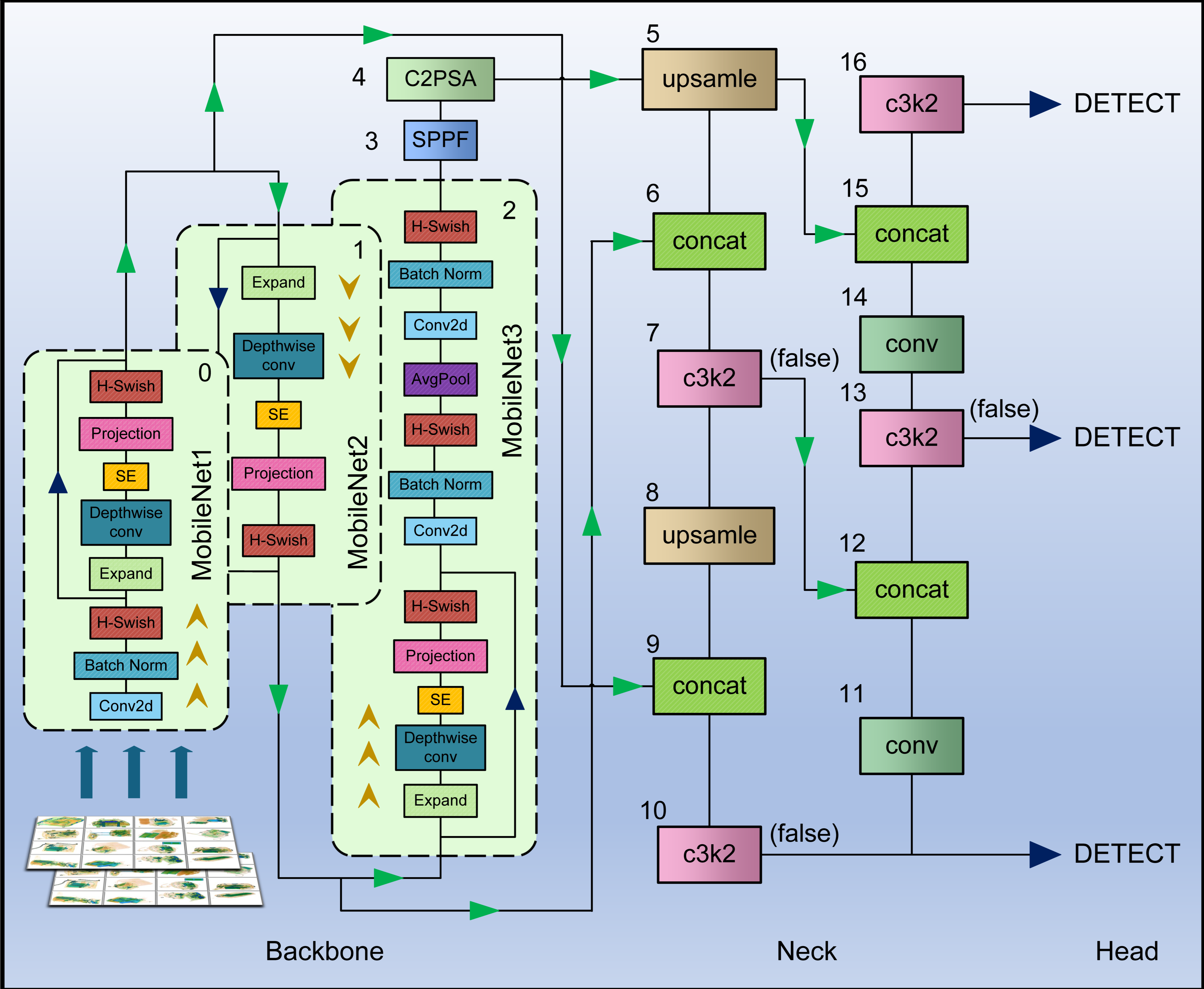
The detailed reconstruction paths are shown in Figure 3 and Figure 4. In the implemented YOLOv8m and YOLO11m definitions, the original backbone portion corresponding to layers 0–8 is replaced by three cascaded MobileNetV3-Small stages, denoted MobileNet1, MobileNet2, and MobileNet3. MobileNet1 extracts shallow, high-resolution features and routes them to the second concatenation path of the neck, located at layer 8 in Figure 3 and layer 9 in Figure 4. MobileNet2 produces intermediate features describing object shape and occlusion relationships and connects them to the first concatenation path, located at layer 5 in Figure 3 and layer 6 in Figure 4. MobileNet3 supplies the deep semantic representation to the original top-down and bottom-up feature-fusion path. The upsampling, concatenation, multiscale fusion, and detection-head structures are otherwise retained. This arrangement preserves three-level feature delivery while allowing the original convolutional stack to be replaced by inverted-residual and depthwise-separable operations.

To determine whether the same reconstruction behaves consistently at different detector capacities, the experiment was extended from the principal YOLO11m model to the n, s, and l variants. YOLOv8m is retained as a cross-generation reference. For every YOLO11 baseline–MobileNet pair, the data split, image resolution, optimization protocol, evaluation procedure, and random seed were held constant. All scale-wise results reported in

Table 2. Scale-wise comparison of the original and MobileNetV3-reconstructed detectors on the SIXray test set.

Family/Scale	Model	mAP50	Params	FLOPs	$\Delta$mAP50	$\Delta$Params	$\Delta$FLOPs
			(M)	(G)	(pp)	(%)	(%)
YOLOv8m	YOLOv8m	0.88009	33.940	85.400	–	–	–
	YOLOv8m-MobileNet	0.89615	20.070	67.700	+1.606	−40.87	−20.73
YOLO11n	YOLO11n	0.79751	2.591	6.445	–	–	–
	YOLO11n-MobileNet	0.78164	2.847	5.138	−1.587	+9.88	−20.28
YOLO11s	YOLO11s	0.83121	9.430	21.557	–	–	–
	YOLO11s-MobileNet	0.83254	6.580	11.635	+0.133	−30.22	−46.03
YOLO11m	YOLO11m	0.87235	20.030	67.300	–	–	–
	YOLO11m-MobileNet	0.88469	12.000	28.800	+1.234	−40.09	−57.21
YOLO11l	YOLO11l	0.90961	25.314	87.291	–	–	–
	YOLO11l-MobileNet	0.91258	15.258	38.298	+0.297	−39.73	−56.13

use random seed 41. The absolute change in mAP50 is reported in percentage points, while parameter and FLOP changes are calculated relative to the corresponding baseline.

Table 2 shows that the effect of MobileNetV3 reconstruction is scale dependent rather than uniformly beneficial. For YOLO11n, FLOPs decrease by 20.28%, but mAP50 decreases from 0.79751 to 0.78164, corresponding to a loss of 1.587 percentage points. The parameter count also increases from 2.591 M to 2.847 M. Thus, the adopted reconstruction does not constitute effective parameter compression at the n scale. Because the original nano model is already highly compact, the fixed cost of stage interfaces and channel adaptation occupies a larger fraction of the network, while the reduced cross-channel interaction of depthwise convolution becomes more consequential. The result is therefore treated as a capacity-limited failure case rather than being concealed as a successful lightweighting result. This interpretation is compatible with the information-preservation motivation behind the linear bottlenecks of MobileNetV2 [27]. YOLO11s occupies a more favorable operating region. Its mAP50 changes from 0.83121 to 0.83254, an increase of only 0.133 percentage points, while parameters and FLOPs decrease by 30.22% and 46.03%, respectively.

The strongest observed accuracy–efficiency result occurs at the m scale. YOLO11m-MobileNet improves mAP50 from 0.87235 to 0.88469 under seed 41, corresponding to a gain of 1.234 percentage points, while reducing parameters from 20.03 M to 12.00 M and FLOPs from 67.3 G to 28.8 G. Because YOLO11m was selected as the principal architecture, the baseline–MobileNet comparison was additionally repeated using seeds 42 and 43. As shown in

Table 3. Three-seed repeatability of the YOLO11m MobileNetV3 backbone-replacement experiment. The paired change is calculated between runs using the same random seed.

Model	Seed 41	Seed 42	Seed 43	Mean ± SD
YOLO11m	0.87235	0.87273	0.85829	0.86779 ± 0.00823
YOLO11m-MobileNet	0.88469	0.88583	0.87481	0.88178 ± 0.00606
Paired $\Delta$mAP50	+0.01234	+0.01310	+0.01652	+0.01399 ± 0.00223

, the MobileNetV3-reconstructed model improves mAP50 under all three evaluated seeds. The complete downstream module-ablation study was subsequently conducted using seeds 41, 42, and 43, following the statistical reporting protocol described in Section 4.1.3.

For YOLO11l, the parameter count and FLOPs decrease by 39.73% and 56.13%, respectively, whereas mAP50 rises by 0.297 percentage points. The l-scale model therefore retains sufficient absolute capacity after compression, and much of its original computation appears redundant for the present five-category SIXray task. However, the accuracy difference is small and has not yet been verified by repeated-seed experiments. In addition, the compressed l model still requires 15.258 M parameters and 38.298 G FLOPs, exceeding the cost of YOLO11m-MobileNet and weakening its suitability for constrained deployment.

The YOLOv8m comparison provides cross-generation evidence that MobileNet-based reconstruction can also preserve or improve detection performance outside the YOLO11 family. The reconstructed model increases mAP50 from 0.88009 to 0.89615, corresponding to a gain of 1.606 percentage points, while reducing the parameter count from 33.94 M to 20.07 M and FLOPs from 85.4 G to 67.7 G.

The observed non-monotonic pattern agrees with the broader model-scaling literature without being directly implied by it. EfficientNet demonstrated that depth, width, and input resolution should be balanced rather than changed independently [33]; EfficientDet extended this principle to the joint scaling of the backbone, feature-fusion network, and prediction heads in an object detector [34]. In the present experiment, the same MobileNetV3 reconstruction interacts with neck and head configurations of different capacities. At the n scale, the representational bottleneck and fixed interface overhead dominate; at the s scale, accuracy is maintained under compression; at the m scale, redundancy removal and retained capacity are most favorably balanced; and at the l scale, large computational redundancy can be removed, but the remaining deployment cost is still comparatively high.

Accordingly, MobileNetV3 should not be described as a universally beneficial drop-in replacement for every YOLO scale. The experiments instead identify a capacity-dependent operating range. YOLO11n approaches the lower representational boundary, YOLO11s offers accuracy-preserving compression, and YOLO11l retains unnecessary deployment cost despite strong compression. YOLO11m provides the most favorable observed balance among detection accuracy, parameter count, and arithmetic complexity, and the positive effect of its backbone reconstruction is reproduced across the three evaluated seeds. It is therefore selected as the principal YOLO11 architecture for the attention-compensation experiments in Section 3.3 and the subsequent VF-BCE optimization.

The scale-wise experiment above is a backbone-reconstruction study and should not be confused with the final-model comparison requested for lightweight deployment. A direct comparison of the complete YOLO-EMV model against the standard YOLO11n, YOLO11s, and YOLO11m baselines under the common seed-41 protocol is reported separately in Section 4.4.

3.3. Attention Mechanism for Enhanced Feature Extraction

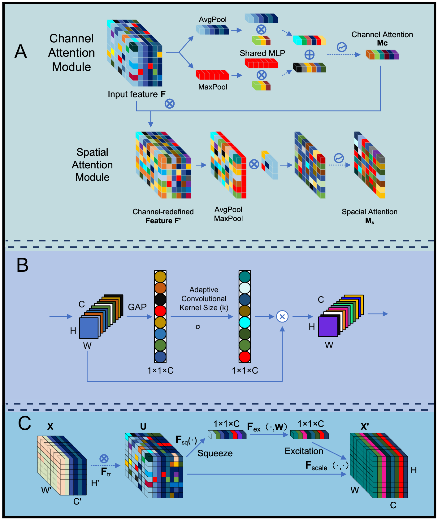
Complex X-ray scenes contain overlapping objects, low-contrast boundaries, and substantial background interference, which can weaken the detector response to small or partially occluded prohibited items [35,36,37]. Three representative attention mechanisms were therefore compared. CBAM combines sequential channel and spatial attention to refine feature responses [38]; SE models global channel dependencies through squeeze and excitation operations [39]; and ECA performs lightweight local cross-channel interaction using one-dimensional convolution without dimensionality reduction [40]. Their structures are summarized in Figure 5.

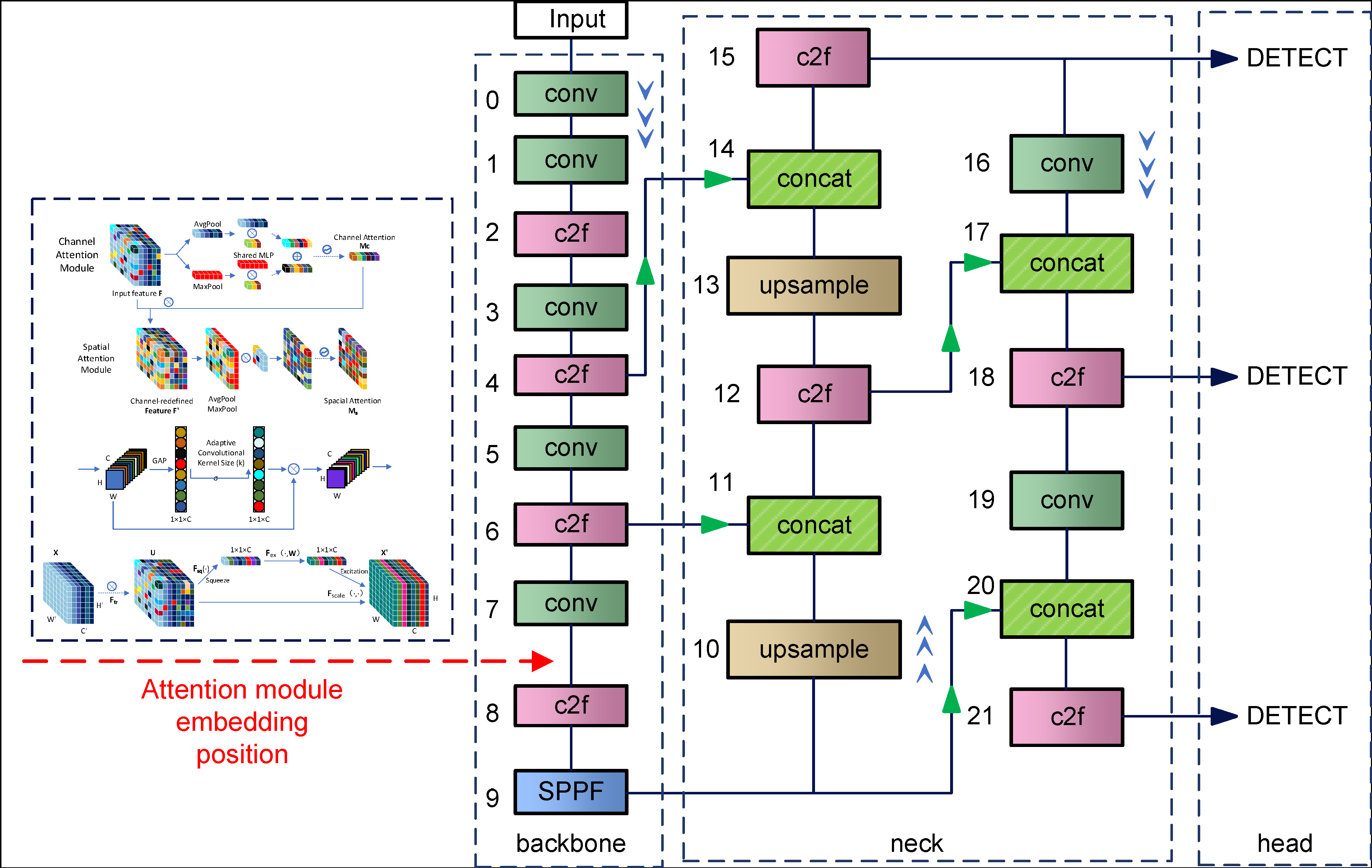
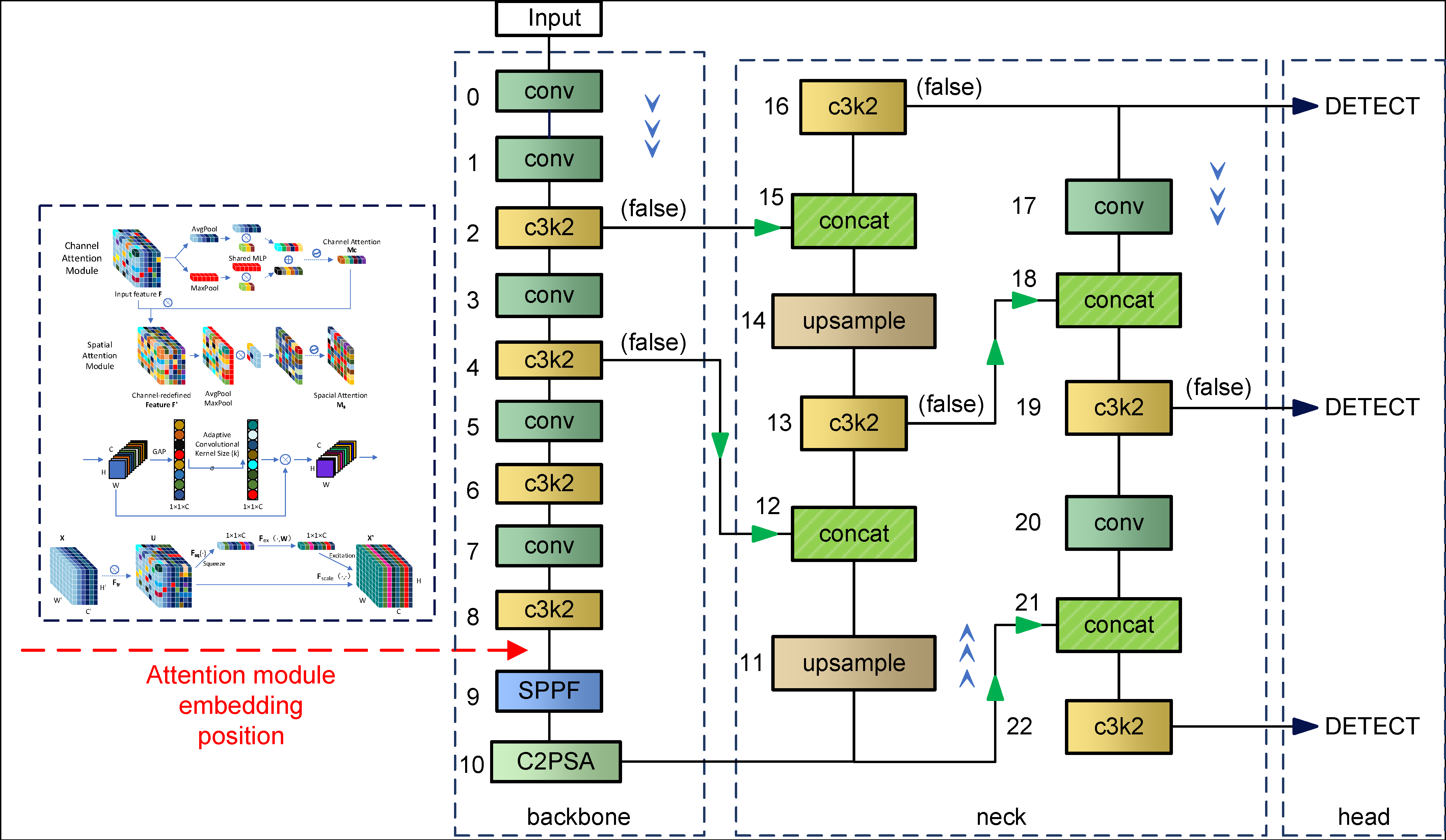
The three mechanisms were first screened on the original YOLOv8m and YOLO11m backbones under the unified seed-41 protocol. This screening stage was designed to compare the relative behavior of CBAM, SE, and ECA before the selected mechanisms were transferred to the corresponding lightweight feature pathways. In both baseline architectures, the candidate attention module was inserted after the eighth backbone block. At an input resolution of $640\times 640$, this position corresponds to a $20\times 20$ deep semantic feature map, allowing the attention candidates to be compared at the same feature level while leaving the neck and detection heads unchanged. Figure 6 and Figure 7 show the insertion points in YOLOv8m and YOLO11m, respectively.

All attention candidates were trained for 100 epochs using an input resolution of $640\times 640$, a batch size of 64, and an initial learning rate of 0.01. The learning rate, data partition, training schedule, baseline architecture, and evaluation procedure were held constant within each screening experiment so that the observed differences primarily reflected the selected attention mechanism.

As shown in

Table 4. Seed-41 attention-screening results for YOLOv8m on the SIXray test set.

YOLOv8m	mAP50	Params (M)	FLOPs (G)
Baseline	0.88009	33.94	85.4
+ CBAM	0.88275	34.53	85.8
+SE (selected)	0.89080	34.01	85.4
+ECA	0.87610	33.94	85.7

and

Table 5. Seed-41 attention-screening results for YOLO11m on the SIXray test set.

YOLO11m	mAP50	Params (M)	FLOPs (G)
Baseline	0.87235	20.03	67.3
+CBAM	0.88357	20.30	67.9
+SE	0.87511	20.07	67.7
+ECA (selected)	0.88505	20.03	67.9

, under seed 41, SE achieves the highest mAP50 among the YOLOv8m candidates, increasing mAP50 from 0.88009 to 0.89080. ECA achieves the highest mAP50 among the YOLO11m candidates, increasing mAP50 from 0.87235 to 0.88505. These single-seed tables are used for attention-candidate selection rather than for claims of run-to-run robustness. SE and ECA are subsequently integrated into the corresponding YOLO-SMV and YOLO-EMV lightweight pathways, and their interactions with MobileNetV3 and VF-BCE are evaluated in Section 4.2. In particular, the repeatability of the ECA contribution is assessed through the complete three-seed YOLO11m factorial ablation.

3.4. Class-Sensitive VF-BCE Loss Design and Parameter Selection

The SIXray training set presents two related optimization difficulties: a large number of background candidates relative to prohibited-item targets, and marked differences in recognition difficulty among the five prohibited-item categories. BCE provides stable binary classification supervision, but it does not explicitly reduce the accumulated contribution of easy negative samples. Focal Loss addresses this issue by down-weighting well-classified examples [41], while Varifocal Loss (VFL) further learns an IoU-aware classification score and applies asymmetric weighting to positive and negative samples [42]. These properties motivate the use of VFL for quality-aware and hard-sample optimization, with BCE retained as a complementary classification term.

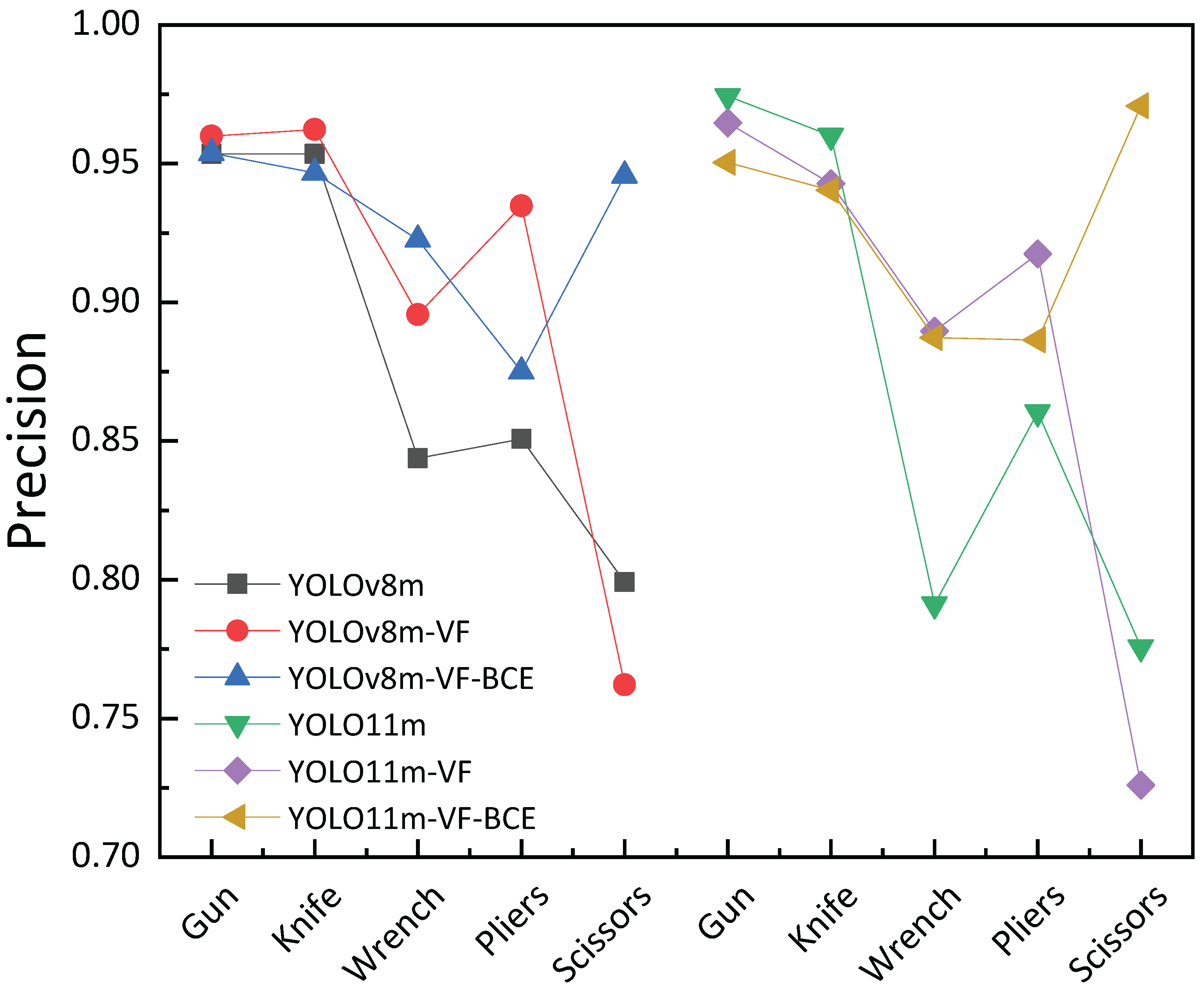
Before determining the fusion coefficient, the category-compensation strategy is fixed so that only the influence of $\beta$ is varied in the subsequent ablation. Class reweighting is a common approach to mitigating category imbalance [43]; however, direct inverse-frequency weighting is not adopted here because category frequency alone does not fully describe detection difficulty. On the augmented SIXray data, the YOLO11m BCE baseline obtains Precision values of 0.97431, 0.96014, 0.79116, 0.86040, and 0.77570 for Gun, Knife, Wrench, Pliers, and Scissors, respectively. Gun and Knife therefore retain unit weights; Wrench and Pliers receive moderate compensation because of their lower baseline performance; and Scissors receives the largest weight because it combines the lowest baseline Precision with the smallest augmented instance count among the five categories. The fixed weight vector is

$$\mathit{\omega }=[1.0,1.0,1.5,1.5,2.0],$$

(1)

corresponding to Gun, Knife, Wrench, Pliers, and Scissors. These weights remain unchanged in all $\beta$ experiments.

Following the original VFL formulation, the class-weighted VFL term used in this study is defined as

$${\mathcal{L}}_{\mathrm{VFL},c}=\left\{\begin{array}{cc}-{\omega }_c{q}_c\left[q_c\log \left(p_c\right)+(1-q_c)\log (1-p_c)\right],\hfill & q_c>0,\hfill \\ -{\omega }_c\alpha p_c^{\gamma }\log (1-p_c),\hfill & q_c=0,\hfill \end{array}\right.$$

(2)

where $p_c\in (0,1)$ is the predicted classification score and $q_c\in [0,1]$ is the IoU-aware target. For a matched positive sample, $q_c$ is the IoU between the predicted box and the corresponding ground-truth box; for a negative sample, $q_c=0$. The parameters $\alpha =0.75$ and $\gamma =2.0$ control negative-sample scaling and focusing strength, respectively. The total VFL term is

$${\mathcal{L}}_{\mathrm{VFL}}={\displaystyle \sum _{c=1}^K}{\mathcal{L}}_{\mathrm{VFL},c},$$

(3)

where $K=5$.

The BCE term is defined as

$${\mathcal{L}}_{\mathrm{BCE}}=-{\displaystyle \frac{1}{K}}{\displaystyle \sum _{c=1}^K}\left[y_c\log \left(p_c\right)+(1-y_c)\log (1-p_c)\right],$$

(4)

where $y_c\in \{0,1\}$ is the binary class label. The proposed composite loss is then written as

$${\mathcal{L}}_{\mathrm{VF}-\mathrm{BCE}}=\beta {\mathcal{L}}_{\mathrm{VFL}}+(1-\beta ){\mathcal{L}}_{\mathrm{BCE}},0\le \beta \le 1.$$

(5)

A linear mixing coefficient is also used in other compound-loss formulations to balance complementary supervision objectives [44]. In Equation (5), $\beta =0$ is exactly the BCE endpoint, whereas $\beta =1$ is the class-weighted VFL endpoint.

The expected influence of $\beta$ can be examined from the class-wise loss. For a positive sample ($q_c>0$ and $y_c=1$), Equation (5) becomes

$$\begin{array}{cc}\hfill {\mathcal{L}}_c^{+}=-& \left[\beta {\omega }_c{q}_c^2+{\displaystyle \frac{1-\beta }{K}}\right]\log \left(p_c\right)\hfill \\ \hfill -& \beta {\omega }_c{q}_c(1-q_c)\log (1-p_c).\hfill \end{array}$$

(6)

This can be interpreted as a scaled BCE with the effective target

$$t_c^{\mathrm{eff}}={\displaystyle \frac{\beta {\omega }_c{q}_c^2+(1-\beta )/K}{\beta {\omega }_c{q}_c+(1-\beta )/K}}.$$

(7)

Thus, $t_c^{\mathrm{eff}}=1$ at $\beta =0$, while $t_c^{\mathrm{eff}}\to q_c$ as $\beta \to 1$. Increasing $\beta$ therefore makes the classification score more strongly reflect localization quality. For a negative sample, the corresponding term is

$${\mathcal{L}}_c^{-}=-\left[\beta {\omega }_c\alpha p_c^{\gamma }+{\displaystyle \frac{1-\beta }{K}}\right]\log (1-p_c).$$

(8)

For an easy negative with $p_c\to 0$, this term approaches

$${\mathcal{L}}_c^{-}\approx -{\displaystyle \frac{1-\beta }{K}}\log (1-p_c),$$

(9)

showing that increasing $\beta$ progressively suppresses easy-background gradients. At the same time, the fixed category weights amplify the VFL term more strongly for Wrench and Pliers (${\omega }_c=1.5$) and Scissors (${\omega }_c=2.0$). For these categories, the nominal coefficients $\beta {\omega }_c$ are 1.05/1.40 at $\beta =0.7$, 1.20/1.60 at $\beta =0.8$, and 1.35/1.80 at $\beta =0.9$. Therefore, the principal search interval is set to $0.7\le \beta \le 0.9$: lower values may provide insufficient focusing, whereas values close to 1 may leave limited complementary BCE supervision. The two endpoints are retained to identify the effect of each single loss.

The fusion coefficient was screened under a controlled seed-41 protocol. All candidate values of $\beta$ were evaluated using the same random seed, data partition, training schedule, and evaluation procedure, so that between-seed variation did not confound the coefficient comparison. This table is therefore treated as a single-seed exploratory coefficient ablation rather than as a multi-seed robustness analysis. After fixing $\beta =0.8$, the selected VF-BCE configuration was subsequently evaluated using seeds 41, 42, and 43 as part of the complete factorial ablation in Section 4.2.

Accordingly, the following settings are evaluated on the YOLO11m baseline:

$$\beta \in \{0,0.7,0.8,0.9,1\}.$$

(10)

The class weights in Equation (1) are fixed in every experiment, and the remaining training configuration is kept unchanged to isolate the effect of the fusion coefficient.

As shown in

Table 6. Seed-41 exploratory ablation of the VF-BCE fusion coefficient on YOLO11m. All coefficient settings use the same random seed and experimental protocol. P denotes class-wise Precision. The settings $\beta =0$ and $\beta =1$ correspond to the BCE and class-weighted VFL endpoints, respectively.

$\mathit{\beta }$	Loss Setting	mAP50	Gun P	Knife P	Wrench P	Pliers P	Scissors P
0	BCE endpoint	0.87235	0.97431	0.96014	0.79116	0.86040	0.77570
0.7	VF-BCE	0.91926	0.95042	0.93386	0.96530	0.87424	0.94647
0.8	VF-BCE	0.92710	0.95044	0.94035	0.88732	0.88650	0.97087
0.9	VF-BCE	0.88917	0.96278	0.94189	0.88967	0.91096	0.75671
1	Class-weighted VFL endpoint	0.89262	0.96472	0.94283	0.88965	0.91745	0.72594

and Figure 8, the seed-41 mAP50 increases from 0.87235 at the BCE endpoint to 0.91926 at $\beta =0.7$, and reaches the maximum value of 0.92710 at $\beta =0.8$. Relative to the BCE and class-weighted VFL endpoints within this controlled single-seed comparison, the selected setting is higher by 5.475 and 3.448 percentage points, respectively. Increasing $\beta$ to 0.9 or 1 does not produce a further gain under the same seed, indicating that a larger VFL coefficient is not monotonically beneficial under the fixed class-weight scheme.

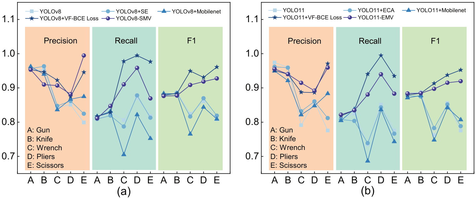
The category-level Precision values provide complementary evidence for this selection. The weighted categories respond differently to the fusion coefficient: Wrench reaches its highest seed-41 Precision at $\beta =0.7$, whereas Scissors reaches its highest value at $\beta =0.8$. When $\beta$ rises to 0.9 and 1, Pliers continues to improve, but Scissors decreases to 0.75671 and 0.72594, respectively.

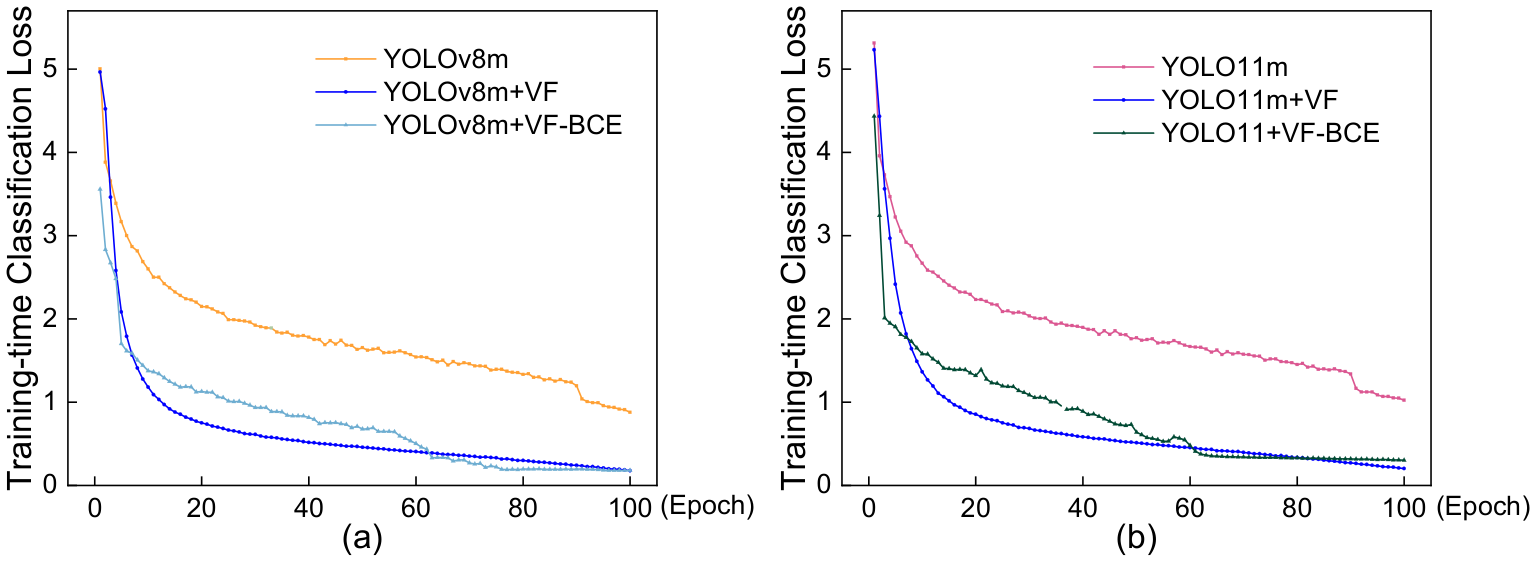
Figure 9 compares the classification-loss curves of the BCE, class-weighted VFL, and VF-BCE variants during training. All three settings exhibit stable within-objective convergence. Because BCE, VFL, and VF-BCE use different sample-weighting mechanisms and therefore have different numerical scales, neither their absolute magnitudes nor their apparent decay rates are directly comparable. The curves are consequently used only to examine optimization stability within each loss setting; the selected VF-BCE configuration shows no evident oscillatory behavior during training.

4. Results

4.1. Datasets, Implementation Details, and Reporting Protocol

4.1.1. Datasets

All experiments on SIXray used the same training, validation, and test partitions described in Section 3.1. The augmented training set was used throughout the subsequent module comparisons so that differences between configurations could be attributed to the evaluated architectural or loss-function changes rather than to changes in the data distribution. OPIXray and PIDray were used only in the external-validation experiments described in the corresponding subsections.

4.1.2. Implementation Details

The experiments were implemented in Python 3.8 using PyTorch 2.0.0, CUDA 11.8, and the Ultralytics detection framework. Training was conducted on a workstation equipped with two NVIDIA GeForce RTX 4090D GPUs, each with 24 GB of memory, and an AMD EPYC 9754 processor with 128 physical cores and 256 threads. The operating system was Ubuntu 20.04.

Unless otherwise stated, the principal YOLOv8m and YOLO11m experiments were trained for 100 epochs with an input resolution of $640\times 640$ pixels and a batch size of 64. The YOLO11l scale experiment used a batch size of 32 because of its higher memory demand. SGD was used with a momentum of 0.937 and a weight decay of 0.0005. Experiment-specific learning-rate settings are reported in the corresponding methodological subsections rather than treated as a single global value. Within each controlled comparison, the data split, augmentation protocol, optimization settings, evaluation procedure, and test set were kept unchanged.

4.1.3. Random-Seed Protocol and Statistical Reporting

The complete factorial module-ablation study on YOLO11m was independently conducted using random seeds 41, 42, and 43. For these experiments, mAP50 is reported as the mean and sample standard deviation over the three runs. Performance changes were first calculated separately between configurations trained with the same random seed. The reported $\Delta$mAP50 therefore represents the mean and sample standard deviation of paired, within-seed differences.

YOLOv8m was retained as a cross-generation auxiliary validation model and was evaluated using seed 41. The YOLO11n, YOLO11s, and YOLO11l scale-wise comparisons were also conducted using a unified single-seed protocol. These single-seed results are interpreted descriptively and are not used to support claims of run-to-run statistical robustness. Parameter counts and FLOPs are deterministic properties of the inference architecture and are therefore reported once for each configuration rather than as multi-run statistics.

4.2. Multi-Seed Ablation on YOLO11m and Auxiliary Validation on YOLOv8m

Following the protocol defined in Section 4.1.3, the principal ablation study was performed on YOLO11m using all eight combinations of ECA, MobileNetV3, and VF-BCE. YOLOv8m was retained as a single-seed auxiliary model to examine whether the same qualitative interaction pattern also appears in an earlier YOLO generation. The two result groups therefore serve different purposes: the YOLO11m experiments support the main repeatability analysis, whereas the YOLOv8m experiments provide descriptive cross-generation evidence.

As shown in

Table 7. Three-seed factorial ablation results for YOLO11m on the SIXray test set. The seed-wise mAP50 values are provided in Appendix A Table A1.

Baseline	ECA	MobileNetV3	VF-BCE	mAP50	$\Delta$mAP50	Params	FLOPs
				Mean ± SD	Mean ± SD (pp)	(M)	(G)
✓				$0.86779\pm 0.00823$	–	20.03	67.3
✓	✓			$0.88118\pm 0.00610$	$+1.339\pm 0.221$	20.03	67.9
✓		✓		$0.88178\pm 0.00606$	$+1.399\pm 0.223$	12.00	28.8
✓			✓	$0.92258\pm 0.00743$	$+5.479\pm 0.090$	20.03	67.3
✓	✓	✓		$0.89269\pm 0.00704$	$+2.490\pm 0.123$	12.04	28.8
✓	✓		✓	$0.93842\pm 0.00720$	$+7.063\pm 0.108$	20.03	67.9
✓		✓	✓	$0.90636\pm 0.00571$	$+3.857\pm 0.253$	12.00	28.8
✓	✓	✓	✓	$0.92744\pm 0.00768$	$+5.965\pm 0.093$	12.04	28.8

, the original YOLO11m achieves an average mAP50 of $0.86779\pm 0.00823$. When evaluated individually, ECA and MobileNetV3 provide mean paired gains of $1.339\pm 0.221$ and $1.399\pm 0.223$ percentage points, respectively. VF-BCE produces the largest individual improvement, increasing mAP50 by $5.479\pm 0.090$ percentage points. The positive within-seed changes observed for all three individual modules indicate that the direction of improvement is consistent across the evaluated initializations.

The highest average detection accuracy is obtained by the ECA+VF-BCE configuration, which reaches $0.93842\pm 0.00720$. This result identifies ECA+VF-BCE as the accuracy-oriented configuration. The complete YOLO-EMV model achieves a lower mAP50 of $0.92744\pm 0.00768$, but it still improves upon the original YOLO11m by $5.965\pm 0.093$ percentage points while reducing the parameter count from 20.03 M to 12.04 M and FLOPs from 67.3 G to 28.8 G. These changes correspond to reductions of 39.9% and 57.2%, respectively. YOLO-EMV is therefore interpreted as the deployment-oriented configuration rather than as the configuration with the highest absolute accuracy.

The paired module comparisons further clarify the compression–compensation relationship. Replacing the original backbone with MobileNetV3 and then applying VF-BCE yields an average mAP50 of $0.90636\pm 0.00571$, which is $1.622\pm 0.182$ percentage points lower than applying VF-BCE to the uncompressed backbone. Adding ECA to the MobileNetV3+VF-BCE configuration increases mAP50 by $2.108\pm 0.214$ percentage points, producing the complete YOLO-EMV model. ECA therefore provides a repeatable compensatory contribution after lightweight reconstruction, although it does not completely eliminate the accuracy difference between the complete model and the uncompressed ECA+VF-BCE configuration. Indeed, YOLO-EMV remains $1.098\pm 0.061$ percentage points below ECA+VF-BCE, in exchange for substantially lower inference complexity.

The same results also show that the three modules are not simply additive. ECA improves the original baseline and also improves the compressed MobileNetV3 pathway, whereas the magnitude of its contribution depends on the accompanying loss and backbone configuration. Similarly, VF-BCE is the dominant source of accuracy improvement, but the lightweight backbone changes the capacity available for learning the strongly reweighted hard samples. The final architecture therefore reflects a controlled trade-off among feature capacity, channel recalibration, hard-sample optimization, and deployment cost.

The auxiliary YOLOv8m results in

Table 8. Auxiliary single-seed ablation results for YOLOv8m on the SIXray test set. All configurations were evaluated using seed 41.

Baseline	SE	MobileNetV3	VF-BCE	mAP50	$\Delta$mAP50	Params	FLOPs
					(pp)	(M)	(G)
✓				0.88009	–	33.94	85.4
✓	✓			0.89080	+1.071	34.01	85.4
✓		✓		0.89615	+1.606	20.07	67.7
✓			✓	0.92872	+4.863	33.94	85.4
✓	✓	✓		0.90343	+2.334	20.14	68.1
✓	✓		✓	0.93856	+5.847	34.01	85.4
✓		✓	✓	0.90867	+2.858	20.07	67.7
✓	✓	✓	✓	0.92929	+4.920	20.14	68.1

exhibit a qualitatively similar pattern. Under seed 41, SE+VF-BCE achieves the highest mAP50 of 0.93856, whereas the complete YOLO-SMV model obtains 0.92929 with substantially lower inference complexity. Relative to the original YOLOv8m, YOLO-SMV improves mAP50 by 4.920 percentage points while reducing the parameter count from 33.94 M to 20.14 M and FLOPs from 85.4 G to 68.1 G, corresponding to reductions of 40.7% and 20.3%, respectively.

4.3. Impact of Various Improved Modules on Different Categories of Prohibited Items

To examine class-specific behavior, Precision, Recall, and F1-score were compared across Gun, Knife, Wrench, Pliers, and Scissors. The category-level values in this subsection and in Appendix A 

Table A3. Comparison of detection metrics for the representative seed-41 YOLOv8m runs under individual and mixed improvement schemes. These values are not multi-seed averages. F1 scores are calculated from the Precision and Recall values in the same table using $F1=2PR/(P+R)$.

Model	Gun	Knife	Wrench	Pliers	Scissors
Precision
YOLOv8m	0.95341	0.95341	0.84375	0.85079	0.79909
YOLOv8m+SE	0.95676	0.96337	0.84739	0.86184	0.82465
YOLOv8m+MobileNet	0.96230	0.94014	0.83628	0.86704	0.87500
YOLOv8m+VF-BCE Loss	0.95374	0.94662	0.92254	0.87500	0.94570
YOLO-SMV	0.95341	0.90970	0.90706	0.88163	0.99465
Recall
YOLOv8m	0.81098	0.82866	0.80597	0.87131	0.81776
YOLOv8m+SE	0.80945	0.81932	0.78731	0.87802	0.81308
YOLOv8m+MobileNet	0.81707	0.83178	0.70522	0.82172	0.75234
YOLOv8m+VF-BCE Loss	0.81707	0.82866	0.97761	0.99464	0.97664
YOLO-SMV	0.81098	0.84735	0.91045	0.95845	0.86916
F1
YOLOv8m	0.87644	0.88667	0.82443	0.86093	0.80831
YOLOv8m+SE	0.87696	0.88552	0.81625	0.86985	0.81882
YOLOv8m+MobileNet	0.88375	0.88265	0.76518	0.84377	0.80905
YOLOv8m+VF-BCE Loss	0.88013	0.88372	0.94928	0.93099	0.96092
YOLO-SMV	0.87644	0.87742	0.90875	0.91843	0.92768

and

Table A4. Comparison of detection metrics for the representative seed-41 YOLO11m runs under individual and mixed improvement schemes. These values are not multi-seed averages. F1 scores are calculated from the Precision and Recall values in the same table using $F1=2PR/(P+R)$.

Model	Gun	Knife	Wrench	Pliers	Scissors
Precision
YOLO11m	0.97431	0.96015	0.79117	0.86043	0.77570
YOLO11m+ECA	0.96188	0.95911	0.83193	0.86047	0.81188
YOLO11m+MobileNet	0.94964	0.92123	0.82143	0.84783	0.88333
YOLO11m+VF-BCE Loss	0.95044	0.94035	0.88732	0.88650	0.97087
YOLO-EMV	0.95557	0.94035	0.94472	0.89186	0.95939
Recall
YOLO11m	0.80945	0.82555	0.73508	0.85121	0.77570
YOLO11m+ECA	0.80793	0.80374	0.73881	0.84316	0.76636
YOLO11m+MobileNet	0.80488	0.83801	0.68657	0.83646	0.74299
YOLO11m+VF-BCE Loss	0.81806	0.83489	0.94030	0.99464	0.93458
YOLO-EMV	0.82765	0.83489	0.88060	0.93968	0.88318
F1
YOLO11m	0.88426	0.88777	0.76209	0.85580	0.77570
YOLO11m+ECA	0.87821	0.87458	0.78261	0.85173	0.78846
YOLO11m+MobileNet	0.87129	0.87765	0.74797	0.84211	0.80711
YOLO11m+VF-BCE Loss	0.87930	0.88449	0.91304	0.93746	0.95238
YOLO-EMV	0.88702	0.88449	0.91153	0.91514	0.91971

correspond to the representative seed-41 runs and are not multi-seed averages. Figure 10 visualizes the YOLO11m variants, while the appendix tables provide the complete YOLOv8m and YOLO11m results.

For YOLOv8m, VF-BCE increases Precision for the weighted categories Wrench and Scissors from 0.84375 and 0.79909 to 0.92254 and 0.94570, respectively. The complete YOLO-SMV model obtains Precision values of 0.90706, 0.88163, and 0.99465 for Wrench, Pliers, and Scissors, although Knife Precision decreases from 0.95341 in the baseline to 0.90970. Thus, the class-specific changes are favorable for several difficult categories but are not uniformly positive across all classes.

For YOLO11m, VF-BCE increases Precision for Wrench, Pliers, and Scissors from 0.79117, 0.86043, and 0.77570 to 0.88732, 0.88650, and 0.97087, respectively. The complete YOLO-EMV model further raises Wrench and Pliers Precision to 0.94472 and 0.89186, while Scissors Precision remains high at 0.95939. Gun and Knife Precision are slightly lower than those of the original YOLO11m, indicating an accuracy redistribution rather than a uniform improvement for every category.

The Recall and F1-score results show a similar trade-off. Both complete models improve the difficult-category Recall and F1-score relative to their corresponding baselines, but the relative ranking between YOLO-SMV and YOLO-EMV depends on the metric. Across the five categories, YOLO-EMV has a higher macro-averaged Precision (0.93838 versus 0.92929) and a slightly higher macro-averaged F1-score (0.90358 versus 0.90174), whereas YOLO-SMV has a higher macro-averaged Recall (0.87928 versus 0.87320).

Figure 11 presents representative qualitative comparisons in the order YOLOv8m, YOLO-SMV, YOLO11m, and YOLO-EMV. The changes are not uniformly positive for every predicted box. For the top-left knife, the confidence increases from 0.86 to 0.87 and from 0.83 to 0.91 in the two model families, respectively. For the lower-left wrench, the corresponding confidence increases from 0.81 to 0.85 and from 0.75 to 0.78.

The lower-right example provides a clearer missed-detection comparison. YOLOv8m does not detect the gun, whereas YOLO-SMV recovers it with a confidence of 0.61. YOLO11m detects the same gun with a confidence of 0.54, while YOLO-EMV increases the confidence to 0.85. In the heavily overlapped gun scene in the upper-right part of the figure, the models retain different sets of overlapping detections. Consequently, some confidence values increase whereas others remain unchanged or decrease slightly, and the individual boxes cannot always be matched one-to-one. The figure is therefore used only as qualitative illustration. The overall performance conclusions are based on the complete test-set mAP50, Precision, Recall, and F1-score results.

4.4. Direct Comparison with Standard Lightweight YOLO Variants

The scale-aware reconstruction study in Section 3.2 asks whether the same compression operation behaves consistently across detector capacities. Here, the question is more directly deployment-oriented: why use the proposed medium-derived configuration instead of simply selecting a standard nano or small detector? Table 9 therefore compares the standard YOLO11n/s/m baselines with two operating points identified by the factorial study. All entries use the common seed-41 SIXray split, input resolution, and evaluation procedure so that accuracy and complexity can be interpreted within a single controlled setting.

Figure 11. Representative qualitative comparisons between each baseline and its complete deployment-oriented model: (A) YOLOv8m vs. YOLO-SMV; (B) YOLO11m vs. YOLO-EMV.

Figure 11. Representative qualitative comparisons between each baseline and its complete deployment-oriented model: (A) YOLOv8m vs. YOLO-SMV; (B) YOLO11m vs. YOLO-EMV.

Table 9. Direct seed-41 comparison of standard YOLO11 nano, small, and medium baselines with the accuracy-oriented and deployment-oriented operating points identified in this study. All models use the common SIXray experimental protocol.

Model/Operating Point	mAP50 (Seed 41)	Params (M)	FLOPs (G)
YOLO11n	0.79751	2.591	6.445
YOLO11s	0.83121	9.430	21.557
YOLO11m	0.87235	20.030	67.300
ECA+VF-BCE (accuracy-oriented)	0.94271	20.030	67.900
YOLO-EMV (deployment-oriented)	0.93240	12.040	28.800

Table 9. Direct seed-41 comparison of standard YOLO11 nano, small, and medium baselines with the accuracy-oriented and deployment-oriented operating points identified in this study. All models use the common SIXray experimental protocol.

Model/Operating Point	mAP50 (Seed 41)	Params (M)	FLOPs (G)
YOLO11n	0.79751	2.591	6.445
YOLO11s	0.83121	9.430	21.557
YOLO11m	0.87235	20.030	67.300
ECA+VF-BCE (accuracy-oriented)	0.94271	20.030	67.900
YOLO-EMV (deployment-oriented)	0.93240	12.040	28.800

The results show why the deployment problem cannot be reduced to selecting the smallest baseline. Relative to YOLO11s, YOLO-EMV uses moderately more computation but increases mAP50 by 10.119 percentage points under the same protocol. Relative to YOLO11m, it increases mAP50 by 6.005 percentage points while reducing parameters by 39.9% and FLOPs by 57.2%. The accuracy-oriented ECA+VF-BCE configuration reaches 0.94271 under seed 41, but retaining the original backbone keeps its complexity at 20.03 M parameters and 67.9 G FLOPs. YOLO-EMV therefore represents a deliberate movement away from the absolute-accuracy operating point: under seed 41 it gives up 1.031 percentage points relative to ECA+VF-BCE while reducing parameters by 39.9% and FLOPs by 57.6%. The corresponding three-seed comparison in Table 7 shows the same interpretation, with a mean accuracy difference of $1.098\pm 0.061$ percentage points. Thus, the principal claim is not that YOLO-EMV is the smallest detector, but that the medium-scale starting point permits a substantially different accuracy–efficiency operating point from the standard nano/small alternatives.

4.5. Protocol-Aware Comparison with Previously Published SIXray Results

The reviewer requested comparison with results reported in prior publications on the same public benchmark. We therefore reproduce representative published SIXray results in

Table 10. Protocol-aware comparison with representative previously published SIXray results. Source-reported values are reproduced from the cited publications. Dataset-processing and training settings are listed for each row because the effective SIXray protocols differ substantially across studies. The numerical values are therefore not interpreted as a controlled cross-paper ranking.

Study	Model	SIXray Data Used	Train/Val/Test Setting	Background/Negative Handling	Training Setting	mAP50
Wang et al. [13]	YOLOv8n	SIXray; exact image counts not explicitly reported	Not explicitly reported	Number of background-only images not explicitly reported	300 epochs; Mosaic; MixUp; horizontal flip; scale augmentation	0.908
Wang et al. [13]	YOLOv8s	SIXray; exact image counts not explicitly reported	Not explicitly reported	Number of background-only images not explicitly reported	300 epochs; Mosaic; MixUp; horizontal flip; scale augmentation	0.940
Wang et al. [13]	YOLOv8n-GEMA	SIXray; exact image counts not explicitly reported	Not explicitly reported	Number of background-only images not explicitly reported	300 epochs; Mosaic; MixUp; horizontal flip; scale augmentation	0.944
Zhao et al. [14]	YOLO11n	8929 manually annotated prohibited-item images	8:1:1 split of the 8929 images	Original million-scale negative pool not reported as included in the experimental subset	$640\times 640$; 600 epochs; scratch; SGD; batch 64; Mosaic+MixUp	0.923
Zhao et al. [14]	YOLO11s	8929 manually annotated prohibited-item images	8:1:1 split of the 8929 images	Original million-scale negative pool not reported as included in the experimental subset	$640\times 640$; 600 epochs; scratch; SGD; batch 64; Mosaic+MixUp	0.934
Zhao et al. [14]	Xray-YOLO-Mamba	8929 manually annotated prohibited-item images	8:1:1 split of the 8929 images	Original million-scale negative pool not reported as included in the experimental subset	$640\times 640$; 600 epochs; scratch; SGD; batch 64; Mosaic+MixUp	0.940
This study	YOLO11n	43,358 final training images; 5546 validation images; original 13,412-image test set retained	43,358/5546/13,412	31,034 background images retained after negative-sample reduction	$640\times 640$; 100 epochs; SGD; batch 64; seed 41	0.79751
This study	YOLO11s	43,358 final training images; 5546 validation images; original 13,412-image test set retained	43,358/5546/13,412	31,034 background images retained after negative-sample reduction	$640\times 640$; 100 epochs; SGD; batch 64; seed 41	0.83121
This study	YOLO11m	43,358 final training images; 5546 validation images; original 13,412-image test set retained	43,358/5546/13,412	31,034 background images retained after negative-sample reduction	$640\times 640$; 100 epochs; SGD; batch 64; seed 41	0.87235
This study	YOLO-EMV	43,358 final training images; 5546 validation images; original 13,412-image test set retained	43,358/5546/13,412	31,034 background images retained after negative-sample reduction	$\mathbf{640}\mathbf{\times }\mathbf{640}$; 100 epochs; SGD; batch 64; seeds 41/42/43	$\mathbf{0.92744}\pm \mathbf{0.00768}$

. However, the term “SIXray” does not necessarily correspond to an identical effective benchmark across publications. Different studies select different subsets from the original dataset, adopt different train–validation–test partitions, retain or omit different numbers of background-only images, and use substantially different training schedules and augmentation strategies. These differences affect the statistical composition and difficulty of the evaluated detection task. For this reason, Table 10 reports the available dataset-processing and training settings together with the reported mAP50, rather than presenting the numerical values as a common leaderboard.

Wang et al. [13] evaluated YOLOv8n, YOLOv8s, and YOLOv8n-GEMA on SIXray and reported mAP50 values of 0.908, 0.940, and 0.944, respectively. Their models were trained for 300 epochs and used Mosaic, MixUp, horizontal flipping, and scale augmentation. The publication does not explicitly report the SIXray train/validation/test image counts or the number of background-only images retained in the SIXray experiments; these fields are therefore identified as not explicitly reported rather than inferred.

Zhao et al. [14] define their SIXray experimental data as 8929 manually annotated images of prohibited items and divide these images into training, validation, and testing sets at an 8:1:1 ratio. Their models are trained from scratch for 600 epochs at an input resolution of $640\times 640$, using SGD with a batch size of 64 together with Mosaic and MixUp augmentation. The reported experimental description does not state that the original million-scale negative-image pool is incorporated into this 8929-image experimental subset. Under this protocol, YOLO11n and YOLO11s achieve mAP50 values of 0.923 and 0.934, respectively, and Xray-YOLO-Mamba reaches 0.940.

The protocol used in the present study is different. The original SIXray training partition contains 74,960 images. We randomly select 5546 images from this partition to construct the validation set and retain the original 13,412-image test set unchanged. After class-targeted augmentation and negative-sample reduction, the final training set contains 43,358 images, including 31,034 background images. The principal experiments use an input resolution of $640\times 640$, 100 training epochs, SGD, and a batch size of 64. The YOLO11n/s/m direct comparison uses seed 41, whereas the final YOLO-EMV result is reported over seeds 41, 42, and 43.

The differences summarized in Table 10 are not minor implementation details. They alter the effective data distribution on which the detector is trained and evaluated. In particular, Zhao et al. [14] construct their SIXray experiments from 8929 manually annotated prohibited-item images and repartition that subset at an 8:1:1 ratio. By contrast, the present study retains the original 13,412-image test set and preserves 31,034 background images in the final training set even after negative-sample reduction. The two studies therefore differ in the number of training and test images, foreground–background composition, training duration, and augmentation protocol. We do not infer from these differences that one protocol is intrinsically more difficult, nor do we attribute the performance gap to a single factor such as negative-image handling. The appropriate conclusion is that the source-reported values are produced under different experimental conditions.

The magnitude of this protocol dependence can be observed from nominally identical lightweight baseline scales. Zhao et al. [14] report mAP50 values of 0.923 and 0.934 for YOLO11n and YOLO11s, whereas the same nominal model scales obtain 0.79751 and 0.83121 under the protocol used in this study. The corresponding differences are 12.549 and 10.279 percentage points. These differences are much larger than the apparent cross-paper difference between Xray-YOLO-Mamba (0.940 in the same study) and YOLO-EMV ($0.92744\pm 0.00768$ in this study). This observation does not establish which proposed detector is intrinsically superior; instead, it shows that absolute source-reported SIXray mAP50 is strongly protocol dependent and should not be interpreted without the associated data-processing conditions.

Accordingly, Table 10 is used for contextual comparison rather than for a superiority ranking. It documents the performance range reported in representative recent SIXray studies and, at the same time, makes the associated experimental conditions visible. Direct claims regarding model improvement, parameter reduction, FLOP reduction, and the position of YOLO-EMV relative to nano, small, and medium YOLO baselines are based exclusively on the matched experiments conducted within this study in Table 2, Table 7, and Table 9. The separately controlled re-evaluation in Section 4.6 provides an additional head-to-head comparison under the fixed protocol adopted here.

4.6. Controlled Re-Evaluation of Representative Public Detectors

To complement the source-reported literature comparison, three representative publicly available detectors were re-evaluated using the same SIXray training, validation, and held-out test partitions adopted in this study. YOLOv8-L+CSPDarkNet53 provides a high-capacity convolutional reference, YOLOv8-L+CHR provides an X-ray-specific CNN reference derived from the CHR design family evaluated in the recent comparative literature [15], and D-FINE-S provides a recent lightweight Transformer/DETR-family reference [45]. Architecture-specific implementations were retained, while the common data split, input resolution, and evaluation procedure were held fixed. Consequently, the mAP50 values in

Table 11. Controlled re-evaluation of representative public detectors on the held-out SIXray test set using the common data partition and evaluation protocol adopted in this study. The YOLO-EMV result is the mean ± sample standard deviation over seeds 41, 42, and 43; the external detector entries are the completed unified evaluation runs.

Configuration	Unified mAP50	Params (M)	GFLOPs
YOLOv8-L+CSPDarkNet53	0.90614	43.61	164.8
YOLOv8-L+CHR	0.87325	37.91	102.3
D-FINE-S	0.91237	10.20	25.2
YOLO-EMV (Ours)	$0.92744\pm 0.00768$	12.04	28.8

can be used for direct comparison within this study.

Within these completed unified runs, YOLO-EMV achieves a three-seed mean mAP50 of $0.92744\pm 0.00768$, exceeding the YOLOv8-L+CSPDarkNet53, YOLOv8-L+CHR, and D-FINE-S runs by 2.130, 5.419, and 1.507 percentage points, respectively. The comparison also exposes the intended trade-off rather than a universal dominance claim. YOLO-EMV is far less costly than the two large CNN references, whereas D-FINE-S is slightly smaller in absolute complexity (10.20 M parameters and 25.2 GFLOPs versus 12.04 M and 28.8 GFLOPs) but obtains lower mAP50 under the common evaluation. These matched results provide the basis for direct quantitative statements in this study; the heterogeneous source-reported values in Table 10 are used only as literature context.

4.7. Validation on the OPIXray Dataset

OPIXray is a benchmark for occluded prohibited-item detection in X-ray security inspection. It contains 8885 high-resolution images covering five controlled-knife categories: folding knife (1,993), straight knife (1044), scissors (1863), utility knife (1978), and multi-tool knife (2042). The dataset is divided into training and test sets at an approximately 4:1 ratio, and its heavily occluded samples provide a complementary setting to SIXray.

To examine whether the module-interaction patterns observed on SIXray also appear on a different X-ray benchmark, additional ablation experiments were conducted on OPIXray, with the results reported in

Table 12. Single-seed factorial ablation of SE, MobileNetV3, and VF-BCE on OPIXray using YOLOv8m.

Baseline	SE	MobileNetV3	VF-BCE	mAP50	Params(M)	FLOPs(G)
✓				0.87620	33.94	85.4
✓	✓			0.88139	34.01	85.4
✓		✓		0.85954	20.07	67.7
✓			✓	0.88396	33.94	85.4
✓	✓	✓		0.87159	20.14	68.1
✓	✓		✓	0.89276	34.01	85.4
✓		✓	✓	0.84915	20.07	67.7
✓	✓	✓	✓	0.86953	20.14	68.1

Note: A checkmark indicates that the corresponding component is included in the model configuration.

and

Table 13. Single-seed factorial ablation of ECA, MobileNetV3, and VF-BCE on OPIXray using YOLO11m.

Baseline	ECA	MobileNetV3	VF-BCE	mAP50	Params(M)	FLOPs(G)
✓				0.87190	20.03	67.3
✓	✓			0.88629	20.03	67.9
✓		✓		0.85461	12.00	28.8
✓			✓	0.88327	20.03	67.3
✓	✓	✓		0.86435	12.04	28.8
✓	✓		✓	0.90463	20.03	67.9
✓		✓	✓	0.83852	12.00	28.8
✓	✓	✓	✓	0.86467	12.04	28.8

Note: A checkmark indicates that the corresponding component is included in the model configuration.

.

In the YOLOv8m experiments, applying VF-BCE to the MobileNetV3 configuration changes mAP50 from 0.85954 to 0.84915, while the complete SE+MobileNetV3+VF-BCE configuration reaches 0.86953. The reduced feature capacity of the lightweight backbone makes optimization under strongly reweighted hard samples more difficult. The recovery observed after introducing SE is consistent with a compensatory feature-recalibration effect.

The YOLO11m results in Table 13 show that VF-BCE alone increases mAP50 from 0.87190 to 0.88327. Replacing the backbone with MobileNetV3 reduces FLOPs from 67.3 G to 28.8 G but lowers mAP50 to 0.85461; adding ECA to this lightweight configuration raises mAP50 to 0.86435 with only a 0.04 M increase in parameters. The ECA+VF-BCE configuration obtains the highest mAP50 in Table 13, reaching 0.90463. This result indicates a complementary interaction between feature recalibration and hard-sample weighting under the evaluated OPIXray protocol. The experiment supports the applicability of the two mechanisms on a second benchmark.

4.8. Decoupled Evaluation of VF-BCE Loss on the PIDray Benchmark

PIDray is a large-scale X-ray dataset for real-world contraband detection, whose most distinctive features are its focus on intentionally concealed object scenarios and its extremely long-tailed data distribution. In the training set, the number and corresponding proportion of each object category are: Baton (1513, 3.81%), Pliers (4236, 10.67%), Hammer (3546, 8.93%), Powerbank (5171, 13.02%), Scissors (4352, 10.96%), Wrench (4350, 10.95%), Gun (2178, 5.49%), Bullet (1837, 4.63%), Sprayer (2970, 7.48%), HandCuffs (2096, 5.28%), Knife (3290, 8.29%), and Lighter (4169, 10.50%). Such characteristics, including extreme data imbalance and considerable difficulty in feature extraction, are well suited for conducting decoupling experiments on our VF-BCE loss function.

As shown in

Table 14. Decoupled evaluation of uniform and inverse-frequency class weighting in VF-BCE on the PIDray dataset.

YOLO11m	mAP50	Params (M)	FLOPs (G)
Baseline	0.83508	20.03	67.3
Uniform weights	0.84563	20.03	67.3
Inverse-frequency weights	0.85176	20.03	67.3

, the decoupled PIDray ablation separates the dynamic focusing component of VF-BCE from explicit class reweighting. Compared with the baseline mAP50 of 0.83508, VF-BCE with uniform weights reaches 0.84563. Because no class-balancing weights are used in this configuration, the improvement indicates that the dynamic focusing component contributes independently of explicit class reweighting. Introducing data-driven inverse weights further increases mAP50 to 0.85176, suggesting that static class compensation provides a complementary benefit under the long-tailed PIDray distribution.

5. Discussion

The experiments indicate that the main value of the proposed design lies in identifying and explaining a deployment operating point rather than maximizing a single benchmark score. The scale study first shows that compression is capacity dependent: the same MobileNetV3 reconstruction is ineffective at the nano scale, largely accuracy-preserving at the small scale, most favorable at the medium scale, and still leaves comparatively high absolute cost at the large scale. This non-monotonic result provides the rationale for starting from YOLO11m instead of simply adopting the smallest YOLO variant.

The factorial study then explains what happens after that starting point is selected. VF-BCE is the dominant source of detection-accuracy improvement, whereas MobileNetV3 provides the principal reduction in inference complexity. These two effects do not combine additively: MobileNetV3+VF-BCE reaches $0.90636\pm 0.00571$, which is lower than VF-BCE on the uncompressed backbone. Adding ECA raises the compressed VF-BCE pathway by $2.108\pm 0.214$ percentage points across the paired seeds, producing YOLO-EMV. ECA therefore acts as a repeatable compensation mechanism in the compressed pathway, although the recovery is incomplete.

This incomplete recovery is itself central to the deployment interpretation. ECA+VF-BCE gives the highest mean mAP50, $0.93842\pm 0.00720$, whereas YOLO-EMV obtains $0.92744\pm 0.00768$. The latter is $1.098\pm 0.061$ percentage points lower, but reduces the parameter count from 20.03 M to 12.04 M and FLOPs from 67.9 G to 28.8 G. The final architecture is therefore not selected because it maximizes accuracy; it is selected because the experiments identify a reproducible accuracy–efficiency compromise suitable for the deployment objective.

The direct lightweight comparison reinforces this point. Under the common seed-41 protocol, standard YOLO11n and YOLO11s are substantially smaller but also markedly less accurate, while YOLO11m is more computationally expensive. YOLO-EMV lies between the standard small and medium models in complexity but above all three standard baselines in mAP50 under the matched evaluation. Consequently, the practical question addressed by the study is not “how small can the detector become?” but “how much capacity should be retained before compression and compensation cease to be beneficial?” The observed results place the favorable operating region near the medium scale for the present X-ray task and implementation.

The literature comparison should be interpreted at a different evidence level. The central limitation of cross-paper SIXray comparison is not merely a difference in optimizer settings or training duration; different studies may evaluate detectors on different effective data distributions under the same dataset name. In Zhao et al. [14], the SIXray experiments are constructed from 8929 manually annotated prohibited-item images and repartitioned at an 8:1:1 ratio, whereas the present study retains the original 13,412-image test set and preserves 31,034 background images in the final training set. The protocol effect is visible even for nominally identical YOLO11n/s baselines, whose source-reported mAP50 values differ by more than 10 percentage points between the two protocols. This observation does not demonstrate that our protocol is intrinsically more difficult, nor does it explain the difference through any single factor. It demonstrates that absolute source-reported SIXray mAP50 is strongly protocol dependent. We therefore use the literature table to document prior performance and protocol context, while direct claims about accuracy gains and deployment efficiency are restricted to matched comparisons conducted within this study.

The external benchmark results add a complementary form of evidence. On OPIXray, compression is more sensitive to strong hard-sample weighting under heavy occlusion, and attention partially restores the compressed pathway. On PIDray, uniform VF-BCE and inverse-frequency weighting provide successive improvements under a long-tailed distribution. These results do not establish zero-shot cross-dataset transfer because each benchmark is trained and evaluated under its own procedure. They instead show that the roles identified on SIXray—hard-sample optimization, compression sensitivity, and attention-based compensation—remain relevant under different X-ray data conditions.

Limitations and Future Work

The proposed models still have room for improvement in detecting amorphous and highly transparent prohibited items, such as liquids, because these targets often lack stable texture and boundary features. Future work may investigate multimodal information fusion and dual-energy imaging features. Category-level performance also remains variable, and the influence of texture, occlusion pattern, and object geometry has not been quantified in depth. More detailed error analysis, including confusion matrices, missed-detection case studies, and feature visualization, would help identify category-specific failure modes.

Although VF-BCE improves performance on the evaluated imbalanced datasets, the quantitative relationship among category frequency, recognition difficulty, and the optimal reweighting strength has not yet been systematically established. In addition, the OPIXray and PIDray experiments in this work are multi-benchmark validations rather than strict source-to-target transfer tests. A stronger generalization study would train on one X-ray benchmark or scanner domain and evaluate directly on an unseen target benchmark without target-domain fine-tuning. Analysis using operational customs data is further constrained by confidentiality and data-privacy requirements. Future research will therefore investigate domain-generalized and unsupervised domain-adaptation settings, together with privacy-preserving and federated learning for heterogeneous X-ray inspection environments.

6. Conclusions

This study develops YOLO-SMV and YOLO-EMV as deployment-oriented X-ray prohibited-item detectors and uses controlled experiments to analyze the interaction among model capacity, lightweight reconstruction, attention-based compensation, and class-sensitive optimization. The main conclusions are as follows:

• The scale-wise reconstruction study shows that lightweight backbone replacement is capacity dependent rather than universally beneficial. YOLO11n approaches the lower-capacity boundary, YOLO11s supports accuracy-preserving compression, and YOLO11m provides the most favorable observed starting point for the subsequent deployment-oriented design.
• In the three-seed YOLO11m factorial study, VF-BCE provides the largest individual accuracy gain, MobileNetV3 supplies the main reduction in inference complexity, and ECA repeatedly compensates for part of the loss introduced when the VF-BCE pathway is compressed.
• The accuracy-oriented ECA+VF-BCE configuration reaches $0.93842\pm 0.00720$ mAP50. YOLO-EMV reaches $0.92744\pm 0.00768$, trading $1.098\pm 0.061$ percentage points for a reduction from 20.03 M to 12.04 M parameters and from 67.9 G to 28.8 G FLOPs. The final model is therefore interpreted as the deployment operating point rather than the absolute-accuracy optimum.
• Under the common seed-41 SIXray protocol, YOLO-EMV achieves higher mAP50 than standard YOLO11n, YOLO11s, and YOLO11m. Together with the scale study, this shows that the selected operating point cannot be reproduced simply by choosing an off-the-shelf nano or small detector.
• Previously published SIXray results are reported together with their available data-processing and training conditions. The large cross-protocol differences observed for nominally identical YOLO11n/s baselines show that source-reported mAP50 values should be used as contextual evidence rather than as a strict cross-paper ranking. Direct performance claims are therefore restricted to matched experiments. OPIXray and PIDray provide additional multi-benchmark evidence for the identified component interactions, while strict source-to-target cross-dataset generalization remains future work.