Context-Gated Graph Modelling for Traffic Flow Forecasting

Abstract

Traffic states evolve on irregular sensor graphs and vary with calendar context, yet the original ASTGCN does not explicitly model how the contribution of different graph receptive fields changes across traffic periods. This paper proposes CD-MRFG, a context-gated extension of ASTGCN that encodes hour-of-day, day-of-week and weekend information and uses the resulting representation to weight Chebyshev graph-convolution orders in each spatio-temporal block. Under a common 12-step forecasting protocol, CD-MRFG reduced the overall MAE and RMSE of the reproduced ASTGCN baseline from 18.66 and 31.05 to 16.98 and 28.59 on PEMS03, from 22.79 and 35.02 to 20.82 and 32.77 on PEMS04, and from 18.88 and 28.83 to 17.24 and 26.84 on PEMS08. Three-seed experiments confirmed lower mean MAEs on PEMS04 (p = 0.028) and PEMS08 (p = 0.042), although the corresponding RMSE differences did not reach the 0.05 significance threshold. Ablation, gate-weight, sensitivity, complexity and convergence analyses showed that temporal context was the main source of the improvement and that the gate provided a model-internal view of order selection with moderate overhead. CD-MRFG remains less accurate than several stronger recent baselines, so its value is a bounded and interpretable extension of ASTGCN rather than a universal state-of-the-art replacement.

1. Introduction

Short-term traffic flow forecasting supports route guidance, congestion warning, signal control and network-level traffic management. The task is difficult because detector observations form multivariate time series on a non-Euclidean road graph, and their evolution reflects local persistence, spatial propagation and recurring temporal regimes. Recurrent models represent temporal dependence [1,2], while graph-based models explicitly describe interactions among sensors [3,4,5,6]. A useful forecasting model must, therefore, balance temporal dynamics, graph structure and operating context without obscuring the source of its gains.

Graph-based traffic forecasting has progressed from fixed-topology convolution and diffusion [4,5] to adaptive graph learning and node-specific parameterization [6,7,8]. Attention and Transformer architectures further capture long-range or time-varying dependencies through global attention, adaptive embeddings and propagation-delay modelling [9,10,11,12]. These methods achieve strong predictive accuracy, but their adaptation usually changes the graph, node representation, attention map or latent embedding. The contribution of individual polynomial graph-convolution orders is seldom exposed as a context-conditioned quantity.

This distinction is relevant to ASTGCN. The model learns temporal and spatial attention from historical flow, but calendar semantics such as hour of day, day of week and weekend status remain implicit. Moreover, its Chebyshev graph convolution combines polynomial orders without an explicit sample-level mechanism that links their relative contributions to temporal context. The same receptive-field mixture can, therefore, be applied to peak, off-peak and weekend conditions even when their spatial dependence patterns differ.

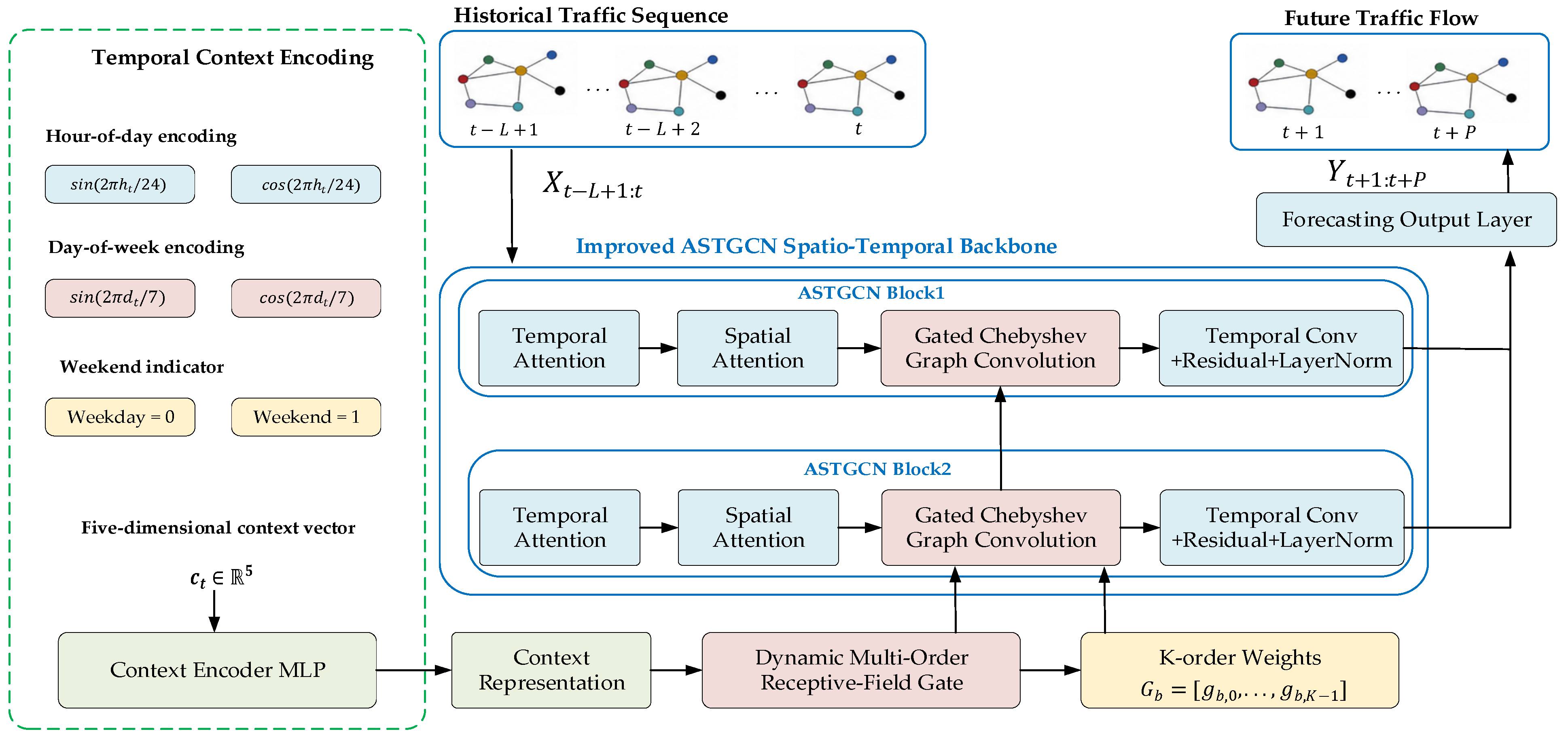
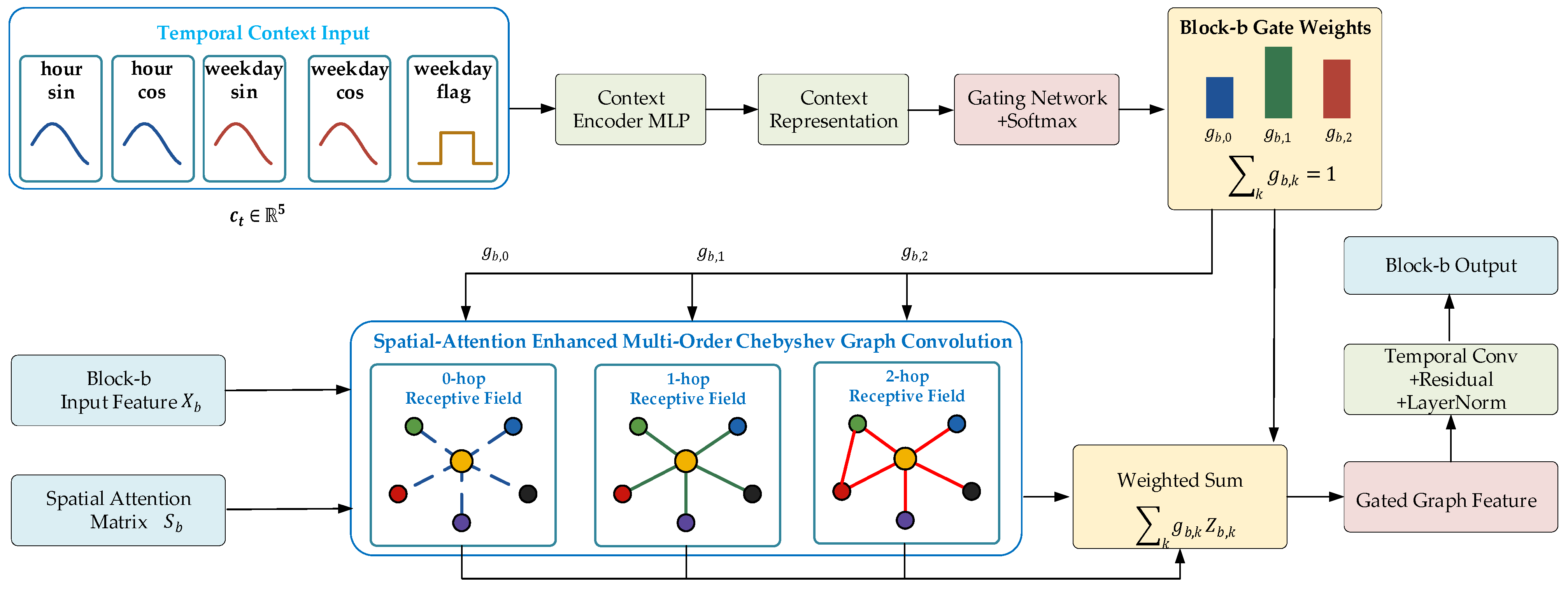
CD-MRFG addresses this narrow limitation while retaining the ASTGCN backbone. Its first contribution is a five-dimensional calendar-context encoding that separates periodic semantics from raw flow measurements. Its second contribution is a block-specific Softmax gate that converts the encoded context into weights for different Chebyshev orders. Its third contribution is an evaluation on PEMS03, PEMS04 and PEMS08 that combines reproduced baselines, module ablation, three-seed tests, gate diagnostics, complexity profiling, hyperparameter sensitivity and quantitative convergence analysis. The resulting claim is deliberately bounded: the method improves its direct ASTGCN baseline and exposes context-dependent order allocation, but it does not outperform every recent model.

The remainder of this paper is organized as follows. Section 2 reviews temporal, graph-based and context-aware forecasting methods and distinguishes CD-MRFG from related adaptive models. Section 3 defines the forecasting task and notation. Section 4 presents the model architecture and training objective. Section 5 reports the comparative, robustness, ablation, interpretation, efficiency, sensitivity and convergence results. Section 6 summarizes the findings and their limitations.

2. Related Work

2.1. Temporal and Statistical Traffic Forecasting

Classical approaches such as historical averages and autoregressive models are transparent but rely on stationary or linear assumptions. LSTM [1] and GRU [2] relax these assumptions through gated state transitions and capture nonlinear temporal dependence. Their main limitation for network forecasting is structural: each sensor is primarily treated as part of a sequence, so road-network propagation must be inferred indirectly.

2.2. Graph-Based Spatio-Temporal Forecasting

Graph neural networks represent sensors as nodes connected by physical or learned relations. STGCN combines graph and temporal convolutions [4], DCRNN models directed diffusion with recurrent graph operators [5], and Graph WaveNet learns an adaptive adjacency matrix with dilated temporal convolutions [6]. ASTGCN adds spatial and temporal attention to Chebyshev graph convolution [3]. AGCRN learns node-adaptive parameters and a data-adaptive graph [7], STSGCN constructs localized synchronous spatio-temporal graphs [13], and MTGNN jointly learns a directed graph, mix-hop propagation and multi-scale temporal filters [8]. These models adapt topology, node parameters or propagation operators, but they do not directly condition each Chebyshev order on calendar context. Other graph-based extensions include optimized temporal–spatial gated graph convolution [14], T-GCN [15], and spatial–temporal position-aware graph convolution [16]. MRA-BGCN is particularly relevant because it uses multi-range attention to learn the importance of different neighbourhood ranges from node- and edge-interaction features [17]. Unlike MRA-BGCN, CD-MRFG retains the ASTGCN backbone and conditions Chebyshev-order weights explicitly on an external calendar-context vector.

2.3. Context-Aware and Adaptive Traffic Modelling

Context-aware and attention-based methods model variation beyond fixed local graph convolution. GMAN links historical and future representations through spatio-temporal and transform attention [10]. STID uses spatial and temporal identity embeddings without explicit message passing [18]. MSGFormer combines multi-scale temporal modelling with gated Transformer components [9], while PDFormer introduces dynamic short- and long-range attention masks and propagation-delay-aware transformation [11]. STAEformer shows that adaptive spatio-temporal embeddings can make a vanilla Transformer highly competitive [12]. These approaches motivate context-dependent modelling, but their internal adaptive objects differ from the order-wise receptive-field allocation studied here. Traffic Transformer [19], ST-ResNet [20], and STDN [21] further demonstrate how periodicity, residual spatio-temporal structure, and dynamically changing dependencies can be incorporated into traffic prediction.

2.4. Differences from Existing Methods

CD-MRFG does not replace adaptive graph learning or Transformer attention. It retains the predefined road graph and ASTGCN feature extractor, then conditions the contribution of self, first-order and higher-order Chebyshev components on a five-dimensional calendar vector.

Table 1. Methodological differences between CD-MRFG and representative adaptive traffic forecasting models.

Model	Primary Adaptive Object	Graph Representation	Context or Scale Mechanism	Difference from CD-MRFG
ASTGCN [3]	Spatial and temporal attention	Predefined road graph	Static combination of Chebyshev orders	Direct backbone; no explicit calendar-conditioned order gate
Graph WaveNet [6]	Adaptive adjacency	Learned and predefined graphs	Dilated temporal convolution	Learns graph relations rather than calendar-conditioned order weights
AGCRN [7]	Node embeddings and node-specific parameters	Data-adaptive graph	Adaptive recurrent graph convolution	Adapts nodes and topology rather than explicit Chebyshev orders
GMAN [10]	Spatio-temporal attention	Attention-derived dependencies	Transform attention between historical and future states	Uses global attention instead of order-wise graph convolution
STID [18]	Spatial and temporal identities	No explicit graph propagation	Identity embeddings	Strong embedding baseline without an interpretable graph-order gate
MTGNN [8]	Directed graph and mix-hop propagation	Learned graph	Dilated inception temporal module	Learns topology and mix-hop features without calendar conditioning
Transformer models [9,11,12]	Attention, adaptive embeddings or delay masks	Global or dynamically masked relations	Long-range attention and multi-scale temporal modelling	Broader architectures; no explicit ASTGCN Chebyshev-order allocation
CD-MRFG	Chebyshev-order contribution	Predefined road graph	Five-dimensional calendar context and Softmax order gate	Lightweight ASTGCN extension with inspectable order weights

makes this distinction explicit. The method is, therefore, closest to a controlled, interpretable modification of ASTGCN, whereas Graph WaveNet, AGCRN and MTGNN adapt graph relations, STID adapts identity embeddings, and recent Transformers adapt attention or latent spatio-temporal embeddings.

3. Problem Formulation

3.1. Traffic Network Graph

In the traffic forecasting task, the road network is represented as a weighted graph G = (V, E, A), where V is the set of sensor nodes, E denotes road connectivity and A is the adjacency matrix. PEMS03, PEMS04 and PEMS08 contain 358, 307 and 170 sensors, respectively, and all flow records are aggregated at 5 min intervals.

$$X_t={\left[x_t^1,\cdots ,x_t^N\right]}^T\in R^{N\times C}$$

(1)

Here, $X_t$ denotes the traffic state of all nodes at time step t, and C is the feature dimension. This study uses only traffic flow, so C = 1.

3.2. Multi-Step Traffic Forecasting Task

Given a sequence of L historical traffic-flow steps $X_{t-L+1:t}$, the graph G and the temporal context vector $c_t$, the forecasting model learns a nonlinear mapping f_Theta to predict the next P time steps. Here, $X_{t-L+1:t}$ belongs to $R^{L\times N\times C}$, the predicted sequence belongs to $R^{P\times N\times C}$, and both L and P are set to 12 in all experiments. Therefore, the model uses the previous 1 h to forecast the next 1 h.

$${\widehat{X}}_{t+1:t+P}=f_{\theta }\left(X_{t-L+1:t},G,c_t\right)$$

(2)

3.3. Temporal Context Features

Traffic flow exhibits strong periodicity. The same sensor may follow different patterns across hours, weekdays and weekends. To represent this temporal context explicitly, a five-dimensional context vector is constructed at the forecasting origin:

$$c_t={\left[s_h,q_h,s_d,q_d,I_{\mathit{weekend}}\right]}^T\in R^5$$

(3)

$$s_h=\mathrm{s}\mathrm{i}\mathrm{n}\left({\displaystyle \frac{2\pi h_t}{24}}\right), q_h=\mathrm{c}\mathrm{o}\mathrm{s}\left({\displaystyle \frac{2\pi h_t}{24}}\right)$$

(4)

$$s_d=\mathrm{s}\mathrm{i}\mathrm{n}\left({\displaystyle \frac{2\pi d_t}{7}}\right), q_d=\mathrm{c}\mathrm{o}\mathrm{s}\left({\displaystyle \frac{2\pi d_t}{7}}\right)$$

(5)

where $h_t$ denotes the hour-of-day index in one day, $d_t$ denotes the day-of-week index in one week, and $I_{weekend}$ is the weekend indicator. The sine and cosine terms are used because hour and weekday are periodic variables.

3.4. Receptive Fields in Graph Convolution

Chebyshev graph convolution approximates a spectral graph filter with K polynomial orders. The k-th order can be interpreted as aggregating information from the k-hop neighborhood. The Chebyshev bases are defined recursively in Equations (6) and (7), where $T_k\left(\tilde{L}\right)$ denotes the k-th Chebyshev polynomial and $\tilde{L}$ is the scaled graph Laplacian. Different orders, therefore, correspond to different spatial receptive fields, whose contributions need not be identical for short-term forecasting [22,23].

$$T_0\left(\tilde{L}\right)=I_N, T_1\left(\tilde{L}\right)=\tilde{L}$$

(6)

$$T_k\left(\tilde{L}\right)=2\tilde{L}{T}_{k-1}\left(\tilde{L}\right)-T_{k-2}\left(\tilde{L}\right), k\ge 2$$

(7)

3.5. Evaluation Metrics

To evaluate multi-step traffic forecasting performance, this study uses mean absolute error (MAE), root mean square error (RMSE) and mean absolute percentage error (MAPE). MAE measures the average absolute deviation between predicted and observed traffic flows and provides a direct indication of overall forecasting accuracy. RMSE assigns larger penalties to large deviations and is, therefore, more sensitive to abrupt prediction errors around peak changes or congestion transitions. MAPE measures relative prediction error and is useful for comparing errors across different flow scales. Because traffic-flow records may contain zero or near-zero values, MAPE is calculated only on the valid set Ω, where the ground-truth value is larger than a small threshold. The three metrics are defined as follows:

$$\mathrm{M}\mathrm{A}\mathrm{E}={\displaystyle \frac{1}{M}}{\displaystyle \sum _{i=1}^M}\left|y_i-{\hat{y}}_i\right|$$

(8)

$$\mathrm{R}\mathrm{M}\mathrm{S}\mathrm{E}=\sqrt{{\displaystyle \frac{1}{M}}{\displaystyle \sum _{\mathrm{i}=1}^{\mathrm{M}}}{\left(y_i-{\hat{y}}_i\right)}^2}$$

(9)

$$\mathrm{M}\mathrm{A}\mathrm{P}\mathrm{E}={\displaystyle \frac{1}{\left|\Omega \right|}}\sum _{i\in \Omega }\left|{\displaystyle \frac{y_i-{\hat{y}}_i}{y_i}}\right|\times 100\%$$

(10)

For all three metrics, lower values indicate better forecasting performance. MAPE is reported as a decimal fraction throughout the paper.

4. CD-MRFG: Context-Driven Dynamic Gating for ASTGCN

As shown in Figure 1, CD-MRFG consists of an ASTGCN spatio-temporal backbone, a context feature embedding module, a dynamic multi-order receptive-field gating module and a forecasting head. Historical traffic flow is processed by temporal attention, spatial attention, Chebyshev graph convolution and temporal convolution. The temporal-context branch explicitly displays the cyclic hour-of-day and day-of-week encodings rather than empirical traffic-flow profiles. The weekend indicator is represented as a binary variable, with zero for weekdays and one for weekend days. The resulting context representation generates sample-dependent Chebyshev-order weights for each ASTGCN block, allowing the model to adjust the spatial propagation range according to the temporal operating condition.

4.1. ASTGCN Spatio-Temporal Backbone

The ASTGCN backbone contains temporal attention, spatial attention, Chebyshev graph convolution, temporal convolution and residual connections [1]. Temporal attention selects informative historical steps, whereas spatial attention produces a block-specific matrix $S_b$. Equation (11) gives the standard Chebyshev convolution. In CD-MRFG, the normalized spatial attention matrix is denoted by $\widehat{S_b}$, the order-specific propagation operator by $M_{b,k}$, and the corresponding feature by $Z_{b,k}$, as defined in Equations (14)–(16).

$$\mathrm{C}\mathrm{h}\mathrm{e}\mathrm{b}\mathrm{C}\mathrm{o}\mathrm{n}\mathrm{v}\left(\mathrm{X}\right)={\displaystyle \sum _{k=0}^{K-1}}{T}_k\left(\tilde{L}\right)\mathrm{X}{\mathsf{\Theta }}_k$$

(11)

4.2. Context Feature Embedding

The context embedding module maps $c_t$ to a sample-level hidden vector ${\mathrm{h}}_{\mathrm{c}}$ through a multilayer perceptron. This representation does not replace the traffic-flow input; instead, it provides conditional information for the gating network and captures differences in traffic propagation patterns under different temporal contexts.

$$h_c=\phi \left(c_t\right)=\mathrm{M}\mathrm{L}\mathrm{P}\left(c_t\right)$$

(12)

4.3. Dynamic Multi-Order Receptive-Field Gating

For the b-th ASTGCN block, the gating network generates a K-dimensional weight vector $g_b$ from $h_c$. After softmax normalization, the weights sum to one, allowing the model to select an appropriate spatial receptive field for each temporal context.

The motivation of the proposed gating mechanism is that different temporal contexts may require different spatial receptive fields. During peak hours, congestion may propagate to upstream and downstream sensors, so higher-order neighbourhoods may provide useful information. During off-peak periods, traffic states may be more locally stable, so lower-order neighbourhoods or self-information can be more reliable. Fixed Chebyshev-order weighting, therefore, restricts the modelling flexibility of graph convolution. By conditioning the order weights on temporal context, CD-MRFG provides a simple mechanism for representing context-dependent propagation ranges in a traffic network.

$$g_b=\mathrm{S}\mathrm{o}\mathrm{f}\mathrm{t}\mathrm{m}\mathrm{a}\mathrm{x}\left(W_g{h}_c+b_g\right),{\displaystyle \sum _{k=0}^{K-1 }}{g}_{b,k}=1$$

(13)

$$M_{b,k}=\left(T_k(\tilde{L})\odot \widehat{S_b}\right)$$

(14)

$$Z_{b,k}=M_{b,k}^{\mathrm{T}}{X}_b{\Theta }_{b,k}$$

(15)

$${\mathrm{Z}}_b={\displaystyle \sum _{k=0}^{K-1}}{g}_{b,k}{\mathrm{Z}}_{b,k}$$

(16)

Figure 2 details this modelling mechanism. The five-dimensional temporal context vector is first encoded as a hidden representation. The gate then produces sample-dependent K-order weights for the b-th ASTGCN block. Each Chebyshev order corresponds to self-information, local neighbourhood propagation or more distant neighbourhood propagation. The weighted sum forms a gated graph-convolution output, which is combined with temporal convolution, residual connection and layer normalization to update spatio-temporal features.

Algorithm 1 summarizes the dynamic gated graph convolution in the b-th ASTGCN block. The procedure keeps the original spatial-attention graph-convolution framework but adds a context-conditioned modelling layer that controls how different Chebyshev basis functions contribute to the simulated traffic propagation process.

Algorithm 1. Context-conditioned dynamic multi-order receptive-field gating
Input: traffic-flow feature Xb, temporal context vector ct, Chebyshev polynomial set $\left\{T_k\right(\tilde{L}\left)\right\},$ and spatial attention matrix Sb
Output: gated graph-convolution feature Zb of the b-th ASTGCN block
1.	hc ← MLPc(ct)
2.	Ab ← MLPg,b(hc)
3.	gb ← Softmax(Ab)
4.	$g_b=[g_{b,0},g_{b,1},\dots ,g_{b,K-1}],{\displaystyle \sum _{k=0}^{K-1}}{g}_{b,k}=1$
5.	Normalize Sb to obtain $\widehat{S_b}$
6.	Initialize Zb ← 0
7.	for k = 0, 1, …, K − 1 do
8.	if k = 0 then
9.	Mb,k ← I
10.	else
11.	$M_{b,k}\leftarrow \left(T_k(\tilde{L})\odot \widehat{S_b}\right)$
12.	end if
13.	Ub,k ← GraphConv(Xb, Mb,k, Θb,k)
14.	Zb ← Zb + gb,k Ub,k
15.	end for
16.	Zb ← ReLU(Zb + βb)
17.	return Zb

4.4. Training Objective

After the forecasting head produces the predicted sequence, CD-MRFG is optimized by minimizing the mean squared error between the predicted and observed traffic flows. Let $y_i$ and ${\widehat{y}}_i$ denote the ground-truth and predicted values over all valid nodes, horizons and samples. The residual term and training loss are defined in Equations (17) and (18).

$$e_i=y_i-{\widehat{y}}_i$$

(17)

$$L={\displaystyle \frac{1}{M}}{\displaystyle \sum _{i=1}^M}{e_i}^2$$

(18)

5. Experiments and Results

Experiments were conducted on PEMS03, PEMS04 and PEMS08. The evaluation addressed six questions: whether CD-MRFG improves its direct ASTGCN baseline, whether the result generalizes to a third sensor network, how it compares with recent strong baselines, whether the gains persist across random seeds, which components and hyperparameters control performance, and whether the added mechanism has acceptable computational and optimization costs. Unless otherwise stated, all reproduced models used the same chronological split, 12-step input, 12-step target and test metrics.

5.1. Datasets

PEMS03, PEMS04 and PEMS08 are public California freeway detector datasets sampled every 5 min. As shown in

Table 2. Dataset statistics.

Dataset	Nodes	Time Steps	Time Range
PEMS03	358	26,208	1 September 2018 to 30 November 2018
PEMS04	307	16,992	1 January 2018 to 28 February 2018
PEMS08	170	17,856	1 July 2016 to 31 August 2016

, PEMS03 contains 358 sensors and 26,208 time steps from 1 September to 30 November 2018. PEMS04 contains 307 sensors and 16,992 time steps from 1 January to 28 February 2018, and PEMS08 contains 170 sensors and 17,856 time steps from 1 July to 31 August 2016. Each dataset was divided chronologically into training, validation and test sets using a 6:2:2 ratio. Twelve historical observations were used to forecast the following twelve observations.

5.2. Experimental Settings and Metrics

Experiments were run on a workstation with a 13th Gen Intel Core i7-13700K CPU and an NVIDIA GeForce RTX 4090D GPU. Architecture-specific objectives and validation-selected settings followed the corresponding implementations, while the data split, input length, forecast horizon and evaluation code were fixed. As shown in

Table 3. Experimental settings.

Dataset	Learning Rate	Batch Size	Optimizer	Input Steps	Forecast Steps	Graph Order	ST Blocks	Context Hidden Dimension
PEMS03	0.001	32	Adam	12	12	3	2	64
PEMS04	0.001	32	Adam	12	12	3	2	64
PEMS08	0.001	32	Adam	12	12	3	2	64

, ASTGCN and CD-MRFG used Adam, mean squared error, a learning rate of 0.001 and a batch size of 32. Their common configuration contained two spatio-temporal blocks, Chebyshev order K = 3, 64 graph and temporal filters, and a CD-MRFG context hidden dimension of 64. The controlled benchmark runs of CD-MRFG achieved an overall MAE and RMSE of 16.98 and 28.59 on PEMS03, 20.82 and 32.77 on PEMS04, and 17.24 and 26.84 on PEMS08. Repeated-seed statistics are reported separately in Section 5.4.

Following common practice in traffic forecasting, mean absolute error (MAE), root mean square error (RMSE) and masked mean absolute percentage error (MAPE) are used as metrics. Their formal definitions are given in Equations (8)–(10). Let Y and Ŷ denote the ground-truth and predicted traffic flows, N the number of sensors and T the prediction horizon. Because traffic flow may contain zero or near-zero values, MAPE is calculated only on the valid set Ω, where the ground-truth value is larger than ε. In this paper, ε is set to 1 × 10⁻⁵. A lower MAE and RMSE indicate smaller forecasting error. RMSE is more sensitive to large errors, whereas MAPE measures relative error.

5.3. Comparison with Baseline Methods

The comparison includes HA, LSTM, GRU, DCRNN, STGCN, ASTGCN, AGCRN and STSGCN. All values in

Table 4. Forecasting performance of CD-MRFG and reproduced baselines on PEMS03, PEMS04 and PEMS08 datasets.

Dataset	Model	5 min		15 min		30 min		45 min		60 min		Average
		MAE	RMSE	MAE	RMSE	MAE	RMSE	MAE	RMSE	MAE	RMSE	MAE	RMSE
PEMS03	HA	26.17	47.51	26.17	47.50	26.16	47.50	26.16	47.50	26.15	47.49	26.16	47.50
	LSTM	13.39	22.98	16.11	27.39	19.32	31.95	22.65	36.63	26.23	41.50	19.88	33.12
	GRU	13.41	23.12	16.12	27.48	19.35	32.28	22.67	36.89	26.30	41.85	19.91	33.37
	DCRNN	12.74	20.31	15.26	24.59	17.70	28.45	20.12	32.01	22.55	35.50	18.00	29.08
	STGCN	16.61	27.05	18.11	29.40	19.76	31.91	21.53	34.49	23.58	37.48	20.09	32.49
	ASTGCN	13.47	22.78	15.85	26.60	18.27	30.30	20.76	33.88	23.55	37.70	18.66	31.05
	AGCRN	13.15	23.09	14.40	25.33	15.61	27.29	16.37	28.61	17.17	29.60	15.51	27.17
	STSGCN	14.20	23.18	15.91	26.12	17.54	28.83	19.12	31.46	20.89	34.23	17.75	29.31
	CD-MRFG	13.29	22.32	15.27	25.65	16.88	28.35	18.35	30.66	19.99	33.12	16.98	28.59
PEMS04	HA	26.04	41.66	26.04	41.66	26.05	41.67	26.06	41.67	26.06	41.67	26.05	41.67
	LSTM	18.33	28.97	21.22	33.12	24.89	38.29	28.86	43.62	33.17	49.40	25.66	39.71
	GRU	18.19	28.87	21.15	33.08	24.91	38.33	28.88	43.73	33.22	49.51	25.65	39.75
	DCRNN	17.40	27.59	19.88	30.96	22.06	33.94	24.07	36.57	25.93	39.07	22.18	34.23
	STGCN	22.49	35.59	23.88	37.36	25.71	39.70	28.03	42.64	30.89	46.28	26.33	40.62
	ASTGCN	18.30	28.78	20.34	31.62	22.38	34.40	24.57	37.21	27.23	40.62	22.79	35.02
	AGCRN	17.86	28.63	18.59	29.98	19.56	31.66	20.07	32.46	20.63	33.33	19.44	31.44
	STSGCN	17.96	28.49	19.54	30.93	21.21	33.55	22.84	35.86	24.45	38.10	21.38	33.81
	CD-MRFG	17.52	27.94	19.19	30.39	20.65	32.51	22.01	34.39	23.77	36.70	20.82	32.77
PEMS08	HA	23.27	40.56	23.26	40.55	23.25	40.52	23.23	40.50	23.22	40.47	23.24	40.52
	LSTM	13.92	21.38	16.49	25.64	19.54	30.56	22.68	35.00	26.32	39.96	20.10	31.56
	GRU	13.94	21.43	16.54	25.74	19.68	30.75	22.90	35.34	26.50	40.15	20.23	31.75
	DCRNN	13.35	20.35	15.65	23.96	17.23	26.52	18.85	28.75	20.20	30.68	17.33	26.68
	STGCN	20.06	30.32	20.98	31.66	22.26	33.59	23.81	35.71	25.85	38.47	22.68	34.18
	ASTGCN	15.35	23.28	17.12	26.19	19.11	29.18	21.03	31.91	23.47	35.22	18.88	28.83
	AGCRN	13.77	21.24	14.73	23.15	15.74	25.10	16.61	26.68	17.35	27.81	15.77	25.17
	STSGCN	14.15	21.58	15.72	24.36	17.13	26.88	18.52	29.17	19.96	31.31	17.28	27.18
	CD-MRFG	13.94	21.43	15.75	24.48	17.15	26.74	18.36	28.46	20.04	30.72	17.24	26.84

were reproduced with the common chronological split and evaluation code. Model-specific architecture and optimization settings followed their implementations and were selected using validation data. ASTGCN is the primary controlled baseline because CD-MRFG modifies its graph-convolution stage. STID and MTGNN are reported separately in

Table 5. Three-seed robustness and paired significance tests for ASTGCN and CD-MRFG.

Dataset	Model	MAE	RMSE	MAPE
PEMS04	ASTGCN	22.2984 ± 0.4829	34.5454 ± 0.6468	0.1563 ± 0.0054
PEMS04	CD-MRFG	21.7245 ± 0.3839	33.9865 ± 0.5087	0.1563 ± 0.0104
PEMS08	ASTGCN	18.8479 ± 0.7684	28.7259 ± 1.0694	0.1232 ± 0.0089
PEMS08	CD-MRFG	16.8782 ± 0.0561	26.2775 ± 0.1286	0.1151 ± 0.0020

as recent strong baselines on PEMS04 and PEMS08.

Errors increased with the prediction horizon for the learned baselines on all three datasets. On PEMS03, CD-MRFG achieved an overall MAE and RMSE of 16.98 and 28.59. It improved DCRNN by 5.67% in MAE and 1.68% in RMSE, STGCN by 15.48% and 12.00%, and STSGCN by 4.34% and 2.46%, respectively. AGCRN remained more accurate, with an overall MAE and RMSE of 15.51 and 27.17. The third dataset, therefore, supports generalization beyond PEMS04 and PEMS08 while preserving the bounded accuracy claim.

On PEMS04, CD-MRFG reduced overall MAE and RMSE by 6.13% and 4.25% relative to DCRNN, and by 20.93% and 19.32% relative to STGCN. On PEMS08, it reduced MAE by 0.52% relative to DCRNN, whereas its RMSE was 0.60% higher. AGCRN produced lower overall errors than CD-MRFG on PEMS04 and PEMS08. These mixed results show that the proposed gate improves an ASTGCN-style model but does not dominate adaptive graph learning.

The direct ASTGCN comparison was consistent across datasets. CD-MRFG reduced overall MAE and RMSE from 18.66 and 31.05 to 16.98 and 28.59 on PEMS03, from 22.79 and 35.02 to 20.82 and 32.77 on PEMS04, and from 18.88 and 28.83 to 17.24 and 26.84 on PEMS08. The corresponding MAE reductions were 9.00%, 8.64% and 8.69%. This controlled comparison supports the specific claim that explicit calendar context and order gating improve the ASTGCN backbone.

Table 6. Overall comparison with reproduced recent strong baselines on PEMS04 and PEMS08.

Dataset	Model	Role	Best Epoch	MAE	RMSE	MAPE
PEMS04	CD-MRFG	Context-gated ASTGCN extension	23	20.82	32.77	0.14
	STID [18]	Identity-embedding baseline	86	18.40	29.92	0.13
	MTGNN [8]	Adaptive graph and mix-hop baseline	100	19.05	31.62	0.13
PEMS08	CD-MRFG	Context-gated ASTGCN extension	59	17.24	26.84	0.11
	STID [18]	Identity-embedding baseline	89	14.22	23.40	0.09
	MTGNN [8]	Adaptive graph and mix-hop baseline	98	15.47	24.52	0.10

provides a stricter comparison with STID and MTGNN. Both recent baselines achieved lower overall errors than CD-MRFG on PEMS04 and PEMS08. The proposed method is, therefore, evaluated for its controlled gain over ASTGCN, explicit order-level diagnostics and modest architectural change, not for state-of-the-art accuracy.

MTGNN and STID benefit from learned graph structure or strong identity embeddings and, therefore, define an important accuracy boundary. Their advantage does not invalidate the controlled ASTGCN comparison, but it prevents a universal superiority claim.

5.4. Robustness Across Random Seeds

ASTGCN and CD-MRFG were independently trained with seeds 1, 42 and 2026 on PEMS04 and PEMS08. Table 5 reports mean ± standard deviation over the three runs. Paired two-sided t-tests compare the two models using matched seeds. Given the small sample size, the p-values are interpreted together with the paired differences rather than as standalone proof.

CD-MRFG reduced the mean MAE for every matched seed. The MAE difference was significant on PEMS04 (p = 0.028) and PEMS08 (p = 0.042). The mean RMSE was also lower, but the paired tests did not cross the 0.05 threshold on PEMS04 (p = 0.181) or PEMS08 (p = 0.057). MAPE differences were not significant. These results support a reproducible MAE gain while placing an explicit statistical boundary on the RMSE and MAPE claims.

5.5. Ablation Study

Four variants are evaluated on PEMS04 and PEMS08 to isolate the effect of each component. M1 is the original ASTGCN baseline. M2 adds fixed multi-order graph-convolution gating to ASTGCN. M3 uses only the context feature embedding module. M4, namely CD-MRFG, combines context embedding with dynamic multi-order receptive-field gating.

Table 7. Average 12-step results of the ablation variants on PEMS04 and PEMS08.

Model	PEMS04			PEMS08
	MAE	RMSE	MAPE	MAE	RMSE	MAPE
M1 ASTGCN	22.79	35.02	0.15	18.88	28.83	0.12
M2 fixed multi-order gating	22.78	36.45	0.15	18.85	28.56	0.13
M3 context embedding	21.34	33.81	0.14	17.83	27.25	0.11
M4 CD-MRFG	20.82	32.77	0.14	17.24	26.84	0.11

reports the average 12-step results.

• M1 ASTGCN. This baseline measures the forecasting ability of the original spatio-temporal attention graph convolution without temporal context or multi-order gating. Its average MAE is 22.79 and RMSE is 35.02 on PEMS04, while its average MAE is 18.88 and RMSE is 28.83 on PEMS08. These results show that ASTGCN captures basic spatio-temporal dependencies, but its input remains dominated by historical flow values and does not explicitly encode temporal context.
• M2 fixed multi-order graph-convolution gating. M2 does not provide a neutral modification to the ASTGCN baseline. On PEMS04, its MAE remains nearly unchanged, decreasing from 22.79 to 22.78, whereas its RMSE increases from 35.02 to 36.45, corresponding to a relative deterioration of 4.08%. Because RMSE assigns greater weight to large residuals, this divergence indicates that fixed order weighting increases the magnitude of difficult forecasting errors even when the average absolute error remains stable. A fixed gate applies the same receptive-field mixture to all samples and cannot distinguish traffic states dominated by local variation from states involving broader spatial propagation. This mismatch can cause excessive neighbourhood aggregation in local regimes or insufficient higher-order propagation during spatially extended congestion. On PEMS08, M2 produces only marginal reductions in MAE and RMSE, from 18.88 and 28.83 to 18.85 and 28.56, respectively, while MAPE increases from 0.12 to 0.13. The opposite RMSE changes across datasets indicate that a fixed receptive-field mixture interacts with dataset-specific topology and traffic-regime composition rather than providing a robust improvement. In contrast, M4 conditions the order weights on temporal context and reduces the PEMS04 RMSE from 36.45 to 32.77 and the PEMS08 RMSE from 28.56 to 26.84 relative to M2. These results indicate that the effectiveness of multi-order gating depends on sample-specific contextual modulation rather than on the introduction of additional order weights alone.
• M3 context feature embedding. This variant evaluates the contribution of temporal context itself. M3 reduces MAE to 21.34 and RMSE to 33.81 on PEMS04 and reduces MAE to 17.83 and RMSE to 27.25 on PEMS08, clearly outperforming M1 on both datasets. Hour, weekday and weekend indicators, therefore, provide useful periodic semantics that help distinguish morning and evening peaks, off-peak periods and weekend traffic.
• M4 CD-MRFG. The full model combines context embedding with dynamic multi-order receptive-field gating and achieves the best results among the four variants. It obtains an MAE of 20.82, RMSE of 32.77 and MAPE of 0.14 on PEMS04, and an MAE of 17.24 and RMSE of 26.84 on PEMS08. Its further improvement over M3 indicates that context is useful not only as an auxiliary input representation but also as a condition for selecting graph-convolution orders.

5.6. Gate Weight Analysis Under Different Traffic Periods

Gate weights were extracted from the PEMS04 and PEMS08 test sets to determine whether order allocation changed with temporal context.

Table 8. Mean dynamic gate weights under different traffic periods.

Dataset	Traffic Period	Samples	Block	Order 0	Order 1	Order 2
PEMS04	Morning peak	432	1	0.440	0.036	0.524
PEMS04	Morning peak	432	2	0.010	0.748	0.242
PEMS04	Daytime off-peak	1008	1	0.352	0.054	0.594
PEMS04	Daytime off-peak	1008	2	0.107	0.362	0.531
PEMS04	Evening peak	432	1	0.431	0.355	0.214
PEMS04	Evening peak	432	2	0.576	0.034	0.390
PEMS04	Night	1522	1	0.285	0.306	0.409
PEMS04	Night	1522	2	0.519	0.282	0.199
PEMS08	Morning peak	432	1	0.523	0.476	0.002
PEMS08	Morning peak	432	2	0.248	0.044	0.707
PEMS08	Daytime off-peak	1046	1	0.506	0.483	0.012
PEMS08	Daytime off-peak	1046	2	0.291	0.012	0.697
PEMS08	Evening peak	468	1	0.410	0.468	0.123
PEMS08	Evening peak	468	2	0.145	0.209	0.646
PEMS08	Night	1621	1	0.361	0.589	0.050
PEMS08	Night	1621	2	0.192	0.358	0.450

Note: Order 0 denotes self-information, order 1 denotes first-order neighbor propagation, and order 2 denotes second-order neighborhood propagation. Values are averaged over test samples in each traffic period.

reports the mean weights assigned to orders 0, 1 and 2 in the two ASTGCN blocks for four traffic periods. Each row sums to one because the gate uses a Softmax output.

The distributions varied across traffic periods and blocks. On PEMS04, block 1 emphasized order 2 during the morning peak and daytime off-peak periods, whereas block 2 emphasized order 1 in the morning peak and order 0 in the evening peak and at night. On PEMS08, block 1 mainly balanced orders 0 and 1, while block 2 assigned larger weights to order 2 in the three daytime periods. The gate, therefore, did not collapse to a single fixed mixture.

These weights are model-internal allocation coefficients, not measurements of physical traffic propagation or causal influence. Their variation supports the narrower conclusion that CD-MRFG uses different polynomial graph components under different calendar contexts. Physical interpretation would require external traffic-state evidence or controlled interventions.

5.7. Model Interpretation and Applicability Boundary

CD-MRFG is designed for short-term forecasting on fixed sensor graphs with regular daily and weekly regimes. The gate converts calendar context into a convex combination of self, first-order and higher-order graph features. This construction makes the model’s receptive-field preference inspectable without replacing the ASTGCN backbone.

The applicability boundary is equally important. The five context variables do not represent holidays, incidents, weather, roadworks or special events. The method may, therefore, be less reliable when non-recurring disturbances dominate the traffic state. It also retains a predefined graph and cannot recover missing or evolving connectivity as directly as adaptive graph-learning models.

AGCRN, STID and MTGNN achieved lower absolute errors in several comparisons. CD-MRFG should, thus, be used when the objective is a controlled ASTGCN improvement with explicit order-level diagnostics and modest structural change, rather than when forecasting accuracy alone determines model choice.

5.8. Complexity and Computational Overhead

Because CD-MRFG adds only a context encoder and a dynamic receptive-field gate to ASTGCN, its overhead mainly comes from lightweight multilayer perceptrons and scalar order-wise weighting.

Table 9. Parameter scale and computational profiling results.

Dataset	Model	Parameters (M)	Checkpoint Size (MB)	Latency (ms per Batch)	Throughput (Samples per Second)
PEMS04	ASTGCN	0.450031	1.7287	24.0594	1330.04
PEMS04	CD-MRFG	0.459125	1.7664	27.8637	1148.4482
PEMS08	ASTGCN	0.179456	0.6966	17.9400	1783.7233
PEMS08	CD-MRFG	0.188550	0.7342	19.5344	1638.1363

reports profiling under a batch size of 32 on CUDA. On PEMS04, the parameter count increases from 0.450 M to 0.459 M, and latency increases from 24.06 ms to 27.86 ms. On PEMS08, the parameter count increases from 0.179 M to 0.189 M, and latency increases from 17.94 ms to 19.53 ms. The measured PEMS08 checkpoint sizes are 0.6966 MB for ASTGCN and 0.7342 MB for CD-MRFG. The measured values indicate limited model-size growth and moderate inference overhead.

5.9. Hyperparameter Sensitivity

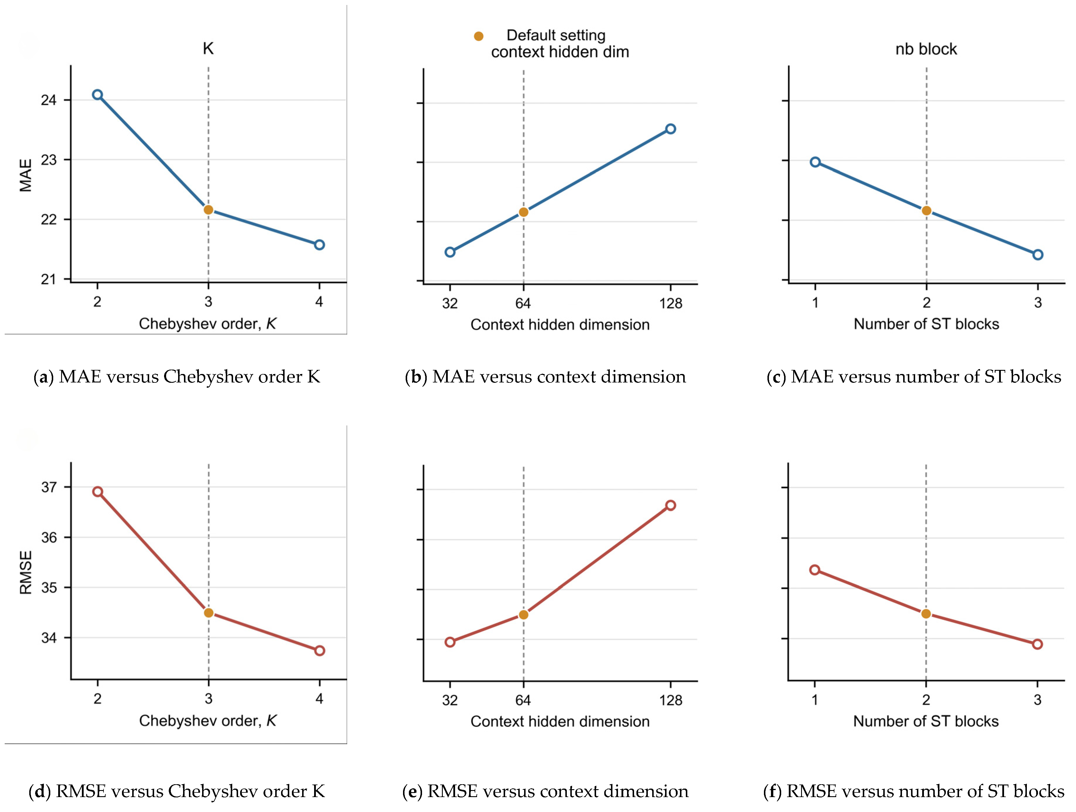
A one-factor-at-a-time analysis was conducted on PEMS04 with seed 42. Chebyshev order K, context hidden dimension and the number of spatio-temporal blocks were varied while the remaining settings were fixed. The analysis was performed after the main benchmark and was not used to retrospectively select the reported test configuration.

Table 10. PEMS04 hyperparameter sensitivity results.

Parameter	Value	MAE	RMSE	MAPE	Parameters	Training Time (min)
Chebyshev order K	2	24.0911	36.9084	0.1863	454 835	29.90
Chebyshev order K	3 (default)	22.1575	34.4952	0.1681	459 125	34.70
Chebyshev order K	4	21.5715	33.7388	0.1522	463 415	38.56
Context hidden dimension	32	21.4833	33.9454	0.1506	452 533	34.39
Context hidden dimension	64 (default)	22.1575	34.4952	0.1681	459 125	34.70
Context hidden dimension	128	23.5661	36.6847	0.1695	484 597	33.17
ST blocks	1	22.9722	35.3628	0.1745	220 353	17.83
ST blocks	2 (default)	22.1575	34.4952	0.1681	459 125	34.70
ST blocks	3	21.4221	33.8859	0.1405	697 897	52.15

reports PEMS04 hyperparameter sensitivity results and Figure 3 demonstrates PEMS04 sensitivity to the varied parameters.

Increasing K from 2 to 4 progressively reduced MAE and RMSE, but K = 4 increased training time by 11.1% relative to K = 3. A hidden dimension of 32 was more accurate and smaller than the default 64, whereas 128 degraded both errors, indicating that a larger context encoder is not automatically beneficial. Three blocks achieved the lowest errors but increased parameters and training time by about 52% and 50% relative to two blocks. The main setting, therefore, represents a fixed benchmark configuration rather than the best point from post hoc tuning.

5.10. Quantitative Convergence Analysis

Table 11. Quantitative convergence results over three random seeds.

Dataset	Model	E90	E95	Normalized AUC	Tail CV (%)	Optimization Time (min)
PEMS04	ASTGCN	4.33 ± 2.31	7.67 ± 3.06	0.0222 ± 0.0039	1.25 ± 0.42	31.13 ± 0.54
PEMS04	CD-MRFG	4.00 ± 1.00	8.00 ± 3.46	0.0190 ± 0.0025	1.21 ± 0.72	35.71 ± 2.55
PEMS08	ASTGCN	4.67 ± 2.08	7.33 ± 2.52	0.0262 ± 0.0026	3.18 ± 1.37	22.11 ± 0.10
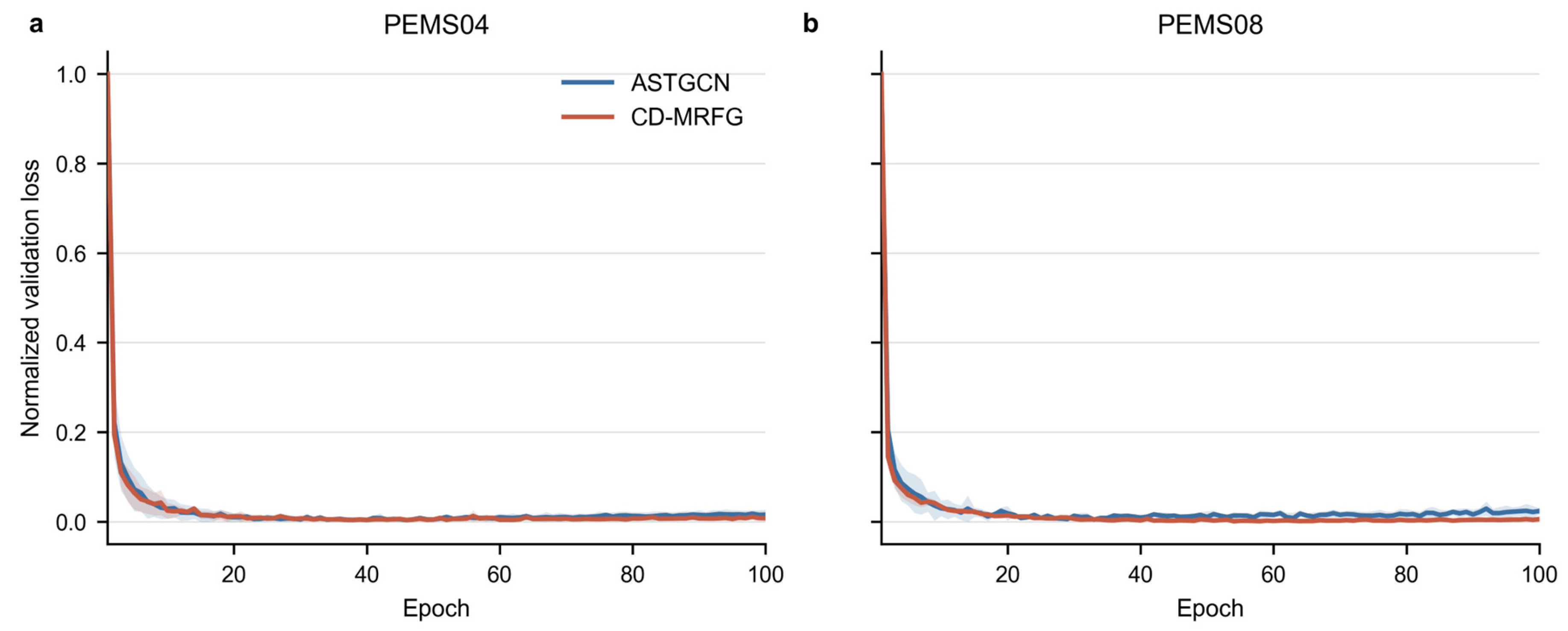
PEMS08	CD-MRFG	3.33 ± 0.58	7.00 ± 2.00	0.0163 ± 0.0011	0.84 ± 0.36	26.28 ± 0.47

reports quantitative convergence results from the completed three-seed logs. E90 and E95 denote the first epochs that reached 90% and 95% of the final achieved validation-loss reduction. In Figure 4, normalized area under the validation curve (AUC) summarizes the full optimization trajectory, with a smaller value indicating faster loss reduction. Late-stage variability is measured by the coefficient of variation over the final ten epochs.

Both models reached E90 within approximately five epochs. CD-MRFG had a lower normalized AUC on both datasets. The paired difference was significant on PEMS08 (p = 0.031) and marginal on PEMS04 (p = 0.054). On PEMS08, CD-MRFG also reduced late-stage variability from 3.18% to 0.84%. These optimization benefits required additional time: the mean training duration increased by 4.58 min on PEMS04 and 4.16 min on PEMS08. The results support a more efficient loss trajectory, particularly on PEMS08, rather than a universal claim of faster threshold attainment.

5.11. Forecasting Visualization

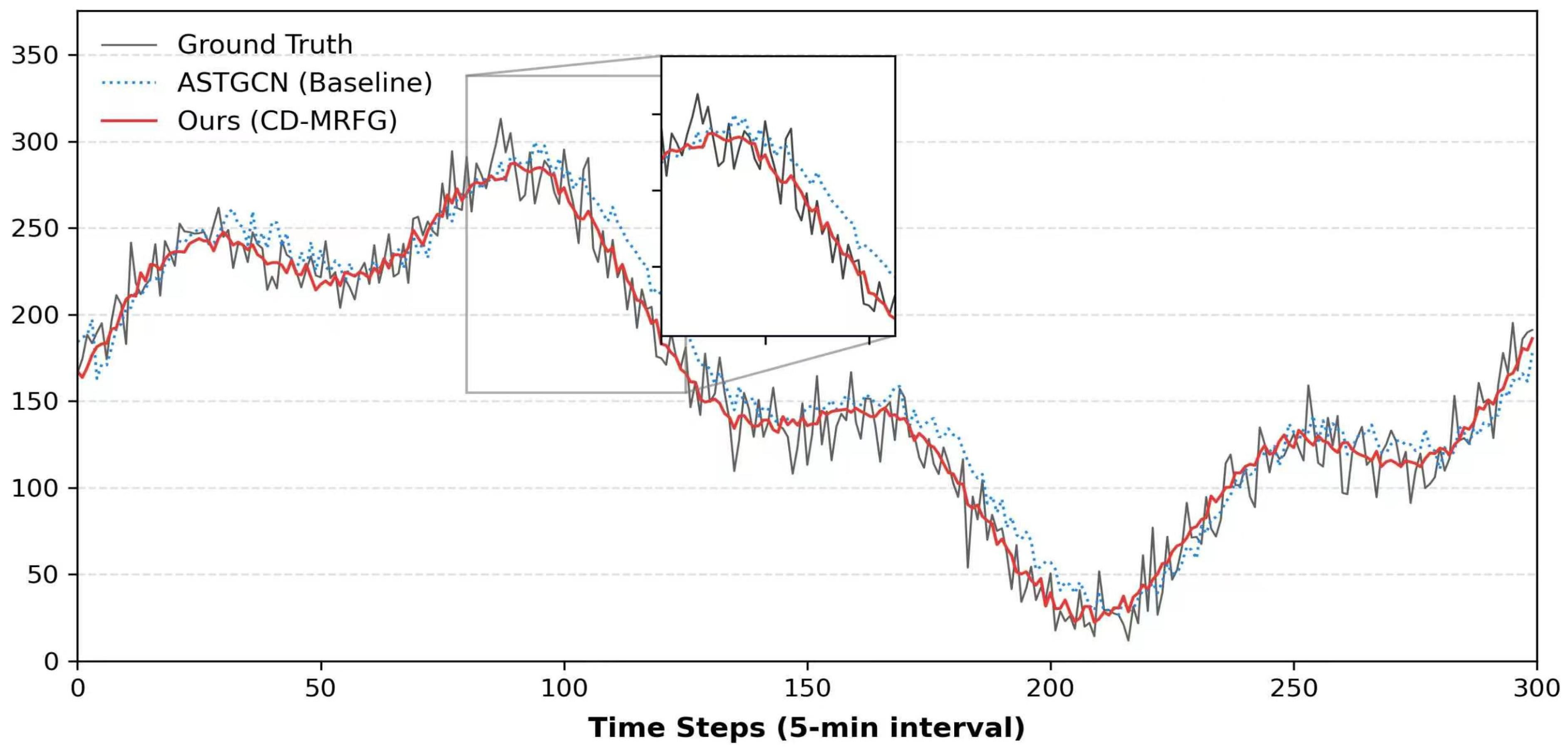
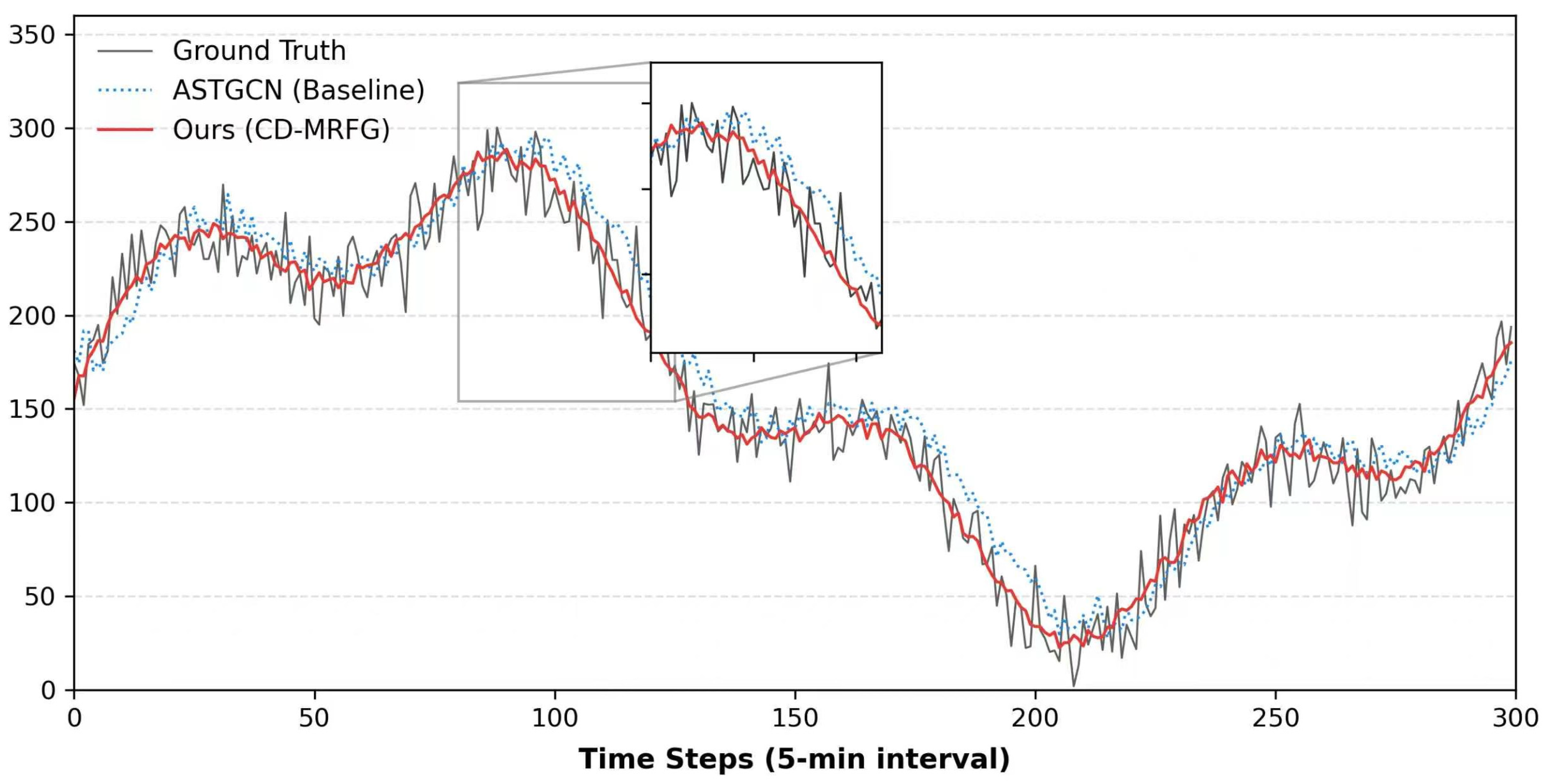
In Figure 5 and Figure 6, representative PEMS04 and PEMS08 test sequences are plotted with ground-truth flow, ASTGCN predictions and CD-MRFG predictions. The curves provide qualitative evidence about turning-point response and trend continuity. PEMS03 is evaluated quantitatively in Table 4 but is not used to select an additional visualization.

On PEMS04, the selected sequence contains evident morning-like growth, a high-flow plateau, subsequent decline and recovery. These stages are useful for evaluating multi-step forecasting because errors easily accumulate around turning points. The ASTGCN baseline captures the broad temporal trend, but its predicted curve tends to lag when the flow changes quickly. CD-MRFG gives a smoother yet more responsive trajectory, especially around the falling segment after the local peak and the later recovery interval.

The PEMS08 visualization provides a second case with a different sensor scale and temporal distribution. Although the overall profile differs from PEMS04, the same phenomenon can be observed: baseline predictions are delayed in several peak-decline and trough-recovery intervals, whereas CD-MRFG remains closer to the ground-truth direction of change. This cross-dataset consistency supports the argument that the proposed context-conditioned gate improves the dynamic selection of spatial receptive fields instead of overfitting one particular dataset.

The visual results complement the aggregate errors in Table 4. They show that CD-MRFG follows several rise, decline and recovery segments more closely than ASTGCN. These examples are illustrative rather than statistical evidence and should be interpreted together with the full test-set metrics and repeated-seed analysis.

6. Conclusions

This paper presented CD-MRFG, a context-gated ASTGCN extension that maps calendar information to Chebyshev-order weights. Controlled experiments on PEMS03, PEMS04 and PEMS08 consistently improved the direct ASTGCN baseline, and three-seed tests confirmed significant mean MAE reductions on PEMS04 and PEMS08. Ablation identified temporal context as the main contributor, while gate diagnostics showed non-constant order allocation across periods and blocks. Sensitivity and convergence analyses further exposed the effects of model scale and the associated optimization cost. CD-MRFG did not outperform AGCRN, STID or MTGNN in every setting, and its gate weights are not causal measurements of traffic propagation. The method is, therefore, most appropriate as a lightweight and inspectable improvement to ASTGCN on fixed sensor graphs with recurring calendar regimes.