Surrogate Modeling and Optimization of a Dual-Band Circular Patch Antenna with a C-Shaped Slot Using MLP Neural Networks

Abstract

This paper presents an efficient framework for surrogate modeling and rapid optimization of a dual-band circular patch antenna with a C-shaped slot (DB-CPAC) using multilayer perceptron (MLP) neural networks. Although highly accurate, traditional full-wave electromagnetic simulations are computationally expensive for geometric optimization due to complex slot-induced surface current perturbations. To address this limitation, a hybrid optimization framework based on Latin Hypercube Sampling (LHS) is proposed, combining the developed MLP model with a Method-of-Moments (MoM) simulator. The surrogate model uses an advanced modular architecture consisting of an ensemble of MLP neural networks for regressing center frequencies and classification MLP modules with a softmax output layer to estimate the probabilities of achieving bandwidth and gain targets. All networks are trained using the Levenberg–Marquardt algorithm with early stopping on data generated by a dedicated DB-CPAC_MoM_Sim software package. The proposed LHS-based optimizer employs the surrogate model for rapid global search and targeted local optimization before final MoM verification. Results show that this hybrid approach achieves an order-of-magnitude acceleration of the optimization process compared to conventional MoM methods while maintaining high accuracy.

1. Introduction

The rapid advancement of modern wireless communication systems, including 5G networks, satellite communications, and GPS applications, has imposed strict requirements on the design and optimization of microwave antennas. Microstrip patch antennas are widely used due to their low profile, cost-effectiveness, ease of integration with RF front-end, and multiband capabilities [1,2,3]. Among various geometric configurations, circular patch antennas are of particular interest for their specific radiation characteristics, polarization stability, and flexibility in achieving multiband operations [4,5,6,7].

One of the most effective methods for achieving dual-band behavior in circular microstrip antennas is the introduction of dedicated slots on the radiating element, among which the C-shaped slot is often used [8,9,10,11]. However, the introduction of slots significantly disrupts the regular surface current paths and distribution, as well as the overall resonant characteristics of the antenna. Because of this non-uniformity, standard analytical models and equivalent RLC circuits fail to accurately predict the antenna’s input impedance, making them impractical for modern design procedures [4]. Consequently, antenna designers primarily rely on numerical full-wave electromagnetic methods, such as the Method of Moments (MoM) or the Finite Element Method (FEM) [12,13,14]. Although these methods provide high accuracy, their iterative execution within multidimensional optimization loops requires significant computational resources and run-time, making the antenna optimization process slow and inefficient.

To overcome these computational challenges, surrogate modelling techniques based on artificial neural networks (ANNs) [15,16] have recently been successfully applied in electromagnetics [17,18]. Among various network architectures, multilayer perceptrons (MLPs) have proven to be powerful and reliable tools for approximating nonlinear mappings in the microwave domain [19,20,21,22,23,24,25,26]. Once trained, neural networks enable the creation of models capable of predicting key antenna characteristics in a fraction of a second. However, traditional approaches mostly rely on pure regression to directly predict resonant frequencies, which may be insufficient when the design must simultaneously meet the thresholds for operational bandwidth and gain levels [23,24,25,26]. A more robust approach requires advanced modular frameworks that combine regression ensembles with classification modules to accurately assess the probability of meeting predefined conditions, thereby enabling efficient and accurate antenna design.

The main goal of this work is to present a novel hybrid framework for surrogate modelling and rapid optimization of a dual-band circular patch antenna with a C-shaped slot (DB-CPAC) with a minimal number of computationally expensive full-wave electromagnetic simulations. The proposed approach integrates an advanced modular MLP antenna model and a hybrid optimizer based on Latin Hypercube Sampling (LHS), paired with a MoM simulator implemented in the MATLAB R2023b environment [27,28,29]. The primary novelty of the proposed framework lies in its specialized modular architecture and optimization-oriented design strategy. Instead of approximating the complete frequency response of the antenna, as is common in many surrogate modeling approaches, the proposed framework directly models the antenna performance parameters required during optimization. Specifically, it employs an ensemble of regression MLP networks for precise estimation of the dual-band center frequencies, alongside dedicated classification MLP modules with softmax output layers to estimate the probabilities of satisfying the predefined bandwidth and gain criteria. These probabilistic feasibility indicators are directly incorporated into the optimization fitness function, enabling rapid identification and ranking of feasible antenna geometries. Furthermore, the proposed surrogate model is trained over a relatively wide six-dimensional design space, allowing substantial variations in both the C-shaped slot geometry and the feed position. This modular organization not only enables efficient surrogate-assisted optimization and significantly accelerates global search and local parameter refinement, but also provides a scalable framework that can be extended to multiband antennas by incorporating additional regression and classification modules for the corresponding operating bands.

After the Introduction, the remainder of this paper is organized as follows. Section 2 details the physical geometry of the antenna, the defined parameters, and the theoretical foundation of its electromagnetic modeling using equivalent circuits and the MoM simulator. Section 3 describes the proposed surrogate modeling framework, the detailed architecture of the MLP modules, the network training and testing procedures, and the operational algorithm of the LHS-based optimizer. Section 4 presents and discusses numerical results, including the accuracy analysis of the neural networks and the optimization performance. Finally, Section 5 outlines the main conclusions and directions for future research.

2. Geometry and Electromagnetic Modeling of the Dual-Band Circular Patch Antenna with a C-Shaped Slot

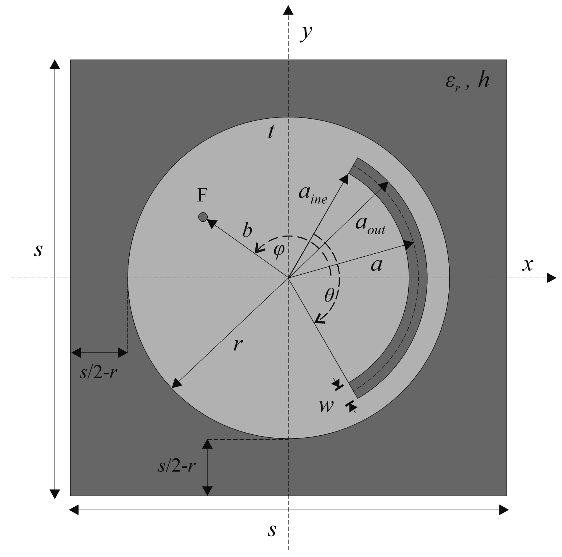
The physical geometry of the DB-CPAC is shown in Figure 1. The parameters defining its geometry and electromagnetic characteristics are as follows: s—substrate side length; h—substrate thickness; ε_r—relative dielectric permittivity of the substrate; t—metallization thickness; r—radius of the circular patch; θ—slot opening angle; a—distance of the slot centerline from the patch center (a_ine—distance of the inner slot edge from the patch center; a_out—distance of the outer slot edge from the patch center; a = (a_ine + a_out)/2); w—slot width (w = a_out − a_ine); b—distance of the feed point (F) from the patch center; and φ—angular position of the feed point relative to the patch x-axis, φ ∈ [0°, 360°].

In accordance with the analytical approach for modeling the electromagnetic characteristics of such antenna structures presented in [4], the proposed DB-CPAC can be considered as a resonant structure whose input impedance is given by the following:

$$z_{in}={\left({\displaystyle \frac{1}{z_{patch}}}+{\displaystyle \frac{1}{z_{slot}}}\right)}^{-1},$$

(1)

where z_patch represents the impedance of the circular patch resonator, and z_slot denotes the equivalent impedance introduced by the C-shaped slot. The patch resonator can be approximately represented by a parallel RLC circuit:

$$z_{patch}={\left({\displaystyle \frac{1}{R_p}}+{\displaystyle \frac{1}{j\omega L_p}}+j\omega C_p\right)}^{-1},$$

(2)

where R_p, L_p, and C_p denote the equivalent radiation resistance, inductance, and capacitance of the circular patch resonator, respectively. On the other hand, the slot can be modeled as an additional resonant element having the following:

$$z_{slot}=R_s+j\omega L_s+{\displaystyle \frac{1}{j\omega C_s}},$$

(3)

where R_s, L_s, and C_s represent the equivalent resistance, inductance, and capacitance associated with the C-shaped slot. The dual-band behavior of the proposed DB-CPAC can be clearly observed from Expressions (1) and (2).

For a resonant circular patch antenna without a slot operating in the dominant TM₁₁ mode, the input reactance at the resonance is approximately equal to zero, so that the input impedance becomes practically real. Therefore, for a circular patch of radius r fed at a distance b from the patch center, the following expression holds [4]:

$$z_{in}^{({\mathrm{TM}}_{11})}(r,b)\approx R_{edge}{\displaystyle \frac{J_1^2(k_{11}b)}{J_1^2(k_{11}{r}_e)}},$$

(4)

where R_edge is the resonant edge resistance of the circular patch antenna, which can be analytically determined using the expressions given in [4], J₁(⋅) is the Bessel function of the first kind, and k₁₁ denotes the resonant wave number associated with the dominant TM₁₁ mode, calculated as k₁₁ = 1.8412/r_e, where 1.8412 represents the first root of the derivative of the Bessel function J₁′(x), while r_e is the effective radius of the circular patch antenna calculated according to [4] as follows:

$$r_e=\sqrt{1+{\displaystyle \frac{2h}{\pi r{\epsilon }_r}}\left[\ln \left({\displaystyle \frac{\pi r}{2h}}\right)\right]+1.7726}.$$

(5)

However, the introduction of the C-shaped slot significantly perturbs the surface current distribution and produces strong electromagnetic coupling between the circular patch and the slot resonator. Consequently, although the equivalent circuit described by Equations (1)–(5) provides a conceptual physical interpretation of the dual-band operating mechanism, accurate extraction of the equivalent circuit parameters directly from the antenna geometry is not feasible. Therefore, the limitation lies not in the equivalent circuit itself, but in the absence of an analytical procedure capable of determining its parameters for the considered antenna geometry. For this reason, a full-wave electromagnetic model of the DB-CPAC antenna, based on the Method of Moments (MoM) and implemented using the MATLAB Antenna Toolbox [29], was employed to accurately characterize the antenna behavior and generate the training data for the proposed MLP-based surrogate model.

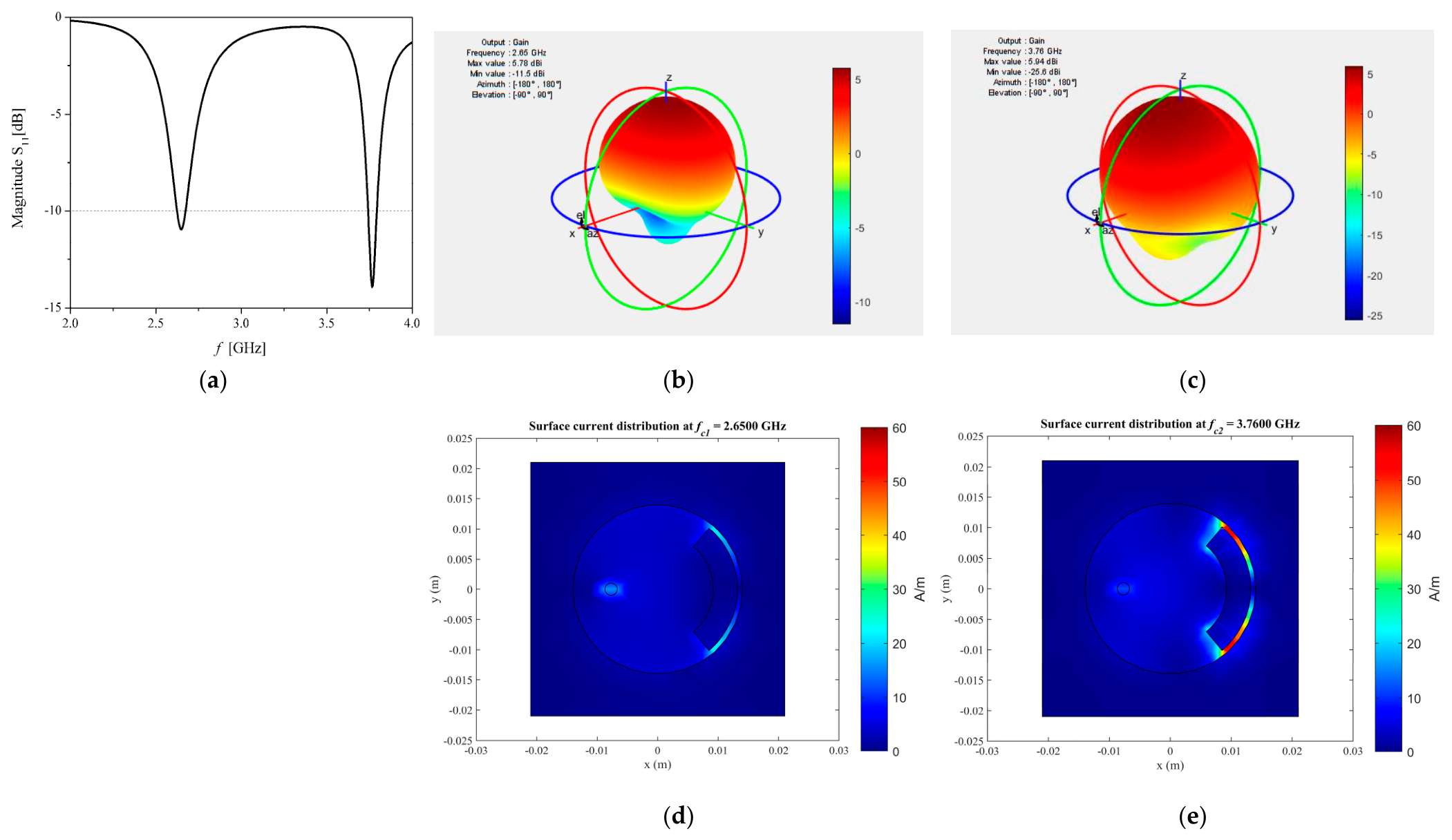
The aforementioned full-wave electromagnetic model of the DB-CPAC was integrated into the software package DB-CPAC_MoM_Sim, developed specifically for this study. Figure 2a, Figure 2b and Figure 2c show the simulated S₁₁ parameter versus frequency, the antenna radiation pattern at the center frequency of the first operating band, and the antenna radiation pattern at the center frequency of the second operating band, respectively, obtained using the DB-CPAC_MoM_Sim software package. The modeled DB-CPAC is realized on an FR4 substrate (ε_r = 4.8, tan δ = 0.026, h =1.6 mm) with the following physical parameter values: s = 7 mm, r = 14 mm, θ = 100°, a = 11.2 mm, w = 4 mm, b = 7.7 mm, and φ = 180°. During the simulations, the metallization thickness was neglected (t ≈ 0), while the metallic patch and ground plane were modeled as perfect electric conductors.

Figure 2d presents the surface current distribution of the proposed antenna at the center frequency of the first operating band (fc₁ = 2.65 GHz). It can be observed that the surface current is relatively uniformly distributed over the entire metallized patch, indicating that the lower-frequency resonance is associated with the oscillation mode governed primarily by the electromagnetic characteristics of the complete patch structure. In contrast, Figure 2e shows the surface current distribution at the center frequency of the second operating band (fc₂ = 3.70 GHz). A pronounced concentration of the surface current is observed in the vicinity of the C-shaped slot, indicating that the higher-frequency resonance is mainly governed by the electromagnetic characteristics of the slot. These current distributions provide additional physical insight into the operating principles responsible for the dual-band behavior of the proposed antenna.

3. MLP-Based Surrogate Modeling Framework for the DB-CPAC

The proposed DB-CPAC modeling framework consists of the following:

• An MLP-based DB-CPAC model for modeling the dependence of the key characteristics of the dual-band antenna on its physical parameters.
• An LHS ANN–MoM optimizer intended for fast surrogate-based optimization of the antenna physical parameters.

3.1. MLP-Based DB-CPAC Model

The MLP-based DB-CPAC model is designed to estimate the following antenna characteristics from the variable antenna physical parameters:

• Radius of the circular patch (r)
• Slot opening angle (θ)
• Distance of the slot centerline from the patch center (a)
• Slot width (w)
• Distance of the feed point (F) from the patch center (b)
• Angular position of the feed point relative to the patch x-axis (φ)

For fixed substrate parameters, the following is established:

• Substrate thickness (h)
• Relative dielectric permittivity of the substrate (ε_r)

The substrate side length is selected as s = 3r.

The outputs estimated by the proposed model are as follows:

• Center frequency of the first operating band (f_C1)
• Center frequency of the second operating band (f_C2)
• Satisfying Bandwidth Flag 1 (SBF₁)
• Estimated probability that SBF₁ = 1 (p_SBF1)
• Satisfying Bandwidth Flag 2 (SBF₂)
• Estimated probability that SBF₂ = 1 (p_SBF2)
• Satisfying Gain Flag 1 (SGF₁)
• Estimated probability that SGF₁ = 1 (p_SGF1)
• Satisfying Gain Flag 2 (SGF₂)
• Estimated probability that SGF₂ = 1 (p_SGF2)

The flag SBF₁ takes the value “1” if the normalized bandwidth of the first operating band is greater than or equal to the minimum acceptable bandwidth value FBW_1min; otherwise, it takes the value “0”. Similarly, SBF₂ indicates whether the normalized bandwidth of the second operating band satisfies the predefined bandwidth criterion FBW_2min.

Furthermore, SGF₁ takes the value “1” if the antenna gain at the center frequency of the first operating band is greater than or equal to the minimum acceptable gain value G_1min; otherwise, it takes the value “0”. Similarly, SGF₂ indicates whether the antenna gain at the center frequency of the second operating band satisfies the predefined gain criterion G_2min.

The estimated probabilities p_SBF1, p_SBF2, p_SGF1, and p_SGF2 are used for evaluation of the fitness function employed during the DB-CPAC optimization procedure.

Accordingly, the proposed MLP-based DB-CPAC model represents the nonlinear mapping:

$$\begin{array}{l}{[\begin{array}{cccccccccc}{f}_{C1}& f_{C2}& SB{F}_1& p_{\mathrm{SBF}1}& SB{F}_2& p_{\mathrm{SBF}2}& SG{F}_1& p_{\mathrm{SGF}1}& SG{F}_2& p_{\mathrm{SGF}2}\end{array}]}^{\mathrm{T}}=\\ {\mathsf{\Phi }}_{\mathrm{MLP}\_\mathrm{DB}-\mathrm{CPA}}\left({\left[\begin{array}{cccccc}r& \theta & a& w& b& \phi \end{array}\right]}^{\mathrm{T}}\right)={\mathsf{\Phi }}_{\mathrm{MLP}\_\mathrm{DB}-\mathrm{CPAC}}\left(x\right)\end{array},$$

(6)

where x = [r θ a w b φ]^T denotes the vector of the model input variables, while Φ(·) represents the nonlinear transfer function implemented by the proposed MLP-based DB-CPAC model.

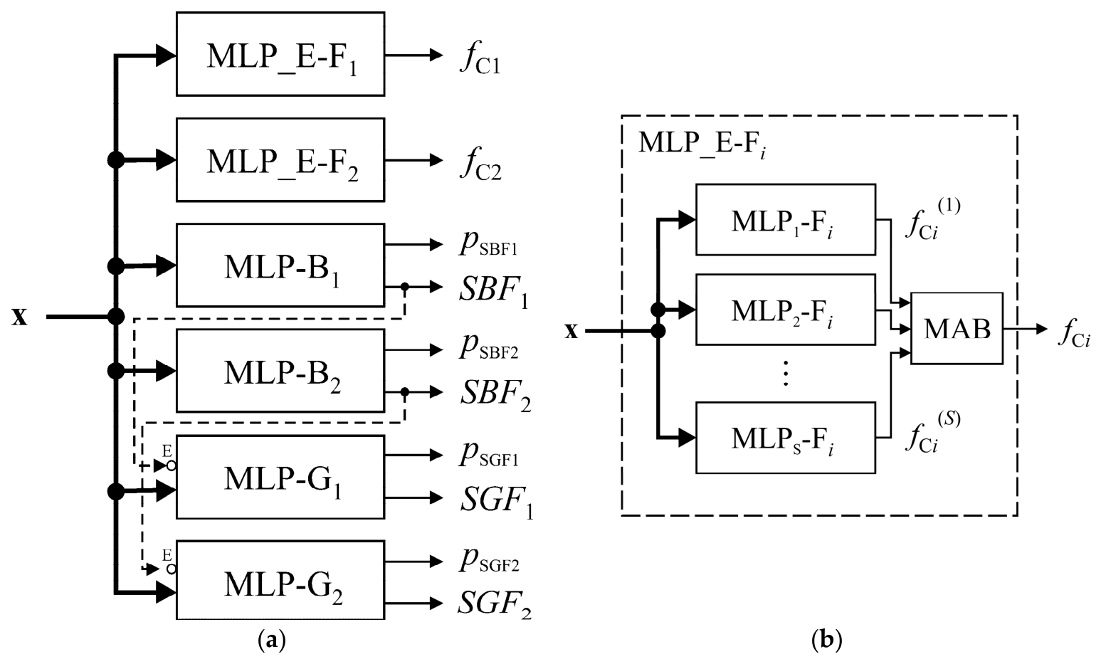
The architecture of the proposed MLP-based DB-CPAC model is shown in Figure 3a. It consists of the following groups of MLP neural network modules: MLP_E-F_i, MLP-B_i and MLP-G_i, where i ∈ {1, 2} denotes the index of the antenna operating band.

The MLP_E-F_i module represents an MLP ensemble consisting of S regression-oriented MLP neural networks with different architectures, denoted as MLP_s-F_i, s ∈ {1, 2, …, S}. All networks within the ensemble are trained using the same training dataset, while the s-th network provides its own estimate of the center frequency of the i-th operating band:

$$f_{\mathrm{C}i}^{(s)}={\mathsf{\Phi }}_{\mathrm{MLP}s-\mathrm{F}i}(x).$$

(7)

The architecture of the MLP_E-F_i ensemble module is shown in Figure 3b. The final estimate of the center frequency of the i-th operating band, denoted by f_Ci, is obtained by averaging the outputs of all ensemble members using the Mean Aggregation Block (MAB), whose transfer function is defined as follows:

$$f_{\mathrm{C}i}={\displaystyle \frac{1}{S}}{\displaystyle \sum _{s=1}^S{f}_{\mathrm{C}i}^{(s)}}.$$

(8)

The MLP-B_i module, containing a classification neural network, is designed to determine whether the normalized bandwidth of the i-th operating band corresponding to the input vector x satisfies the predefined bandwidth criterion. In addition, due to the softmax output layer, the module also provides the posterior probability associated with the positive classification decision:

$${\left[\begin{array}{cc}SB{F}_i& p_{\mathrm{SBFi}i}\end{array}\right]}^{\mathrm{T}}={\mathsf{\Phi }}_{\mathrm{MLP}-\mathrm{B}i}(x).$$

(9)

where SBF_i denotes the bandwidth satisfaction flag associated with the i-th operating band, while p_SBFi = p(SBF_i = 1) represents the estimated probability that the bandwidth criterion is satisfied.

Similarly, the MLP-G_i module, containing a classification neural network, is designed to determine whether the antenna gain at the center frequency of the i-th operating band satisfies the predefined gain criterion for the input vector x. In addition, owing to the softmax output layer, the module also provides the posterior probability associated with the positive classification decision. The output of the MLP-G_i module is expressed as follows:

$${\left[\begin{array}{cc}SG{F}_i& p_{\mathrm{SGFi}}\end{array}\right]}^{\mathrm{T}}={\mathsf{\Phi }}_{\mathrm{MLP}-\mathrm{G}i}(x).$$

(10)

where SGF_i denotes the gain satisfaction flag associated with the i-th operating band, while p_SGFi = p(SGF_i = 1) represents the estimated probability that the gain criterion is satisfied.

The gain estimation is performed only for antenna samples satisfying the bandwidth criterion, which is achieved through the feedback connection of the SBF_i output to the enable input (E) of the MLP-G_i module. Consequently, the MLP-G_i modules solve a conditional classification problem rather than a global classification problem over the entire design space. This hierarchical decision strategy restricts the gain evaluation to antenna geometries that already satisfy the bandwidth requirements, thereby reducing the complexity of the classification task while preserving the effectiveness of the optimization process. In addition, the final top-ranked antenna candidates are verified using full-wave MoM simulations, which further reduce the influence of possible surrogate-model classification errors on the final optimized design.

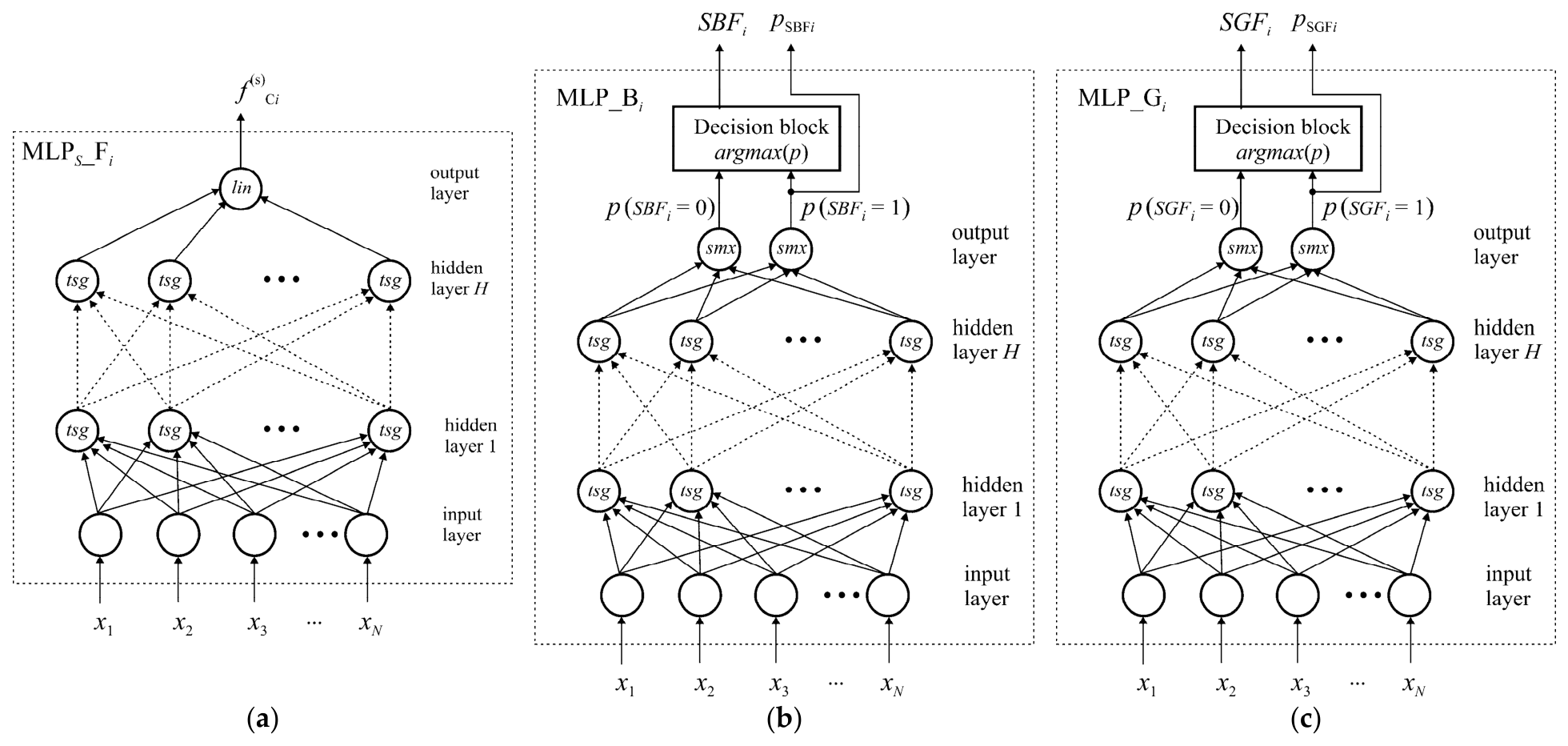
The architectures of the MLP_s-F_i, MLP-B_i and MLP-G_i neural network modules are shown in Figure 4a, Figure 4b, and Figure 4c, respectively. Each module contains an MLP neural network consisting of one input layer, H hidden layers, and one output layer, resulting in a total of L = H + 2 layers. The h-th hidden layer contains n_h neurons, where h ∈ {1, 2, …, H}. The layer index is denoted by l ∈ {1, 2, …, L}, where l = 1 corresponds to the input layer, l = L corresponds to the output layer, while the hidden layers correspond to l = h + l.

The input layer of the MLP network is a buffer layer containing N neurons, where N corresponds to the number of antenna physical parameters, i.e., the dimensionality of the input vector x. In the considered DB-CPAC model, N = 6. Therefore, the output vector of the input layer is given by y¹ = x. The output vectors of all remaining network layers are calculated as follows:

$$y^l=F_l(w^l{y}^{l-1}+b^l) l=2,3,\dots ,L,$$

(11)

where F_l(·) denotes the activation function of the neurons in the l-th layer, w^l is the connection weight matrix between the (l − 1)-th and the l-th layer (the matrix element w^l_i,j represents the connection weight between the j-th neuron of the (l − 1)-th layer and the i-th neuron of the l-th layer), while b^l denotes the bias vector of the l-th layer (the vector element b_i^l represents a bias of the i-th neuron of the l-th layer).

The neurons in the hidden layers employ the hyperbolic tangent sigmoid activation function [16]:

$$F_l(u)={\displaystyle \frac{e^u-e^{-u}}{e^u+e^{-u}}} , l=2,3,\dots ,L-1,$$

(12)

The MLP_s-F_i networks contain a single neuron in the output layer. Its activation function is linear, i.e., F_L(u) = u, resulting in the following output:

$$f_{\mathrm{C}i}=y^L=F_L(w^L{y}^{L-1}+b^L)=w^L{y}^{L-1}+b^L.$$

(13)

On the other hand, the MLP neural networks within the MLP-B_i and MLP-G_i modules contain two neurons in the output layer employing the softmax activation function [16]. For these networks, the input vector of the output layer is given by the following:

$$u^L=w^L{y}^{L-1}+b^L,$$

(14)

where u_j^L denotes the input signal of the j-th neuron in the output layer. The softmax activation function calculates the posterior probabilities of the corresponding output classes according to the following for the MLP network within the MLP-B_i module (Equation (15)) and within the MLP-G_i module (Equation (16)):

$$p(SB{F}_i=j)={\displaystyle \frac{e^{u_j^L}}{e^{u_0^L}+e^{u_1^L}}}, j\in \left\{0,1\right\},$$

(15)

$$p(SG{F}_i=j)={\displaystyle \frac{e^{u_j^L}}{e^{u_0^L}+e^{u_1^L}}}, j\in \left\{0,1\right\},$$

(16)

In both classification networks, the output layer is followed by a decision block whose task is to determine the final class label using the argmax decision rule. For the MLP network within the MLP-B_i module, the decision rule is defined as follows:

$$SB{F}_i=\arg {\max }_{j\in \left\{0,1\right\}}p(SB{F}_i=j),$$

(17)

while for the MLP network within the MLP-G_i module, it is given by the following:

$$SG{F}_i=\arg {\max }_{j\in \left\{0,1\right\}}p(SG{F}_i=j).$$

(18)

Consequently, the outputs of the MLP-B_i module are expressed as follows:

$${\left[\begin{array}{cc}SB{F}_i& p_{\mathrm{SBF}i}\end{array}\right]}^{\mathrm{T}}={\left[\begin{array}{cc}SB{F}_i& p\left(SB{F}_i=1\right)\end{array}\right]}^{\mathrm{T}}.$$

(19)

where p_SBFi = p(SBF_i = 1) denotes the estimated probability that the bandwidth criterion is satisfied.

Similarly, the outputs of the MLP-G_i module are given by the following:

$${\left[\begin{array}{cc}SG{F}_i& p_{\mathrm{SGF}i}\end{array}\right]}^{\mathrm{T}}={\left[\begin{array}{cc}SG{F}_i& p\left(SG{F}_i=1\right)\end{array}\right]}^{\mathrm{T}}.$$

(20)

where p_SGFi = p(SGF_i = 1) denotes the estimated probability that the gain criterion is satisfied.

The trainable parameters of the employed MLP networks are represented by the weight matrices w², …, w^L, and the bias vectors b², …, b^L, which together form the adaptive parameter set denoted by W. These parameters are iteratively adjusted during the training process in order to model, with the highest possible accuracy, the nonlinear mapping defined by Equation (6). The general notation adopted for the employed MLP architecture is MLPH-n₁-n₂-… n_H.

3.2. Dataset Generation Procedure for the Development of the MLP-Based DB-CPAC Surrogate Model

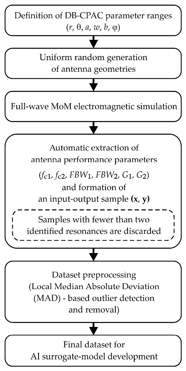
The procedure adopted for generating the dataset used for the development of the proposed MLP-based DB-CPAC surrogate model is summarized in the flowchart shown in Figure 5. Because full-wave MoM simulations are computationally intensive, the dataset generation process can be distributed across multiple independent simulation sessions, each containing a limited number of MoM simulations. After completing all simulation sessions, the final dataset is obtained by merging the samples generated during the individual sessions.

3.3. Training and Validation Procedure of the MLP Networks Constituting the MLP-Based DB-CPAC Model

For the development of the proposed MLP-based DB-CPAC model, including the training, validation, and testing of the MLP networks belonging to all MLP-based modules, an initial dataset U = {(x₁,y₁^D), (x₂,y₂^D), …, (x_s,y_s^D), …, (x_Nu,y_Nu^D)} is generated using the developed DB-CPAC_MoM_Sim software package. Here, y_s^D = [f_C1s^D f_C2s^D SBF_1s^D SBF_2s^D SGF_1s^D SGF_2s^D] denotes the vector of desired output values corresponding to the s-th input vector of antenna physical parameters x_s, while N_U denotes the total number of samples in the dataset.

Prior to the generation of the dataset U, it is necessary to define the variation ranges of the antenna physical parameters, i.e., the set of range boundaries for each input parameter R = {[r_min, r_max], [θ_min, θ_max], [a_min, a_max], [w_min, w_max], [b_min, b_max], [φ_min, φ_max]}. Furthermore, from the input variable space bounded by the parameter value limits R, samples representing invalid antenna geometries must be excluded. Such cases occur when the feed point is located too close to the antenna slot or within the slot itself. These instances are eliminated by introducing supplementary conditions that the values of b and φ must satisfy during sample generation. These conditions are as follows:

$$b\le a_{in}-b^m \wedge \phi \ge {\displaystyle \frac{\theta }{2}}+{\phi }^m \wedge \phi \le -{\displaystyle \frac{\theta }{2}}-{\phi }^m,$$

(21)

where the values b^m and φ^m represent the safety margins for the parameters b and φ, respectively.

Furthermore, since the MoM-based EM simulator provides real-valued bandwidths and gains corresponding to the operating bands of the antenna, threshold values FBW_1min, FBW_2min, G_1min and G_2min also must be defined before constructing the dataset U. Depending on these threshold values and the corresponding values generated by the EM simulator, the variables SBF_1s^D, SBF_2s^D, SGF_1s^D and SGF_2s^D take binary values “0” or “1”.

By selecting the appropriate output variable y and its desired values y_s^D from the vector y_s^D, mutually disjoint training P, validation V, and test T sets corresponding to the currently developed MLP module are formed, having the following formats: P = {(x₁,y₁^D), (x₂,y₂^D), …, (x_s,y_s^D), …, (x_Np,y_Np^D)}; V = {(x₁,y₁^D), (x₂,y₂^D), …, (x_s,y_s^D), …, (x_Nv,y_Nv^D)}; and T = {(x₁,y₁^D), (x₂,y₂^D), …, (x_s,y_s^D), …, (x_Nt,y_Nt^D)}. Here, N_P, N_V, and N_T denote the numbers of samples in the training, validation, and test sets, respectively.

Table 1. Selection of the output variable to form the training, validation, and test set.

Selected MLP-Based Module	MLP_E-F1	MLP_E-F2	MLP-B1	MLP-B2	MLP-G1	MLP-G2
Selected output variable (y)	fC1	fC2	SBF1	SBF2	SGF1	SGF2

summarizes the selection of the output variable y used for the formation of the corresponding training, validation, and test sets according to the type of the MLP-based module being developed. For the development of the MLP_E-F_i and MLP-B_i modules, all samples from the dataset U are used. On the other hand, for the development of the MLP-G_i modules, only those samples satisfying the bandwidth criterion are used, i.e., samples for which SBF_1s^D = 1 and SBF_2s^D = 1.

The training of the MLP networks constituting the proposed DB-CPAC model was performed by the Levenberg–Marquardt training algorithm [16] combined with the Early Stopping method based on the validation set. During the training process, the trainable parameters of the MLP network, collected in the parameter set W, are iteratively updated to minimize the mean squared error (MSE) of the network output relative to the desired values over the training set, denoted by E_P(W) and calculated as follows:

$$E_P\left(W\right)={\displaystyle \frac{1}{2N_P}}{\displaystyle \sum _{s=1}^{N_P}{\left(y_s-y_s^D\right)}^2}.$$

(22)

In parallel with the training process, the MSE evaluated over the validation set, denoted by E_V(W), is continuously monitored and calculated as follows:

$$E_V\left(W\right)={\displaystyle \frac{1}{2N_V}}{\displaystyle \sum _{s=1}^{N_{\mathrm{V}}}{\left(y_s-y_s^D\right)}^2}.$$

(23)

During the initial phase of training, the validation error E_V(W) usually decreases together with the training error. However, after a certain number of training iterations, overfitting effects may occur, causing the validation error to increase despite the continued decrease in the training error. To prevent overfitting and degradation of the network generalization capability, the Early Stopping method is employed. If the validation error E_V(W) fails to decrease during a predefined number of consecutive validation checks denoted by MVF (maximum validation failures), the training process is terminated since the minimum validation error, E_V,min = min E_V(W), is assumed to be already reached, while any further training may lead to overfitting and degradation of the network generalization capability. Consequently, the optimized values of the parameter set W are those corresponding to the minimum validation error, E_V,min [16]. The training process is also terminated if the maximum number of training iterations N_Imax is reached.

For the construction of the proposed MLP-based DB-CPAC model, MLP networks with two hidden layers and an equal but variable number of neurons in both hidden layers were employed. In order to realize MLP-based modules with the highest possible accuracy, MLP networks having different MLP2-n₁-n₂ architectures were trained, where n₁ = n₂ = n, n ∈ [8, 25]. An architecture with exactly two hidden layers was selected to optimally balance model capacity and generalization. While a single layer requires an excessive number of neurons to map highly nonlinear electromagnetic behaviors, deeper networks are prone to overfitting and demand prohibitively large MoM-generated training datasets. Two layers provide sufficient hierarchical feature extraction, ensuring high prediction accuracy without requiring massive computational resources.

Random initial values of the network weights and biases were used during the training process. Since these initial values significantly influence the convergence properties of the training algorithm and the final obtained minimum of the error function, the training procedure for each considered MLP architecture was repeated three times using different random initializations. Among the three independently trained networks having the same architectures, the network yielding the minimum validation MSE at the end of the training process was selected as the representative trained MLP network of that architecture and was subsequently used during the testing procedure.

3.4. Testing Procedure of the MLP Networks Constituting the MLP-Based DB-CPAC Model

The testing procedure using the test set T is performed in order to evaluate the generalization capabilities of the trained MLP networks that are candidates for the realization of the corresponding MLP-based modules of the proposed DB-CPAC model, as well as to select the MLP network architecture expected to provide the highest modeling accuracy for the considered module.

In the testing procedure of the regression-oriented MLP networks intended for the realization of the MLP_E-F_i modules, the following performance metrics were employed: Pearson’s product-moment correlation coefficient (r^PPM) and root mean square error (RMSE) [16].

Pearson’s product-moment correlation coefficient is calculated as follows:

$$r^{PPM}={\displaystyle \frac{{\displaystyle \sum _{p=1}^{N_T}\left(f_{Ci}\left(x_p,W\right)-\overline{f_{Ci}}\right)\cdot \left(f_{Ci,p}^D-\overline{f_{Ci}^D}\right)}}{\sqrt{\left[{\displaystyle \sum _{p=1}^{N_T}{\left(f_{Ci}\left(x_p,W\right)-\overline{f_{Ci}}\right)}^2}\right]\cdot \left[{\displaystyle \sum _{p=1}^{N_T}{\left(f_{Ci,p}^D-\overline{f_{Ci}^D}\right)}^2}\right]}}},$$

(24)

where N_T is the total number of samples in the test set, f_Ci (x_p, W) is the output of the MLP_E-F_i module for the input sample x_p, $f_{Ci,p}^D$ is the desired value of the network output for the sample x_p. $\overline{f_{Ci}}={\displaystyle \frac{1}{N_T}}{\displaystyle \sum _{p=1}^{N_T}{f}_{Ci}\left(x_p,W\right)}$ is the average value of neural network output and ${\overline{f_{Ci}}}^D={\displaystyle \frac{1}{N_T}}{\displaystyle \sum _{p=1}^{N_T}{f}_{Ci,p}^D}$ is the average value of the desired output values.

The RMSE value of the output of the neural network on the test set is defined as follows:

$$RMSE=\sqrt{{\displaystyle \frac{1}{N_T}}{\displaystyle \sum _{p=1}^{N_T}{(f_{Ci}\left(x_p,W\right)-f_{Ci,p}^D)}^2}}.$$

(25)

Similarly, in the testing procedure of the classification-oriented MLP networks intended for the realization of the MLP-B_i and MLP-G_i modules, a general classification performance metric is used. The classification quality is measured by the ability of the classifier—in this case, an ANN—to correctly determine the class membership of an input sample. In order to define the metric for assessing classification quality, it is necessary to define the types of classification outcomes, which are: True Positive (TP)—correctly classified as belonging to the class; False Positive (FP)—does not belong to the class, but is classified as belonging to the class; True Negative (TN)—correctly classified as not belonging to the class; and False Negative (FN)—belongs to the class, but is classified as not belonging to the class. The predicted classification outcomes are represented via a confusion matrix, which illustrates the degree of classification accuracy.

Based on the number of outcomes of the corresponding type, the metrics used to evaluate the classification quality are defined. The basic metrics used to assess classification performance are listed below:

Accuracy represents the proportion of the total number of correctly classified samples (both true positives and true negatives) relative to the total number of samples in the test set.

$$Accuracy={\displaystyle \frac{TP+TN}{TP+TN+FP+FN}},$$

(26)

Precision represents the proportion of correctly classified positive samples out of the total number of samples classified as positive (i.e., predicted to belong to the class):

$$Precision={\displaystyle \frac{TP}{TP+FP}},$$

(27)

Recall (sensitivity) represents the ratio of correctly classified positive samples out of the total number of samples that actually belong to the given class:

$$Recall={\displaystyle \frac{TP}{TP+FN}},$$

(28)

Specificity represents the ratio of correctly classified negative samples out of the total number of samples that actually do not belong to the given class:

$$Specificity={\displaystyle \frac{TN}{TN+FP}},$$

(29)

F1-score represents the harmonic mean of Precision and Sensitivity:

$$F1-score={\displaystyle \frac{2\cdot Precision\cdot Recall}{Precision+Recall}}={\displaystyle \frac{2\cdot TP}{2\cdot TP+FP+FN}},$$

(30)

Balanced Accuracy represents the arithmetic mean of Sensitivity and Specificity:

$$Balanced Accurasy={\displaystyle \frac{Recall+Specificity}{2}},$$

(31)

False Positive Rate (FPR), the complement of Specificity, or 1-Specificity, represents the ratio of incorrectly classified negative samples out of the total number of samples that actually do not belong to the given class:

$$FPR={\displaystyle \frac{FP}{FP+TN}},$$

(32)

FNR (False Negative Rate): complement of Recall, which is as follows:

$$FNR={\displaystyle \frac{FN}{FN+TP}},$$

(33)

3.5. LHS-Based Optimizer

The main objective of the proposed LHS-based optimizer is to determine the optimal values of the antenna physical parameters to achieve the desired antenna characteristics, as specified by the output parameters of the proposed antenna model. This ensures that the synthesized antenna architecture satisfies the imposed optimization requirements and provides the required electromagnetic characteristics. In this case, the optimization aims to realize an antenna with dual-band characteristics, where the center frequencies of both operating bands are as close as possible to the target frequencies, while also ensuring satisfactory operating bandwidths and satisfactory antenna gains at the center frequencies of the corresponding operating bands.

The proposed LHS-based optimizer, implemented in the MATLAB development environment, is hybrid in nature as it combines the proposed surrogate MLP-based DB-CPAC model and the EM MoM simulator. The surrogate MLP-based DB-CPAC model is used for rapid identification of the B best combinations of input parameter values that satisfy the imposed optimization requirements. These are then considered as candidate antenna configurations for final verification using the EM MoM simulator and for selection of the optimal antenna geometry providing the best electromagnetic performance.

During the optimization process, candidate antenna configurations are ranked according to the fitness function:

$$\Psi ={(p_{SBF1})}^2\cdot {(p_{SBF2})}^2\cdot p_{SGF1}\cdot p_{SGF2}.$$

(34)

This function is evaluated only for configurations that satisfy the basic optimization constraints expressed in the following:

$$\left|f_{\mathrm{C}i}-f_{\mathrm{C}i}^{des}\right|\le \Delta f_{tol} \wedge SB{F}_i=1 \wedge SG{F}_i=1 , i\in \left\{1,2\right\},$$

(35)

where f_Ci^des denotes the desired center frequency of the i-th operating band specified in the optimization procedure, while Δf_tol represents the maximum allowable deviation of the center frequency predicted by the neural network model from the desired center frequency of the corresponding operating band.

Although the optimized structure considered in this work is a single patch antenna, the adopted fitness Function (34) intentionally assigns a higher priority to bandwidth than to gain because the antenna is intended as a potential element of a future antenna array for 5G applications. In such applications, the operational bandwidth is largely inherited from the individual array element, whereas the overall array radiation-performance level can subsequently be increased by the array factor through the number of elements and their excitation. Consequently, the adopted weighting reflects the design objective of this particular optimization problem and can be readily modified for other antenna design scenarios.

The proposed LHS-based optimizer employs the Latin Hypercube Sampling (LHS) algorithm [27,28] for uniform sampling of the M-dimensional input parameter space. For each x_i, i ∈ {1,…, M} variable, its allowable range, [x_imin, x_imax], is divided into N mutually disjoint intervals of equal length and probability. Subsequently, one random value is selected from each interval, and the values of all variables are combined using random permutations. This approach ensures that the entire input parameter space is covered significantly more uniformly than with pure random sampling.

The operation of the proposed LHS-based optimizer can be summarized through the following steps:

• A total of N_G valid global candidate antenna configurations satisfying Condition (21) are generated within the input parameter space bounded by the variable limits defined in set R.
• Each candidate antenna configuration is evaluated using the proposed MLP-based DB-CPAC model.
• A candidate antenna configuration passes the global exploration phase if it satisfies Condition (35).
• For all candidates satisfying the imposed constraints, the fitness function value ψ is calculated using (34).
• The candidates are sorted based on their fitness function values, and the B best-ranked candidates are selected as seed candidates for the first local refinement phase.
• Around each of the selected B seed candidates, N_L1 local candidate configurations are generated within a neighborhood corresponding to ±10% of the global search range.
• The generated local candidates are evaluated using the proposed MLP-based DB-CPAC model, and those satisfying Condition (35) are added to the candidate set.
• Subsequently, all currently accepted candidate configurations are sorted based on their fitness function values, and the B best-ranked candidates are selected as seed candidates for the second local refinement phase.
• Around each of the newly selected B seed candidates, N_L2 local candidate configurations are generated within a narrower neighborhood corresponding to ±5% of the global search range.
• Finally, all candidate configurations satisfying the constraints from the global and both local refinement phases are merged into a single set. After removing duplicate solutions, the remaining candidates are ranked based on their fitness function values, and the top B antenna geometry proposals are selected.
• In the final optimization step, these B selected geometry proposals are verified using the EM MoM simulator. The optimal antenna geometry is then chosen as the one providing the widest operating bandwidth (primary optimization criterion) while simultaneously achieving the highest possible antenna gain at the center frequencies of the operating bands (secondary optimization criterion).

The acceleration of the optimization process achieved by the proposed hybrid MLP–MoM LHS-based optimization approach, compared to the conventional “pure” EM MoM optimization procedure using the same LHS strategy, can be approximately estimated as follows [23]:

$$A_{MoM}^{MLP-MoM}={\displaystyle \frac{(N_G+B{N}_{L1}+B{N}_{L2})\cdot T_{MoM}}{(N_G+B{N}_{L1}+B{N}_{L2})\cdot T_{MLP\_DP-CPAC}+B{T}_{MoM}}},$$

(36)

where T_MoM and T_{MLP_DP-CPAC} denote the computation times required to evaluate the modeled antenna characteristics for a single combination of physical parameters using the EM MoM simulator and the proposed MLP-based DB-CPAC model, respectively.

It should be noted that the acceleration factor defined by Equation (36) refers exclusively to the online optimization stage. The computational cost associated with generating the training dataset and training the MLP surrogate model represents a one-time offline investment, after which the trained model can be reused for multiple optimization tasks within the considered design space. Even when this offline cost is considered, the number of full-wave MoM simulations required to generate the training database is substantially smaller than the number of MoM simulations required by a conventional pure-MoM optimization run using the same sampling strategy. Consequently, this offline cost is amortized over all subsequent optimization runs, while the acceleration factor given by Equation (36) remains applicable to each individual optimization run.

4. Results and Discussion

The proposed surrogate MLP-based DB-CPAC model is employed for the modeling and optimization of a dual-band circular patch antenna with a C-shaped slot, designed on an FR4 substrate with a thickness of h = 1.6 mm, a relative dielectric permittivity of ε_r = 4.8 and a loss tangent of tan δ = 0.026.

The model is developed to accommodate various physical antenna configurations, ensuring that the lower operating band covers the 2.4–2.8 GHz frequency range (encompassing the 5G NR n41 band), while the higher operating band spans the 3.3–3.9 GHz range to include the widely used 5G NR n78 band. Within these specified ranges, the antenna is intended for operation across selected channel allocations.

4.1. Results of Training and Testing of the MLP-Based DB-CPAC Model

The training of the proposed MLP-based DB-CPAC model is conducted by training a large number of MLP neural networks for each module separately, following the procedure detailed in Section 3.3.

By utilizing the developed DB-CPAC_MoM_Sim software package, following the dataset generation and preprocessing procedure described in Section 3.2, and employing uniform random (Monte Carlo) sampling within the input parameter space defined in

Table 2. Boundaries of the input variable space.

Input Variable Ranges	[rmin, rmax] [mm]	[θmin, θmax] [°]	[amin, amax] [mm]	[wmin, wmax] [mm]	[bmin, bmax] [mm]	[φmin, φmax] [°]
Values	[12, 16]	[80, 160]	[4.8, 14.22]	[0.36, 4.8]	[2.4, 9.6]	[0, 360]

, a dataset (U) comprising 6897 valid antenna samples was generated. This sampling strategy was adopted based on our previous investigations, which demonstrated that uniformly distributed random sampling can provide an effective training dataset for antenna surrogate modeling and can lead to better neural-network generalization than conventional uniform-grid sampling for the same number of full-wave electromagnetic simulations [23,24]. It should be noted that the LHS was not used for training-dataset generation, but only during the subsequent LHS-based optimization stage. Although uniform random sampling does not provide the same stratification properties as LHS and may lead to locally sparse regions in high-dimensional spaces, the obtained validation and test results indicate that the generated dataset provides sufficiently representative coverage for the considered optimization problem. During the dataset generation process, the following threshold values were adopted: FBW_1min = 0.02, FBW_2min = 0.02, G_1min = 3 dBi, and G_2min = 3 dBi.

To reduce the overall execution time, the database was generated through 24 independent simulation sessions, each comprising up to 500 MoM simulations, executed at different time periods on four computers with different computational capabilities operating in parallel. The final dataset was obtained by merging the samples generated during all simulation sessions.

From the dataset (U) containing 6897 samples, the training (P), validation (V), and testing (T) datasets—comprising 5276, 931, and 690 samples, respectively—are formed for the MLP neural networks belonging to the MLP_E-Fi and MLP-Bi modules. Following the selection of samples from the dataset (U) that satisfy the SBF₁^D = 1 condition, the datasets (P), (V), and (T), containing 1365, 241, and 188 samples, respectively, are generated for the networks within the MLP-G₁ module. Similarly, after isolating the samples from the dataset (U) that fulfill the SBF₂^D = 1 condition, the corresponding datasets (P), (V), and (T), consisting of 1737, 307, and 221 samples, respectively, are established for the MLP-G₂ module.

All MLP2-n-n, n ∈ [8, 25], neural networks are trained using the Levenberg–Marquardt learning algorithm. During the training process, the maximum number of validation failures is set to MVF = 15, while the maximum number of training iterations is limited to N_Imax = 5000.

Table 3. Values of the Pearson product-moment correlation coefficient (r^PPM) and root mean square error (RMSE) obtained on the test and validation datasets for the ten best-performing MLP neural networks trained for the estimation of f_C1.

Neural Networks	Test Set		Validation Set
	rPPM	RMSE [GHz]	rPPM	RMSE [GHz]
MLP2-16-16	0.9879	0.0371	0.9897	0.0324
MLP2-24-24	0.9878	0.0372	0.9890	0.0341
MLP2-19-19	0.9875	0.0376	0.9874	0.0357
MLP2-11-11	0.9871	0.0382	0.9835	0.0408
MLP2-20-20	0.9868	0.0387	0.9895	0.0335
MLP2-23-23	0.9866	0.0389	0.9874	0.0362
MLP2-22-22	0.9863	0.0394	0.9877	0.0367
MLP2-14-14	0.9862	0.0395	0.9882	0.0366
MLP2-25-25	0.9860	0.0397	0.9889	0.0346
MLP2-17-17	0.9859	0.0399	0.9848	0.0386

summarizes the values of the Pearson product-moment correlation coefficient (r^PPM) and the root mean square error (RMSE) obtained on the validation and test datasets for the ten best-performing MLP neural networks trained for the estimation of f_C1. The networks are ranked according to the RMSE achieved on the test dataset. For the implementation of the MLP_E-F₁ module, a three-member ensemble (S = 3) is adopted, consisting of the three neural networks exhibiting the lowest RMSE values on the test dataset, namely MLP2-16-16, MLP2-24-24, and MLP2-19-19.

Similarly,

Table 4. Values of the Pearson product-moment correlation coefficient (r^PPM) and root mean square error (RMSE) obtained on the test and validation datasets for the ten best-performing MLP neural networks trained for the estimation of f_C2.

Neural Networks	Test Set		Validation Set
	rPPM	RMSE [GHz]	rPPM	RMSE [GHz]
MLP2-13-13	0.9880	0.0583	0.9878	0.0593
MLP2-21-21	0.9875	0.0599	0.9867	0.0626
MLP2-14-14	0.9871	0.0606	0.9887	0.0577
MLP2-12-12	0.9869	0.0610	0.9868	0.0610
MLP2-23-23	0.9865	0.0631	0.9867	0.0630
MLP2-17-17	0.9821	0.0712	0.9875	0.0608
MLP2-25-25	0.9810	0.0737	0.9866	0.0629
MLP2-19-19	0.9796	0.0760	0.9871	0.0605
MLP2-22-22	0.9772	0.0811	0.9888	0.0590
MLP2-15-15	0.9765	0.0821	0.9833	0.0699

presents the values of the r^PPM and RMSE obtained on the validation and test datasets for the ten best-performing MLP neural networks trained for the estimation of f_C2. For the implementation of the MLP_E-F₂ module, a three-member ensemble (S = 3) is selected, consisting of the MLP2-13-13, MLP2-21-21, and MLP2-14-14 neural networks, which achieved the lowest RMSE values on the test dataset.

The testing results of the ensemble neural networks implementing the MLP_E-F₁ and MLP_E-F₂ modules are summarized in

Table 5. Testing results of the ensemble neural networks implementing the MLP_E-F₁ and MLP_E-F₂ modules.

Neural Networks	fci	Test Set
		rPPM	RMSE [GHz]
[MLP2-16-16, MLP2-24-24, MLP2-19-19]	fc1	0.9902	0.0333
[MLP2-13-13, MLP2-21-21, MLP2-14-14]	fc2	0.9924	0.0464

. The RMSE values obtained for both modules are approximately 33 MHz and 46 MHz, respectively, demonstrating the high prediction accuracy of the proposed modular framework.

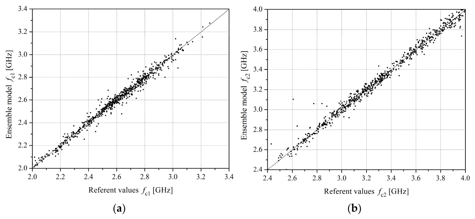
The scatter plots corresponding to the ensemble neural networks implementing the MLP_E-F₁ and MLP_E-F₂ modules are shown in Figure 6a and Figure 6b, respectively. In both figures, a very good agreement between the center frequencies predicted by the ensemble neural networks and the corresponding reference values obtained by the EM MoM simulator is observed. This further confirms the high accuracy and generalization capability of the proposed MLP_E-F₁ and MLP_E-F₂ modules.

Table 6. Classification performance metrics obtained for the ten best-performing MLP neural networks implementing the MLP-B₁ module.

Neural Networks	Test Set								Validation Set
	Acc	Prec	Recall	Spec	F1	BalAcc	FPR	FNR	Acc	Prec	Recall	Spec	F1	BalAcc	FPR	FNR
MLP2-8-8	0.9304	0.8784	0.9028	0.9430	0.8904	0.9229	0.0570	0.0972	0.9388	0.9058	0.8897	0.9600	0.8977	0.9248	0.0400	0.1103
MLP2-11-11	0.9275	0.8990	0.8657	0.9557	0.8821	0.9107	0.0443	0.1343	0.9334	0.9011	0.8754	0.9585	0.8881	0.9170	0.0415	0.1246
MLP2-9-9	0.9261	0.9104	0.8472	0.9620	0.8777	0.9046	0.0380	0.1528	0.9356	0.9077	0.8754	0.9615	0.8913	0.9185	0.0385	0.1246
MLP2-15-15	0.9217	0.8932	0.8519	0.9536	0.8720	0.9027	0.0464	0.1481	0.9184	0.8727	0.8541	0.9462	0.8633	0.9001	0.0538	0.1459
MLP2-14-14	0.9203	0.8779	0.8657	0.9451	0.8718	0.9054	0.0549	0.1343	0.9205	0.8683	0.8683	0.9431	0.8683	0.9057	0.0569	0.1317
MLP2-24-24	0.9188	0.8774	0.8611	0.9451	0.8692	0.9031	0.0549	0.1389	0.8990	0.8476	0.8114	0.9369	0.8291	0.8742	0.0631	0.1886
MLP2-10-10	0.9159	0.8496	0.8889	0.9283	0.8688	0.9086	0.0717	0.1111	0.9313	0.9004	0.8683	0.9585	0.8841	0.9134	0.0415	0.1317
MLP2-20-20	0.9145	0.8756	0.8472	0.9451	0.8612	0.8962	0.0549	0.1528	0.9119	0.8566	0.8505	0.9385	0.8536	0.8945	0.0615	0.1495
MLP2-19-19	0.9116	0.8605	0.8565	0.9367	0.8585	0.8966	0.0633	0.1435	0.9087	0.8551	0.8399	0.9385	0.8474	0.8892	0.0615	0.1601
MLP2-21-21	0.9116	0.8605	0.8565	0.9367	0.8585	0.8966	0.0633	0.1435	0.9033	0.8448	0.8327	0.9338	0.8387	0.8833	0.0662	0.1673

and

Table 7. Classification performance metrics obtained for the ten best-performing MLP neural networks implementing the MLP-B₂ module.

Neural Networks	Test Set								Validation Set
	Acc	Prec	Recall	Spec	F1	BalAcc	FPR	FNR	Acc	Prec	Recall	Spec	F1	BalAcc	FPR	FNR
MLP2-14-14	0.9072	0.8722	0.8498	0.9365	0.8609	0.8932	0.0635	0.1502	0.9130	0.8845	0.8713	0.9363	0.8778	0.9038	0.0637	0.1287
MLP2-19-19	0.9043	0.8553	0.8627	0.9256	0.8590	0.8941	0.0744	0.1373	0.9108	0.8680	0.8862	0.9246	0.8770	0.9054	0.0754	0.1138
MLP2-16-16	0.9029	0.8705	0.8369	0.9365	0.8534	0.8867	0.0635	0.1631	0.9066	0.8824	0.8533	0.9363	0.8676	0.8948	0.0637	0.1467
MLP2-10-10	0.9014	0.8603	0.8455	0.9300	0.8528	0.8877	0.0700	0.1545	0.9108	0.8838	0.8653	0.9363	0.8744	0.9008	0.0637	0.1347
MLP2-13-13	0.9014	0.8603	0.8455	0.9300	0.8528	0.8877	0.0700	0.1545	0.9012	0.8758	0.8443	0.9330	0.8598	0.8887	0.0670	0.1557
MLP2-21-21	0.8986	0.8622	0.8326	0.9322	0.8472	0.8824	0.0678	0.1674	0.8947	0.8642	0.8383	0.9263	0.8511	0.8823	0.0737	0.1617
MLP2-9-9	0.9000	0.8796	0.8155	0.9431	0.8463	0.8793	0.0569	0.1845	0.9066	0.8871	0.8473	0.9397	0.8668	0.8935	0.0603	0.1527
MLP2-20-20	0.8957	0.8546	0.8326	0.9278	0.8435	0.8802	0.0722	0.1674	0.9001	0.8663	0.8533	0.9263	0.8597	0.8898	0.0737	0.1467
MLP2-8-8	0.8913	0.8496	0.8240	0.9256	0.8366	0.8748	0.0744	0.1760	0.8969	0.8696	0.8383	0.9296	0.8537	0.8840	0.0704	0.1617
MLP2-25-25	0.8913	0.8527	0.8197	0.9278	0.8359	0.8738	0.0722	0.1803	0.9012	0.8829	0.8353	0.9380	0.8585	0.8867	0.0620	0.1647

summarize the classification performance obtained on the test and validation datasets for the MLP neural networks trained to implement the MLP-B₁ and MLP-B₂ modules, respectively, which are tasked with estimating the binary values of SBF₁ and SBF₂. The neural networks are ranked primarily according to their F1-score and secondarily by the Accuracy achieved on the test dataset. This ranking criterion is adopted because the F1-score simultaneously accounts for both Precision and Recall, thereby providing a more informative assessment of classifier performance in the presence of class imbalance. Since the positive class (SBF_i = 1) is of primary importance for the subsequent optimization process, the F1-score serves as a more relevant selection criterion than Accuracy alone.

Based on these results, the MLP2-8-8 neural network is selected to implement the MLP-B₁ module, achieving an accuracy of 93.0% and an F1-score of 89.0% on the test dataset. Similarly, the MLP2-14-14 neural network is selected for the MLP-B₂ module, achieving an accuracy of 90.7% and an F1-score of 86.1%. These outcomes indicate high reliability of the proposed modules in determining the values of SBF₁ and SBF₂.

Table 8. Confusion matrices obtained on the test dataset for (a) the MLP-B₁ module and (b) the MLP-B₂ module.

(a)
MLP-B1	0	1
0	447	27
1	21	195
(b)
MLP-B2	0	1
0	428	39
1	35	198

presents the confusion matrices obtained for the MLP-B₁ and MLP-B₂ modules on the test dataset. It can be observed that the vast majority of samples are correctly classified. Specifically, the MLP-B₁ module correctly classifies 447 negative and 195 positive samples, with only 48 samples being misclassified. Similarly, the MLP-B₂ module correctly classifies 428 negative and 198 positive samples, while 74 samples are misclassified. These results further confirm the strong classification capability and generalization performance of the proposed modular framework.

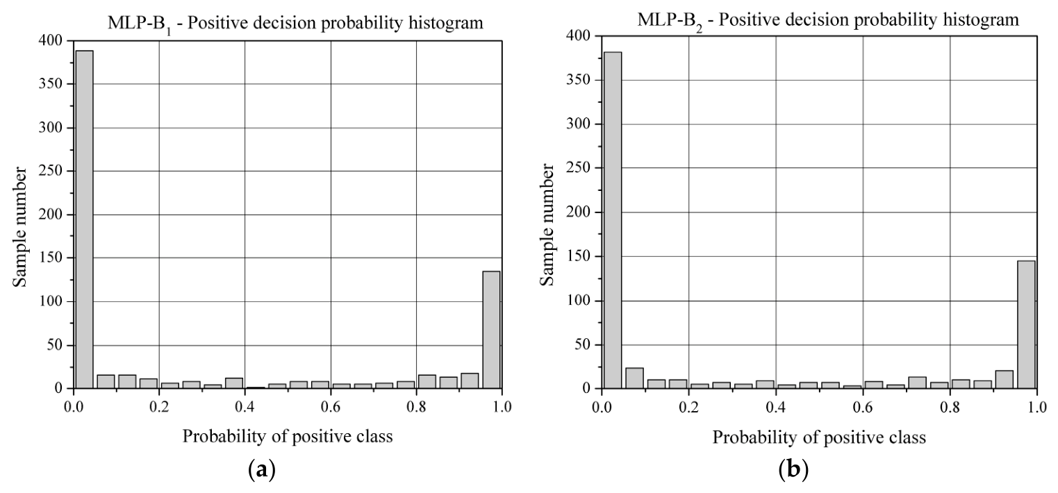
Figure 7a and Figure 7b display the histograms of the posterior probabilities for the positive decision generated by the MLP-B₁ and MLP-B₂ modules, respectively, to determine whether the operational bandwidths FBW₁ and FBW₂ satisfy the required bandwidth criteria expressed through the values of SBF₁ and SBF₂. It can be observed that both histograms exhibit pronounced maxima near probability values of 0 and 1, whereas only a relatively small number of samples are associated with intermediate probability values. This indicates that the proposed MLP classifiers make their decisions with a high degree of confidence, leaving only a small fraction of samples located near the classification boundary. Consequently, the obtained probability estimates can be considered reliable indicators of the confidence associated with the classification decisions.

Table 9. Classification performance metrics obtained for the ten best-performing MLP neural networks implementing the MLP-G₁ module.

Neural Networks	Test Set								Validation Set
	Acc	Prec	Recall	Spec	F1	BalAcc	FPR	FNR	Acc	Prec	Recall	Spec	F1	BalAcc	FPR	FNR
MLP2-14-14	0.8564	0.7544	0.7679	0.8939	0.7611	0.8309	0.1061	0.2321	0.7759	0.5733	0.6615	0.8182	0.6143	0.7399	0.1818	0.3385
MLP2-21-21	0.8617	0.8125	0.6964	0.9318	0.7500	0.8141	0.0682	0.3036	0.7925	0.6271	0.5692	0.8750	0.5968	0.7221	0.1250	0.4308
MLP2-12-12	0.8511	0.7500	0.7500	0.8939	0.7500	0.8220	0.1061	0.2500	0.7967	0.6212	0.6308	0.8580	0.6260	0.7444	0.1420	0.3692
MLP2-8-8	0.8351	0.6923	0.8036	0.8485	0.7438	0.8260	0.1515	0.1964	0.7842	0.5783	0.7385	0.8011	0.6486	0.7698	0.1989	0.2615
MLP2-18-18	0.8404	0.7241	0.7500	0.8788	0.7368	0.8144	0.1212	0.2500	0.7925	0.6027	0.6769	0.8352	0.6377	0.7561	0.1648	0.3231
MLP2-22-22	0.8457	0.7547	0.7143	0.9015	0.7339	0.8079	0.0985	0.2857	0.7759	0.5821	0.6000	0.8409	0.5909	0.7205	0.1591	0.4000
MLP2-15-15	0.8457	0.7647	0.6964	0.9091	0.7290	0.8028	0.0909	0.3036	0.8091	0.6301	0.7077	0.8466	0.6667	0.7771	0.1534	0.2923
MLP2-24-24	0.8298	0.7000	0.7500	0.8636	0.7241	0.8068	0.1364	0.2500	0.8050	0.6216	0.7077	0.8409	0.6619	0.7743	0.1591	0.2923
MLP2-9-9	0.8298	0.7143	0.7143	0.8788	0.7143	0.7965	0.1212	0.2857	0.8008	0.6197	0.6769	0.8466	0.6471	0.7618	0.1534	0.3231
MLP2-11-11	0.8298	0.7308	0.6786	0.8939	0.7037	0.7863	0.1061	0.3214	0.8008	0.6308	0.6308	0.8636	0.6308	0.7472	0.1364	0.3692

and

Table 10. Classification performance metrics obtained for the ten best-performing MLP neural networks implementing the MLP-G₂ module.

Neural Networks	Test Set								Validation Set
	Acc	Prec	Recall	Spec	F1	BalAcc	FPR	FNR	Acc	Prec	Recall	Spec	F1	BalAcc	FPR	FNR
MLP2-18-18	0.7828	0.7951	0.8083	0.7525	0.8017	0.7804	0.2475	0.1917	0.7720	0.7622	0.8443	0.6857	0.8011	0.7650	0.3143	0.1557
MLP2-23-23	0.7828	0.8000	0.8000	0.7624	0.8000	0.7812	0.2376	0.2000	0.7785	0.7797	0.8263	0.7214	0.8023	0.7739	0.2786	0.1737
MLP2-22-22	0.7783	0.7886	0.8083	0.7426	0.7984	0.7755	0.2574	0.1917	0.7622	0.7701	0.8024	0.7143	0.7859	0.7583	0.2857	0.1976
MLP2-21-21	0.7692	0.7674	0.8250	0.7030	0.7952	0.7640	0.2970	0.1750	0.7687	0.7500	0.8623	0.6571	0.8022	0.7597	0.3429	0.1377
MLP2-8-8	0.7511	0.7444	0.8250	0.6634	0.7826	0.7442	0.3366	0.1750	0.7655	0.7411	0.8743	0.6357	0.8022	0.7550	0.3643	0.1257
MLP2-17-17	0.7602	0.7724	0.7917	0.7228	0.7819	0.7572	0.2772	0.2083	0.7655	0.7778	0.7964	0.7286	0.7870	0.7625	0.2714	0.2036
MLP2-11-11	0.7511	0.7481	0.8167	0.6733	0.7809	0.7450	0.3267	0.1833	0.7655	0.7654	0.8204	0.7000	0.7919	0.7602	0.3000	0.1796
MLP2-25-25	0.7466	0.7388	0.8250	0.6535	0.7795	0.7392	0.3465	0.1750	0.7720	0.7594	0.8503	0.6786	0.8023	0.7644	0.3214	0.1497
MLP2-19-19	0.7466	0.7424	0.8167	0.6634	0.7778	0.7400	0.3366	0.1833	0.7752	0.7606	0.8563	0.6786	0.8056	0.7674	0.3214	0.1437
MLP2-10-10	0.7511	0.7559	0.8000	0.6931	0.7773	0.7465	0.3069	0.2000	0.7752	0.7882	0.8024	0.7429	0.7953	0.7726	0.2571	0.1976

summarize the classification performance obtained on the test and validation datasets for the MLP neural networks trained to implement the MLP-G₁ and MLP-G₂ modules, respectively. These modules are responsible for estimating the binary values of SGF₁ and SGF₂, which indicate whether the antenna gains at the center frequencies of the first and second operating bands satisfy the predefined criteria G_1min and G_2min, respectively. Similar to the MLP-Bi modules, the neural networks are ranked primarily according to the F1-score and secondarily according to the Accuracy achieved on the test dataset. Since the positive class (SGFi = 1) represents antenna configurations satisfying the gain requirements and is therefore of primary importance for the optimization process, the F1-score is adopted as the principal performance indicator.

Based on the obtained results, the MLP2-14-14 neural network is selected for the implementation of the MLP-G₁ module, achieving an accuracy of 85.6% and an F1-score of 76.1% on the test dataset. For the implementation of the MLP-G₂ module, the MLP2-18-18 neural network is selected, achieving an Accuracy of 78.3% and an F1-score of 80.2% on the test dataset. Although the obtained classification performance is slightly lower than that achieved by the MLP-B₁ and MLP-B₂ modules, gain classification represents a significantly more challenging problem due to the stronger nonlinear dependence of the antenna radiation characteristics on its physical parameters. Furthermore, the MLP-G₁ and MLP-G₂ modules are not utilized as standalone decision-making components; instead, they are activated only for antenna configurations that have already satisfied the bandwidth-related criteria evaluated by the MLP-B₁ and MLP-B₂ modules. Consequently, these modules constitute an additional filtering stage within the hierarchical architecture of the proposed surrogate model, thereby reducing the impact of their classification errors on the overall optimization process.

Table 11. Confusion matrices obtained on the test dataset for (a) the MLP-G₁ module and (b) the MLP-G₂ module.

(a)
MLP-G1	0	1
0	118	14
1	13	43
(b)
MLP-G2	0	1
0	76	25
1	23	97

presents the confusion matrices obtained for the MLP-G₁ and MLP-G₂ modules on the test dataset. It can be observed that the majority of samples are correctly classified. Specifically, the MLP-G₁ module correctly classifies 118 negative and 43 positive samples, while producing only 27 false-positive and 13 false-negative decisions. Similarly, the MLP-G₂ module correctly classifies 76 negative and 97 positive samples, with 25 false-positive and 23 false-negative decisions observed. These results confirm that the proposed modules are capable of reliably identifying antenna configurations that satisfy the specified gain requirements.

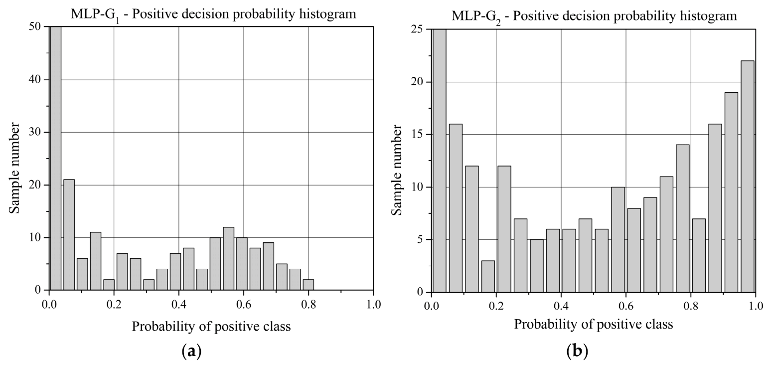
Figure 8a and Figure 8b show the histograms of the posterior probabilities of the positive class generated by the MLP-G₁ and MLP-G₂ modules, respectively. Compared with the corresponding histograms obtained for the MLP-B_i modules, a larger number of samples exhibit intermediate probability values, indicating a higher degree of uncertainty in the classification process. This behavior is expected since gain is generally more difficult to predict than bandwidth-related characteristics. Nevertheless, the histograms still exhibit noticeable concentrations of samples near the probability extremes, demonstrating that a substantial portion of classification decisions is made with a relatively high level of confidence.

It should also be emphasized that the posterior probabilities generated by the MLP-G_i modules are not used solely for binary decision making. Instead, they are directly incorporated into the fitness function employed by the LHS-based optimizer. Consequently, antenna configurations associated with uncertain classification outcomes are naturally assigned lower fitness values, while configurations producing highly confident positive decisions are favored. Therefore, the optimization process inherently suppresses ambiguous candidates and promotes antenna geometries for which the surrogate model exhibits a higher degree of confidence, further increasing the reliability of the obtained optimization results.

4.2. Comparative Evaluation of the Proposed MLP-Based DB-CPAC Surrogate Model Using Alternative AI-Based Surrogate Models

To further validate the proposed MLP-based surrogate model, its performance was compared with two widely used alternative AI-based surrogate models, namely optimized Gaussian Support Vector Regression (SVR) and Random Forest (RF), both developed using exactly the same training and test datasets. Since the prediction of the two center frequencies represents the principal regression task of the proposed surrogate model, whereas the remaining outputs correspond to binary classification problems, the comparison was intentionally limited to the regression component of the proposed methodology.

The training settings of the alternative surrogate models are summarized in

Table 12. Training configuration of the alternative AI-based surrogate models used for comparative evaluation.

Parameter	Optimized SVR	Random Forest
Learning algorithm	Gaussian SVR	Bagged trees
Hyperparameter optimization	Bayesian	None
Objective evaluations	40	-
Cross-validation	5-fold	-
Kernel	Gaussian	-
Box Constraint	fc1: 1.129465, fc2: 226.189181	-
Kernel Scale	fc1: 0.615355, fc2: 0.419609	-
Epsilon	fc1: 0.003172, fc2: 0.022796	-
Number of Trees	-	300
Minimum Leaf Size	-	5

. The optimized Gaussian SVR employed a Gaussian kernel together with Bayesian hyperparameter optimization using 40 objective evaluations and 5-fold cross-validation. The optimized hyperparameters included the Box Constraint, Kernel Scale, and Epsilon, whose final values are listed in Table 12 for both center-frequency prediction models. The Random Forest benchmark was implemented as a bagged ensemble consisting of 300 regression trees with a minimum leaf size of 5. The random number generator was initialized using rng(1,’twister’).

The comparison results are summarized in

Table 13. Performance comparison of the proposed MLP-based DB-CPAC surrogate model and alternative AI-based DB-CPAC surrogate models.

Model	Development Time [s]	Inference Time [ms/Sample]	fc1		fc2
			rPPM	RMSE [GHz]	rPPM	RMSE [GHz]
Proposed MLP-based	274.78	0.030	0.9902	0.0333	0.9924	0.0464
Optimized Gaussian SVR	8729.75	0.060	0.9711	0.0570	0.9506	0.1174
Random Forest	6.20	0.334	0.9580	0.0738	0.9369	0.1397

, which reports the prediction accuracy together with the model development and inference times for all considered surrogate models. For the proposed MLP-based surrogate model, the reported development time represents the total time required to develop the complete surrogate-model architecture, including the training of all neural networks forming the ensemble model as well as the binary classification models used for predicting the existence of the lower and upper operating bands and the corresponding realized gains. For the optimized Gaussian SVR model, the reported development time includes both the Bayesian hyperparameter optimization procedure and the training of the final surrogate model. For the Random Forest model, the reported time corresponds to the complete development of the bagged tree-based surrogate model.

As can be observed from Table 13, the proposed MLP-based surrogate model consistently achieved the highest prediction accuracy for both center frequencies, yielding the lowest RMSE and the highest r^PPM values among all evaluated surrogate models. In addition, despite its considerably more sophisticated architecture, the proposed surrogate model required approximately 32 times less development time than the optimized Gaussian SVR model employing Bayesian hyperparameter optimization. Although the Random Forest model required only a few seconds for development, this reduction in computational cost was achieved at the expense of a noticeable degradation in prediction accuracy. Furthermore, the proposed MLP-based surrogate model exhibited the shortest inference time, making it particularly suitable for surrogate-assisted iterative antenna optimization, where thousands of model evaluations are typically required.

4.3. Results Obtained by the Hybrid Surrogate MLP–MoM Antenna Optimization Approach

The effectiveness of the proposed hybrid surrogate MLP–MoM optimization framework employing the developed MLP-based DB-CPAC model is demonstrated through the optimization of the antenna physical parameters. The optimization objective is to obtain antenna configurations whose operating bands are centered at f_C1 = 2.6 GHz and f_C2 = 3.6 GHz, while simultaneously ensuring satisfactory bandwidths and gains across both operational bands. The following LHS optimizer parameters are utilized throughout the MLP optimization process: N_G = 500,000, N_L1 = 100, N_L2 = 100, and B = 10.

Table 14. Antenna physical parameters, posterior probabilities, and fitness-function values of the ten highest-ranked antenna candidates identified by the surrogate MLP-based DB-CPAC optimization procedure.

Ranking	Antenna Configurations (Physical Parameters)						Posterior Probabilities				ψ
	r [mm]	θ [°]	a [mm]	w [mm]	b [mm]	φ [°]	pSBF1	pSBF2	pSGF1	pSGF2
1	15.26	122.70	11.11	4.15	6.46	76.09	0.99998	0.95210	0.67726	0.97395	0.59791
2	15.28	120.15	11.15	4.14	6.77	73.36	0.99998	0.92257	0.68934	0.94628	0.55518
3	15.33	121.36	11.07	4.16	6.56	71.63	0.99997	0.90801	0.70158	0.95036	0.54970
4	15.24	122.47	10.82	3.97	6.55	77.00	0.99998	0.94793	0.64039	0.93799	0.53973
5	15.20	138.56	10.88	4.20	5.81	76.29	0.99778	0.97896	0.57223	0.97091	0.53009
6	15.09	136.90	10.67	4.03	5.61	73.72	0.99781	0.96625	0.58488	0.96912	0.52688
7	15.26	119.88	11.15	3.89	6.08	68.05	0.99963	0.83441	0.80813	0.90656	0.50971
8	15.12	136.73	10.64	3.99	5.36	73.81	0.99268	0.95504	0.58713	0.96504	0.50925
9	15.01	139.84	10.90	3.99	5.69	79.33	0.99465	0.98131	0.54584	0.97808	0.50861
10	15.33	130.35	10.54	4.02	5.44	76.24	0.99809	0.96177	0.59818	0.90763	0.50029

summarizes the physical parameters of the ten highest-ranked antenna candidates identified exclusively by the surrogate MLP-based DB-CPAC model using the proposed LHS-based optimization procedure. In addition to the antenna physical parameters, the table includes the posterior probabilities generated by the surrogate model and the corresponding fitness function values used for candidate ranking.

The hybrid nature of the proposed optimization framework is introduced only during the final verification stage. Specifically, the ten candidate antenna configurations identified by the surrogate optimization procedure are subsequently analyzed using the conventional EM MoM simulator. The corresponding values of the center frequencies, bandwidths, and gains obtained via EM MoM analysis are then evaluated with respect to the imposed optimization objectives. Consequently, computationally expensive EM MoM simulations are restricted to only ten candidate antenna configurations rather than being performed iteratively throughout the entire optimization process.

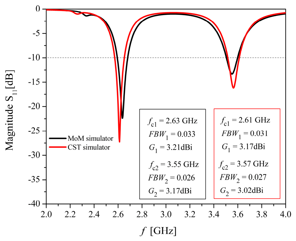
Among the verified antenna configurations, a representative design satisfying all imposed optimization requirements is selected for detailed presentation. The selected antenna geometry is characterized by the following physical parameters: r = 15.33 mm, θ = 121.36°, a = 11.07 mm, w = 4.16 mm, b = 6.56 mm, and φ = 71.63°. The corresponding simulated S₁₁ characteristic obtained by the EM MoM simulator is shown in Figure 9. The resulting antenna characteristics are f_C1 = 2.63 GHz, f_C2 = 3.55 GHz, FBW₁ = 0.033, FBW₂ = 0.026, G₁ = 3.21 dBi and G₂ = 3.17 dBi. These results demonstrate that the proposed optimization approach is capable of identifying antenna geometries exhibiting satisfactory dual-band operation, adequate bandwidths, and gains exceeding the predefined design requirements.

For validation purposes, Figure 9 also presents the corresponding S₁₁ response obtained using CST Microwave Studio for the same optimized antenna geometry.

The MATLAB Antenna Toolbox employs a Method-of-Moments (MoM) formulation in which the built-in FR4 substrate is represented by the frequency-independent dielectric parameters. In contrast, CST Microwave Studio employs a fundamentally different full-wave formulation based on the time-domain solution of Maxwell’s equations and represents lossy dielectric materials using causal dispersive models [31]. Consequently, although identical physical antenna dimensions are used in both environments, the two solvers do not necessarily predict identical effective electrical dimensions because they differ in the numerical formulation, spatial discretization, excitation modeling, and numerical treatment of electromagnetic fields in the vicinity of geometrical discontinuities, such as the circular patch edge and the C-shaped slot [31,32].

According to the classical theory of microstrip antennas, the resonant frequencies are governed primarily by the effective electrical dimensions established by the fringing electromagnetic fields rather than by the physical dimensions alone [33]. Since the edge region and the slot discontinuity contribute significantly to the fringing field distribution, differences in its numerical representation may lead to systematic differences in the predicted effective electrical dimensions of the antenna and, consequently, in the predicted resonant frequencies. For the antenna considered in this work, these solver-dependent differences are manifested primarily as a displacement of the resonant frequencies, while the overall shape of the simulated S₁₁ response remains largely preserved.

As can be observed from Figure 9, the CST model exhibits very good agreement with the MATLAB MoM results in terms of the overall S₁₁ response. The agreement between the MATLAB MoM and CST results provides additional numerical confidence in the optimized antenna geometry and supports the reliability of the proposed surrogate-assisted optimization procedure for the considered design.

The computational efficiency of the proposed optimization approach is also evaluated. On the hardware platform employed in this study (Intel Xeon E-2224 @ 3.4 GHz with 64 GB RAM), the average processing time required by the MLP-based DB-CPAC model for a single antenna configuration is T_{MLP_DB_CPAC} = 0.00159 s, whereas the corresponding processing time required by the conventional EM MoM simulator is T_MoM = 202.7 s. By substituting these values into Equation (36), the acceleration factor of the proposed hybrid LHS-based MLP–MoM optimization approach relative to the conventional LHS-based EM MoM optimization procedure is calculated as A_MoM^MLP-MoM = 36,017.32.

Therefore, the proposed surrogate-assisted optimization framework provides an approximately 36,000-fold reduction in computational time while maintaining the ability to identify antenna geometries satisfying the imposed design requirements. Such a substantial computational gain demonstrates the practical utility of the proposed surrogate modeling and optimization methodology for rapid antenna design and optimization tasks.

5. Conclusions

In this study, a novel and efficient hybrid framework for surrogate modeling and rapid optimization of a dual-band circular patch antenna with a C-shaped slot (DB-CPAC) has been successfully introduced. By substituting computationally intensive full-wave MoM simulations with a highly accurate modular MLP neural network architecture within the optimization loop, the persistent challenge of high computational costs in complex antenna design is effectively mitigated.

The primary contribution of this research is the unique modular architecture of the proposed surrogate model. Rather than relying exclusively on standard regression methods, the framework integrates an MLP regression ensemble for precise center-frequency estimation alongside dedicated classification-oriented MLP modules. Using a softmax activation layer, these classification modules directly compute the posterior probabilities of satisfying predefined operational bandwidth and gain thresholds, which are subsequently incorporated into a prioritized fitness function.

Furthermore, the integrated LHS-based optimizer demonstrates exceptional efficiency in navigating the multivariable parameter space. Through a structured approach consisting of a global exploration phase followed by two successive local refinement phases, the optimizer rapidly evaluates and filters candidate antenna geometries. This hybrid strategy ensures that computationally expensive EM MoM simulations are restricted only to the highest-ranked candidate configurations during the final verification stage, yielding a massive acceleration in optimization time without sacrificing design accuracy.

Although the trained MLP-based surrogate model developed in this work is specific to the considered dual-band circular patch antenna, its associated design space, and the FR4 substrate, the proposed modular MLP-based architecture and the corresponding surrogate-model development procedure are more general and can be adapted to other antenna topologies. The same trained model cannot be directly applied to architecturally different antennas, such as narrowband, UWB or multiband patch antennas with different geometries or substrate materials. In such cases, the input and output quantities must be redefined according to the relevant antenna topology and design objectives, a new full-wave electromagnetic training dataset must be generated, and the machine-learning models must be retrained. In this way, the proposed framework can be adapted to a broad class of architecturally different dual-band patch antenna topologies. Furthermore, by extending the modular architecture through additional regression and classification modules—such as MLP_E-F_i, MLP-B_i, and MLP-G_i modules corresponding to additional operating bands—the proposed framework can also be adapted to the modeling and optimization of multiband patch antennas with different geometries, operating principles and substrate materials.

While the computational results demonstrate the high accuracy and efficiency of the proposed framework, physical prototyping and experimental verification are also planned. As part of our ongoing research, we intend to fabricate and experimentally validate the optimized antenna prototypes. Future research will also focus on extending the proposed modular surrogate modeling framework to more complex electromagnetic structures, including multi-element antenna arrays and reconfigurable antenna architectures. In addition, the optimization procedure will be extended to simultaneously consider additional antenna performance metrics such as gain, axial ratio, radiation efficiency, and mutual coupling, leading toward a fully multi-objective antenna optimization framework. Furthermore, the integration of explainable artificial intelligence (XAI) techniques will be investigated in order to provide additional insight into the influence of antenna physical parameters on the predicted electromagnetic characteristics and optimization outcomes.

References

1. Balanis, C.A. Antenna Theory: Analysis and Design, 4th ed.; Wiley: Hoboken, NJ, USA, 2016. [Google Scholar]
2. Waterhouse, R. Printed Antennas for Wireless Communications; John Wiley & Sons, Ltd.: Chichester, UK, 2007. [Google Scholar]
3. Punetha, D.; Verma, A.; Mehta, V. An Efficient Progressive Analysis on Different Dielectric Substrates to Design a Circular Polarized Equilateral Triangular Shape Microstrip Patch Antenna for L-Band. In Proceedings of the 2015 Second International Conference on Advances in Computing and Communication Engineering, Dehradun, India, 1–2 May 2015; pp. 139–143. [Google Scholar] [CrossRef]
4. Hasan, Z.; Zaman, A.; Ahmed, A. Design and Fabrication of a Circular Microstrip Patch Antenna for GPS Application. Int. J. Electron. Commun. Technol. (IJECT) 2017, 8, 54–57. [Google Scholar]
5. Vilovic, I.; Burum, N. Design and Feed Position Estimation for Circular Microstrip Antenna Based on Neural Network Model. In Proceedings of the 2012 6th European Conference on Antennas and Propagation (EUCAP), Prague, Czech Republic, 26–30 March 2012; pp. 3614–3617. [Google Scholar] [CrossRef]
6. Singh, J.; Singh, A.P.; Kamal, T.S. Design of Circular Microstrip Antenna Using Artificial Neural Networks. In Proceedings of the World Congress on Engineering 2011 Vol II (WCE 2011), London, UK, 6–8 July 2011. [Google Scholar]
7. Quevedo-Teruel, O.; Rajo-Iglesias, E. Design of Short-Circuited Ring-Patch Antennas Working at TM01 Mode Based on Neural Networks. IEEE Antennas Wirel. Propag. Lett. 2006, 5, 559–562. [Google Scholar] [CrossRef]
8. Li, Z.; Zhu, X.; Yin, C. CPW-fed Ultra-Wideband Slot Antenna with Broadband Dual Circular Polarization. Int. J. Electron. Commun. 2018, 98, 131–139. [Google Scholar] [CrossRef]
9. Samsuzzaman, M.; Islam, M.T. Circularly Polarized Broadband Printed Antenna for Wireless Applications. Sensors 2018, 18, 4261. [Google Scholar] [CrossRef] [PubMed]
10. Prasad, A.; George, A.T.; Ramesh, A.; Lakshmanan, R.; Krishnan, R. Innovative Slot-Enhanced Coplanar Waveguide Fed Circular Patch Ultra-Wideband Antenna for Medical Application. In Proceedings of the 2024 International Conference on Smart Electronics and Communication Systems (ISENSE), Kottayam, India, 14–16 March 2024; pp. 1–6. [Google Scholar] [CrossRef]
11. Ahmed, H.; Ameen, A.M.; Magdy, A.; Nasser, A.; Abo-Zahhad, M. Slotted Circular-Patch MIMO Antenna for 5G Applications at Sub-6 GHz. Telecom 2025, 6, 53. [Google Scholar] [CrossRef]
12. Sadiku, M.N.O. Numerical Techniques in Electromagnetics, 2nd ed.; CRC Press LLC.: Boca Raton, FL, USA, 2001. [Google Scholar]
13. Sevgi, L. Electromagnetic Modeling and Simulation, 1st ed.; John Wiley & Sons, Inc.: Hoboken, NJ, USA, 2014. [Google Scholar]
14. Joković, J.; Dimitrijević, T.; Dončov, N. Efficient Modeling of a Circular Patch-Ring Antenna Using the Cylindrical TLM Approach. IEEE Antennas Wirel. Propag. Lett. 2017, 16, 2070–2073. [Google Scholar] [CrossRef]
15. Aggarwal, C.C. Neural Networks and Deep Learning; Springer: Cham, Switzerland, 2018. [Google Scholar]
16. Haykin, S. Neural Networks; IEEE Press: New York, NY, USA, 1994. [Google Scholar]
17. Christodoulou, C.G.; Georgiopoulos, M. Application of Neural Networks in Electromagnetics; Artech House: Boston, MA, USA, 2000. [Google Scholar]
18. Zhang, Q.J.; Gupta, K.C. Neural Networks for RF and Microwave Design; Artech House: Boston, MA, USA, 2000. [Google Scholar]
19. Pešić, K.; Stanković, Z.; Dončov, N. ANN-EM Model of Dual Band Square Patch Antenna with a Floating Rectangular Slot. In Proceedings of the 2021 15th International Conference on Advanced Technologies, Systems and Services in Telecommunications (TELSIKS), Nis, Serbia, 20–22 October 2021; pp. 153–156. [Google Scholar] [CrossRef]
20. Pešić, K.; Dončov, N.; Pronić-Rančić, O.; Stanković, Z. Neural Model of the Slotted Circular Microstrip Patch Antenna. In Proceedings of the 2023 10th International Conference on Electrical, Electronic and Computing Engineering (IcETRAN), East Sarajevo, Bosnia and Herzegovina, 5–8 June 2023; pp. 1–6. [Google Scholar] [CrossRef]
21. Mishra, A.; Janvale, G.; Pawar, B.; Patil, P. The Design of Circular Microstrip Patch Antenna by Using Quasi-Newton Algorithm of ANN. J. Electromagn. Anal. Appl. 2010, 2, 444–449. [Google Scholar] [CrossRef]
22. Ouchar, A.; Aksas, R.; Baudrand, H. Artificial Neural Network for Computing The Resonant Frequency of Circular Patch Antennas. Microw. Opt. Technol. Lett. 2005, 47, 572–575. [Google Scholar] [CrossRef]
23. Stanković, Z.Ž.; Olćan, D.I.; Dončov, N.S.; Kolundžija, B.M. Consensus Deep Neural Networks for Antenna Design and Optimization. IEEE Trans. Antennas Propag. 2022, 70, 5015–5023. [Google Scholar] [CrossRef]
24. Stanković, Z.Ž.; Olćan, D.I.; Dončov, N.S.; Kolundžija, B.M. Multiepoch Mini-Batch Levenberg–Marquardt Method for Effective Antenna Design Based on Consensus DNN. IEEE Antennas Wirel. Propag. Lett. 2025, 24, 4795–4799. [Google Scholar] [CrossRef]
25. Stanković, Z.; Pronić-Rančić, O.; Dončov, N. Hierarchical Sectorized ANN Model for DoA Estimation in Smart Textile Wearable Antenna Array Under Strong Noise Conditions. Sensors 2025, 25, 5704. [Google Scholar] [CrossRef] [PubMed]
26. Stanković, Z.; Dončov, N.; Milovanović, I.; Milovanović, B. DoA Estimation of Highly Correlated Stochastic Sources using Neural Model. Electromagnetics 2018, 38, 500–516. [Google Scholar] [CrossRef]
27. McKay, M.D.; Beckman, R.J.; Conover, W.J. A Comparison of three Methods for Selecting Values of Input Variables in the Analysis of Output From a Computer Code. Technometrics 1979, 21, 239–245. [Google Scholar] [CrossRef]
28. Forrester, A.; Sobester, A.; Keane, A. Engineering Design via Surrogate Modelling: A Practical Guide; Wiley: Chichester, UK, 2008. [Google Scholar]
29. MathWorks Website. Available online: https://www.mathworks.com/ (accessed on 10 April 2026).
30. Rousseeuw, P.J.; Croux, C. Alternatives to the Median Absolute Deviation. J. Am. Stat. Assoc. 1993, 88, 1273–1283. [Google Scholar] [CrossRef]
31. Djordjević, A.R.; Biljić, R.M.; Likar-Smiljanić, V.D.; Sarkar, T.K. Wideband Frequency-Domain Characterization of FR-4 and Time-Domain Causality. IEEE Trans. Electromagn. Compat. 2001, 43, 662–667. [Google Scholar] [CrossRef]
32. Sharawi, M.S.; Aloi, D.N. Design of Linearly Polarized Rectangular Patch Antenna Using MoM, FDTD and FEM. In Proceedings of the IEEE Antennas and Propagation Society International Symposium, Honolulu, HI, USA, 9–15 June 2007; pp. 3916–3919. [Google Scholar] [CrossRef]
33. Garg, R.; Bhartia, P.; Bahl, I.; Ittipiboon, A. Microstrip Antenna Design Handbook; Artech House: Norwood, MA, USA, 2001. [Google Scholar]
Figure 1. Physical geometry of the dual-band circular patch antenna with a C-shaped slot.
Modelling 07 00156 g001
Figure 2. Characteristics of the DB-CPAC realized on an FR4 substrate (εr = 4.8, tan δ = 0.026, h = 1.6 mm, s = 7 mm, r = 14 mm, θ = 100°, a = 11.2 mm, w = 4 mm, b = 7.7 mm and φ = 180°) obtained using the DB-CPAC_MoM_Sim software: (a) S11 parameter versus frequency; (b) antenna radiation pattern at the center frequency of the first operating band (fc1 = 2.65 GHz); (c) antenna radiation pattern at the center frequency of the second operating band (fc2 = 3.7 GHz); (d) surface current distribution at the center frequency of the first operating band (fc1 = 2.65 GHz); and (e) surface current distribution at the center frequency of the second operating band (fc2 = 3.7 GHz).
Modelling 07 00156 g002
Figure 3. (a) Architecture of the MLP-based DB-CPAC model. (b) Architecture of the MLP_E-Fi ensemble module.
Modelling 07 00156 g003
Figure 4. Architectures of the (a) MLPs-Fi neural network; (b) MLP-Bi neural network module; and (c) MLP-Gi neural network module (neuron activation functions: tsg—hyperbolic tangent sigmoid function; lin—linear function; smx—softmax function).
Modelling 07 00156 g004
Figure 5. Flowchart of the proposed dataset generation and preprocessing procedure for the development of the MLP-based DB-CPAC surrogate model, including the local MAD-based outlier detection and removal procedure [30].
Modelling 07 00156 g005
Figure 6. Scatter plots obtained for the ensemble neural networks implementing (a) the MLP_E-F1 module and (b) the MLP_E-F2 module.
Modelling 07 00156 g006
Figure 7. Histograms of the posterior probabilities of the positive class (pSBFi) obtained for (a) the MLP-B1 module and (b) the MLP-B2 module.
Modelling 07 00156 g007
Figure 8. Histograms of the posterior probabilities of the positive class (pSGFi) obtained for (a) the MLP-G1 module and (b) the MLP-G2 module.
Modelling 07 00156 g008
Figure 9. S11 parameter dependence on frequency for the representative antenna design (r = 15.33 mm, θ = 121.36°, a = 11.07 mm, w = 4.16 mm, b = 6.56 mm, φ = 71.63°).
Modelling 07 00156 g009