Integrated Prediction of Thermophysical Properties of Natural Gas Using Machine Learning and Its Application to Pressure Drop Modeling

Abstract

Accurate prediction of natural gas thermophysical properties is essential for applications in production and transportation engineering, including reservoir simulation and flow modeling. Although machine learning (ML) techniques have been widely used, most studies focus on the estimation of these properties, with limited integration into practical applications. In this study, we propose a supervised model based on a Backpropagation Neural Network for simultaneous estimation of four interdependent properties: compressibility factor (Z), viscosity (μ), density (ρ) and gas formation volume factor (B_g). The multi-output model was trained on 58,165 data points generated from thermodynamic correlations, using pressure, temperature, composition (mole fractions of N₂, CO₂ and H₂S), and gas specific gravity as inputs. The results yielded RMSE values of 5.56 × 10⁻⁴, 3.24 × 10⁻⁵, 3.01 × 10⁻², and 6.33 × 10⁻⁴ for Z, μ, ρ and B_g, respectively, with R² coefficients close to unity. The model’s applicability was evaluated by integrating the Z-factor into pressure drop calculations in pipelines using the Cullender and Smith method, resulting in a mean percentage error of 3.78%, close to the traditional method (3.83%). The results indicate that the model is an efficient and consistent alternative, highlighting the potential for integrating ML with classical hydraulic models.

1. Introduction

Natural gas plays a strategic role in the global energy matrix due to its high energy efficiency and lower carbon emissions compared to other fossil fuels. As a result of these characteristics, its use has expanded across various industrial applications, including power generation, transportation, and petrochemical processes. Chemically, natural gas consists of a mixture of low-molecular-weight gaseous hydrocarbons, predominantly composed of methane and ethane, along with small amounts of non-hydrocarbon components such as carbon dioxide, nitrogen, and sulfur compounds.

The prediction of the physicochemical properties of natural gas is fundamental to several applications in the oil and gas industry, including gas transportation and storage, process unit design, optimization of combustion processes, and reservoir simulation. Among the most relevant properties are gas viscosity, compressibility factor, density, and gas formation volume factor, which are widely used in flow calculations, thermodynamic modeling, and the design of production systems [1]. Traditionally, these properties have been estimated using empirical correlations and equations of state developed from experimental data [2,3,4]. Although widely used, these approaches may present limitations related to predictive accuracy, computational cost, and applicability to systems with variable composition. In particular, some widely adopted correlations require iterative numerical procedures for property evaluation. For example, the Hall–Yarborough correlation used for compressibility-factor estimation is based on the solution of an implicit nonlinear equation, requiring repeated iterations until convergence is achieved. In large-scale engineering applications, such as reservoir simulation, production forecasting, and hydraulic calculations, the repeated evaluation of these correlations may increase computational cost and execution time. Consequently, the development of explicit surrogate models capable of reproducing these correlations with high accuracy represents an attractive alternative for engineering calculations.

Furthermore, the direct experimental determination of these properties involves complex laboratory procedures, specialized equipment, and strict control of experimental conditions, resulting in high costs and longer execution times [5].

In recent years, machine learning techniques have been investigated as promising alternatives to improve the prediction of natural gas thermophysical properties [1,6,7,8,9,10,11]. In particular, models based on artificial neural networks (ANNs) have demonstrated a strong ability to capture nonlinear relationships between input and output variables, yielding competitive or superior performance compared to traditional methods, such as empirical models, equations of state and correlations [2,9,12,13,14,15].

In this context, machine-learning models offer not only the ability to capture nonlinear relationships but also the possibility of replacing iterative thermodynamic calculations with explicit and computationally efficient approximations. Several studies have explored the use of these techniques to estimate specific natural gas properties, such as compressibility factor, viscosity, or density [1,2,3,4,5,6,8,9,10,11,12,13,14,16,17]. However, most of these studies focus on the individual prediction of properties, employing separate models for each variable.

Although this approach may provide accurate estimates for isolated properties, it can lead to inconsistencies when multiple interdependent thermodynamic properties are used simultaneously in engineering calculations. Properties such as compressibility factor, density, viscosity, and gas formation volume factor are physically interrelated and depend on pressure, temperature, and gas composition conditions [18].

Furthermore, a large portion of studies employing neural networks to estimate natural gas thermophysical properties focus primarily on evaluating the predictive capability of the models, without thoroughly exploring the application of these predictions to practical oil and gas engineering problems. In particular, there is still a limited number of studies investigating the direct use of these predicted properties in hydraulic calculations, such as in estimating pressure drop in gas production pipelines.

Hydraulic calculations used in petroleum production engineering depend directly on the accuracy of the fluid’s thermodynamic properties, particularly the compressibility factor, while density is obtained from equations of state and viscosity is incorporated through correlations associated with the flow regime [18]. In this context, the accurate prediction of these properties by machine learning models is essential to ensure the reliability of results in engineering applications.

Despite recent advances, a gap remains in the integration of machine learning models with classical phenomenological models used in gas production and transportation engineering. The combination of these approaches represents a promising strategy to enhance the physical consistency and practical applicability of predictions, enabling their direct incorporation into real-world engineering problems.

In this context, this study proposes the development of a Backpropagation Neural Network (BPNN) model for the simultaneous estimation of four thermophysical properties of natural gas: compressibility factor (Z), viscosity (μ), density (ρ), and gas formation volume factor (B_g). Rather than replacing experimental measurements, the proposed model aims to provide an explicit, non-iterative, and computationally efficient surrogate representation of well-established thermodynamic correlations. As a main contribution, the model is integrated with a classical hydraulic formulation, and its applicability is evaluated through pressure-drop calculations using the Cullender and Smith [19] method.

The results demonstrate that the proposed approach provides consistent and physically coherent estimates, highlighting the potential for integrating machine learning with classical hydraulic models in engineering applications.

2. Materials and Methods

2.1. Dataset

The dataset used in this study was generated based on thermodynamic and empirical correlations that are well established in natural gas engineering. The compressibility factor (Z) and gas density (ρ) were determined using the Hall–Yarborough [20] method, while gas viscosity (μ) was estimated using the correlation proposed by Carr et al. [21], incorporating pseudocritical property corrections to account for the presence of non-hydrocarbon components (N₂, CO₂, and H₂S). The gas formation volume factor (B_g) was calculated from standard thermodynamic relationships, using the previously determined compressibility factor.

In addition, gas density (ρ) and gas formation volume factor (B_g) are thermodynamically related to the compressibility factor and can be obtained from the following relationships:

$$\rho = {\displaystyle \frac{P{M}_g}{ZRT}}$$

(1)

$$B\mathrm{g}=0.02827 {\displaystyle \frac{ZT}{P}}$$

(2)

where P is pressure, T is absolute temperature, M_g is the apparent molecular weight of the gas mixture, and R is the universal gas constant. Consequently, although four properties were simultaneously predicted by the neural network, only Z and μ may be considered thermodynamically independent targets, whereas ρ and B_g are physically linked to the predicted compressibility factor.

The pseudocritical properties were adjusted according to the procedure proposed by Carr et al. [21], incorporating compositional effects on pseudocritical pressure and temperature. Based on these corrected properties, the pseudoreduced pressure and temperature were calculated and used in the iterative solution of the implicit Hall–Yarborough [20] equation. In general, the adopted correlations depend on pressure, temperature, and the mole fractions of N₂, CO₂, and H₂S.

For dataset construction, variation ranges were defined for each input variable, as presented in

Table 1. Range of Input Data Used for Dataset Construction.

Property	Units	Minimum	Maximum	N	Δ
Pressure	psia	14.7	7980.0	41	199.1
Temperature	°F	10.0	370.0	15	25.7
Mole fraction of N2 (yN2)	-	0.004	0.007	4	0.001
Mole fraction of CO2 (yCO2)	-	0.14	0.25	4	0.037
Mole fraction of H2S (yH2S)	-	0.0000	0.0001	2	0.0001
Gas specific gravity (dg)	-	0.5	0.7	3	0.1

. These ranges were defined to represent a broad operational envelope typical of natural gas systems [22,23], spanning from near-atmospheric conditions to high-pressure and high-temperature regimes characteristic of deep reservoirs, such as those observed in Brazilian pre-salt systems. For each variable, a specific number of points (N) was defined within the minimum and maximum range, uniformly distributed using constant increments (Δ).

The compositional ranges adopted for the non-hydrocarbon components (N₂, CO₂, and H₂S) were defined based on representative gas compositions observed in producing reservoirs of the Santos Basin pre-salt province. Although the original field data are proprietary and therefore cannot be publicly disclosed, they were used exclusively to establish realistic compositional intervals for dataset generation. Consequently, the input domain was designed to represent practical gas compositions encountered in petroleum engineering applications rather than arbitrary synthetic mixtures.

It should be noted that the objective of this study is not restricted to pre-salt reservoirs. The selected compositional intervals were used as representative reference conditions for the construction of the database, while the proposed methodology remains applicable to natural gas systems within the ranges covered by the training dataset.

The definition of the number of points (N) for each variable considered both the range of variation and the impact of discretization refinement on the combinatorial growth of the dataset. Variables with a wider range, such as pressure, were discretized with higher resolution to adequately represent the domain of interest. However, adopting smaller increments would lead to an exponential increase in the number of possible combinations, making the dataset excessively large and computationally impractical. Therefore, the adopted discretization sought a balance between input space resolution and computational cost, ensuring representative coverage of the considered operating conditions.

The combinations of input variables were initially generated using a Cartesian product scheme. In this procedure, each value of a given variable was combined with all defined levels of the remaining variables, resulting in a total of 59,040 combinations.

The different combinations were then used to calculate the thermophysical properties of natural gas using the adopted correlations. In the proposed model, the input variables correspond to pressure (P), temperature (T), mole fractions of N₂, CO₂, and H₂S, and gas specific gravity (d_g), while the output variables correspond to the compressibility factor (Z), viscosity (μ), gas density (ρ), and gas formation volume factor (B_g).

Table 2. Range of Calculated Thermophysical Properties Used in Neural Network Training.

Variable	Units	Minimum	Maximum
Z	-	0.5733	1.2198
μ	cP	0.0079	0.0517
ρ	lb/ft3	0.0239	26.4828
Bg	ft3/scf	0.0019	1.5971

presents the range of calculated thermophysical properties used as output variables in the neural network training. These values correspond to the minimum and maximum limits obtained during dataset generation, representing the operational range considered in the development of the model.

The use of well-established thermodynamic correlations for dataset generation allows for a consistent representation of the physical behavior of natural gas properties over a wide range of operating conditions [20,21]. These correlations are widely used in natural gas engineering and have been validated against extensive experimental datasets reported in the literature [2,12,14,16,17,24], ensuring the construction of a physically consistent training dataset suitable for the development of the proposed model.

Although the thermophysical properties used as target variables were generated from established engineering correlations, the input space was constructed using physically representative ranges of pressure, temperature, gas specific gravity, and non-hydrocarbon composition. Therefore, the proposed BPNN should be interpreted as a high-fidelity surrogate model of the underlying thermodynamic correlations within a realistic operational domain. Nevertheless, independent validation using laboratory PVT measurements and fully characterized field datasets remains an important direction for future research.

2.2. Data Filtering and Preprocessing

Prior to developing the Artificial Neural Network (ANN) models, the dataset was subjected to a systematic filtering and preprocessing procedure to ensure the physical consistency of the data, reduce the influence of outliers, and prepare the data for training machine learning algorithms.

Initially, a filtering step was applied to the generated dataset, in which combinations that did not exhibit numerical convergence or physical consistency in the adopted thermodynamic correlations were removed. This procedure reduced the dataset from an initial 59,040 to 58,165 data points.

Subsequently, the physical consistency of the data was verified, retaining only the data points that satisfied the following conditions:

Z > 0, μ > 0, ρ > 0, and B_g > 0.

Additionally, outliers were identified by comparing the compressibility factor obtained from the Hall–Yarborough [20] and Beggs and Brill [25] correlations. Data deemed inconsistent or physically incompatible were removed, ensuring thermodynamic coherence and statistical quality of the final dataset.

Subsequently, the input and output variables were standardized using the z-score method during the preprocessing stage of the BPNN model, with the aim of improving numerical stability and promoting convergence during the neural network training process. This procedure consists of transforming the data into a distribution with zero mean and unit standard deviation, preventing variables with different orders of magnitude from disproportionately influencing the learning process. The applied transformation is defined by Equation (3):

$$X_{norm} = {\displaystyle \frac{X - m_X}{{\sigma }_X}}$$

(3)

where X_norm is the normalized value, X is the original value, and m_x and σ_x correspond to the mean and standard deviation of each variable, respectively. These parameters were computed exclusively from the training subset.

The corresponding means and standard deviations used for the standardization of both input and output variables are provided in the Supplementary Material (Table S2) to facilitate independent reconstruction and reproducibility of the trained BPNN model.

Standardization was adopted due to the differences in magnitude among the analyzed thermophysical properties (Z, μ, ρ, and B_g). The use of raw values could introduce scale dominance in the loss function used during neural network training, potentially compromising the optimization of the model parameters.

Additionally, since the neural network architecture adopted in this study includes a hidden layer and uses a zero-centered hyperbolic tangent activation function, the inputs were standardized to promote gradient symmetry, reduce neuron saturation, and enhance stability during training convergence. Previous studies on compressibility factor prediction using neural networks also emphasize the importance of centering and scaling steps within the modeling pipeline [8,12].

2.3. Correlation Analysis

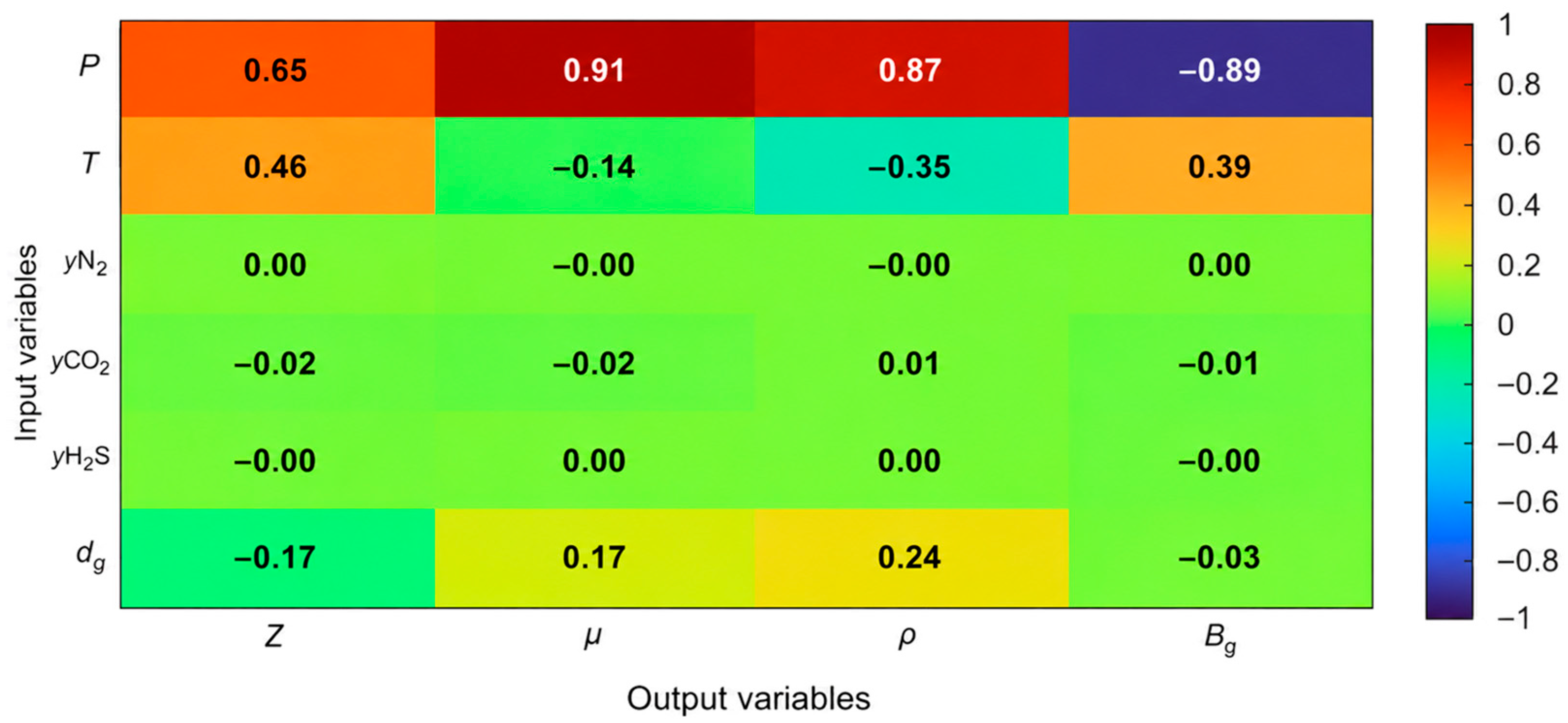
A correlation analysis was conducted using the Spearman correlation coefficient to evaluate the relationships between the input variables and the natural gas output properties considered in this study. This analysis allows the degree of influence of each input variable on the predicted properties to be identified, contributing to a better understanding of the physical behavior of the dataset used in model development.

The Spearman correlation coefficient is a nonparametric statistical measure that evaluates the strength and direction of the monotonic relationship between two variables. The correlation coefficient ranges from −1 to 1, where values close to +1 indicate a strong positive monotonic correlation, values close to −1 indicate a strong negative monotonic correlation, and values close to zero indicate no significant correlation between the analyzed variables.

In this study, the analysis was applied to evaluate the relationship between the input variables, pressure (P), temperature (T), mole fractions of N₂, CO₂, and H₂S, and gas specific gravity (dg), and the model output properties, corresponding to the compressibility factor (Z), gas viscosity (μ), gas density (ρ) and gas formation volume factor (B_g). The correlation matrix was represented as a heatmap, allowing visualization of the degree of association among the analyzed variables.

This analysis also enables verification of the physical consistency of the relationships present in the dataset, as the thermodynamic properties of natural gas exhibit well-established dependencies on pressure, temperature, and non-hydrocarbon composition.

It should be noted that the interpretation of correlation coefficients must consider the sampling ranges adopted for each variable. Components such as N₂ and H₂S exhibit relatively narrow concentration intervals in the present dataset; therefore, low correlation coefficients may partially reflect limited variability rather than the absence of physical influence on the thermophysical properties.

2.4. Artificial Neural Network Architecture

Artificial neural networks (ANNs) consist of computational structures composed of interconnected artificial neurons, whose internal parameters (synaptic weights and biases) are adjusted during the training process. This structure enables the model to learn nonlinear relationships between input and output variables directly from data. The performance of an ANN depends on the definition of key hyperparameters, including the network architecture (e.g., feedforward or recurrent), the number of layers and neurons in each layer, the training algorithm responsible for updating weights and biases, and the activation function used to introduce nonlinearity into the modeling process [26].

In this study, a supervised learning approach was adopted, in which the model is trained using known input–output data pairs. A feedforward Multilayer Perceptron (MLP) artificial neural network was implemented in the MATLAB R2025b (MathWorks Inc., Natick, MA, USA) environment and trained using the error backpropagation algorithm. In the literature, this configuration is commonly referred to as a Backpropagation Neural Network (BPNN).

The developed model was designed to simultaneously estimate four physicochemical properties of natural gas: compressibility factor (Z), gas viscosity (μ), gas density (ρ), and gas formation volume factor (B_g). The selection of a backpropagation-trained MLP was motivated by its ability to model complex nonlinear relationships between input and output variables, and its widespread application in regression and pattern recognition problems in engineering [10].

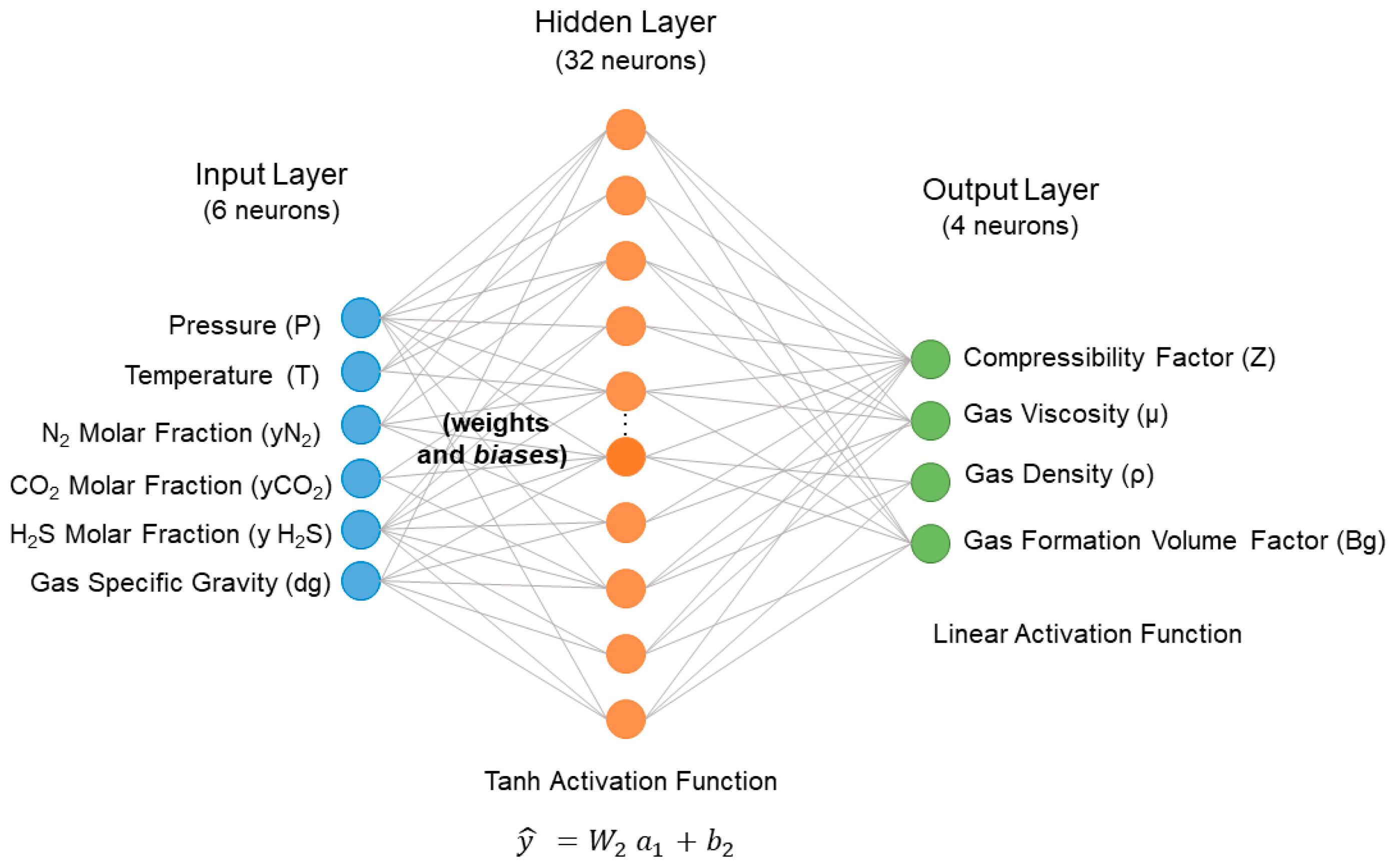
The network comprises six input variables corresponding to the thermodynamic properties of the system: pressure (P), temperature (T), mole fractions of N₂, CO₂, and H₂S, and gas specific gravity (d_g). The output layer consists of four neurons associated with the predicted properties (Z, μ, ρ, and B_g). The number of neurons in the hidden layer was determined based on a model performance analysis, considering different architectural configurations.

To determine the optimal network complexity, architectures with hidden-layer sizes ranging from 10 to 40 neurons were evaluated. The final architecture was selected based on the comparative analysis of the prediction errors obtained for the four target properties, as described in Section 3.2.

The adoption of a single hidden layer was motivated by the Universal Approximation Theorem, which states that feedforward neural networks with nonlinear activation functions can approximate continuous multivariate functions with arbitrary accuracy, provided that a sufficient number of hidden neurons is employed [27,28]. Therefore, a single hidden layer was considered an appropriate architecture for the present regression problem, while the optimal number of hidden neurons was determined empirically through performance evaluation, as discussed in Section 3.2.

Equation (4) shows that the hidden layer uses the hyperbolic tangent activation function:

$$f\left(u\right)=tanh\left(u\right)$$

(4)

The output layer employs a linear activation function, which is suitable for continuous multi-output regression problems.

Mathematically, the model can be described by Equations (5) and (6):

$$a_1=tanh(W_{1}x+b_1)$$

(5)

$$y_{norm}=W_2{a}_1+b_2$$

(6)

where W₁ and W₂ are the weight matrices, and b₁ and b₂ are the bias vectors of the hidden and output layers, respectively.

The properties in the physical scale were obtained by applying the inverse standardization transformation, as defined in Equation (7):

$$y=y_{norm} · {\sigma }_y+{\mathrm{m}}_y$$

(7)

where σ_y and m_y correspond to the standard deviation and mean of the output variables, respectively.

The use of a single neural network to estimate multiple properties enables the joint helps preserve physical self-consistency among the predicted properties. This approach reduces the likelihood of inconsistencies between interrelated thermophysical properties that may arise when independent models are used for each variable, thereby contributing to greater physical coherence in the model predictions.

2.5. Neural Network Training

The neural network was trained using the Levenberg–Marquardt [29] algorithm, which is widely employed in nonlinear regression problems due to its high convergence efficiency [2,12,14]. The learning process was conducted in a supervised manner, using previously known input–output data pairs.

The dataset was divided into three independent subsets: 70% of the data were used for training, 15% for validation, and 15% for testing. The training set was used to adjust the neural network parameters, while the validation set was used to monitor model performance during training and to monitor the model generalization performance during training. The test set was used exclusively to evaluate the model’s generalization capability.

During training, the input and output variables were standardized using the z-score method, as described in Section 2.2, with the aim of improving the numerical stability of the optimization process and preventing the dominance of variables with larger orders of magnitude. The neural network training consisted of minimizing a loss function based on the Mean Squared Error (MSE) between the model predictions and the reference values.

Training was terminated when the predefined maximum number of 1000 epochs was reached. The validation subset was monitored throughout the training process to assess generalization performance. After training the network, the model performance was evaluated by comparing the values predicted by the neural network with the reference values obtained from the thermodynamic correlations used in dataset generation.

2.6. Model Evaluation Metrics

The predictive performance of the proposed model was evaluated using statistical metrics widely employed in regression problems, including Mean Absolute Error (MAE), Mean Squared Error (MSE), Root Mean Squared Error (RMSE), and the coefficient of determination (R²). These metrics were calculated separately for the training, validation, and test sets for the four properties predicted by the model (Z, μ, ρ, and B_g), with the results obtained from the test set used as the primary reference for evaluating the model’s generalization capability.

The Mean Absolute Error (MAE), expressed in Equation (8), represents the average of the absolute differences between the values predicted by the neural network and the reference values, and is given by:

$$MAE={\displaystyle \frac{1}{n}}{\displaystyle {\sum }_{i=1}^n}|y_i-{\widehat{y}}_i|$$

(8)

where y_i represents the reference value of the analyzed property, ${\widehat{y}}_i$ denotes the value estimated by the neural network, and n represents the total number of samples. The MAE provides a direct measure of the average error magnitude and is less sensitive to the presence of outliers.

The Mean Squared Error (MSE), shown in Equation (9), was used as the loss function during neural network training and is defined as:

$$MSE={\displaystyle \frac{1}{n}}{\displaystyle {\sum }_{i=1}^n}(y_i-{\widehat{y}}_i{)}^2$$

(9)

This metric penalizes larger errors more heavily due to the squared term, making it well suited for optimization processes based on least-squares methods, such as the Levenberg–Marquardt algorithm [29].

The Root Mean Squared Error (RMSE), presented in Equation (10), corresponds to the square root of the MSE and has the same unit as the output variable, facilitating the physical interpretation of the prediction error.

$$RMSE=\sqrt{{\displaystyle \frac{1}{n}}{\displaystyle {\sum }_{i=1}^n}(y_i-{\widehat{y}}_i{)}^2}$$

(10)

Lower RMSE values indicate closer agreement between the model predictions and the reference values.

Equation (11) presents how the coefficient of determination (R²) was calculated to evaluate the degree of correlation between the predicted values and the reference values.

$$R^2=1-{\displaystyle \frac{{\displaystyle {\sum }_{i=1}^n}(y_i-{\widehat{y}}_i{)}^2}{{\displaystyle {\sum }_{i=1}^n}(y_i-\overline{y}{)}^2}}$$

(11)

where $\overline{y}$ represents the mean of the reference values. The coefficient R² ranges from 0 to 1, with values close to unity indicating a high degree of agreement between the model predictions and the reference data.

Additionally, a regression analysis between the predicted and reference values was performed using parity plots, allowing a visual assessment of the model’s goodness of fit. The proximity of the data points to the identity line (y = x) was considered indicative of adequate predictive capability.

The combined use of these metrics enables a comprehensive evaluation of model performance. In this way, both the magnitude of errors and the quality of the fit between predicted and reference values can be simultaneously assessed.

In this study, MSE values below 0.01 and RMSE values less than or equal to 0.03 were considered indicative of good predictive performance of the model. These thresholds are consistent with criteria adopted in the literature for regression problems in engineering [11,30].

In addition to the internal training, validation, and test procedures, an independent experimental validation was subsequently performed using literature data not employed during model development. The details and results of this validation are presented in Section 4.4.

2.7. Application to Pressure Drop Calculation

To evaluate the practical applicability of the developed model, the gas compressibility factor (Z) estimated by the neural network was incorporated into pressure drop calculations in natural gas production pipelines using the classical Cullender and Smith [19] method.

The method was applied to real data from seven gas-producing wells reported in the literature, as described in the study by Yusrizal and Santoso [31]. The operational data used include gas production rate, tubing internal diameter, gas specific gravity, well depth, flowing wellhead pressure (P_tf), measured flowing bottom-hole pressure (P_wf), and operating temperatures along the production string.

The method was implemented in the MATLAB environment through a parametric algorithm that allows the definition of the operating conditions for each well. The analyzed wells are assumed to be vertical, and the tubing strings have specific internal diameters and lengths, as presented in

Table 3. Operating Conditions and Well Parameters Used in the Application of the Cullender and Smith [19] Method.

Well	q (MMscfd)	DI (in)	dg	L (ft)	Pwf (psia)	Ptf (psia)	Twf (°F)	Ttf (°F)
01	4.20	1.995	0.746	13,904	2170	1345	278	121
02	7.75	2.992	0.718	10,730	2518	1812	207	110
03	3.11	1.995	0.755	11,682	1942	1383	240	121
04	12.85	2.992	0.700	12,464	3114	2235	257	128
05	3.50	1.995	0.700	12,523	1838	1240	246	128
06	2.61	2.992	0.780	12,716	2061	1455	260	121
07	2.91	2.992	0.693	12,854	2347	1786	276	121

Source: Adapted from Yusrizal and Santoso [31]. Note: q = gas flow rate; DI = tubing internal diameter; d_g = gas specific gravity; L = tubing length; P_wf = flowing bottom-hole pressure; P_tf = flowing wellhead pressure; T_wf and T_tf = bottom-hole and wellhead temperatures, respectively.

, along with the pressure, temperature, and flow rate conditions used in the calculations.

It should be noted that Well 06 presents a gas specific gravity of 0.78, whereas the training dataset was developed using values between 0.50 and 0.70. Therefore, this case represents an extrapolation of approximately 11.4% beyond the upper training limit. Although the proposed BPNN produced physically consistent predictions for this condition, extrapolative results should be interpreted with additional caution because neural networks generally exhibit greater reliability within the interpolation domain.

All assumptions and parameters of the original Cullender and Smith [19] hydraulic formulation were kept unchanged during the application of the method. The only modification introduced consisted of replacing the conventional procedure for obtaining the gas compressibility factor—traditionally determined from the Standing and Katz [32] chart—with the values estimated by the BPNN model developed in this study.

The pressure drop in the tubing was calculated based on the estimation of the flowing bottom-hole pressure (P_wf) obtained using the Cullender and Smith [19] method. The calculated pressure loss in the tubing corresponds to the difference between the calculated flowing bottom-hole pressure and the flowing wellhead pressure (P_tf). Similarly, the field-measured pressure drop was obtained from the difference between the measured flowing bottom-hole pressure and the flowing wellhead pressure recorded under operating conditions Yusrizal and Santoso [31].

This step enabled the evaluation of the physical consistency and practical applicability of the natural gas thermophysical property prediction model. In particular, it was assessed whether the compressibility factor estimated by the neural network is capable of producing consistent results when incorporated into a classical hydraulic model widely used in gas production engineering.

3. Results

3.1. Spearman Correlation Analysis

Spearman correlation was computed to investigate the monotonic relationships between the input variables and the output properties of the dataset prior to neural network training. This analysis enables the identification of the degree of association between variables and provides a preliminary indication of the prediction difficulty for each property, as outputs with low correlation to the input variables tend to exhibit higher modeling complexity. In addition, the analysis contributes to the interpretation of the physical behavior of the data.

Figure 1 presents the Spearman correlation matrix between the input variables, pressure (P), temperature (T), mole fractions of N₂, CO₂, and H₂S, and gas specific gravity (d_g), and the output properties considered in this study, namely the compressibility factor (Z), gas viscosity (μ), gas density (ρ), and gas formation volume factor (B_g). In this analysis, the Spearman correlation coefficient (r_s) ranges from −1 to 1 and indicates the strength and direction of the monotonic association between the analyzed variables.

The results indicate that pressure (P) is the primary controlling parameter of the system. A strong positive monotonic correlation is observed between pressure and gas viscosity (r_s = 0.91) and between pressure and gas density (r_s = 0.87), as well as a strong negative monotonic correlation between pressure and the gas formation volume factor (r_s = −0.89).

Temperature (T) exhibits a secondary influence on the analyzed properties. A moderate negative correlation with gas density (r_s = −0.35) and a positive correlation with the gas formation volume factor (r_s = 0.39) are observed. The correlation between temperature and the compressibility factor (Z) shows a moderate magnitude (r_s = 0.46).

The composition variables (yN₂, yCO₂, and yH₂S) exhibit correlation coefficients close to zero in the considered dataset. Similarly, gas specific gravity (d_g) exhibited weak correlations with the analyzed properties (|r_s| < 0.25).

Overall, the observed correlation structure confirms the physical consistency of the dataset and highlights the predominance of pressure effects on the thermophysical properties of natural gas.

3.2. Network Architecture Selection

The definition of the number of neurons in the hidden layer represents one of the main hyperparameters in the development of artificial neural networks, directly influencing the model’s ability to capture nonlinear relationships between input and output variables.

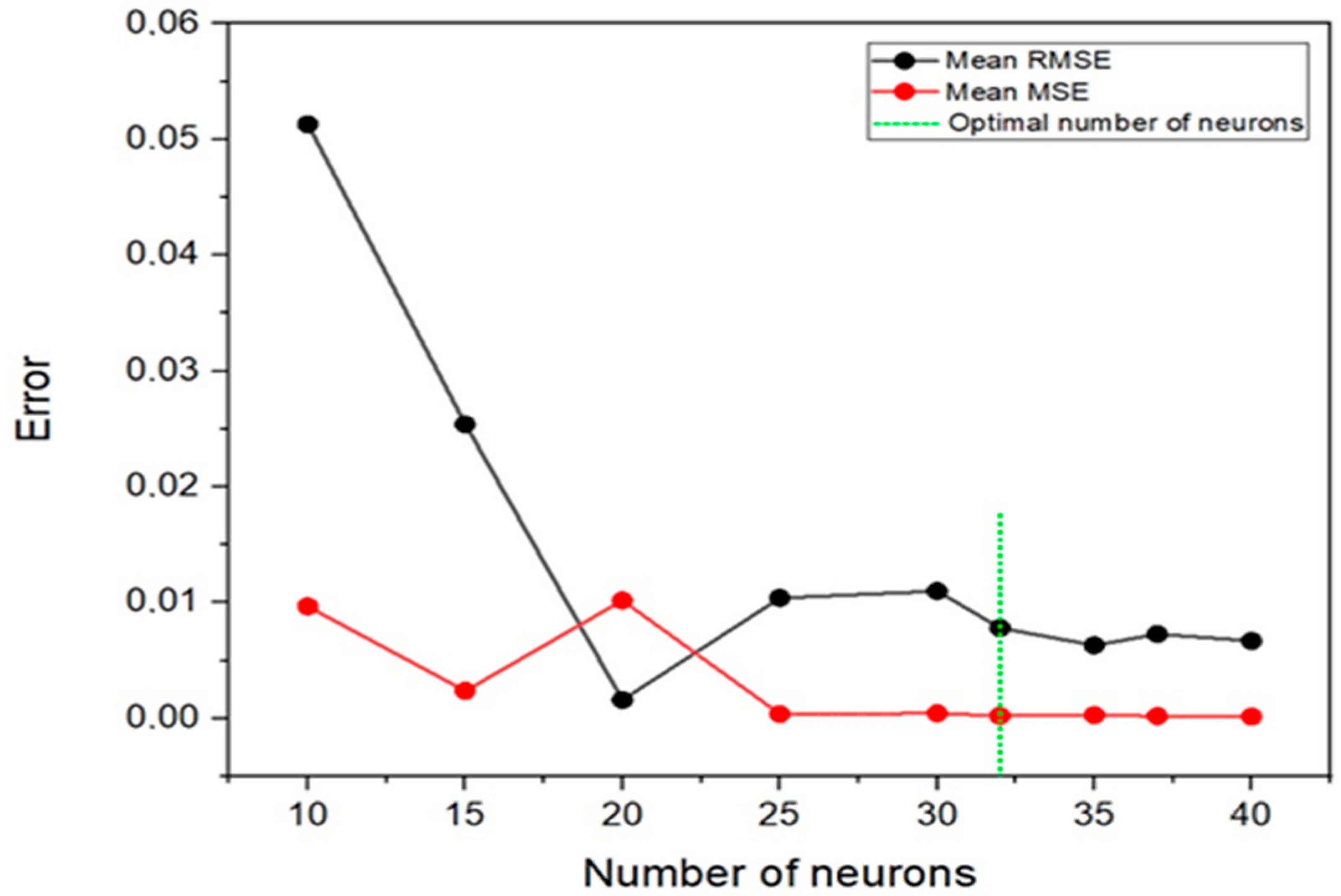
To evaluate the influence of this parameter, neural networks with different numbers of neurons in the hidden layer were trained, ranging from 10 to 40. For each configuration, a global average error was calculated, obtained from the arithmetic mean of the RMSE and MSE values for the four estimated properties (Z, μ, ρ, and B_g).

Figure 2 presents the variation in the global average errors (RMSE and MSE) as a function of the number of neurons in the hidden layer. A significant reduction in error is observed for architectures with up to approximately 32 neurons. Beyond this point, the reduction in error becomes marginal.

Although the Universal Approximation Theorem supports the use of a single hidden layer, it does not prescribe the optimal number of neurons for a specific application. Therefore, the hidden-layer size was determined empirically through the evaluation of multiple network configurations. The architecture containing 32 hidden neurons produced the lowest global average prediction error, calculated from the average RMSE and MSE values of the four target properties (Z, μ, ρ, and B_g), while maintaining stable training behavior. Consequently, this configuration was selected as the final model architecture.

Thus, the architecture with 32 neurons was selected as it represents an appropriate trade-off between predictive accuracy and model complexity. For this configuration, average RMSE and MSE values of approximately 7.82 × 10⁻³ and 2.26 × 10⁻⁴, respectively, were obtained.

Figure 3 presents the final neural network architecture adopted in this study (6–32–4), consisting of six input neurons, one hidden layer with 32 neurons, and four output neurons.

This configuration exhibited the best overall performance among the evaluated architectures while maintaining stability during the training process.

3.3. Network Training Performance

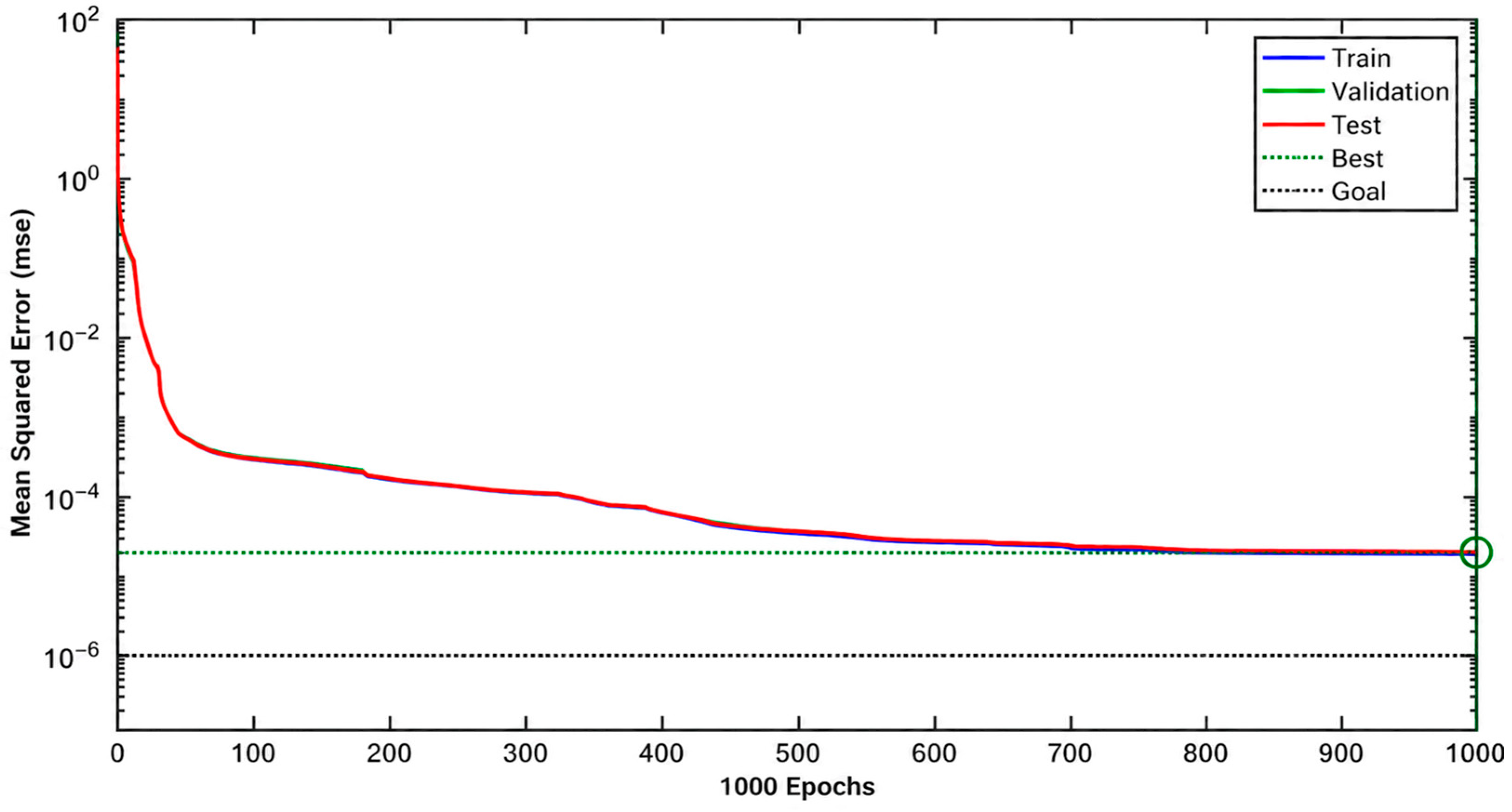
Figure 4 presents the evolution of the Mean Squared Error (MSE) over the training epochs of the BPNN artificial neural network, using the Levenberg–Marquardt [29] optimization algorithm. The architecture adopted for the model was 6–32–4, consisting of six neurons in the input layer, one hidden layer with 32 neurons, and four neurons in the output layer, corresponding to the predicted thermophysical properties (Z, μ, ρ, and B_g).

A sharp reduction in error is observed during the initial training epochs. After approximately 100 epochs, the rate of error reduction becomes more gradual.

The best validation performance was achieved at epoch 1000, with an MSE value of 2.1262 × 10⁻⁵, corresponding to the maximum number of training epochs specified. Therefore, training was terminated by the predefined epoch limit rather than by a validation-based early stopping criterion. Nevertheless, the training, validation, and test curves remained closely overlapped throughout the training process, indicating stable convergence and the absence of significant overfitting.

The reduction of the MSE to the order of 10⁻⁵ indicates good accuracy in the model training process. Moreover, the smooth behavior of the error curves on a logarithmic scale confirms the stability of the training procedure.

To ensure reproducibility of the proposed model, the weight matrices and bias vectors associated with the trained neural network are provided in the Supplementary Materials of this work. These parameters correspond to the matrices W₁ and W₂, and the bias vectors b₁ and b₂ defined for the final network architecture.

3.4. Comparative Performance Analysis

Table 4. Statistical performance metrics of the BPNN model for the training and test sets in predicting the properties Z, μ, ρ, and B_g.

Property	Dataset	RMSE	MSE	MAE	R2
Z	training	0.0005356	2.87 × 10−7	0.0003770	1.00
	testing	0.0005565	3.10 × 10−7	0.0003900	1.00
μ	training	0.0000322	1.07 × 10−9	0.0000227	1.00
	testing	0.0000324	1.05 × 10−9	0.0000229	1.00
ρ	training	0.0290160	8.42 × 10−4	0.0197470	1.00
	testing	0.0300750	9.05 × 10−4	0.0203450	1.00
Bg	training	0.0006389	4.08 × 10−7	0.0003879	1.00
	testing	0.0006329	4.01 × 10−7	0.0003868	1.00

presents the performance of the BPNN model for the training and test sets using the statistical metrics RMSE, MSE, MAE, and R² for the four predicted properties (Z, μ, ρ, and B_g).

A high level of consistency is observed in the results, evidenced by the small difference between the errors obtained for the training and test sets.

For the compressibility factor (Z), the RMSE ranges from 5.36 × 10⁻⁴ in training to 5.56 × 10⁻⁴ in the test set. Similar results are observed for gas viscosity (μ), for which RMSE values remain on the order of 10⁻⁵ for both training and testing.

Gas density (ρ) exhibits higher absolute error values compared to the other properties. Even in this case, the difference between training (RMSE = 0.0290) and testing (RMSE = 0.0301) errors remains small.

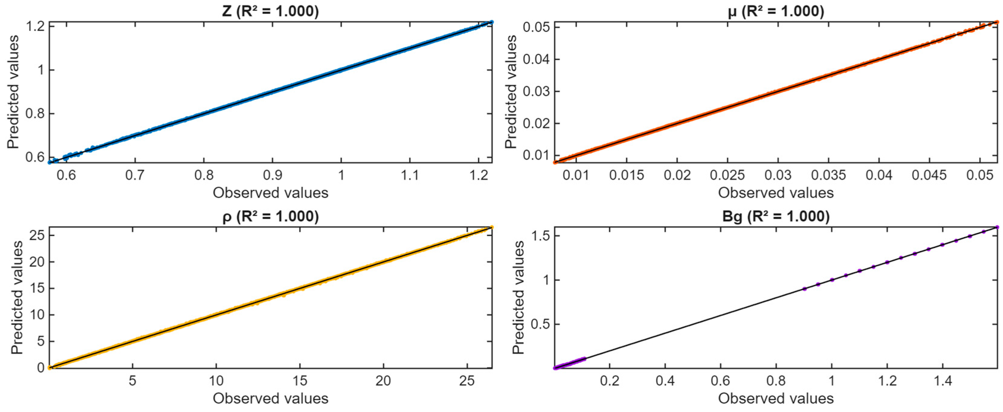
For the gas formation volume factor (B_g), RMSE values remain on the order of 10⁻⁴ for both the training and test sets. Overall, the combined analysis of the RMSE, MSE, MAE, and R² metrics indicates a high degree of agreement between the predicted and reference values.

Figure 5 presents the parity plots between the values estimated by the neural network and the reference values for the properties Z, μ, ρ, and B_g.

It is observed that the data points remain concentrated near the identity line (y = x) for all analyzed properties.

3.5. Validation Against Literature Data and Applicability in Pressure Drop Calculation

The applicability of the proposed model was evaluated through its integration into pressure drop calculations in pipelines using the Cullender and Smith [19] method.

To evaluate the physical consistency and practical applicability of the developed model, the compressibility factor (Z) estimated by the MLP (BPNN) neural network was directly incorporated into the hydraulic model, while the original formulation of the method was kept unchanged.

Validation was performed using data from seven producing wells reported by Yusrizal and Santoso [31], including bottom-hole pressure measurements and operating conditions.

The field application dataset provided wellhead pressure, bottom-hole flowing pressure, temperature, flow conditions, and gas specific gravity data. However, detailed gas-composition information was not reported in the original reference. Consequently, the mole fractions of N₂, CO₂, and H₂S required as inputs to the proposed BPNN were assumed to be zero for all evaluated wells. This assumption should be considered when interpreting the results, since the actual gas compositions were unavailable.

It should also be noted that the gas specific gravity reported for the evaluated wells (d_g = 0.78) lies slightly above the training range adopted during model development (0.5 ≤ d_g ≤ 0.7). Therefore, the field application involves a limited extrapolation beyond the original training domain. Although satisfactory agreement was obtained, prediction uncertainty may increase under extrapolation conditions, and the reported results should be interpreted accordingly.

Table 5. Comparison between measured bottom-hole pressure and predicted values using Cullender and Smith (C&S) and the proposed BPNN-based approach, along with their respective mean percentage errors (MPE).

Well Name	Measured Pwf (psia)	Pwf C&S (psia)	Pwf BPNN (psia)	Error C&S (%)	Error BPNN (%)
01	2170	2318	2308	6.82	6.35
02	2518	2507	2510	0.44	0.31
03	1942	2072	2071	6.69	6.64
04	3114	3243	3248	4.14	4.30
05	1838	1925	1927	4.73	4.84
06	2061	2080	2077	0.92	0.80
07	2347	2419	2422	3.07	3.21
Mean percentage error				3.83	3.78

Source: Adapted from Yusrizal and Santoso [31].

presents a comparison between the measured bottom-hole flowing pressures and the values predicted using both the original Cullender and Smith method and the proposed BPNN-based approach. The corresponding prediction errors are also reported to assess the impact of incorporating the neural-network-estimated compressibility factor into the hydraulic calculations.

Additionally, the assumed value of yCO₂ = 0 lies outside the compositional range represented in the training dataset (14–25 mol% CO₂). Consequently, the field application also involves compositional extrapolation, which constitutes an additional source of uncertainty. In the absence of reported compositional data for the evaluated wells, the results should be interpreted with appropriate caution.

The results indicate that the proposed approach adequately reproduces bottom-hole pressure values, with a mean percentage error of 3.78%, comparable to that obtained with the classical method (3.83%).

Table 6. Comparison between measured and calculated pressure drops and associated prediction errors.

Measured ΔP (psi)	Calculated ΔP C&S (psi)	Erro ΔP C&S (%)	Calculated ΔP BPNN (psi)	Erro ΔP BPNN (%)
825	973	17.94	963	16.73
706	695	1.56	698	1.13
559	689	23.26	688	23.08
879	1008	14.68	1013	15.24
598	685	14.55	687	14.88
606	625	3.14	622	2.64
561	633	12.83	636	13.37
Average	-	12.56	-	12.44

presents the comparison between measured and calculated pressure drop values using both approaches.

It is observed that the pressure drop values calculated by both approaches remain close for all analyzed wells.

Although the average relative errors calculated using the bottom-hole flowing pressure (P_wf) were below 4% for both methods, this metric may provide a relatively optimistic assessment because the reference pressure appears in the denominator and is substantially larger than the corresponding pressure drop along the tubing. To provide a more conservative evaluation, the pressure-drop error was also calculated using:

$${Erro}_{\Delta P} = {\displaystyle \frac{{\Delta P}_{calc} - {\Delta P}_{meas}}{{\Delta P}_{meas} · 100}}$$

(12)

where ΔP represents the pressure drop between the wellhead and bottom-hole conditions. Based on the values presented in Table 6, the average pressure-drop errors were 12.56% for the Cullender and Smith method and 12.44% for the proposed BPNN approach. These results indicate that both methods exhibit comparable performance when evaluated using pressure-drop criteria.

Although the ΔP-based errors are higher than those obtained using the P_wf metric, the proposed BPNN-based approach produced virtually the same pressure-drop accuracy as the original Cullender and Smith formulation (12.44% versus 12.56%). Therefore, the observed uncertainty is primarily associated with the hydraulic model itself rather than with the neural-network estimation of the compressibility factor. From an engineering perspective, the results demonstrate that the proposed BPNN can replace the iterative compressibility-factor calculation without introducing any significant degradation in hydraulic performance.

Overall, the results demonstrate that the BPNN model developed for estimating natural gas thermophysical properties can be integrated into classical hydraulic models without loss of accuracy in engineering calculations.

4. Discussion

4.1. Interpretation of Correlation Patterns and Nonlinear Relationships

The observed correlation structure confirms the physical consistency of the dataset and highlights the predominance of pressure effects on the thermophysical properties of natural gas. The increase in pressure promotes greater molecular compaction, increasing both fluid density and viscosity, while simultaneously reducing the gas specific volume, which is reflected in a decrease in the gas formation volume factor (B_g).

The behavior observed for temperature is associated with the thermal expansion effect of the fluid. In addition, the moderate correlation between temperature and the compressibility factor (Z) indicates that thermal effects contribute to deviations from ideal gas behavior, although their influence is lower than that exerted by pressure under the analyzed conditions.

It is important to note, however, that Spearman correlation assesses only monotonic associations between variables and does not capture more complex nonlinear interactions. Some variables, such as the mole fractions of N₂, CO₂, and H₂S, exhibit low correlation coefficients, indicating a weak monotonic association with the analyzed properties. However, this result does not imply the absence of dependence between variables and may reflect the presence of more complex nonlinear relationships.

It should be noted that the interpretation of the correlation coefficients must consider the sampling ranges adopted for each input variable. In particular, N₂ and H₂S were represented within relatively narrow concentration intervals, resulting in limited statistical variability. Consequently, the low correlation coefficients observed for these components may partially reflect the restricted sampling range rather than the absence of physical influence on the thermophysical properties. Therefore, the correlation analysis should be interpreted primarily as a description of the behavior within the investigated domain rather than a definitive measure of variable importance.

Therefore, the observed low correlations do not necessarily imply the absence of dependence between variables. Instead, they may result from a combination of limited statistical variability and nonlinear relationships that cannot be fully captured by a monotonic correlation metric.

In this context, the use of artificial neural network–based models is appropriate, as these models are capable of capturing nonlinear relationships between input and output variables.

4.2. Influence of Network Architecture on Predictive Performance

The definition of the number of neurons in the hidden layer directly influences the model’s ability to capture nonlinear relationships between input and output variables. An insufficient number of neurons may result in underfitting, limiting the network’s ability to adequately represent the complexity of the system, whereas an excessive number may lead to overfitting, compromising the model’s generalization capability.

The reduction in error observed up to approximately 32 neurons indicates an improvement in the model’s ability to represent nonlinear relationships among the variables. Beyond this point, the reduction in error becomes marginal, indicating a saturation trend in learning capacity. This behavior is consistent with an increase in model complexity without significant performance gains and may even compromise the model’s generalization capability.

The rapid convergence observed during training highlights the efficiency of the Levenberg–Marquardt algorithm. This method combines features of gradient descent and the Gauss–Newton approach, enabling efficient adjustment of synaptic weights and accelerating the minimization of the cost function.

The absence of significant divergence between training, validation, and testing curves indicates good generalization capability and the absence of overfitting, suggesting that the adopted architecture (6–32–4) is suitable for representing the complexity of the relationships between the input variables and the system’s output properties.

4.3. Comparison with Previous Studies

The results obtained demonstrate excellent predictive capability for all evaluated thermophysical properties. However, the interpretation of these performance metrics requires consideration of the nature of the dataset employed in this study. The target properties used for network training (Z, μ, ρ, and B_g) were generated from well-established thermodynamic and empirical correlations, including Hall–Yarborough and Carr et al., whereas the compositional domain was defined using representative concentrations of non-hydrocarbon components (N₂, CO₂, and H₂S) observed in Brazilian pre-salt reservoirs.

Several previous studies have reported artificial neural network models for predicting natural gas properties. Nevertheless, direct quantitative comparisons of RMSE and R² values should be interpreted with caution because many of these studies were developed or validated using experimental datasets, which contain measurement uncertainty and different error structures. Therefore, differences in data origin, operating conditions, and input-variable distributions may substantially influence the reported performance metrics.

For gas density (ρ), higher absolute error values were observed compared with the other predicted properties. This behavior is mainly associated with the broader numerical range of density values in the dataset, extending from values close to zero up to approximately 26 lb/ft³. Although some studies report lower RMSE values, direct comparisons remain limited due to differences in dataset characteristics and validation procedures.

For the gas formation volume factor (B_g), the scarcity of published machine-learning studies reporting detailed performance metrics limits comprehensive benchmarking. Nevertheless, the results demonstrate that the proposed BPNN accurately reproduces the behavior predicted by the adopted thermodynamic correlations throughout the investigated operating range.

An important distinction of the proposed approach is the simultaneous estimation of multiple thermophysical properties within a single neural network. This strategy increases the complexity of the regression problem when compared with single-output models, while contributing to the preservation of physical self-consistency among the predicted properties. In this framework, the network learns a common representation of the thermodynamic state of the gas, allowing the joint prediction of Z, μ, ρ, and B_g from the same set of input variables.

The high predictive performance of the model can be attributed to three main factors: the broad coverage of the operational variable space represented in the dataset; the multi-output architecture adopted for simultaneous property estimation; and the use of the Levenberg–Marquardt algorithm [29], which promotes efficient parameter adjustment in nonlinear regression problems. Consequently, the excellent predictive metrics obtained in this study should be interpreted primarily as evidence of the BPNN’s ability to reproduce the underlying thermodynamic correlations with high fidelity within a physically representative operational domain, while providing an explicit, non-iterative, and computationally efficient surrogate representation of the adopted correlations.

4.4. Independent Validation Using Experimental Data

To provide an independent assessment of the proposed model, additional validation was performed using experimental compressibility-factor data reported by Buxton and Campbell [33] or CO₂-rich natural-gas mixtures. These data were not used during model development or training.

Since the original experimental mixture presented a gas specific gravity slightly above the training range of the proposed BPNN, the validation was conducted using the maximum gas-specific-gravity value included in the training domain (d_g = 0.70), thereby avoiding extrapolation during the primary validation procedure.

Table 7. Comparison between experimental compressibility-factor data reported by Buxton and Campbell [33] and the corresponding BPNN predictions within the training domain (d_g = 0.70).

P (psia)	T (°F)	Zexp	ZBPNN (dg = 0.70)	Error (%)
1026	100	0.865	0.8735	0.97
1526	100	0.814	0.8238	1.18
2026	100	0.778	0.7891	1.41
2526	130	0.814	0.8155	0.18
3026	130	0.82	0.8167	0.40
3526	130	0.839	0.831	0.96
4026	130	0.867	0.8552	1.38
4526	160	0.924	0.9092	1.63
5026	160	0.956	0.9403	1.67
6026	160	1.034	1.011	2.27
7026	160	1.115	1.090	2.34

compares the experimental compressibility-factor values with the corresponding BPNN predictions.

The results indicate good agreement between the experimental measurements and the corresponding BPNN predictions over the entire pressure range investigated. Most relative errors remained below 2%, with the maximum deviation being approximately 2.34%.

The model achieved an Average Absolute Relative Deviation (AARD) of 1.31% and an RMSE of 0.0255, indicating excellent agreement with the experimental measurements. A summary of the statistical performance metrics obtained for both the validation and sensitivity-analysis cases is presented in

Table 8. Summary of statistical performance metrics obtained for the independent experimental validation.

Validation Case	AARD (%)	RMSE
Buxton and Campbell experimental dataset (dg = 0.70)	1.31	0.0255
Sensitivity analysis (dg = 0.78)	3.94	0.0340

.

These results provide independent experimental support for the proposed methodology and complement the validation performed using thermodynamic correlations and hydraulic calculations. As expected, the prediction error increased when the actual gas specific gravity of the experimental mixture (d_g = 0.78) was employed, since this value lies slightly outside the training range adopted for the BPNN (0.5–0.7). Under this extrapolation condition, the AARD increased from 1.31% to 3.94%. Nevertheless, the model maintained satisfactory agreement with the experimental measurements, indicating reasonable robustness under limited extrapolation conditions.

A preliminary assessment of model behavior near the upper boundary of the gas-specific-gravity training range also indicated a modest increase in prediction error, consistent with the expected reduction in reliability of data-driven models as predictions approach extrapolation conditions.

4.5. Engineering Applicability and Practical Implications

The proposed approach establishes a hybrid modeling framework, in which thermophysical properties are estimated using machine learning and incorporated into classical flow equations.

Although several studies have explored the use of neural networks for predicting natural gas properties, the direct integration of these predictions into classical hydraulic models remains underexplored in the literature. To the best of the authors’ knowledge, no studies have been identified that use multi-output neural networks to simultaneously estimate thermophysical properties and directly integrate them into the Cullender and Smith [19] method for pressure drop calculation.

In this context, the proposed approach offers relevant advantages. First, the use of a single multi-output model enables the simultaneous estimation of multiple properties while preserving the physical relationships among them. Moreover, this strategy reduces implementation complexity in practical applications by eliminating the need to use different correlations or independent models for each property within simulation codes.

The results indicate that replacing the compressibility factor obtained from the Standing and Katz [32] chart with the BPNN-estimated values does not compromise the accuracy of the hydraulic calculations. In addition, replacing the chart-based procedure with a neural network formulation enhances flexibility for implementation in computational routines and flow simulators.

These results indicate that the BPNN model preserves the physical behavior embedded in the original hydraulic method, maintaining consistency between thermodynamic properties and the flow equations used in pressure drop calculations.

4.6. Limitations and Future Perspectives

It is important to note that the range of gas specific gravity considered during model training (0.5 ≤ d_g ≤ 0.7) is lower than the values used in the application stage, which reach up to d_g = 0.78, characterizing an extrapolation condition.

In data-driven models such as artificial neural networks, generalization is generally more reliable within the training domain, while extrapolation is associated with greater uncertainty [10,27,34]. Recent studies also indicate that machine learning models tend to perform better under interpolation conditions than in extrapolative regimes, with potential loss of accuracy outside the training data range [10].

Nevertheless, the results obtained indicate that the model maintains consistent performance under these conditions, suggesting good robustness. However, caution is recommended when applying the model outside the training range.

Overall, the developed model demonstrates potential for application in flow simulations, reservoir modeling, and the development of computational tools in the oil and gas industry. Additionally, the simultaneous prediction of four thermophysical properties (Z, μ, ρ, and B_g) facilitates integration into computational simulation frameworks, reducing implementation complexity and ensuring consistency among the variables used in engineering calculations.

4.7. Limitations and Scope of Applicability

The proposed BPNN was developed as a surrogate model of established thermodynamic correlations rather than as a direct replacement for laboratory PVT measurements. Consequently, the excellent predictive performance reported in this study should be interpreted primarily as the ability of the neural network to reproduce the behavior of the underlying correlations within the investigated domain.

Although the compositional ranges were defined using representative field compositions from Brazilian pre-salt reservoirs, the target properties were generated from established engineering correlations. Therefore, additional validation using independent laboratory measurements and fully characterized field datasets is recommended before extending the proposed approach to broader real-gas applications.

The application example included one case with a gas specific gravity value slightly above the upper training limit. Specifically, the value of 0.78 represents an extrapolation of approximately 11.4% beyond the maximum value used during model development (0.70). Although satisfactory agreement was obtained in this case, extrapolative predictions inherently involve greater uncertainty than interpolation scenarios. Consequently, the proposed model is recommended primarily for applications within the ranges represented in the training dataset, while predictions outside these limits should be interpreted with caution.

5. Conclusions

This study presented the development and validation of a Backpropagation Neural Network (BPNN) model for the simultaneous estimation of four thermophysical properties of natural gas: compressibility factor (Z), viscosity (μ), density (ρ), and gas formation volume factor (B_g). Unlike most studies available in the literature, which predict these properties independently, the proposed model employs a single multi-output neural architecture (6–32–4), enabling integrated estimation of these variables while preserving the physical consistency among interdependent thermodynamic properties.

The model was trained using a dataset composed of 58,165 points, generated from well-established thermodynamic correlations, and optimized using the Levenberg–Marquardt [29] algorithm. The results demonstrated high predictive performance, with coefficients of determination close to unity and RMSE values of 5.56 × 10⁻⁴, 3.24 × 10⁻⁵, 3.01 × 10⁻², and 6.33 × 10⁻⁴ for Z, μ, ρ, and B_g, respectively, corresponding to MSE values of 3.10 × 10⁻⁷, 1.05 × 10⁻⁹, 9.05 × 10⁻⁴, and 4.01 × 10⁻⁷.

For the compressibility factor and gas viscosity, the obtained errors are lower than those reported in previous neural network–based studies, highlighting the advancement of the proposed model in terms of predictive accuracy. For gas density, the absolute error values are higher compared to the other properties, which is associated with the wider variation range of this variable in the dataset, while still maintaining consistent performance across the entire analyzed range. Furthermore, the estimation of the gas formation volume factor (B_g), which remains relatively underexplored in the literature, highlights the contribution of the present study. The close agreement between the errors obtained for the training and test sets highlights the advancement of the proposed model in terms of predictive accuracy, particularly considering the adopted multi-output approach.

The practical applicability of the model was evaluated through its integration into pressure drop calculations in pipelines using the classical Cullender and Smith [19] method. Replacing the compressibility factor obtained from the Standing and Katz [32] chart with values predicted by the neural network resulted in a mean percentage error of 3.78%, which is very close to that obtained with the classical method (3.83%).

This result demonstrates that the use of the BPNN does not compromise the hydraulic consistency of the original formulation. It is noteworthy that the integration of the machine learning model with a classical hydraulic model establishes a hybrid modeling framework capable of replacing traditional procedures based on charts or empirical correlations, while preserving the physical consistency of engineering calculations. This approach expands the model’s potential application in flow simulators and computational systems used in gas production and transportation engineering.

As a direction for future work, it is recommended to expand the model by incorporating experimental data to enhance the representativeness of the considered operating conditions. Additionally, the properties predicted by the model, including the gas formation volume factor (B_g), which remains relatively underexplored in machine learning–based studies, can be integrated into different flow and simulation models, contributing to the development of more robust, accurate, and computationally efficient hybrid frameworks in the oil and gas industry.

6. Patents

A computer program registration application associated with the computational methodology developed in this study has been submitted to the Brazilian National Institute of Industrial Property (INPI) and is currently under evaluation. A full code implementation will be made available upon reasonable request to the corresponding author.