Enhancing Construction Simulation Optimization Performance Through Variance Reduction Techniques

Abstract

Simulation optimization has been used to analyze construction operations and support planning decisions under uncertainty. It enables the identification of effective planning strategies throughout a project’s lifecycle. However, the use of stochastic simulation to evaluate alternative strategies results in higher computational demands and the generation of inferior solutions within the resulting optimal solutions. This study examines the feasibility of overcoming these issues by implementing variance reduction techniques into a discrete-event simulation optimization framework. Three variance reduction techniques are evaluated in a case study: Common Random Numbers, Antithetic Variates, and a combined application of both. While these techniques are well established in simulation, their impact on the optimization performance of construction problems has not been fully explored. The results show that VRT not only reduces the computational effort required to evaluate planning strategies but also provides better planning strategies. Among the evaluated techniques, the combined approach demonstrates the best improvements. Overall, the study highlights that variance reduction techniques can make simulation optimization frameworks more practical and reliable for complex construction projects.

1. Introduction

The construction industry is a critical sector of a country’s economy, delivering infrastructure, buildings, and essential services that support societal development and economic growth. Infrastructure construction projects, such as bridges and transportation systems, require numerous decision-making under significant uncertainty [1]. During the planning and execution phases, the management team’s decisions have a substantial impact on the project’s objectives, influencing cost, duration, resource utilization, and customer satisfaction. As a result, improving the decision-making process for construction projects is a key priority for both researchers and practitioners [1,2,3,4]. As part of project planning, the team should decide, among other things, on construction methods, the number of labor crews and equipment, and scheduling policies to meet the project objectives. These decisions involve complex trade-offs between competing objectives, such as minimizing project duration while controlling cost. This is a classical construction optimization problem that is usually referred to as Time-Cost Trade-off (TCT) [5,6]. In practice, this problem is most often solved using the management team’s experience [4]. In the realm of construction research, researchers have proposed several methods, such as integer programming and metaheuristics algorithms, to solve this problem [5,6].

Estimating the duration and cost of infrastructure projects is not straightforward due to their complex nature and inherent uncertainty. Many researchers have used computer simulations, particularly stochastic discrete-event simulation (DES), to analyze construction operations and estimate project duration and cost [7,8]. DES is a powerful tool used to estimate the performance of a system with a particular set of decision variables [9]. This is done by creating a virtual model that mimics the behavior of a real-world system over time [10]. DES has been used in many fields, such as healthcare [11], manufacturing industry [12], supply chain [13], aviation industry [14], and construction [15]. By representing construction operations as sequences of events over time, one can evaluate alternative planning strategies before implementation. As a result, the integration of simulation and optimization methods has emerged as a powerful framework for solving optimization problems [16,17,18]. This integration is known as simulation optimization or simulation-based optimization. Within this framework, the optimization algorithm generates different planning strategies and selects the optimal one, while the DES calculates the project duration and cost for each strategy.

When stochastic DES is used, a single simulation run is insufficient to obtain an accurate estimate of the project duration and cost. Therefore, multiple simulation runs, or replications, are required to obtain a reliable estimate of the project duration and cost. The larger the number of simulation replications, the longer it takes to evaluate a strategy [19]. As a result, DES optimization can become computationally demanding, particularly for large-scale problems with many decision variables [20]. Replanning during the execution phase can occur for several reasons, and for DES optimization to be useful, it must be efficient and effective in finding the optimal planning strategy. The efficiency of stochastic DES optimization is influenced by two primary factors: (1) the number of solutions examined and (2) the number of simulation replications conducted for each candidate [19]. As a result, a trade-off between the accuracy of estimating the objective functions and the ability to find optimal solutions is usually made. This compromise can ultimately lead to suboptimal solutions and, consequently, flawed decision-making [21,22]. To avoid this, an accurate estimate of the objective functions should be obtained with fewer simulation replications [23].

Variance reduction techniques (VRTs) have the potential to enhance the statistical output of a simulation model through reducing the estimator variance, thereby yielding more precise output measures for a given computational effort [24]. As a result, these techniques reduce the required number of replications to obtain a reliable estimate of a system [10,25]. VRTs have been extensively studied in simulation literature [10,24]. In construction research, VRTs have been applied in a few studies. AbouRizk et al. [26] employed Common Random Numbers (CRNs) to reduce the required number of simulation replications when comparing two alternative earthmoving operation strategies. Similarly, Ioannou and Martínez [27] applied CRNs to evaluate and compare two rock tunneling construction methods, requiring fewer simulation replications for a reliable comparison. These studies have primarily focused on using these techniques to reduce the variance in simulation outputs when comparing predefined planning strategies. The application of VRTs in large construction optimization problems with noisy objective functions remains very limited. In contrast, their influence on the overall performance of optimization algorithms, especially in terms of quality and optimality, is relatively unexplored. This is critical, as stochastic objective functions directly affect the optimization algorithm’s ability to converge, which would result in sub-optimal solutions [21,28].

The primary aim of this study is to investigate how VRTs, specifically CRNs, Antithetic Variates (AVs), and their combined application, influence both efficiency and performance of a DES-optimization framework for construction operations. This study examines the influence on the behavior and outcomes of the optimization process, including the quality and optimality of the generated solutions. This thereby provides insight into their role in enhancing decision-making in construction research and practice. In this paper, the focus is on large multiobjective optimization problems where metaheuristic optimization methods are coupled with stochastic DES. These types of problems can limit the reliability and practicality of simulation optimization as a decision-making tool. Consequently, the following research questions are addressed: (1) What computational time savings are achieved by this application? (2) How do the quality and optimality of the solutions generated using the implemented VRT compare to those generated using independent replications? (3) How do the evaluated VRTs compare to each other under different random-number stream management methods?

The remainder of the manuscript provides a brief literature review in Section 2. The framework and developed algorithms are explained in Section 3. Section 4 applies the framework to a case study and discusses the outcomes in Section 5, and finally, a conclusion of this study is included in Section 6.

2. Background and Related Work

2.1. Variance Reduction Techniques

VRTs are a set of techniques that were developed to improve the statistical efficiency of simulation models. Their aim is to reduce the variance of simulation outcomes while using fewer replications [10,24]. As a result, they allow practitioners to save time on simulating a model without compromising the accuracy of simulation outcomes. This reduction can be achieved by inducing correlations between the simulation replications. Among the various VRTs, CRN and AV are the most used and applicable to this study [10,24,29,30,31,32,33].

CRN is used to compare how a simulation model’s outcomes change under differing input conditions [29]. For example, it can be used to calculate project duration and cost using different decision variables of the planning strategies (e.g., number of crews and equipment). Using CRN, the different strategies are compared under identical uncertainty conditions, thereby reducing variance among alternatives. This ensures that any observed differences in outcomes (i.e., project duration and cost) are solely due to changes in the decision variables [30]. CRN is achieved by controlling and reusing the same random numbers when generating random variates (e.g., event duration) across planning strategies, thereby introducing positive correlation among them [33].

AV, on the other hand, is used to improve the accuracy of a simulation model’s outcomes under the same input conditions. This technique involves simulating a model in pairs, where each pair has two simulation replications. Within each pair, the second simulation replication (antithetic) uses complementary random numbers to those used in the first replication (standard) [31]. As a result, each replication within a pair represents the opposite probability outcomes of the other replication [10]. Using AV, random variates are generated on both sides of the mean, providing a more accurate estimate than results clustered on one side. Each pair’s outcomes are the average of the two replications’ outcomes, and consequently, the simulation outcomes of a model are the average of all pairs. The random numbers for the antithetic replication are generated by subtracting the generated random numbers for the standard replication from one, creating a negative correlation between the two [25].

Using more than one VRT simultaneously for evaluating simulation models is not a new idea. The combination of CRN and AV, abbreviated as CAV in the rest of this paper, has been proposed by many researchers in simulation studies [10,29,30,34]. In this approach, CRN facilitates comparisons across different planning strategies, while AV improves the accuracy of the model’s outcomes within a single planning strategy.

2.2. Simulation Optimization in Construction

As mentioned in Section 1, the simulation optimization framework has been used as a powerful tool to solve construction optimization problems. Among the optimization algorithms, metaheuristics are commonly adopted by construction researchers to solve the TCT problems. Some of the metaheuristic algorithms that have been used include particle swarm optimization, simulated annealing, ant colony optimization, genetic algorithm, and evolutionary algorithm [5,6].

Evolutionary-based metaheuristic algorithms, such as genetic algorithms, are the most widely used in construction simulation optimization research [18]. These algorithms are population-based and mimic the behavior of natural selection, including reproduction, mutation, and survival of the fittest [35]. The process of genetic algorithms starts by generating a random group of solutions, referred to as a population, using the provided decision variables. Then, the fitness of these solutions is measured by evaluating the objective functions. Using their fitness values, a subset of this population is selected to generate a new population through reproduction and mutation. The new population goes through the same steps as the initial population. This process is repeated until the defined stopping criteria are met.

Evaluating solutions using stochastic DES requires multiple replications to compute the objective functions for each solution. Inaccurate estimates of objective functions can lead to a well-known issue known as stochastic dominance [21,22]. This occurs when an optimization algorithm mistakenly identifies an inferior solution as optimal due to errors in estimating its objective functions. Increasing the number of simulation replications reduces the variance of the estimated mean, leading to a more reliable and accurate assessment of the objective functions. However, as stated earlier, this would increase the computational time required to solve the optimization problem. To overcome this issue, several researchers have used parallel computing to reduce computational time [36,37,38,39]. Despite being successful in reducing the computational time, using a cluster of computers is not always feasible or sustainable. On the other hand, few researchers focused on obtaining reliable estimates of objective functions using fewer simulation replications by incorporating VRT into simulation optimization. For example, Anderson et al. [40] used scatter search along CRN and AV to optimize logistics systems. Nazzal et al. [23] proposed incorporating an indifference-zone ranking and selection procedure under CRN with genetic algorithms to optimize an inventory model and design of a flexible manufacturing facility. In construction research, few researchers have applied VRT to DES optimization. Mawlana and Hammad [41] integrated CRN and parallel computing to optimize bridge construction. Hussien et al. [18] evaluated the effectiveness of five recent swarm intelligence metaheuristics to address the stochastic time–cost trade-off problem through parallel computation and CRN to reduce the computation time. Mawlana and Vahdatikhaki [42] integrated CRN and implicit averaging to lower the computational burden while improving the quality of optimal solutions.

All the abovementioned were successful in reducing the number of simulation replications and, as a result, reducing the computation time. Nonetheless, the application of VRT in construction simulation optimization remains limited. Existing studies focused on the improvements achieved from using a different optimization algorithm. There is a lack of investigation that evaluates the influence of VRT on both the efficiency of the simulation optimization process and the quality and optimality of the resulting optimal solutions when the same optimization algorithm is used. In addition, CRN is the only VRT that has been used in construction simulation optimization. Therefore, it is unclear how other VRT compare to CRN when used in construction simulation optimization. To this end, the contribution of this study is to investigate the effect of three VRTs (CRN, AV, and CAV) using two random-number stream management methods on the performance of simulation optimization when solving a construction optimization problem. Addressing this gap is essential for improving the practicality of simulation optimization in real-world construction applications. The following section presents the methodology used in this study to investigate these effects within a DES optimization framework.

3. Materials and Methods

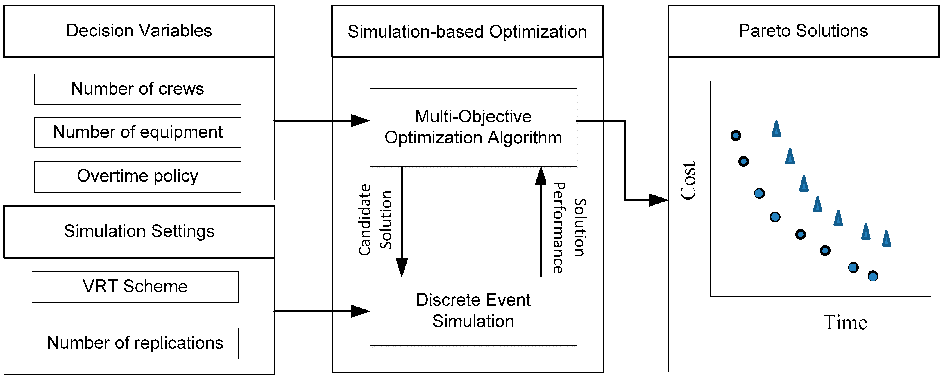
The current study builds on the simulation optimization framework developed in our previous work [41,43]. Figure 1 illustrates the proposed DES optimization framework, which is intended to support decision-makers in enhancing current practices in the construction industry. The primary objective of the framework is to minimize the project duration and cost by identifying a set of near-optimal decision variables. The framework consists of three main phases: input, analysis, and output. In the input phase, the decision variables of the optimization problem and the settings of the simulation are identified. The decision variables are variables that have an impact on the project duration and cost, such as the number of crews and overtime policies. Each decision variable has a defined range and incremental value from which the optimization algorithm will generate candidate solutions. On the other hand, the simulation settings require the decision maker to identify the VRT scheme (CRN, AV, CAV) to be used and the number of simulation replications for evaluating the candidate solutions. The second phase is the simulation-based optimization. In this phase, there are two distinctive, interconnected, and iterative processes. The first process is the optimization algorithm. In this study, the fast messy Genetic Algorithm (fmGA) [44] is employed as the metaheuristic optimization algorithm to find the optimal solutions for the project. The fmGA searches the decision-variable space and produces candidate solutions through genetic operators. The algorithm then passes these candidate solutions to the DES engine, which is the second process. Stochastic DES estimates the duration and cost of each candidate solution, considering the combination of decision variables, the VRT scheme, and the number of simulation replications. The performance (duration and cost) of each solution is returned to the optimization algorithm. This phase keeps iterating between these two processes till the termination criteria are met. The final phase of this framework is the output phase. In this phase, the framework generates a Pareto front comprising non-dominated optimal solutions. These Pareto solutions (PSs) illustrate the trade-offs between project duration and cost. Each PS corresponds to a specific resource allocation strategy required to achieve a particular combination of project duration and total cost.

The main expected advantages of this framework are as follows: (1) to evaluate candidate solutions using a lower number of simulation replications, thereby reducing the overall computational burden associated with solving the DES-based optimization problem; and (2) to enhance the quality and optimality of the generated Pareto solutions. This section consists of three subsections: random number management, DES optimization integration, and performance metrics.

3.1. Random Number Management

The implementation of VRTs require careful management of the random numbers used when evaluating candidate solutions. This is achieved by synchronizing the random-number streams across different uncertain events (i.e., stochastic tasks) in a simulation model. A random number stream is a continuous sequence of random numbers generated from a specific starting point called a seed number. In each replication, random numbers for each stochastic task are obtained either from a dedicated random number stream (same-stream method) or by assigning a new random number stream (new-stream method). To distinguish between these two methods, the former is identified by appending the subscript “ss” to the abbreviated name (i.e., CRN_ss, AV_ss, and CAV_ss), whereas the latter is identified by appending the subscript “ns” to the abbreviated name (i.e., CRN_ns, AV_ns, and CAV_ns). Irrespective of the adopted method, identifying the required number of random numbers (RRNs) for each stochastic task is critical for determining the minimum stream length. The length must be sufficient to generate the RRN while avoiding overlapping with other streams. Once a random number is consumed by a task, it is not reused during the simulation of a candidate solution, thereby ensuring independence and preventing unintended correlation across stochastic tasks. The stochastic task with the largest RRN determines the overall stream length. Equation (1) is used to compute the maximum RRN required for each VRT.

$$\mathit{arg} {max}_i {RRN}_i={Inst}_i\times {RNU}_i\times N \forall i=\mathrm{1,2},\dots ,I$$

(1)

where RRN_i denotes the required number of random numbers for stochastic task i; Inst_i represents the total number of instances of task i generated within a single replication; RNU_i is the number of random numbers used to generate a single random variate for task i; and N is the total number of replications performed. Under the new-streams method, N is set to 1. The value of RNU varies from one probability distribution to another [45].

As mentioned previously, the synchronization of the random number streams is crucial for ensuring both statistical independence and controlled correlation. The level of synchronization depends on the selected technique. For example, CRN requires synchronization across stochastic tasks, simulation replications, and candidate solutions. On the other hand, AV uses paired replications with complementary random numbers to reduce variability within each solution. When these two techniques are combined, a higher level of coordination is required to maintain both effects simultaneously.

Table 1. Synchronization requirements for each adopted VRT.

Synchronization Between	VRT			Purpose
	CRN	AV	CAV
Tasks	x	x	x	Statistical Independence
Replications or pairs	x	x	x	Statistical Independence
Replications within pairs	N/A	x	x	Negative Correlation
Candidate solutions	x	N/A	x	Positive Correlation

summarizes the synchronization requirements for each technique.

Regardless of the implemented technique, independent random-number streams are assigned to each stochastic task to avoid unintended dependencies within the simulation model. That is, no two stochastic tasks will share the random numbers during the simulation. In the same-streams method, each stochastic task continues from the last random numbers used in the previous replication, ensuring consistency across replications. In contrast, the new-streams method assigns a new, unused random-number stream to each stochastic task, maintaining independence between replications while avoiding any overlap in random numbers between tasks. To ensure that no two replications reuse the same random numbers under the new-streams method, the starting point of each replication is determined based on unused portions of the random-number streams. This guarantees statistical independence where required.

When AV or CAV are used, simulations are executed in pairs. Within each pair, the second replication is generated using complementary random numbers relative to the first. This induces a negative correlation between the two replications, which reduces variability in the estimated performance of each solution. Finally, when CRN or CAV are applied, the same initial seed number is used when evaluating different candidate solutions. This introduces a positive correlation between solutions, which reduces the variance in the estimated objective functions between the solutions. These synchronization strategies are necessary to control the structure of randomness in the simulation, enabling the intended variance reduction effects.

3.2. DES Optimization Algorithms

As previously discussed, fmGA is the adopted optimization algorithm, while DES is used to estimate the duration and cost associated with each candidate solution. Algorithm 1 presents a summary of the algorithm used to incorporate CRN into the DES optimization framework. First, the algorithm generates and stores a random seed number. Then, the optimization algorithm generates the initial population. Each solution in this population is subsequently evaluated through DES. Within the DES model, the stored seed number is applied consistently across all solutions to generate the random-number streams used by the stochastic tasks during the first simulation replication (j), as shown in line 7 of Algorithm 1. As mentioned in Section 2.1, if the same-streams method is used, then subsequent replications resume from the last random numbers used in the preceding replication, see line 8 of Algorithm 1. If the new-streams method is used, streams will be generated using the first random number from an unused stream, as shown in line 12 of Algorithm 1. Once the number of replications is reached, the simulation engine will calculate the average duration and cost of each solution. After evaluating all the solutions within a population, the fmGA will sort the solutions based on their fitness and apply genetic operators to generate a new population. Each generation follows the same sequence of steps: evaluating solutions using DES, sorting the population based on performance, and applying genetic operators to produce a new population. This procedure is repeated iteratively until the predefined termination condition is met. Once the termination condition is satisfied, the framework outputs a set of PS.

Algorithm 1. DES optimization algorithm under CRN
1	Generate and save seed number
2	Initialize population
3	FOREACH population until termination DO
4	FOREACH solution in a population
5	Run simulation
6	IF same stream is used THEN
7	IF j = 1 Then generate streams using seed number
8	ELSE continue from last random number
9	END IF
10	ELSE
11	IF j = 1 THEN generate streams using seed number
12	ELSE generate streams using unused random number
13	END IF
14	END IF
15	Calculate duration and cost
16	Sort population and apply genetic operators
17	RETURN Pareto solutions

Algorithm 2 shows the summary of the algorithm for incorporating AV and CAV into DES optimization. The algorithm is similar to the one used for CRN. The main difference is that replications are run in pairs (p) with complementary random numbers. When AV is used, the algorithm will generate a random seed number for each solution. This number is used as the basis for generating the random number streams. On the other hand, all candidate solutions evaluated using CAV will use the same random seed number to generate the streams, as shown in line 1 of Algorithm 2. If the new-streams method is used, streams will be generated using the first random number from an unused stream in the standard replication, as shown in line 16 of Algorithm 2.

Due to the implementation of VRT in estimating the project duration and cost, additional simulation replications are required to obtain statistically sound estimates for the PS. Accordingly, each Pareto solution is re-evaluated using a large number of independent replications (e.g., 1000 replications). Finally, non-dominated sorting is applied to these re-evaluated solutions, and the resulting set constitutes the final Pareto front.

Algorithm 2. DES optimization algorithm under AV and CAV
1	Generate seed number. Save it if CAV is used
2	Initialize population
3	FOREACH population until termination DO
4	FOREACH solution in a population
5	Run simulation
6	IF same stream is used THEN
7	FOREACH standard replication
8	IF p = 1 Then generate streams using seed number
9	ELSE continue from last random number
10	END IF
11	FOREACH antithetic replication
12	Use complimentary random numbers
13	ELSE
14	FOREACH standard replication
15	IF p = 1 Then generate streams using seed number
16	ELSE generate streams using unused random number
17	END IF
18	FOREACH antithetic replication
19	Use complimentary random numbers
20	Calculate duration and cost
21	Sort population and apply genetic operators
22	RETURN Pareto solutions

3.3. Performance Metrics

In this study, three performance metrics are used to evaluate the effectiveness of incorporating VRTs into DES optimization. The first metric, shown in Equation (2), quantifies the time savings achieved through the use of VRTs, reflecting the reduction in overall computational time required to complete the optimization process [41,42].

$$T_s={\displaystyle \frac{T_{IR}-T_{VRT}}{T_{IR}}}\times 100$$

(2)

$T_s$ is the achieved time savings; $T_{IR}$ and $T_{VRT}$ are the times required to solve the optimization problem using independent replications (IRs) and VRT, respectively.

The second performance metric is the hypervolume indicator. This metric, originally proposed by Zitzler [46], is widely utilized to examine the performance of multiobjective evolutionary algorithms. This indicator calculates the volume of the space that a Pareto front dominates [47]. When evaluating several Pareto fronts, a larger hypervolume indicator is considered superior, as it reflects both higher solution optimality and greater diversity [48]. Once the indicator is estimated for each scheme, Equation (3) is used to quantify the relative improvement achieved through the use of VRTs.

$$∆HV={\displaystyle \frac{{HV}_{IR}-{HV}_{VRT}}{{HV}_{IR}}}\times 100$$

(3)

where $∆HV$ denotes the percentage difference in the hypervolume indicator, ${HV}_{IR}$ and ${HV}_{VRT}$ represents the hypervolume indicator obtained using IR and VRT, respectively.

The third performance metric, presented in Equation (4), is the percentage of inferior solutions (ISs) obtained by each scheme [41]. To identify inferior solutions, the set of PSs generated under each scheme is re-evaluated through many independent replications (i.e., 1000 replications). The superior solutions for each scheme are then identified through non-dominated sorting. A lower percentage of inferior solutions indicates a higher overall quality of the corresponding optimization scheme.

$$IS={\displaystyle \frac{{IS}_{scheme}}{{PS}_{scheme}}}\times 100$$

(4)

3.4. Framework Implementation

STROBOSCOPE release 4.2.0.0, a simulation platform specifically developed for modeling construction operations, was used to develop the discrete event simulation model [45]. The optimization problem was solved using the Darwin optimization framework version 0.91 [49] that employs the fmGA. The genetic algorithm is responsible for generating candidate solutions while STROBSOCOPE calculates the project duration and cost. STROBOSCOPE has embedded functions and tools that facilitate the implementation of the selected VRT. For example, the modeler can assign a specific random-number stream to any task or function in the model. In this study, all stochastic tasks are assigned independent streams to ensure controlled and consistent random sampling. More details about the implementation can be found in [41,42,43].

4. Case Study

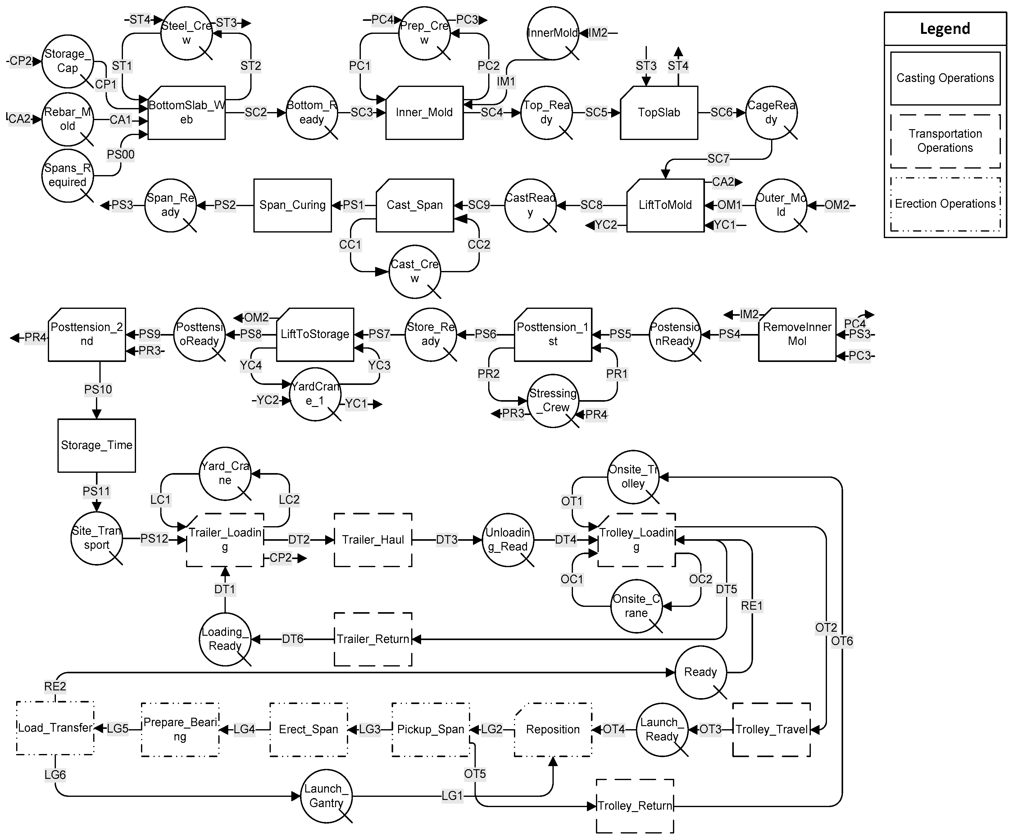
The case study involves the construction of a precast box-girder bridge using the full-span launching gantry method. The superstructure consists of 35 identical spans, each with a length of 25 m. Figure 2 illustrates the developed simulation model. The construction process consists of three main operations: (1) casting operations, where each span is constructed off-site, (2) transportation operations, which reflect moving the completed spans to the construction site, and (3) erection operations, where transported spans are placed in their final location using a launching gantry. The simulation begins by setting up the queues that store the resources required for construction activities. Using a rebar mold and a steel crew, the reinforcing steel and tendon ducts of the bottom section of the slab are installed. Once this is complete, a preparation crew will insert an inner mold on top of the already completed bottom section. A steel crew then proceeds to place the reinforcement for the top section of the slab, after which the completed rebar cage is lifted into an outer mold using a yard crane. At this point, the span is ready for casting. Next, a casting crew pours concrete to form the span, which is then allowed to cure. After curing, the inner mold is removed, and a stressing crew carries out the first stage of post-tensioning. The span is subsequently transferred to a storage area using a yard crane, where the second stage of post-tensioning is completed. The span is then stored on site until it is transported to the construction site. This step concludes the casting operations. Once the set storage time has elapsed, a trailer is then loaded with the precast concrete box girder span and transported to the bridge construction site. Once the launching gantry is ready, an on-site crane unloads the span from the trailer and places it onto a trolley. The trailer then returns to the precast yard for reloading. Meanwhile, the trolley moves the span to the designated launching location. Upon arrival, the erection operations start with the launching gantry adjusting its position and lifting the span from the trolley. The trolley then returns for the next load, which represents the last step of the transportation operations. At the same time, the gantry installs the span in its final position. Finally, the permanent bearings are grouted, and the load of the span is transferred from the temporary supports to the permanent bearings.

Table 2 presents the durations of tasks adopted in the model. The project cost is computed as a function of the overall project duration and the number of resources assigned to each solution. The simulation model was verified and validated by tracking the flow of entities and examining the random number streams generated under each technique, thereby ensuring correct model logic and proper synchronization of random numbers [50].

The case study considers 13 decision variables that influence both project duration and cost [41]. These variables are (1) number of delivery trucks, (2) distance between the casting yard and the construction site access point, (3) number of rebar cage molds, (4) number of inner molds, (5) number of outer molds, (6) number of preparation crews, (7) number of stressing crews, (8) number of steel crews, (9) number of casting crews, (10) curing method, (11) overtime policy, (12) storage capacity of the casting yard, and (13) storage time of each span in the casting yard. Table 3 presents the value ranges and increments for 11 of these decision variables. Two curing methods, regular curing and accelerated curing, are considered, each affecting the project duration and cost. Additionally, 15 overtime policies were adopted from RS Means [51].

Table 2. Duration of the tasks used in the simulation model.

Task	Duration (Minutes)	Task	Duration (Minutes)
BottomSlab_Web	Triangular [640, 961, 1280] *	Trailer_Haul	F (Distance, Speed)
Inner_Mold	Triangular [120, 300, 480] *	Trolley_Loading	Triangular [30, 60, 90] **
TopSlab	Triangular [660, 984, 1300] *	Trailer_Return	F (Distance, Speed)
LiftToMold	Triangular [23, 45, 68]	Trolley_Travel	F (Distance, Speed)
Cast_Span	Triangular [520, 771, 1020] *	Reposition	Triangular [120, 240, 360] **
Span_Curing	(600 or 1200) *	Pickup_Span	Triangular [30, 60, 90]**
RemoveInnerMol	Triangular [90, 255, 420] *	Trolley_Return	F (Distance, Speed)
Posttension_1st	Triangular [120, 300, 480] *	Erect_Span	Triangular [120, 240, 360] **
LiftToStorage	Triangular [30, 60, 90] **	Trolley_Return	F (Distance, Speed)
Posttension_2nd	Triangular [120, 300, 480] *	Prepare_Bearing	Triangular [120, 240, 360] **
Trailer_Loading	Triangular [30, 60, 90] **	Load_Transfer	Triangular [30, 60, 90] **

* Adapted from [52]; ** adapted from [53].

Table 2. Duration of the tasks used in the simulation model.

Task	Duration (Minutes)	Task	Duration (Minutes)
BottomSlab_Web	Triangular [640, 961, 1280] *	Trailer_Haul	F (Distance, Speed)
Inner_Mold	Triangular [120, 300, 480] *	Trolley_Loading	Triangular [30, 60, 90] **
TopSlab	Triangular [660, 984, 1300] *	Trailer_Return	F (Distance, Speed)
LiftToMold	Triangular [23, 45, 68]	Trolley_Travel	F (Distance, Speed)
Cast_Span	Triangular [520, 771, 1020] *	Reposition	Triangular [120, 240, 360] **
Span_Curing	(600 or 1200) *	Pickup_Span	Triangular [30, 60, 90]**
RemoveInnerMol	Triangular [90, 255, 420] *	Trolley_Return	F (Distance, Speed)
Posttension_1st	Triangular [120, 300, 480] *	Erect_Span	Triangular [120, 240, 360] **
LiftToStorage	Triangular [30, 60, 90] **	Trolley_Return	F (Distance, Speed)
Posttension_2nd	Triangular [120, 300, 480] *	Prepare_Bearing	Triangular [120, 240, 360] **
Trailer_Loading	Triangular [30, 60, 90] **	Load_Transfer	Triangular [30, 60, 90] **

* Adapted from [52]; ** adapted from [53].

The case study is divided into two subsequent parts. The first focuses on the pilot study and the associated sensitivity analysis, whereas the second provides a comparative assessment of the various optimization schemes.

Table 3. Ranges of decision variables.

Decision Variable	Min	Max	Increment
Number of delivery trucks (NDTs)	1	20	1
Precast yard distance (km) (PYD)	10	100	10
Number of rebar cage molds (NRCs)	1	20	1
Number of inner molds (NIMs)	1	20	1
Number of outer molds (NOMs)	1	20	1
Number of preparation crews (NPCs)	1	20	1
Number of stressing crews (NSCs1)	1	20	1
Number of steel crews (NSCs2)	1	20	1
Number of casting crews (NCCs)	1	20	1
Precast yard storage capacity (PYS)	1	50	5
Storage time (h) (ST)	1	84	1

Table 3. Ranges of decision variables.

Decision Variable	Min	Max	Increment
Number of delivery trucks (NDTs)	1	20	1
Precast yard distance (km) (PYD)	10	100	10
Number of rebar cage molds (NRCs)	1	20	1
Number of inner molds (NIMs)	1	20	1
Number of outer molds (NOMs)	1	20	1
Number of preparation crews (NPCs)	1	20	1
Number of stressing crews (NSCs1)	1	20	1
Number of steel crews (NSCs2)	1	20	1
Number of casting crews (NCCs)	1	20	1
Precast yard storage capacity (PYS)	1	50	5
Storage time (h) (ST)	1	84	1

4.1. Pilot Study and Sensitivity Analysis

A pilot study using three random solutions, listed in Appendix A, was conducted to evaluate the success of implementing the selected VRT. The success is measured by variance reduction and induced correlation. These solutions were evaluated using the three VRTs: CRN, AV, and CAV. Each VRT was tested under the two random-number stream assignment methods and then compared with IR. The purpose of the comparison is to calculate the reduced variance resulting from implementing VRTs. To ensure proper calculation, two IR scenarios were implemented: one using single replications and another using pairs of replications, which mimic the structure used in AV. When IR simulations are conducted in pairs, each pair consists of two replications with independent random numbers. A sensitivity analysis was then performed to determine the appropriate number of simulation replications or pairs required for evaluating candidate solutions during the DES optimization process. For CRN, 10, 15, 20, 30, 40, and 50 replications were tested. For AV and CAV, the number of pairs tested was set to half the number of corresponding replications (i.e., 5, 7, 10, 15, 20, and 25). In total, 36 different configurations were analyzed in this study.

Four performance metrics are used to assess the improvements achieved by the implemented schemes [41]. The first metric is the average reduction in variance ($\overline{∆S^2}$) among the three solutions, when a VRT is applied in place of IR. The second metric is the average induced correlation ($\overline{\rho }$), which evaluates the effectiveness of each VRT in introducing the desired correlation between paired simulations. The third metric quantifies the average reduction in the margin of error $(\overline{∆E(\propto )})$, commonly known as the half-width of the confidence interval, among the three solutions. The fourth metric estimates the average number of replications $(\overline{J_E})$ that would be required under IR to attain the same margin of error achieved through the application of the VRT schemes. These equations are well-established in the simulation literature and can be found in many standard references on variance reduction and simulation output analysis, such as [2].

Table 4. Results summary of pilot study and sensitivity analysis.

		CRNss		CRNns		AVss		AVns		CAVss		CAVns
J (p)	Metric	D	C	D	C	D	C	D	C	D	C	D	C
10 (5)	$\overline{∆S^2}(\%)$	90	78	83	57	78	84	57	82	87	94	81	90
	$\overline{∆E}(\%)$	68	54	60	38	54	61	42	60	63	75	57	70
	$\overline{\rho }$	0.92	0.84	0.88	0.57	−0.23	0.43	−0.01	0.29	−0.13	0.71	0.21	0.52
	$\overline{J_E}$	102	56	198	17	23	40	36	47	38	84	27	70
15 (7)	$\overline{∆S^2}(\%)$	88	69	84	64	76	71	72	70	81	83	84	88
	$\overline{∆E}(\%)$	73	57	70	55	52	48	49	49	57	60	61	67
	$\overline{\rho }$	0.91	0.72	0.84	0.70	−0.20	0.22	0.30	0.50	0.30	0.44	0.22	0.43
	$\overline{J_E}$	135	55	228	27	31	31	39	42	49	55	57	74
20 (10)	$\overline{∆S^2}(\%)$	89	74	85	72	70	78	69	82	72	88	81	83
	$\overline{∆E}(\mathrm{\%})$	78	66	75	65	46	53	46	59	50	66	58	60
	$\overline{\rho }$	0.90	0.73	0.83	0.73	0.04	−0.02	0.16	0.40	0.12	0.44	0.41	0.16
	$\overline{J_E}$	189	81	269	31	35	47	41	70	61	93	82	76
30 (15)	$\overline{∆S^2}(\%)$	88	75	87	73	79	79	85	84	85	86	88	87
	$\overline{∆E}(\mathrm{\%})$	81	73	81	72	54	54	61	61	63	64	67	65
	$\overline{\rho }$	0.87	0.74	0.82	0.78	−0.06	0.03	0.16	0.25	0.11	0.22	0.26	0.36
	$\overline{J_E}$	276	122	513	50	72	75	108	120	160	140	212	140
40 (20)	$\overline{∆S^2}(\%)$	81	74	84	71	75	80	85	80	86	82	88	86
	$\overline{∆E}(\mathrm{\%})$	81	77	82	75	50	55	61	56	63	57	67	64
	$\overline{\rho }$	0.82	0.73	0.82	0.74	−0.04	0.06	0.07	0.14	0.10	0.10	0.27	0.33
	$\overline{J_E}$	324	159	554	57	80	104	135	111	214	110	261	161
50 (25)	$\overline{∆S^2}(\%)$	75	72	85	72	79	80	84	81	85	80	86	86
	$\overline{∆E}(\mathrm{\%})$	80	79	85	78	54	55	60	57	61	56	65	64
	$\overline{\rho }$	0.79	0.73	0.80	0.71	−0.05	0.09	0.18	0.08	0.00	0.09	0.14	0.35
	$\overline{J_E}$	308	185	672	66	122	128	163	148	195	127	352	201

Note: D = project duration; C = project cost.

exhibits the mean values of the three-performance metrics computed across the three pilot-study candidates. In each comparison, the VRT configurations and the corresponding IR scenarios used the same number of replications (or pairs). For instance, when all three solutions were run using CRN and IR for 15 replications, the average variance of the duration-mean differences was reduced by 88%. Likewise, the average half-width of the 90% confidence interval for the was reduced by 73%. The average induced correlation between replications when estimating project duration was 0.91. Additionally, achieving an equivalent level of variance reduction under IR would require approximately 135 replications. Similarly, one can interpret the remaining results in Table 4. Based on the results of the pilot study, all three VRTs reduced the variance and the margin of error across the different numbers of replications (pairs). Although AV and AV_ns were successful in reducing the variance, they did not always induce a negative correlation among the tested solutions. Thus, the pilot study demonstrates that both CRN and CAV can effectively replace IR for the purposes of this paper. Nevertheless, all three VRTs are incorporated into the full optimization experiments to comprehensively evaluate their influence on the efficiency and performance of the simulation-optimization model.

4.2. Comparison of the Different Schemes

Table 5. fmGA parameters used in the case study.

Parameter	Value
Cut rate	0.017
Splice rate	0.6
Mutation rate	0.015
Random seed	0.5
Population size	100
Generations per era	500
Number of eras	2
Maximum trials	100,000
Size of search space	6.4512 × 1015

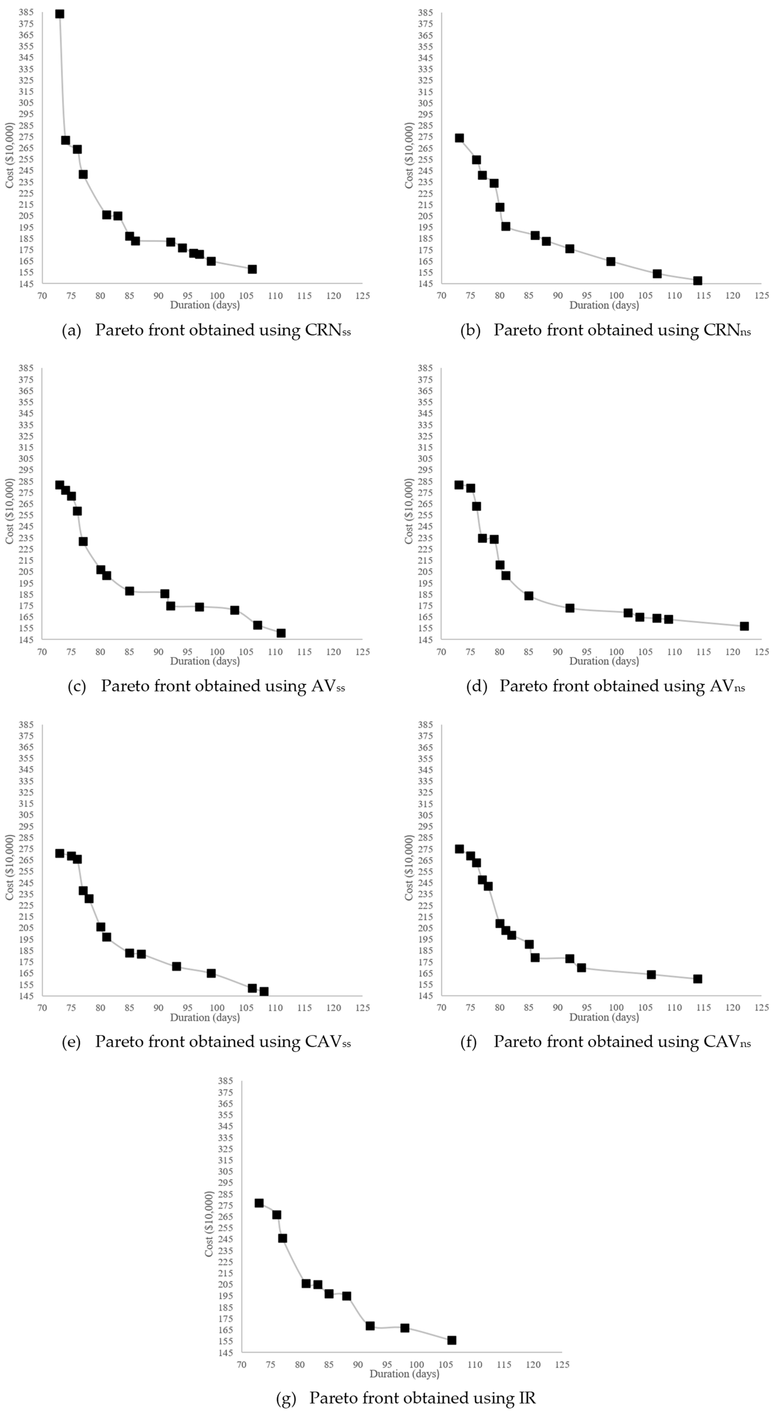
summarizes the fmGA parameters adopted in this study. For each VRT, a total of 100,000 candidate solutions were evaluated. All experiments were conducted using a workstation with an Intel Core i7 quad-core processor running at 3.4 GHz and 16 GB of RAM. The framework successfully generated a set of PS from each scheme. The PS were, then, re-evaluated using 1000 simulation replications. Figure 3 presents the final Pareto fronts generated using CRN, AV, CAV, and the IR baseline. These fronts illustrate the non-dominated trade-offs between minimizing project duration and cost. All four techniques produced Pareto fronts that are closely aligned, indicating consistent convergence performance across the methods. The corresponding decision variable values and objective function results for each technique are provided in Appendix A.

Table 6. Summary of the performance metrics results.

Technique	N	P	T (Hours)	Ts (%)	HV	ΔHV (%)	IS (%)
IR	100	---	7.20	---	7004	---	38
CRNss	10	---	1.37	80.97	7036	0.47	26
AVss	---	5	1.33	81.53	7160	2.24	13
CAVss	---	5	1.33	81.53	7368	5.21	7
CRNns	10	---	1.27	82.36	7265	3.74	20
AVns	---	5	1.28	82.22	7038	0.50	18
CAVns	---	5	1.28	82.22	7162	2.27	0

N = number of replications; P = number of pair runs.

summarizes the performance metric results obtained in this study. The simulation setup employed ten replications for CRN, five paired replications for AV and CAV, and 100 replications for IR. The application of VRTs enabled evaluating the solutions using fewer simulation replications while still obtaining a reliable estimate of their objective functions, thereby decreasing overall computational time. Specifically, the IR-based optimization required 7.20 h to complete, whereas the VRT-based approaches required approximately 1.31 h, corresponding to an average time savings of 81.81% relative to IR. The VRT schemes also produced higher-quality optimal solutions than IR, as reflected in improvements in the hypervolume indicator. On average, the VRT schemes achieved a 2.4% increase in hypervolume relative to IR. Furthermore, the VRT schemes yielded a lower proportion of inferior solutions within the Pareto front. When VRTs were used, an average of 14% of the Pareto solutions were classified as inferior, compared with 38% under IR. Thus, the use of VRTs improved solution optimality by reducing the proportion of inferior solutions in the Pareto fronts by an average of 63.15%. To this end, using any of the VRT schemes would result in better computational performance and higher quality solutions. However, it is also important to consider how the VRT schemes fared against each other. The same-streams method required a slightly longer time to complete compared to the new-streams method. CRN_ns performed better than CRN_ss on the hypervolume indicator and rate of inferior solutions. On the other hand, AV_ss outperformed AV_ns on these two metrics. However, the random-number stream method had a noticeable, yet inconsistent, impact when CAV is used. For example, CAV_ss have a much higher hypervolume indicator when compared to CAV_ns. On the other hand, CAV_ns had fewer inferior solutions presented compared to CAV_ss. Out of three VRT methods, CAV outperformed CRN and AV regardless of which stream method is implemented.

5. Discussions

The main objective of this study was to evaluate the improvements achievable by implementing CRN, AV, and CAV within a construction simulation optimization framework. Previous work has established that using CRN in simulation optimization can reduce the computational time of the optimization process. This study extends prior work by demonstrating that AV and CAV not only improve computational efficiency but also enhance optimization outcomes in complex construction planning problems. This represents an important distinction from prior work, where VRTs have primarily been viewed as tools for improving estimation accuracy rather than as mechanisms that directly affect optimization performance. These improvements were measured relative to the baseline case where IR is used. Using IR as a baseline is the de facto standard against which the effectiveness of VRTs in reducing the variance is measured [9]. In this sense, IR represents a valid baseline, making it appropriate for assessing the improvements introduced by the implemented VRT.

The results provide additional insight into the performance of the three techniques relative to one another. While all used VRTs have an almost equal computing efficiency, their performance on the other two metrics varied across the random-number stream management methods. The same-streams method took slightly longer to complete than the new-streams method. CRN performed better under the new-stream method, whereas AV performed better using the same-stream method. However, the random-number stream method had a noticeable, yet inconsistent, impact when CAV is used. For example, CAV_ss have a much higher hypervolume indicator than CAV_ns. On the other hand, CAV_ns presented fewer inferior solutions than CAV_ss. The use of CAV yielded the fewest inferior solutions among the three techniques, regardless of the stream management method, suggesting greater robustness in the presence of noisy objective functions.

The results highlight two key aspects of performance improvement. First, implementing VRTs led to an 81.81% reduction in computational time. While this timesaving may appear modest in isolation, it adds significant value within the broader context of the field of construction simulation optimization. The time saved can be used to evaluate more solutions, thereby increasing confidence in the optimization outcomes. Moreover, the planning of such complex projects can occur multiple times during their lifecycle; as such, a shorter evaluation time supports faster turnaround for time-sensitive decisions. In this sense, the primary benefit of VRTs lies in enabling the solution of larger, more complex construction optimization problems that would otherwise be computationally prohibitive within practical limits.

Second, the improvement in solution quality and optimality has direct practical relevance. These improvements are measured using two metrics: the Hypervolume indicator and percentage of inferior solutions. The observed increase in the hypervolume indicator shows that the implemented techniques covered a larger region of the objectives’ space and provided more diversity. For example, the IR approach yielded 10 optimal solutions, whereas the applied techniques yielded 12–14 optimal solutions. The lowest-cost solution from CRN and CAV was approximately 4.5% cheaper than the lowest-cost solution from IR. This cost saving can help increase the appeal of simulation optimization as a planning tool for the construction industry. On the other hand, the optimization algorithm generated fewer inferior solutions when VRTs were implemented. This reduction suggests that VRTs can enhance the robustness of the optimization process by mitigating the noise in stochastic simulation outputs, thereby enabling more informed decision-making in practice.

Although the results suggest that the implementation of VRTs can improve the quality of optimal solutions, it is important to consider the limitations of the underlying simulation model. The objective functions used in this study are stochastic estimates based on assumed input distributions, cost functions, and modeling assumptions. The extent to which these improvements translate into practice depends on the accuracy of the model, the quality of input data, and the representation of real-world uncertainty. Nonetheless, using the same optimization algorithm and problem settings, the improvements achieved remain valuable.

Despite these promising results, several limitations should be acknowledged. The findings are based on the presented case study, and their generalizability to other types of construction problems warrants further investigation. The application of the VRTs requires performing a pilot study to ensure its success in reducing the variance. The sensitivity analysis and calculation of reduced variance and induced correlation reported in the pilot study were conducted manually. In addition, implementing VRTs requires careful handling of random-number streams, which may increase modeling complexity.

6. Conclusions

This study investigated the implementation of three VRTs, which are CRN, AV, and CAV, within a stochastic DES optimization framework for construction operations. Each VRT was evaluated under the same-streams and new-streams methods, and their effectiveness was assessed through a case study. The primary limitation of existing stochastic DES optimization frameworks in construction is their computational time, coupled with their susceptibility to generating inferior solutions due to noise introduced during the evaluation of candidate solutions. In contrast to previous studies where VRTs were used to improve simulation accuracy, this study provides valuable insights into the role of VRT in improving the performance of optimization algorithms when coupled with stochastic simulation.

The results demonstrated three important conclusions: (1) VRTs enhanced the quality of optimal solutions by dominating a larger area of the objectives’ space and providing a more diverse solutions as measured by the Hypervolume indicator; (2) VRTs significantly reduced the number of inferior solutions presented in the final Pareto front as measured by the percentage of inferior solutions; and (3) VRTs permitted using fewer simulation replications to estimate the objective functions which in turn led to huge reduction in computational time. By increasing both efficiency and reliability, VRTs facilitate the evaluation of more alternatives and support more informed decision-making in complex and uncertain project environments. These outcomes have the potential to broaden the application of simulation optimization in planning construction projects.

Future work should focus on testing the proposed approach on a wider range of construction problems to generalize its benefits. Additionally, automating the generation of the pilot study using STROBOSCOPE can also encourage the implementation of VRTs. This work could contribute to better adoption of simulation-optimization in the industry and enable informed decision-making.