Modeling and Analysis of Key Structural Parameters of Infrared Line Drawing Device for Oil and Gas Pipeline Cutting Operations

Abstract

To address the issues associated with traditional multi-point surveying processes in the dead-end cutting for oil and gas pipelines—such as cumbersome procedures, high error rates, lengthy emergency repair cycles, and difficulties in ensuring welding precision—an infrared line drawing device has been developed that enables rapid positioning, long-distance high-precision alignment, and accurate marking of cutting locations. This paper establishes mathematical models for the centering deflection mechanism and the marking mechanism, and derives theoretical solutions for key structural parameters. Thirteen finite element models were constructed using Abaqus to simulate operating conditions involving different pipe diameters and link lengths. A variance-based uniformity metric was employed to quantify structural stress stability, and optimal parameters were determined based on the principle that smaller variance indicates more uniform stress distribution and closer to ideal component service life. The results indicate that the optimal length of the three mounting bolts is 85 mm, with a maximum deflection angle of 9.25°, which meets the requirements. A spring extension of 5 mm for the marking pen can accommodate the compensation needs for marking on DN300 to DN500 pipes. An optimal set of connecting rod parameters across pipe diameters has been determined, with a 240 mm connecting rod capable of covering more than 75% of operating conditions. This device and its parameters are expected to contribute to first-pass compliance and reduce downtime, providing efficient and precise technical support for the maintenance and emergency repair of oil and gas pipelines.

1. Introduction

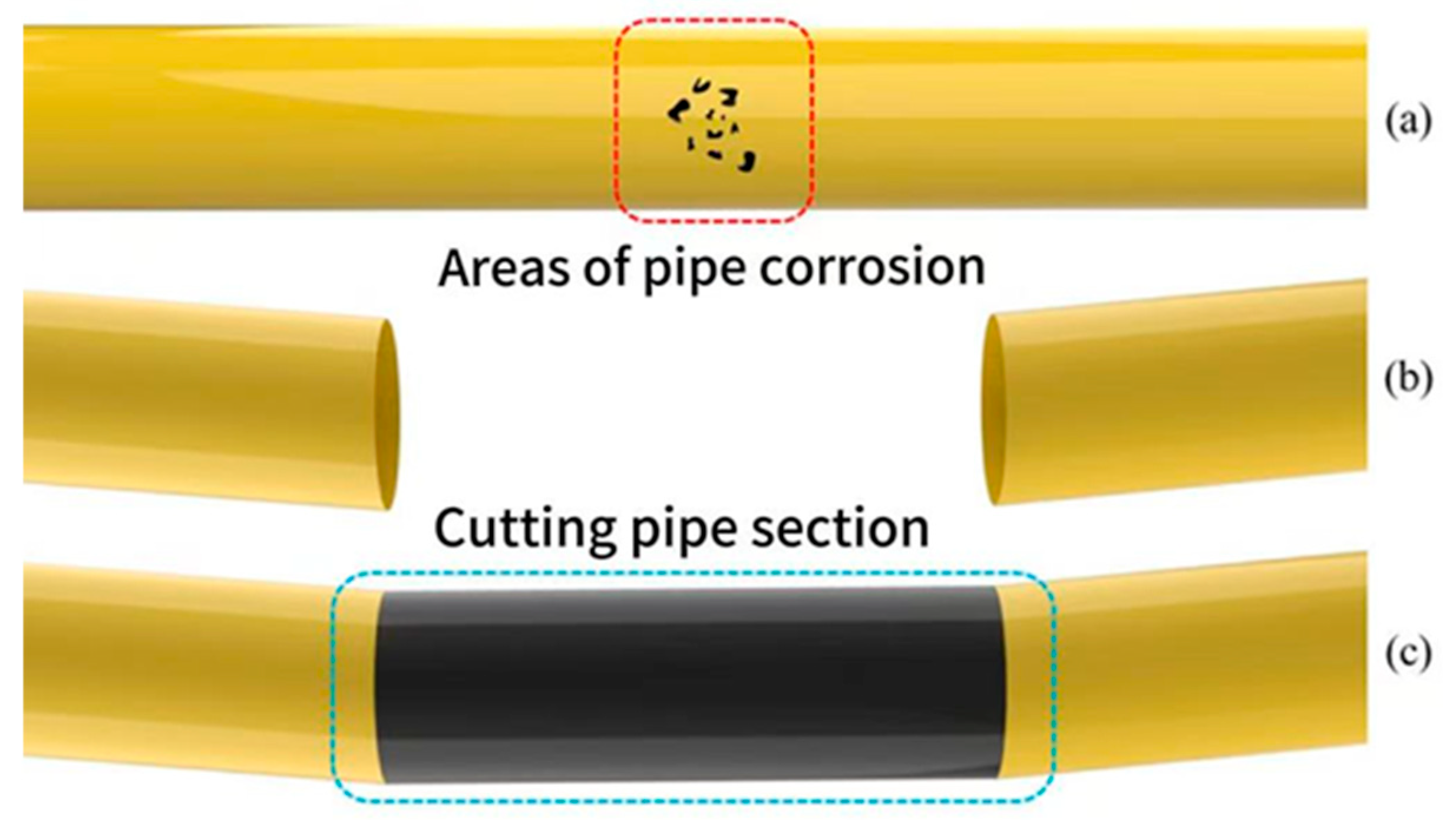
During the service life of oil and gas pipelines, defective sections caused by corrosion [1,2,3], cracks [4,5,6], or mechanical damage [7] frequently require removal and replacement to ensure structural integrity and operational safety. Pipeline corrosion, as illustrated in Figure 1a, is one of the most common defects leading to section replacement [8,9,10,11]. After cutting out the damaged segment, residual stresses in the pipe wall often cause lateral or angular misalignment between the two free pipe ends [12,13,14,15]. To address this issue, dead-end cutting technology is widely applied to determine accurate cutting positions [16], as shown in Figure 1b. Following precise cutting, a new straight pipe spool is inserted and welded between the two ends, with the final repaired configuration presented in Figure 1c.

Dead-end cutting technology demands a high degree of precision, traditional methods often require extensive calculations, which in turn rely on large amounts of data obtained through manual measurements. These cumbersome procedures not only prolong emergency repairs but also compromise accuracy [17]. During emergency repairs on gas pipelines, it is essential to minimize gas service interruptions as much as possible and to complete the cutting and pipe replacement operations at the dead-end section quickly and accurately in order to minimize losses [18,19,20,21]. Conventional multi-point surveying methods require cutting both pipe ends into straight, square-ended sections. However, due to variations in the skill levels of the operators, errors in multi-point measurements were significant, resulting in notable discrepancies between the cross-sections at both ends [22]. In particular, when there is a significant difference in elevation along the pipeline centerline, the multi-point surveying process becomes more cumbersome and time-consuming [23]. Surveying errors can directly affect the quality of the welding process, potentially leading to various welding defects and delaying the start of production [24,25,26]. To overcome the limitations of manual multipoint surveying, a variety of alternative technologies have been explored in recent years. Motta et al. [27] developed a laser-based pipe end measurement system that automatically inspects the outer diameter, inner diameter, and wall thickness of pipes. This system enables more efficient pipe alignment before welding and effectively reduces Hi-Lo mismatch. Bao Xiaohua et al. [28] presented a non-contact laser measuring approach for underground pipeline diameter detection, which achieves high-precision pipeline dimension acquisition with a simplified device layout and low site dependency. Shammazov et al. [16] proposed a laser scanning method to accurately assess pipeline position within a repair trench. From the generated point cloud data, a polynomial describing the bending of the pipeline’s central axis can be derived, allowing precise determination of the cutting position prior to installation of a new spool. Despite these advances, such techniques often require bulky equipment or extensive on-site preparation, limiting their practicality for rapid emergency repairs in field conditions. Consequently, finding ways to expedite the cutting and alignment process, minimize cumulative errors, and achieve first-pass compliance—thereby reducing gas shutdown time and resuming production as quickly as possible—has become a long-standing goal in the oil and gas pipeline construction industry [29,30].

This paper systematically calculates and analyzes the key structural parameters of an infrared line drawing device. Based on mathematical models of the centering deflection mechanism and the marking mechanism, theoretical solutions for the key structural parameters were derived. By simulating 13 sets of finite element models under different operating conditions and using a variance-based uniformity metric to quantify parameter stability in multi-pipe configurations, the optimal link parameters for each pipe diameter were ultimately determined.

2. Calculation of Key Structural Parameters for Infrared Line Drawing Device

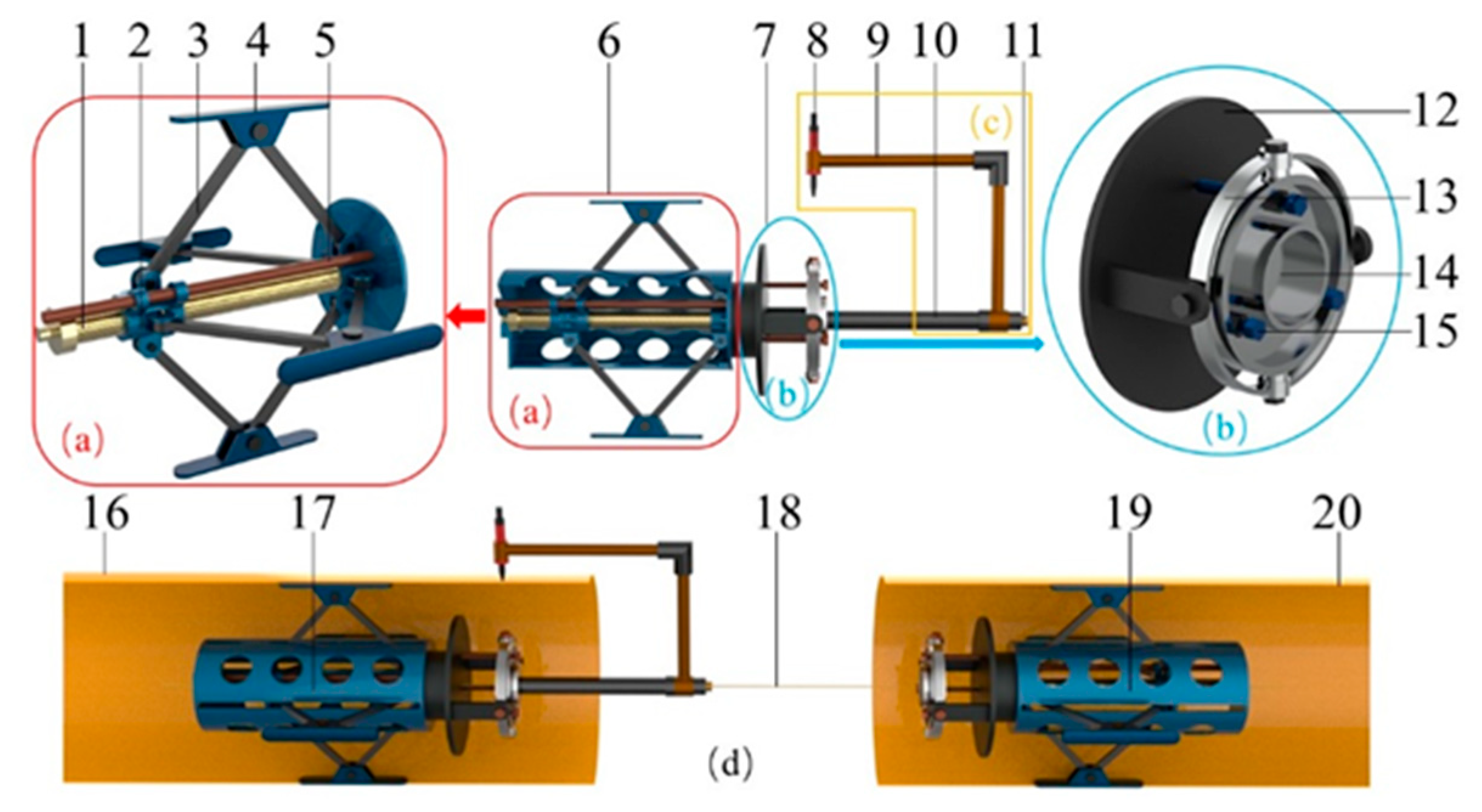
The overall structure of the infrared line drawing device is shown in Figure 2, where (a) represents the support mechanism, (b) represents the centering deflection mechanism, and (c) represents the marking mechanism. The structural dimensions of the device are shown in

Table 1. Table of structural dimensions.

Name	Dimensions/mm
Total length of the device	799
Total height of the device	452
Cylinder length	356
Cylinder diameter	159
Length of the laser emitter	300
Mounting plate diameter	186
Rotating plate diameter	150

.

The overall structure and operating principle of the infrared line drawing device are as follows. At the location of a dead-end break in the pipeline, the support mechanism at the emitter end of the marking device is inserted into the interior of the pipeline. Turning the hexagonal coupling drives the trapezoidal threaded rod to rotate; the threaded rod is fitted with a threaded sleeve that mates with its trapezoidal threads. A guide rod is mounted on the threaded sleeve to provide guidance, enabling the axial displacement of the threaded sleeve along the trapezoidal threaded rod. Both the threaded sleeve and the mounting plate are equipped with connecting rod structures, allowing the connecting rods to engage with them and achieve relative rotation. The axial displacement of the threaded sleeve is transmitted through the connecting rods to four support plates, driving the support plates to press against the inner wall of the pipeline, thereby completing the support and fixation of the launch-end support mechanism. Once secured, remove the centering deflection mechanism from the transmitter end of the marking device. Using the threaded connection between the mounting plate and the rotating base, install the centering deflection mechanism onto the transmitter-end support mechanism. The core component of this mechanism is a rotating disc, whose center is connected to an annular groove; the centerline of the annular groove passes through the center of the rotating disc and is perpendicular to the end face of the rotating disc. Install the laser emitter into the annular groove; at this point, all preliminary preparations for the emitter end are complete. The preliminary preparation process for the receiver end of the marking device is identical to that of the emitter end. First, insert the receiver-end support mechanism into the interior of the receiver-end pipe, and rotate the hexagonal joint to securely fix the connecting rod and support plate against the inner wall of the pipe. Subsequently, install the receiver-end centering deflection mechanism onto the receiver-end support mechanism to complete the preliminary preparations for the receiver end. Mount the laser pointer onto the laser emitter at the transmitter end and adjust the emitter’s angle based on the emitted laser beam. Since the laser emitter is installed in the annular groove of the rotating disk, and leveraging the structural characteristics of the rotating disk and rotating ring, the emitter can rotate freely within a 360-degree range while the center position of the rotating disk remains constant throughout the rotation. Align the laser with the center of the rotating disk at the receiver end to complete the long-distance laser alignment of the marking device. After completing the long-distance laser alignment, tighten the three mounting bolts on the centering deflection mechanism at the transmitter end to fully secure the mounting plate. Then, install the marking mechanism onto the laser emitter at the transmitter end. As the marking mechanism rotates once around the laser emitter, the marking pen traces a smooth, continuous elliptical curve on the outer wall of the transmitter-end pipe, thereby determining the cutting position for the fixed pipe at the transmitter end. Remove the marking mechanism and laser emitter from the emitter end, install the laser emitter onto the receiver end turntable, and then mount the marking mechanism onto the receiver end laser emitter. Rotate the marking mechanism once around the laser emitter; the marking pen will trace a smooth, continuous elliptical curve on the outer wall of the receiver end pipe, thereby determining the cutting position for the fixed pipe at the receiver end. After determining the butt-cut positions for both ends of the pipe, remove the marking device to prevent damage to the equipment during the cutting process. Install the cutting machine to cut the pipe, and select a cylindrical pipe segment with a diameter matching the shortest straight-line distance between the cut ends for cutting. Weld the cylindrical pipe segment to the cut pipe to complete the butt-cut assembly and welding operation.

2.1. Derivation of Structural Parameters for the Centering Deflection Mechanism

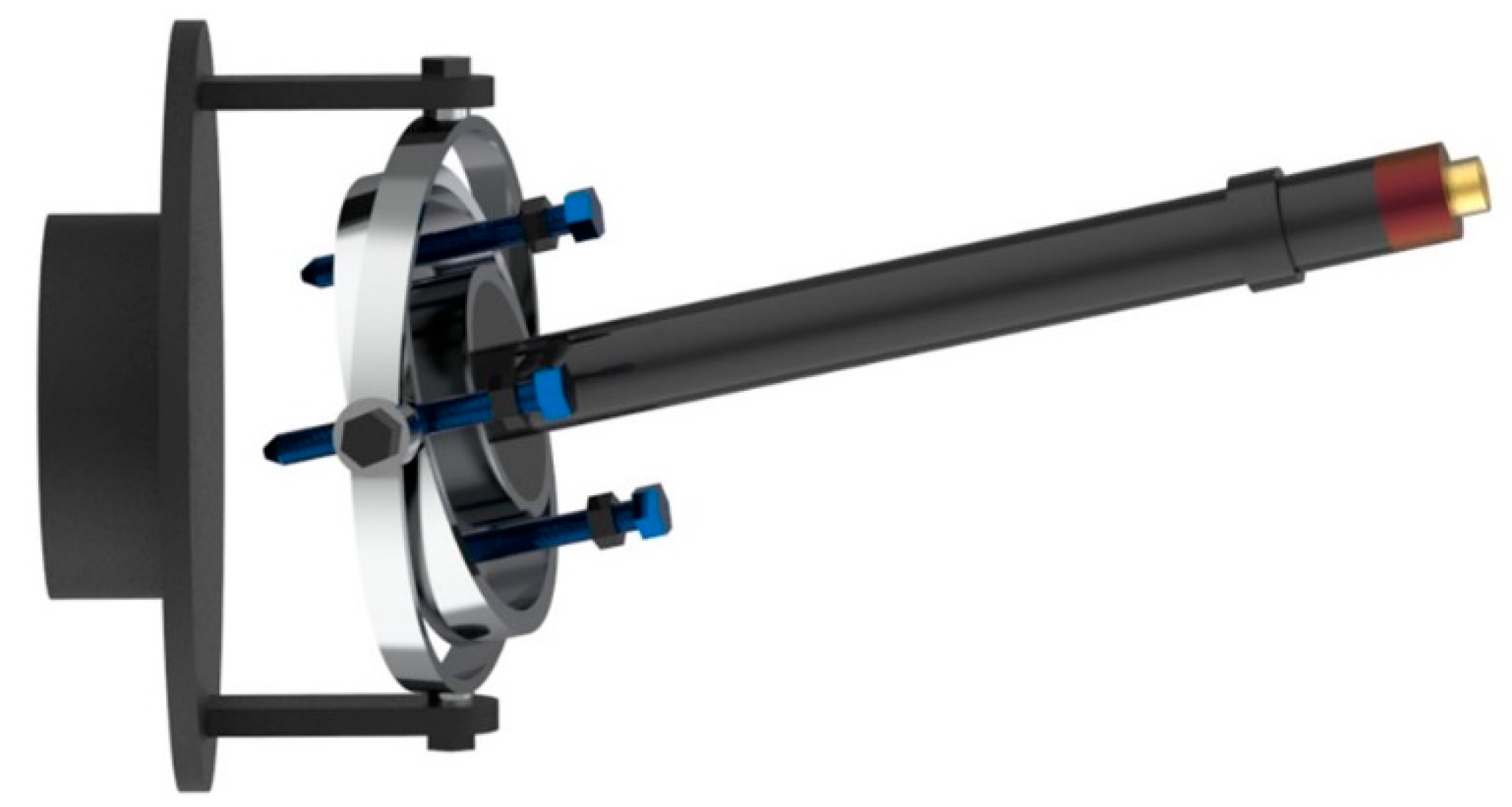
The core function of the centering deflection mechanism in an infrared line drawing device is to achieve high-precision, long-distance alignment between fixed points on the central axes of the pipes at both ends. Its structural parameters must be designed based on the pipe offset. Figure 3 shows the centering deflection mechanism in its fixed position inside the pipe.

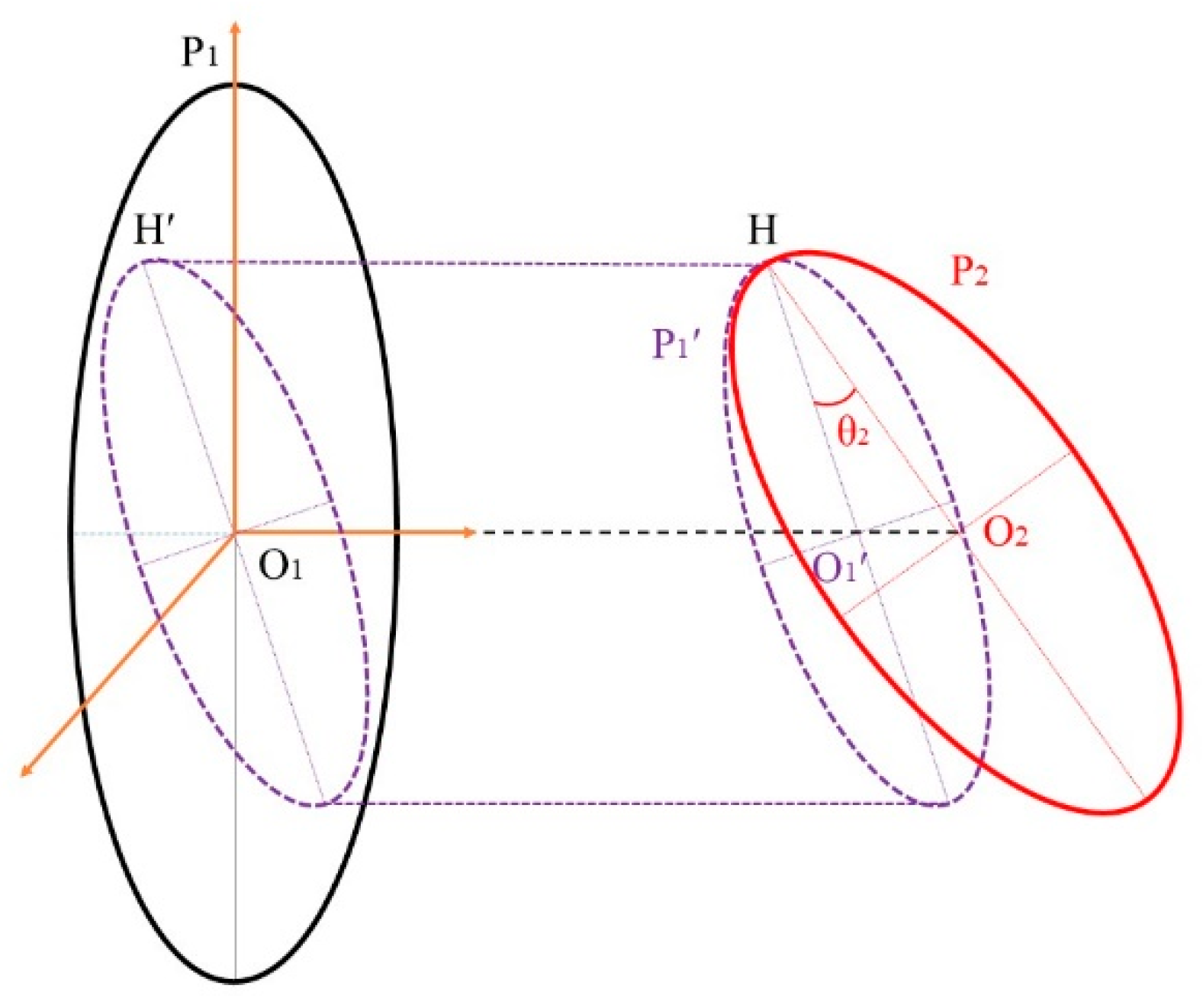
The following geometric assumptions are clearly defined: (1) Planes P₁ and P₂ are regarded as circular disks; (2) The projection is an orthogonal projection.

Based on the operating principle of the centering deflection mechanism, it is evident that this mechanism enables the laser emitter to be deflected in any direction in space while maintaining proper alignment. The laser emitter is mounted vertically at the center of the rotating disk. After long-distance alignment is completed, the rotating disk is secured using three mounting bolts. Therefore, studying the deflection angle of the laser emitted by the laser emitter is equivalent to studying the spatial relationship between the plane containing the rotating plate (plane P₂) and the plane containing the mounting plate (plane P₁). A simplified model of this is shown in Figure 4.

The center of plane P₁ is point O₁, and the center of plane P₂ is point O₂. The line segment O₁O₂, connecting the centers of the two planes, is perpendicular to plane P₁ and has a length of 75 mm. Let H be the point on plane P₂ closest to plane P₁. Draw a plane P₁′ parallel to plane P₁ through point H, with its center O₁′ lying on line segment O₁O₂. The angle between planes P₁ and P₂ in space is then equal to the angle θ₂ between planes P₁′ and P₂.

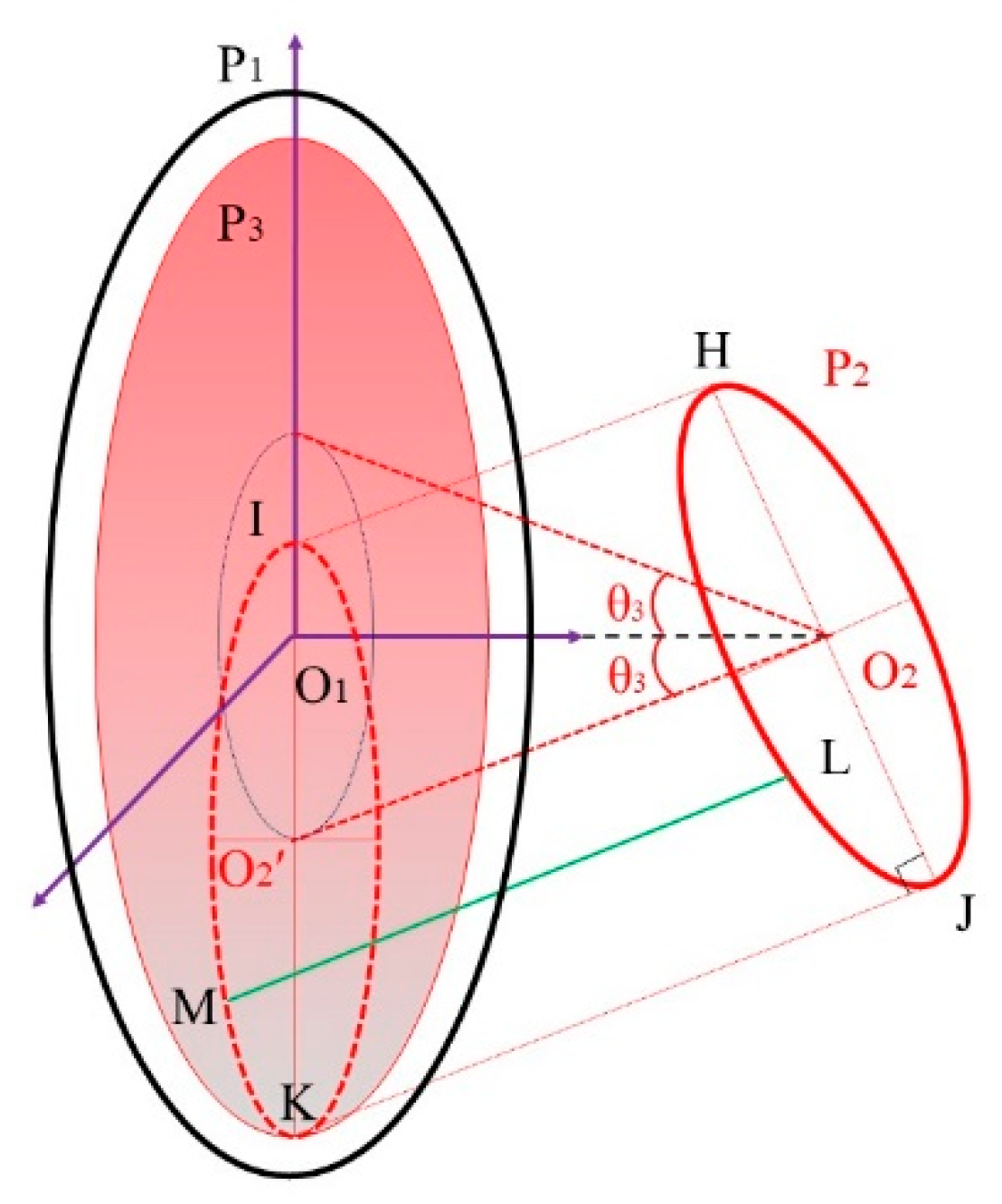
For ease of analysis, a coordinate system is established using the major axis and minor axis of surface P₁, as well as the line containing O₁O₂. In the centering deflection mechanism of the drawing device, the turntable is secured by three mounting bolts perpendicular to the plane of the turntable. The support condition of the three fixing bolts can be represented as the set of points on the edge of surface P₂, with radius HO₂, that lie on the shortest distance from surface P₂ to surface P_1, as shown in Figure 5.

The plane P₂ on which the rotating disk lies has its center at O₂. The projection of plane P₂ onto plane P₁ is an elliptical surface with center O₂′; the line segment O₂O₂′ is perpendicular to plane P₂. Point L is an arbitrary point on the boundary of plane P₂, and point M is the corresponding point on the boundary of the projection plane, such that the line segment LM is perpendicular to plane P₂. As point L moves along the edge of surface P₂, the length of segment LM changes. When point L moves to point H, the length of segment LM equals HI, at which point LM takes its minimum value. When point L moves to point J, the length of segment LM equals JK, at which point LM takes its maximum value. The center point O₂′ of the projected surface rotates with point O₁ as the center and segment O₁O₂′ as the radius, forming a circular path. As O₂′ moves along this trajectory, the entire area covered by the projection plane is the circular surface P₃ with point O₁ as its center and segment O₁K as its radius.

The three fixing bolts are evenly distributed on the rotating disk and are fixed in position. According to the principle that three points determine a plane [31], although the positions of the bolts are fixed, their lengths can be adjusted via threaded connections, thereby allowing plane P₂ to rotate freely within a certain angle. Therefore, the length of the bolts directly determines the maximum allowable rotation angle of the rotating disk. Let segment LM represent the length of one of the bolts. As shown in Figure 5, within the half-plane containing O₂J, the farther point L is from point J, the longer segment JK becomes, and the larger the angle between planes P₁ and P₂. Since the bolt length LM is fixed, to ensure that plane P₂ achieves maximum deflection capability in any direction, point L must be placed at the position of point J. At this point, the shortest distance from every point on surface P₂ to the projection plane along a direction perpendicular to P₂ is less than JK; the corresponding deflection angle is the maximum deflection angle θ_3max that surface P₂ can achieve in any direction. The relationship between bolt length LM and the maximum deflection angle θ_3max is:

$${\mathrm{L}\mathrm{M}}_{\mathrm{m}\mathrm{a}\mathrm{x}}=\mathrm{J}\mathrm{K}$$

(1)

$${\mathrm{O}}_1{\mathrm{O}}_2+\mathrm{H}{\mathrm{O}}_2{\sin \mathsf{\theta }}_{3\mathrm{m}\mathrm{a}\mathrm{x}}=\mathrm{J}\mathrm{K}{\cos \mathsf{\theta }}_{3\mathrm{m}\mathrm{a}\mathrm{x}}$$

(2)

The maximum deflection angle θ_3max can be calculated using Equation (2). The relationship between the maximum value of the radius KO₁ of the circular maximum projection area P₃ and the distance O₁O₂ from the center of the mounting plate to the center of the rotating plate, as well as the distance HO₂ from the three mounting bolts to the center of the rotating plate, is as follows:

$${\mathrm{H}\mathrm{O}}_2={\mathrm{J}\mathrm{O}}_2$$

(3)

$${\mathrm{K}\mathrm{O}}_1={\mathrm{O}}_1{\mathrm{O}}_2^{\mathrm{’}}+{\mathrm{K}\mathrm{O}}_2^{\mathrm{’}}$$

(4)

$${{\mathrm{K}\mathrm{O}}_1}_{\mathrm{m}\mathrm{a}\mathrm{x}}={\mathrm{O}}_1{\mathrm{O}}_2\tan {\mathsf{\theta }}_{3\mathrm{m}\mathrm{a}\mathrm{x}}+{\displaystyle \frac{{\mathrm{J}\mathrm{O}}_2}{{\cos \mathsf{\theta }}_{3\mathrm{m}\mathrm{a}\mathrm{x}}}}$$

(5)

$${{\mathrm{K}\mathrm{O}}_1}_{\mathrm{m}\mathrm{a}\mathrm{x}}={\mathrm{O}}_1{\mathrm{O}}_2\tan {\mathsf{\theta }}_{3\mathrm{m}\mathrm{a}\mathrm{x}}+{\displaystyle \frac{{\mathrm{H}\mathrm{O}}_2}{{\cos \mathsf{\theta }}_{3\mathrm{m}\mathrm{a}\mathrm{x}}}}$$

(6)

2.2. Calculation of Structural Parameters for the Centering Deflection Mechanism

As can be seen from the derived parameters, the length of the three mounting bolts is a key factor affecting the deflection angle of the laser emitter. Since the distance from the three mounting bolts to the center of the rotating disk and the dimensions of the mounting plate are fixed, this paper focuses primarily on determining the optimal length of the three mounting bolts. In the designed centering deflection mechanism, the mounting plate has a radius of 93 mm, the distance between O₁ and O₂ is 75 mm, and the distance from the axis of the three mounting bolts to the center of the rotating disk is 55 mm.

To investigate the relationship between the length of the three fixing bolts and the maximum deflection angle, the bolt length was set within a range of 75 mm to 85 mm, with increments of 1 mm. The deflection angles and maximum fixing radii for different bolt lengths were calculated, and the results are shown in

Table 2. Summary of centering deflection structural parameters.

LM/[mm]	θ3/[°]	O1K/[mm]
75	0.00	55.00
76	0.97	56.28
77	2.05	57.72
78	3.00	59.01
79	3.93	60.28
80	4.93	61.68
81	5.84	62.96
82	6.70	64.19
83	7.60	65.49
84	8.44	66.74
85	9.25	67.95

.

According to the calculation data in Table 1, when the length of the three mounting bolts exceeds 75 mm, the centering deflection mechanism can be securely fixed. As the bolt length increases, both the maximum swivel angle and the fixing radius gradually increase. Since the mounting plate has a radius of 93 mm, if the maximum radius of the fixed position on the mounting plate exceeds 93 mm, the fixed position of the three mounting bolts will extend beyond the maximum area of the mounting plate, making it impossible to achieve the deflection fixation of the centering deflection mechanism. Therefore, the optimal length of the three fixing bolts is 85 mm, corresponding to a maximum deflection angle of 9.25°. At this point, the fixing radius of 67.95 mm is less than the mounting plate radius, allowing the mechanism to be securely fixed in the deflected position.

2.3. Derivation of Structural Parameters for the Marking Mechanism

The core function of the marking mechanism in an infrared line drawing device is to determine the cutting path where a plane passing through the two fixed points and perpendicular to the line connecting them intersects with the pipe, after achieving long-distance alignment of the fixed points on the centerlines of the two pipe ends. Its structural parameters must be designed based on the pipe’s nominal diameter and offset. 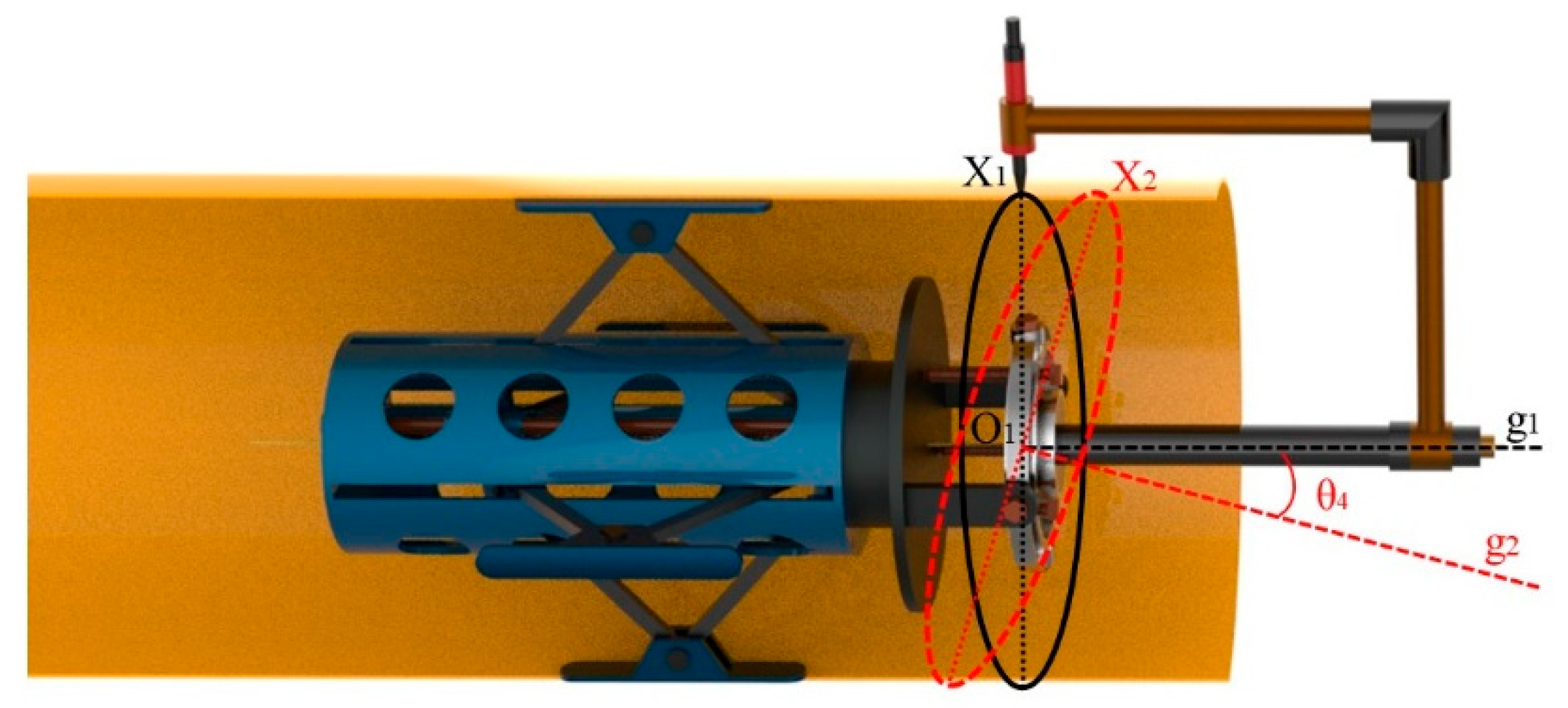Figure 6 illustrates the operating state of the marking mechanism on the outer surface of the pipe.

Once the marking device has completed the long-distance alignment of the support, mounting, and centering mechanisms, the marking mechanism can be installed and used to mark the outer surface of the pipe. The straight line O₁g₁ represents the central axis of the laser emitter, and point O₁ is the center of the mounting plate. The marking trajectory formed by the marking mechanism on the outer surface of the pipe is X₁, with point O₁ as its center; the central axis O₁g₁ is perpendicular to the plane containing the trajectory X₁. When the laser emitter is deflected by an angle θ₄, its central axis becomes the line O₁g₂. At this point, the marking trajectory X₂ formed by the marking mechanism on the outer wall of the pipe is an elliptical path, with point O₁ remaining as its center and the central axis O₁g₂ perpendicular to the plane containing the trajectory X₂. Since the central axis O₁g₁ coincides with the pipe’s own central axis, the trajectory X₁ drawn on the outer wall of the pipe at this time is a perfect circle; let the radius of this circle be R₁. When the laser emitter is deflected, the plane containing the marking pen rotates accordingly, so the trajectory drawn on the outer wall of the pipe becomes an ellipse X₂. The length of the minor axis of this ellipse remains equal to R₁; let the length of its major axis be R₂. The radius R₁ of trajectory X₁ and the length R₂ of the major axis of trajectory X₂ satisfy:

$${\mathrm{R}}_2={\displaystyle \frac{{\mathrm{R}}_1}{\cos {\mathsf{\theta }}_4}}$$

(7)

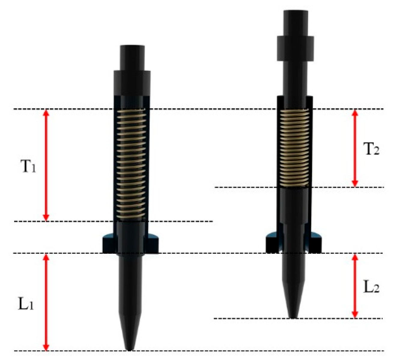
When the marking mechanism traces an elliptical path on the outer surface of a pipe, if the major axis of the ellipse exceeds the diameter of the pipe’s outer surface, the marking pen must be equipped with a telescoping function to compensate for the difference between the major axis of the ellipse and the diameter of the pipe’s outer surface. The internal structural parameters of the marking pen are shown in Figure 7. Let the initial length of the internal spring be T₁, and the initial length of the pen tip be L₁. During the process of drawing the elliptical trajectory, the pen tip is compressed, causing the spring to compress, at this point, the length of the pen tip becomes L₂, and the length of the spring becomes T₂. The maximum compression achievable by the marking pen is equal to the difference between the major and minor axes of the elliptical trajectory, denoted as R_C.

2.4. Calculation of Structural Parameters for the Marking Mechanism

Based on parametric derivations, marking accuracy is influenced by the nominal diameter of the pipeline and the compression of the marking pen. This paper investigates the extension range of the marking pen for pipelines of different nominal diameters. Pipelines with nominal diameters of DN300, DN350, DN400, DN450, and DN500 were selected, and a deflection angle of θ = 10° was set to calculate the spring extension range. The results are shown in

Table 3. Spring travel range data table.

DN/[mm]	R1/[mm]	θ/[°]	R2/[mm]	RC/[mm]
300	162.5	10	165	2.5
350	188.5	10	191.4	2.9
400	213	10	216.3	3.3
450	240	10	243.7	3.7
500	265	10	269.1	4.1

.

Analysis of the data in the table shows that when θ = 10°, the spring compression (R_C) increases with the nominal diameter, with the DN500 pipe corresponding to a maximum compression of 4.1 mm. This requires that the extension range of the spring in the marking mechanism of the infrared line drawing device must be greater than 4.1 mm, and the length of the marking pen tip must be greater than 4.1 mm. Taking into account factors such as dirt on the pipe’s outer wall, the marking pen tip is designed to be 5 mm long, with a spring travel distance of 5 mm, which can meet the marking requirements for DN300 to DN500 pipes.

3. Multi-Pipe Adaptive Parameter Analysis

In actual pipeline emergency repair operations, due to limitations in manpower and transportation, it is difficult to accurately equip damaged pipelines with nominal diameters ranging from DN300 to DN500 with infrared line drawing device featuring the optimal connecting rod parameters. Although the connecting rods of existing infrared line drawing devices can be disassembled and reassembled to switch between different length parameters, frequent on-site replacement of connecting rods prolongs the repair cycle and reduces operational efficiency. To address this engineering challenge, this paper conducts a cross-diameter adaptability study for five nominal pipe diameters—DN300, DN350, DN400, DN450, and DN500—and their corresponding optimal link parameters of 140 mm, 170 mm, 190 mm, 240 mm, and 270 mm. By substituting various connecting rod parameters into finite element models of the five nominal diameter pipes, this study systematically investigates the applicability of different connecting rod lengths under multi-diameter combination conditions, thereby determining the optimal structural parameters for connecting rods across the range of pipe diameter combinations.

Define connecting rod lengths of 140 mm, 170 mm, 190 mm, 240 mm, and 270 mm, and pipe nominal diameters of DN300, DN350, DN400, DN450, and DN500. The following data was used for analysis to calculate the connecting rod angle, axial thrust, input torque, and individual bolt preload corresponding to different length parameters, as shown in

Table 4. Summary of adaptive structural parameters for multi-pipe.

Nominal Diameter	Connecting rod Length/[mm]	Vertical Angle α/[°]	Horizontal Angle β/[°]	Axial Thrust Q/[N]	Input Torque M/[N·mm]	Bolt Tensile Force FL/[N]	End Distance n/[mm]
DN300	140	48.92	41.08	1549.688	9653.006	387.422	273.946
DN300	170	57.24	32.76	1686.758	10,506.813	421.689	199.091
DN300	190	61.04	28.96	1811.851	11,286.018	452.963	152.518
DN300	240	67.46	22.54	2168.080	13,504.973	542.020	41.667
DN300	270	70.08	19.92	2396.161	14,925.688	599.040	−22.685
DN350	140	33.31	56.69	1672.555	10,418.344	418.139	331.234
DN350	170	46.51	43.49	1537.353	9576.175	384.338	238.334
DN350	190	51.99	38.01	1582.091	9854.842	395.523	185.594
DN350	240	60.82	29.18	1803.394	11,233.340	450.848	65.901
DN350	270	64.32	25.68	1965.536	12,243.326	491.384	−1.666
DN400	140	—	—	—	—	—	—
DN400	170	33.35	56.65	1671.452	10,411.472	417.863	298.067
DN400	190	41.64	48.36	1545.859	9629.154	386.465	232.524
DN400	240	53.72	36.28	1609.274	10,024.169	402.319	98.032
DN400	270	58.27	31.73	1716.035	10,689.184	429.009	25.714
DN450	140	—	—	—	—	—	—
DN450	170	10.78	79.22	4177.788	26,023.443	1044.447	421.408
DN450	190	28.48	61.52	1831.190	11,406.480	457.797	303.771
DN450	240	45.91	44.09	1535.989	9567.673	383.997	140.262
DN450	270	51.79	38.21	1579.401	9838.088	394.850	60.684
DN500	140	—	—	—	—	—	—
DN500	170	—	—	—	—	—	—
DN500	190	—	—	—	—	—	—
DN500	240	36.87	53.13	1599.188	9961.339	399.797	197.000
DN500	270	44.67	45.33	1535.319	9563.502	383.830	105.337

In the table, “—” indicates that the length of the connecting rod does not meet the minimum requirement for the pipe support mechanism corresponding to the nominal diameter, making it impossible to secure the pipe with internal supports. Rows highlighted in red represent parameter sets where the vertical angle of the connecting rod is less than the minimum required value (34.85°), leading to mechanical interference between the rods. Rows highlighted in purple represent parameter sets where the distance from the center of the threaded sleeve to the end of the guide rod is less than the minimum required value (30 mm), leading to interference between the threaded sleeve and the outer casing.

.

Since none of the above three scenarios can achieve the required support and fixation of the support mechanism, they must be discarded, and finite element calculations and analysis must be performed on the remaining 13 data sets.

3.1. Establishment of Finite Element Model

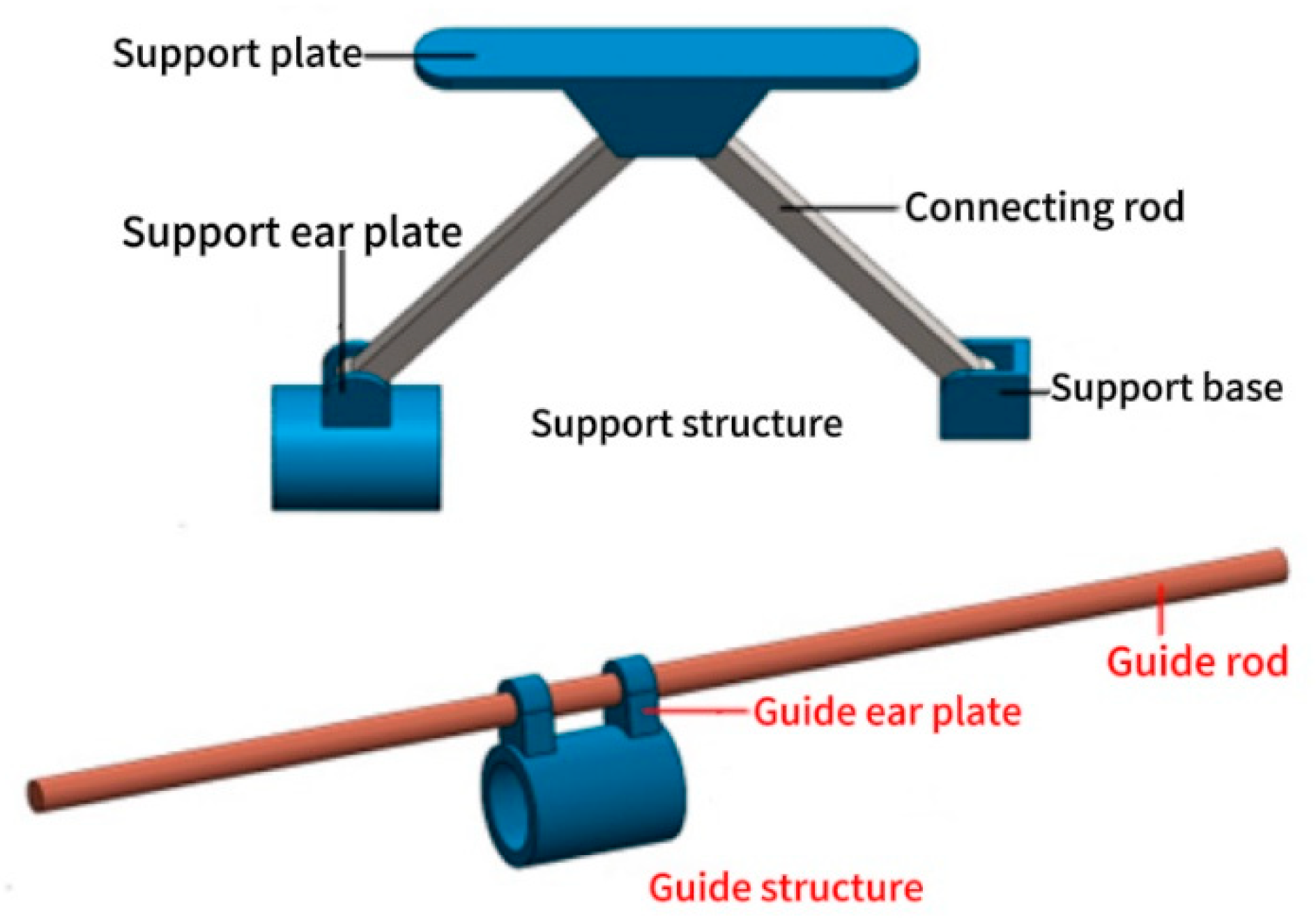
The support mechanism of the infrared line drawing device is divided into two parts: the support structure and the guide structure. The support structure consists of a support plate, a connecting rod, a support ear plate, and a support base, while the guide structure consists of a guide rod and a guide ear plate, as shown in Figure 8. The connecting rod, support plate, support ear plate, support base, guide rod, and guide ear plate are all made of Q245 steel, with a density of 7800 kg/m³, a Poisson’s ratio of 0.3, and a Young’s modulus of 210 GPa. The material parameters are shown in

Table 5. Material parameters for key components.

Name	Material	Density/[kg/m3]	Young’s Modulus/[MPa]	Poisson’s Ratio
connecting rod	Q245	7800	210,000	0.3
support plate	Q245	7800	210,000	0.3
support base	Q245	7800	210,000	0.3
support ear plate	Q245	7800	210,000	0.3
guide rod	Q245	7800	210,000	0.3
guide ear plate	Q245	7800	210,000	0.3

. Under operating conditions, the stress level remains below the yield strength, indicating that the material is in the linear elastic stage. Therefore, a linear elastic constitutive model was employed in the finite element analysis.

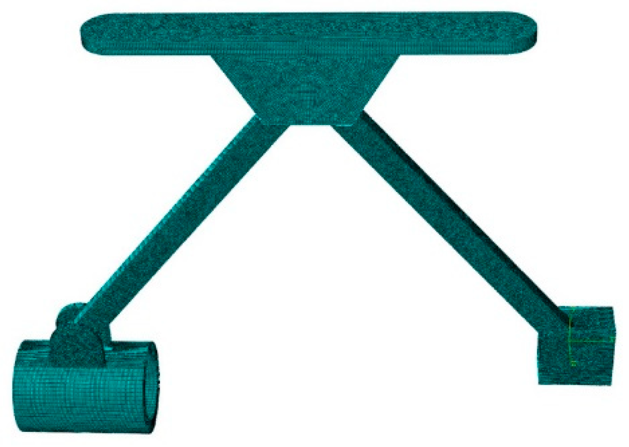
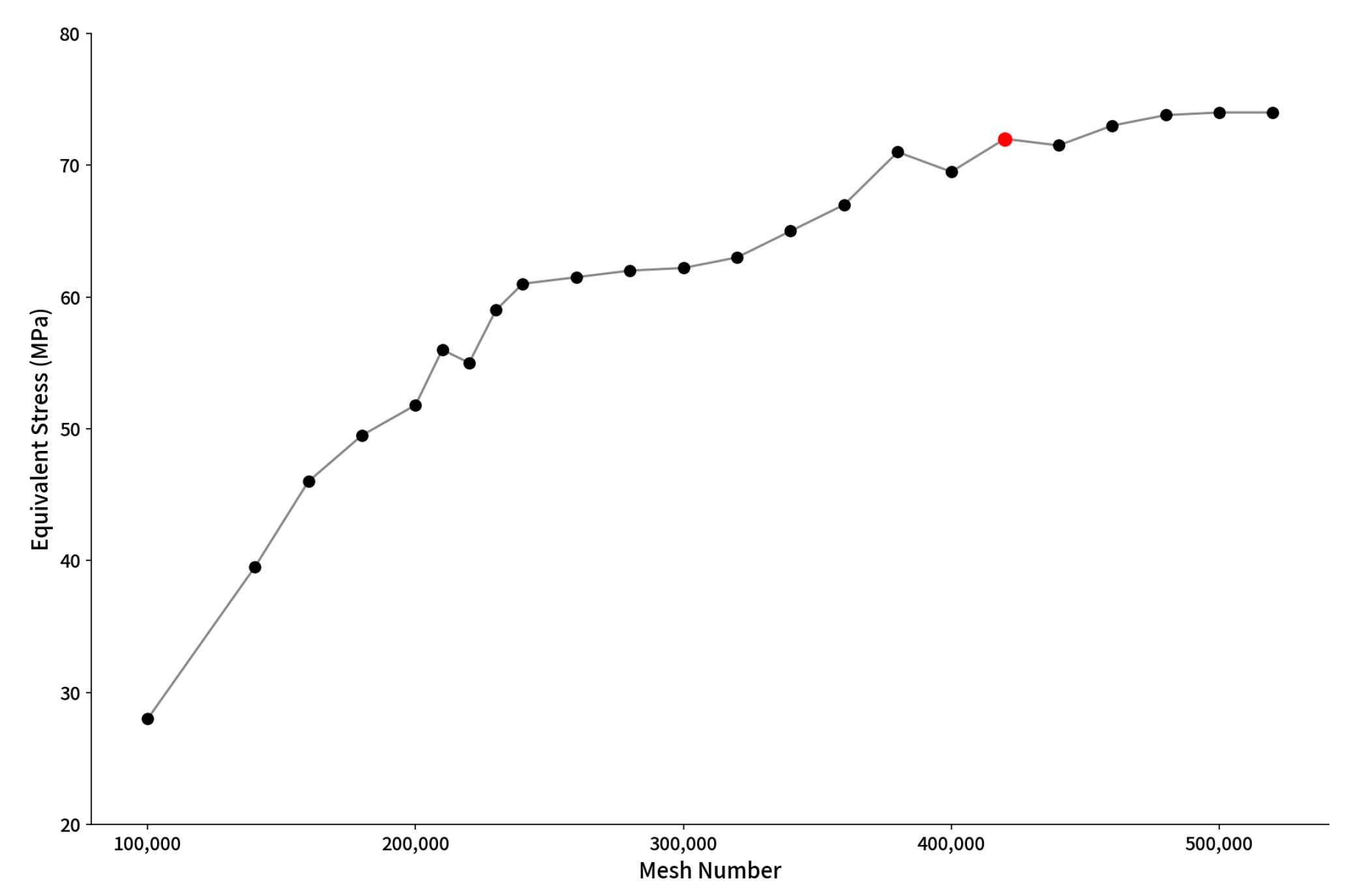
All 13 sets of 3D models of the support structures in their operational states were imported into Abaqus, and the models were meshed using a hexahedral mesh. Taking the model with a DN400 pipe and a connecting rod length of 190 mm as an example, the finite element mesh of the support structure is shown in Figure 9. Boundary conditions were set for the 13 support structures. Based on an analysis of the operating state of the infrared line drawing device, the support ear plate and support base were fully constrained to ensure that the threaded sleeve and rotating base remained fixed during operation. A uniformly distributed load was applied across the entire upper surface of the support plate; the resultant force of this load equaled the maximum compressive force exerted by the pipe inner wall on the support plate (736.605 N). Contact constraints were applied to the mating surfaces of the support ear plate, connecting rod, support plate, and support base, with a friction coefficient of 0.15. A mesh independence verification was performed. Figure 10 shows how the maximum equivalent stress on the support structure varies with the number of mesh elements. The mesh was refined until the relative change in the maximum stress between two consecutive mesh sizes was less than 2%. The calculation results began to stabilize when the number of mesh elements exceeded 430,000. To ensure accuracy while minimizing computational load, the final mesh element count was set to 439,117. At this point, the mesh quality check showed no warnings.

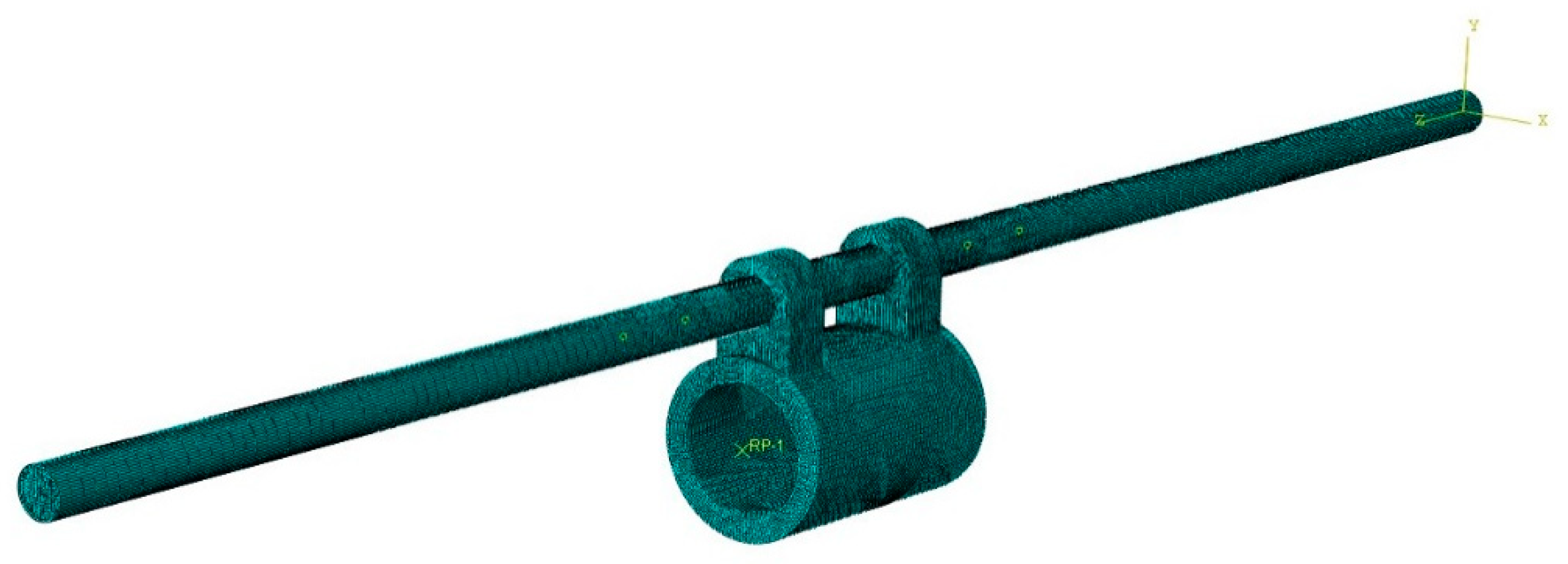
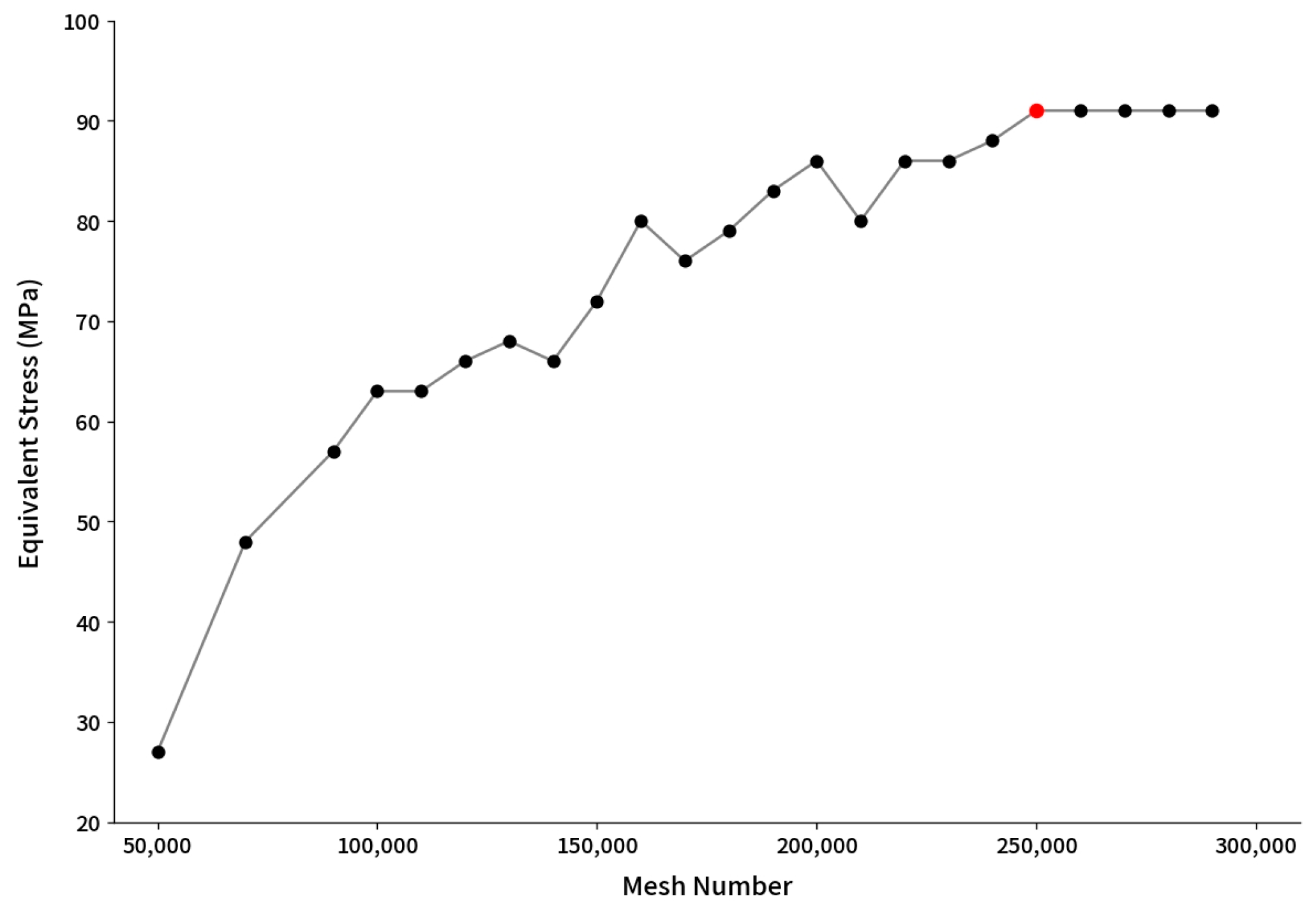
All 13 sets of 3D operational models of the guide structures were imported into Abaqus 2022 software, and the models were meshed using a hexahedral mesh. Taking the model with a DN400 pipe and a connecting rod length of 190 mm as an example, the finite element mesh model of the guide structure is shown in Figure 11. The boundary conditions for the 13 guide structures were set. Fully fixed constraints were applied to both ends of the guide rod component. A node named RP-1 was created at the center of the guide ear plate’s sleeve, and RP-1 was coupled to the guide ear plate to ensure synchronized motion. A rotational torque with a magnitude equal to the input torque M was applied to RP-1. A mesh independence verification was performed on the guide structure model. Figure 12 shows how the maximum equivalent stress on the guide structure varies with the number of mesh elements. The mesh was refined until the relative change in maximum stress between two consecutive mesh sizes was less than 2%. The calculation results began to stabilize when the number of mesh elements exceeded 230,000. To ensure accuracy while minimizing computational load, the final number of mesh elements for the guide structure was set to 239,553. At this point, the mesh quality check showed no warnings.

3.2. Finite Element Results

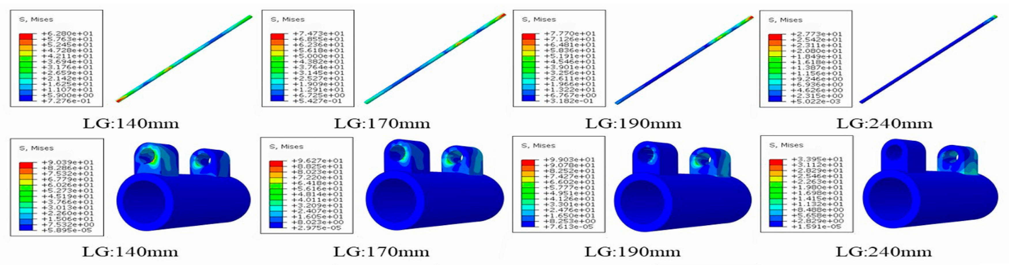
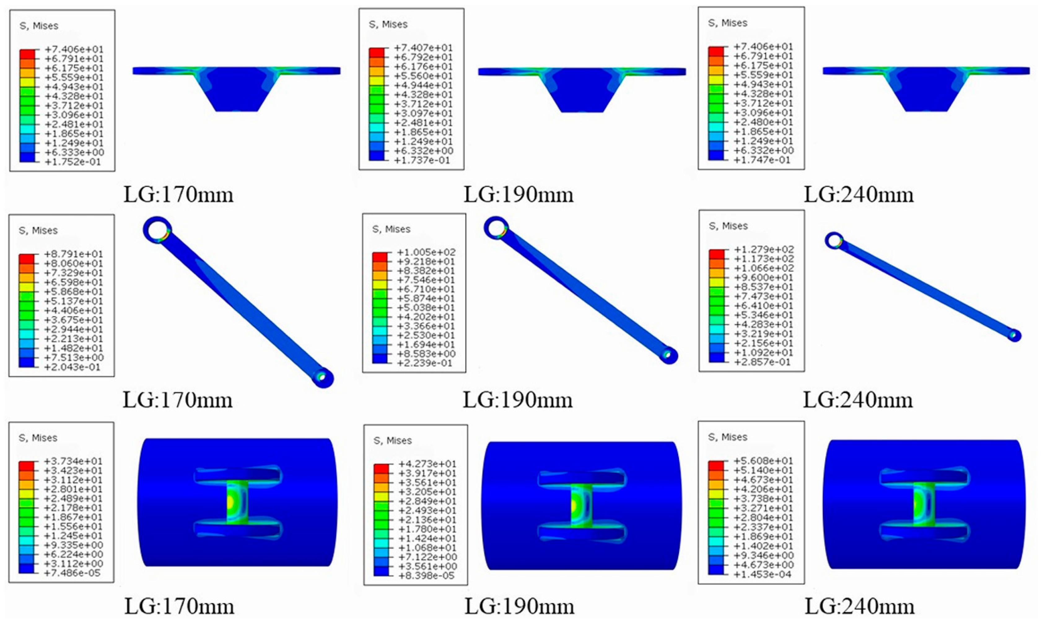
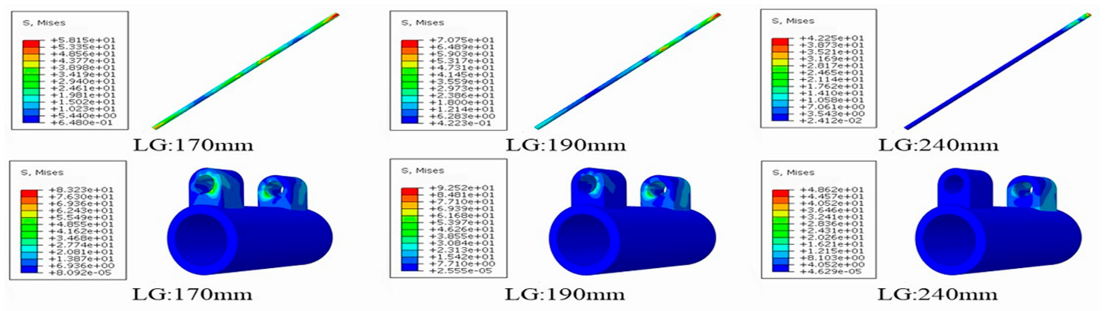
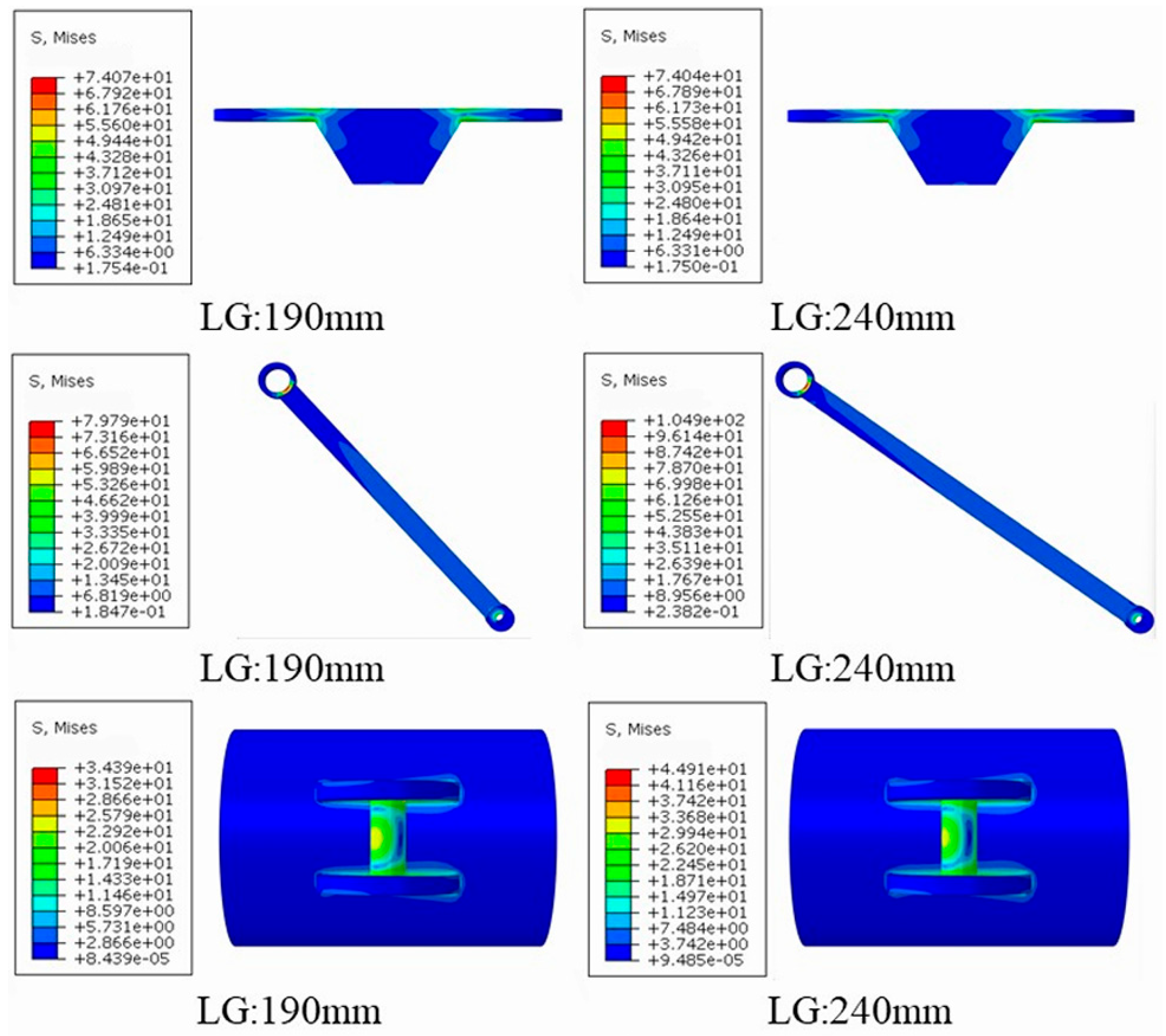
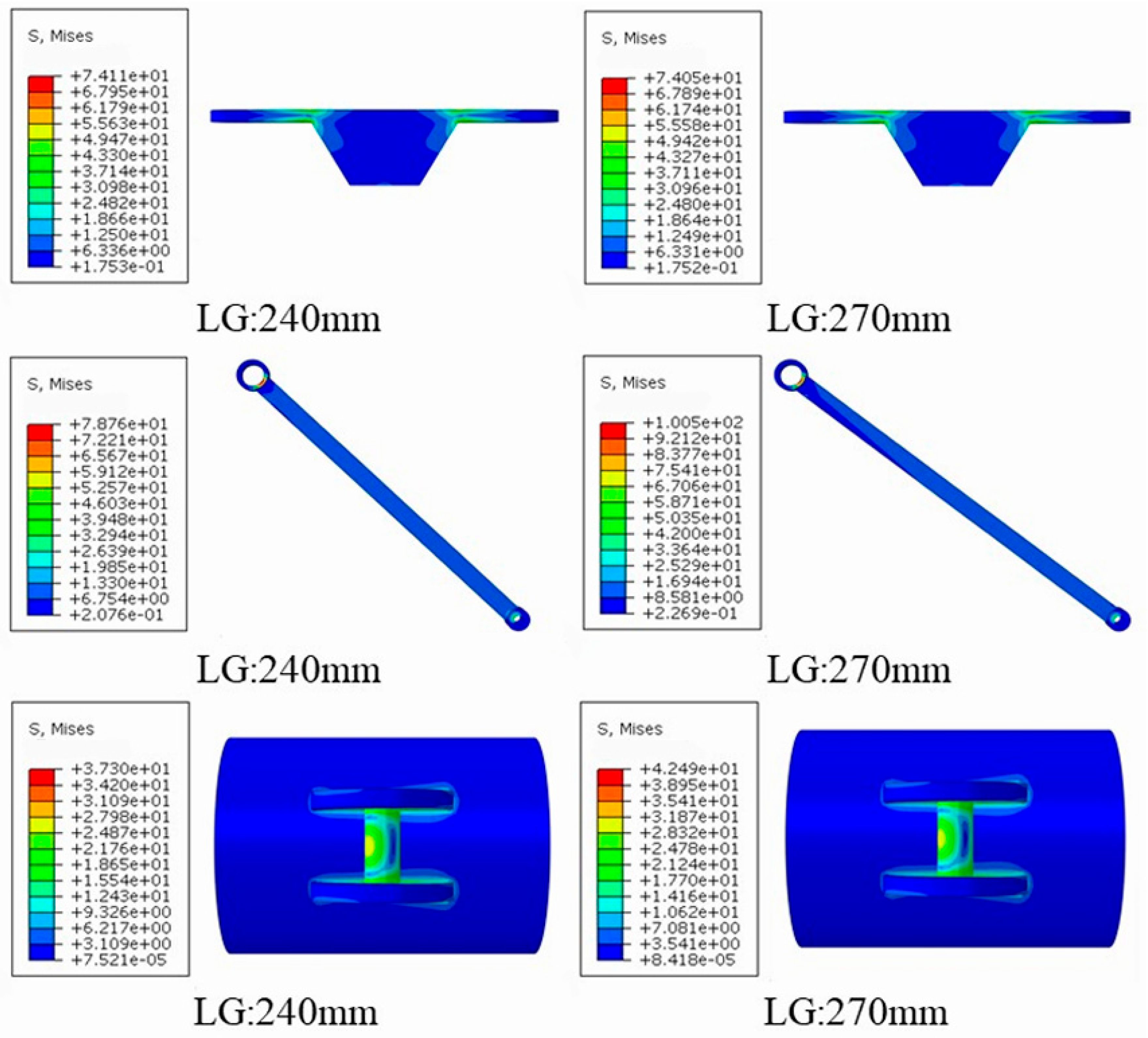
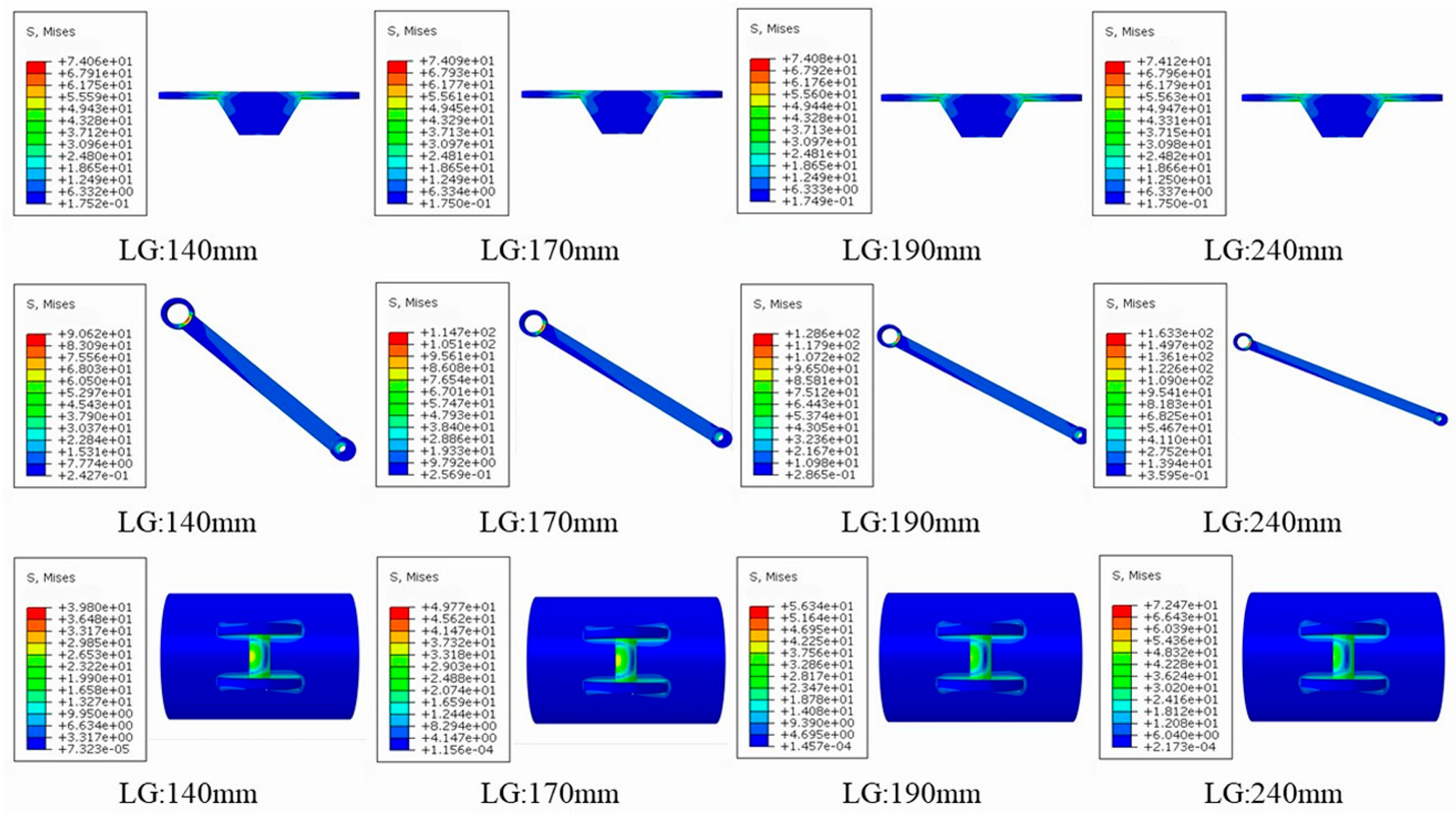
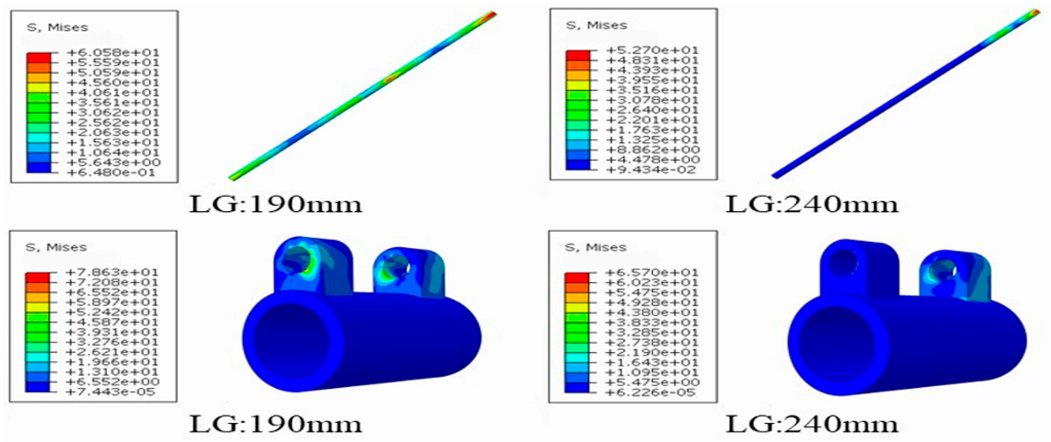
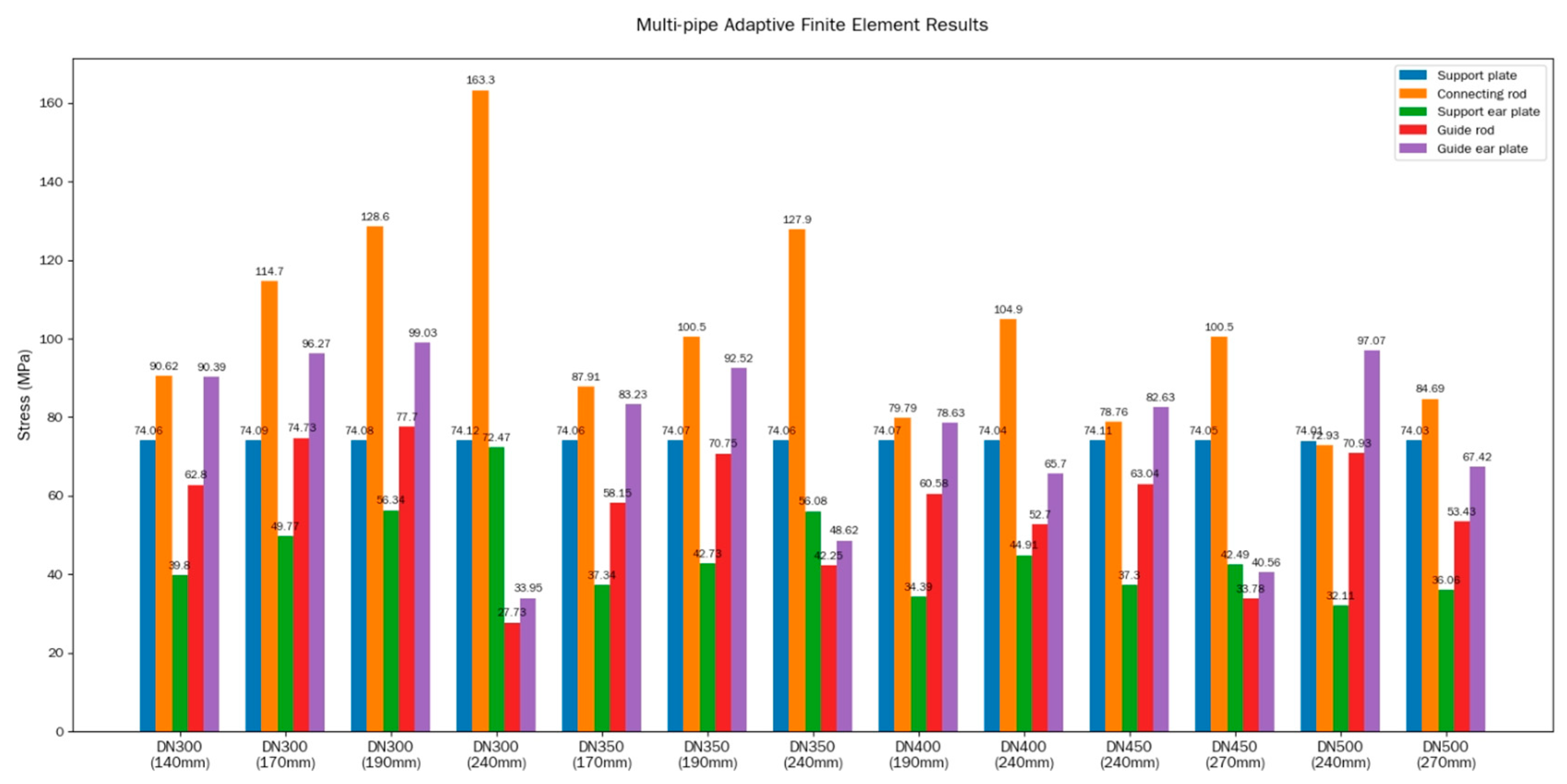
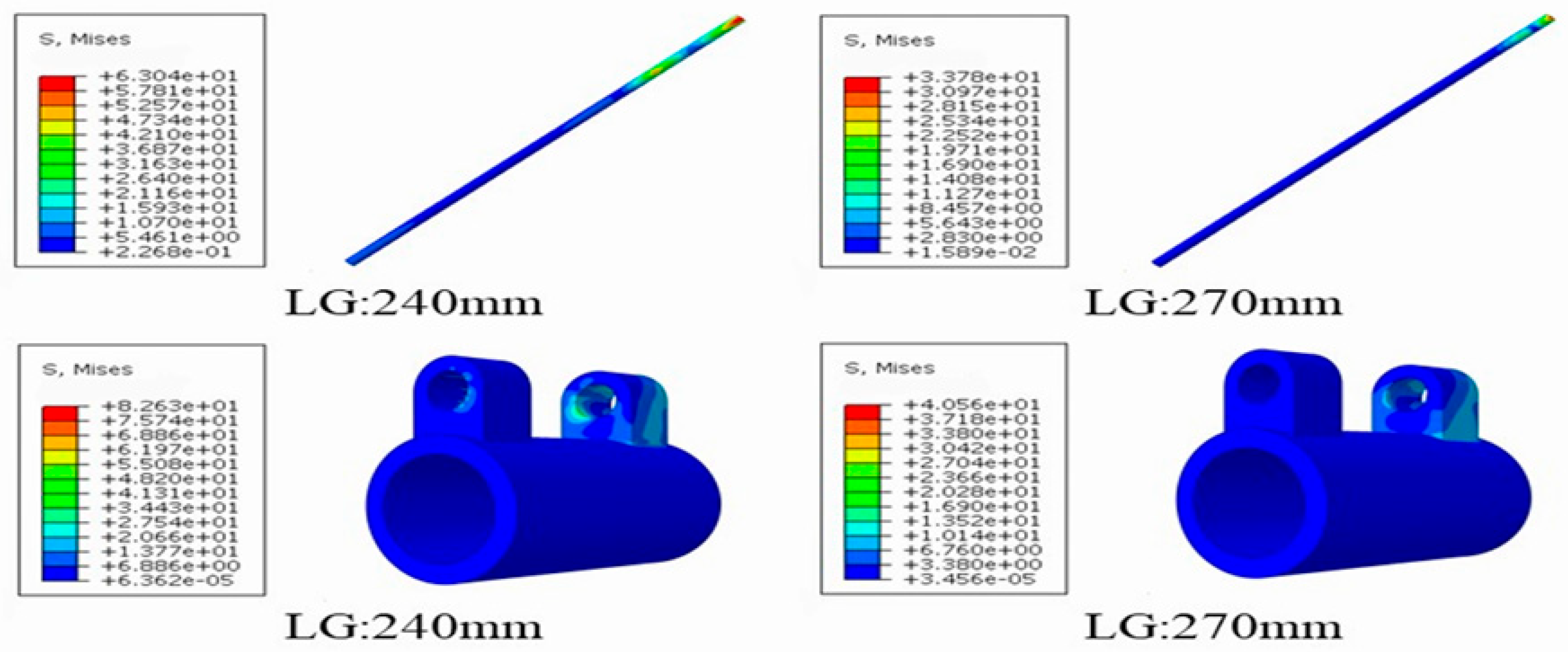
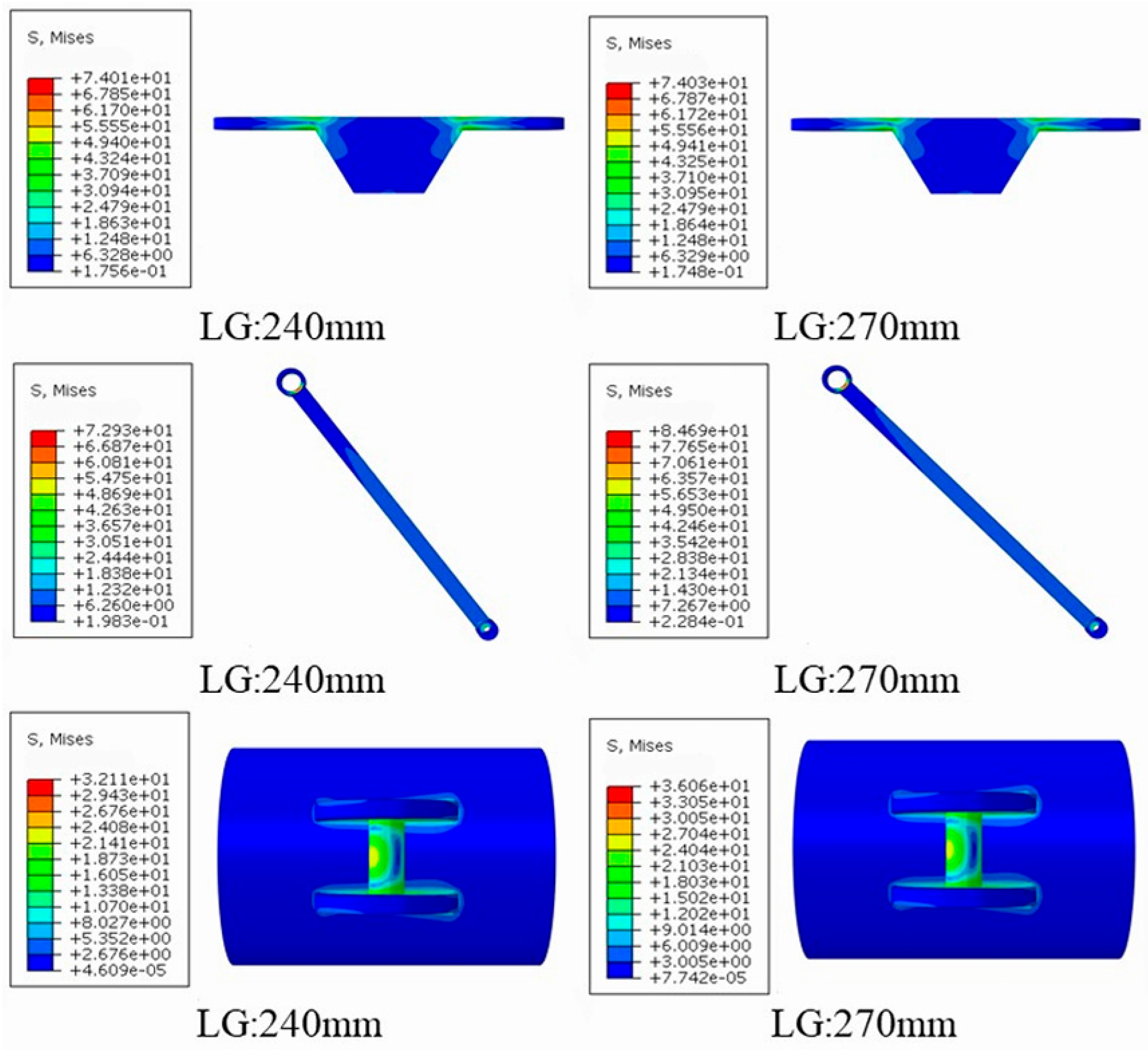
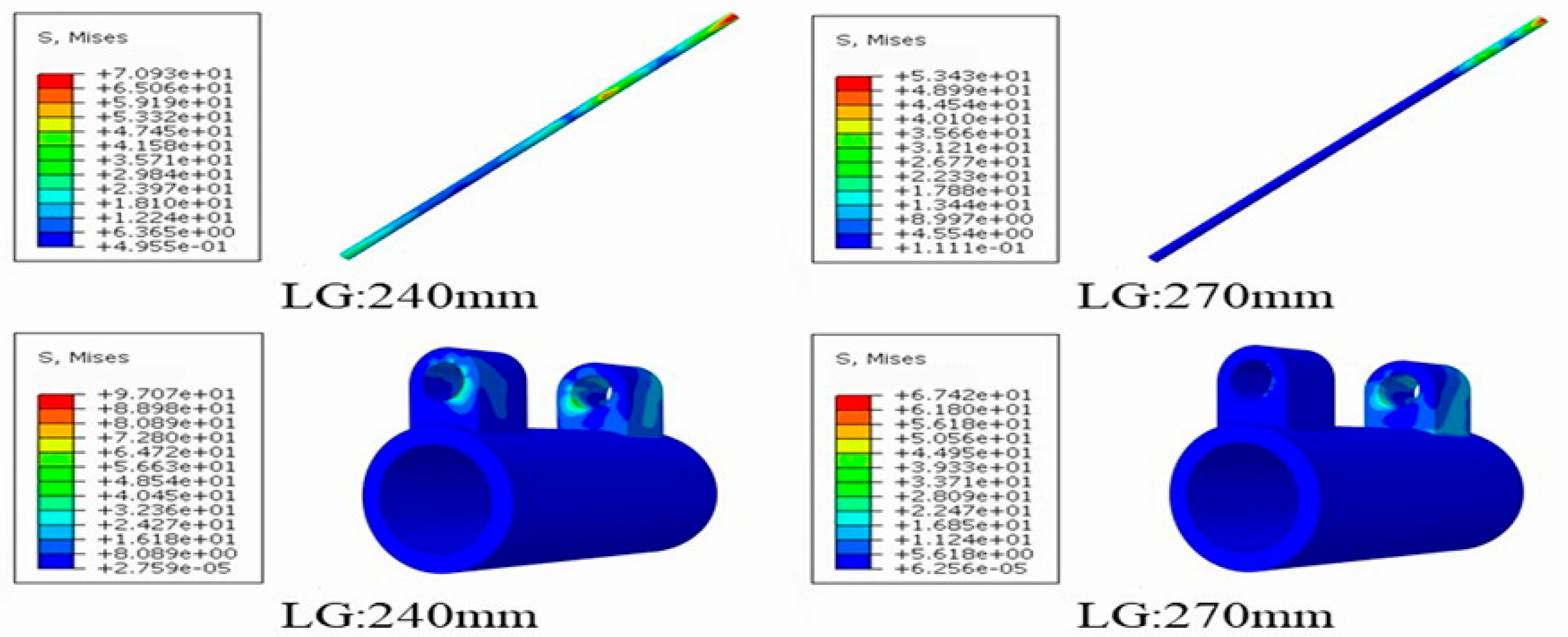
The equivalent stress distributions for all 13 operating conditions were obtained from the finite element simulations. Figure 13 presents a summary bar chart showing the maximum equivalent stress values for support plates, connecting rods, support ear plates, guide rods, and guide ear plates for each combination of pipe nominal diameter (DN300–DN500) and connecting rod length (140–270 mm). Detailed equivalent stress contour plots for all 13 operating conditions are provided in Appendix A (Figure A1, Figure A2, Figure A3, Figure A4, Figure A5, Figure A6, Figure A7, Figure A8, Figure A9 and Figure A10).

3.3. Analysis of Finite Element Results

Analysis shows that, under the 13 simulated operating conditions, the maximum equivalent stress of the key components remained within safe limits. To evaluate the stability of the operating conditions under each scenario, the variance of the stress data for the key components was calculated for each set of data, the results are shown in

Table 6. Summary table of multi-pipe adaptive variance data.

Nominal Diameter	140 mm	170 mm	190 mm	240 mm	270 mm
DN300	452.38	606.77	767.16	2930.32	—
DN350	—	425.51	502.82	1197.40	—
DN400	—	—	360.52	542.40	—
DN450	—	—	—	332.69	798.70
DN500	—	—	—	548.06	357.23

.

Based on the principle that the smaller the variance, the closer the service life of the components is to the ideal [32], the following conclusions are drawn.

(1)

For DN300 pipes, the optimal connecting rod length is 140 mm; for pipes ranging from DN300 to DN350, the optimal connecting rod length is 170 mm; for pipes ranging from DN300 to DN400, the optimal connecting rod length is 190 mm; for pipes ranging from DN300 to DN450, the optimal connecting rod length is 240 mm; for pipes ranging from DN300 to DN500, the optimal connecting rod length is 240 mm.

(2)

For DN350 pipes, the optimal connecting rod length is 170 mm; for pipes ranging from DN350 to DN400, the optimal connecting rod length is 190 mm; for pipes ranging from DN350 to DN450, the optimal connecting rod length is 240 mm; for pipes ranging from DN350 to DN500, the optimal connecting rod length is 240 mm.

(3)

For DN400 pipes, the optimal connecting rod length is 190 mm; for pipes ranging from DN400 to DN450, the optimal connecting rod length is 240 mm; for pipes ranging from DN400 to DN500, the optimal connecting rod length is 240 mm.

(4)

For DN450 pipes, the optimal connecting rod length is 240 mm.

(5)

For DN500 pipes, the optimal connecting rod length is 270 mm.

Since the variance data in Table 5 did not clearly identify the optimal connecting rod parameters for the DN450 to DN500 pipe range, variance calculations were further performed on the data for connecting rod lengths of 240 mm and 270 mm within this range. The results are shown in

Table 7. Summary table of variance of connecting rods for DN450~DN500 pipes.

Nominal Diameter	140 mm	170 mm	190 mm	240 mm	270 mm
DN450~DN500	—	—	—	392.84	520.28

. Based on these results, the optimal connecting rod parameter for the DN450 to DN500 pipe range was determined to be 240 mm.

The optimal link parameter values for pipelines of different diameters were compiled to create a table of optimal link parameter values for pipelines ranging from DN300 to DN500, as shown in

Table 8. Optimal parameters for connecting rods across the entire pipeline range.

DN	LG	DN	LG	DN	LG	DN	LG	DN	LG
300	140	350	170	400	190	450	240	500	270
~350	170	~400	190	~450	240	~500	240
~400	190	~450	240	~500	240
~450	240	~500	240
~500	240	“DN” represents the nominal diameter of the pipe. “LG” represents the optimal connecting rod length parameter.

. This table serves as a reference for on-site emergency repair personnel to quickly select the appropriate link parameters for infrared marking devices based on actual pipeline conditions.

4. Conclusions

(1)

The optimal length of the three mounting bolts for the centering deflection mechanism is 85 mm. At this length, the maximum deflection angle is 9.25°, and the mounting radius of 67.95 mm is less than or equal to the mounting plate radius of 93 mm, thereby meeting the axial alignment accuracy requirements for DN300 to DN500 pipes. The design of the marking mechanism indicates that when the deflection angle θ = 10°, the spring extension distance must be ≥4.1 mm. Based on this, the design parameters of a 5 mm marking pen tip length and a 5 mm spring extension are determined, which can effectively compensate for elliptical trajectory errors.

(2)

Based on 13 sets of finite element analysis and the principle of minimizing component stress variance, a parameter selection system for connecting rods across different bore diameters was established.

Single pipe diameter scenarios: DN300 (140 mm), DN350 (170 mm), DN400 (190 mm), DN450 (240 mm), DN500 (270 mm).

Combined pipe diameter scenarios: DN300–DN350 (170 mm), DN300–DN400 (190 mm), DN300–DN450 (240 mm), DN300–DN500 (240 mm), DN350–DN400 (190 mm), DN350–DN450 (240 mm), DN350–DN500 (240 mm), DN400–DN450 (240 mm), DN400–DN500 (240 mm), DN450–DN500 (240 mm). The 240 mm connecting rod can cover 75% of the range of pipe diameters.

Due to the limitations of research cycle, experimental site conditions and available equipment, the physical experimental platform and prototype verification are not included in the current work. Nevertheless, the established numerical model is reliable and rational based on theoretical derivation and literature comparison. Relevant experimental validation will be arranged in future research by constructing a dedicated experimental stand to further calibrate and optimize the proposed model.

References

- Hocine, A.; Achira, F.S.K.; Habbar, G.; Levent, A.; Medjdoub, S.M.; Maizia, A.; Dhaou, M.H.; Bezazi, A. Structural integrity assessment of corroded pipelines repaired with composite materials—Literature review. Int. J. Press. Vessel. Pip. 2024, 210, 105253. [Google Scholar] [CrossRef] [Scilit]
- Вoрoна, Г.В.; Махненкo, О.В.; Міленін, О.С. Effectiveness of Unloading a Section of Nps Pipeline with a Pipe Wall Thinning Defect by Mounting a Band or Welded Sleeve. Tech. Diagn. Nondestruct. Test-Ing. 2023, 11–19. [Google Scholar] [CrossRef] [Scilit]
- Kossenas, K.; Podilchak, S.K.; Beveridge, M. Wireless Propagation in a Metallic Pipe for the Transmission of Sensory Oil and Gas Well Data. IEEE Antennas Wirel. Propag. Lett. 2022, 21, 1124–1128. [Google Scholar] [CrossRef] [Scilit]
- Li, R.; Zhang, W.; Zhen, Z.; Jing, Y.; Bin, T.; Xu, S.; Manli, D.; Wang, Y. Discussion on repair technology of girth weld defects of high-grade steel pipelines. You-Qi Chuyun 2020, 39, 307–312. [Google Scholar]
- Kou, B.; Liu, E.; Li, D.; Qiao, W.; Chen, R.; Peng, S. Research on Erosion Characteristics of the Sleeve- Type Blowdown Valve in the Shale Gas Gathering and Transportation Station. SPE J. 2024, 29, 328–345. [Google Scholar] [CrossRef] [Scilit]
- Li, L.; Zhu, L.; Yan, X.; Jia, H.; Xie, S.; Zou, Y. The Impact of Weld Repairs on the Microstructure and Mechanical Integrity of X80 Pipelines in Oil and Gas Transmission. Processes 2025, 13, 512. [Google Scholar] [CrossRef] [Scilit]
- Dzhemilev, E.; Shammazov, I.; Sidorkin, D.; Arctic, S.C.; Mastobaev, B.; Gumerov, A. Developing technology and device for the main pipelines repair with cutting out their defective sections. Neft. Khozyaystvo-Oil Ind. 2022, 2022, 78–82. [Google Scholar] [CrossRef] [Scilit]
- Wasim, M.; Djukic, M.B. External corrosion of oil and gas pipelines: A review of failure mechanisms and predictive preventions. J. Nat. Gas Sci. Eng. 2022, 100, 104467. [Google Scholar] [CrossRef] [Scilit]
- Lam, C.; Zhou, W. Statistical analyses of incidents on onshore gas transmission pipelines based on PHMSA database. Int. J. Press. Vessel. Pip. 2016, 145, 29–40. [Google Scholar] [CrossRef] [Scilit]
- Ghaffari, R.; Javadian, N. Evaluating the Risk and Economic Implications of Pipeline Repair versus Replacement: A Case Study on Third-Party, Corrosion, and Design Issues. J. Pipeline Syst. Eng. Pract. 2026, 17, 05025009. [Google Scholar] [CrossRef] [Scilit]
- Adabavazeh, N.; Nikbakht, M.; Amindoust, A.; Hassanzadeh-Tabrizi, S.A. Assessing the reliability of natural gas pipeline system in the presence of corrosion using fuzzy fault tree. Ocean Eng. 2024, 311, 118943. [Google Scholar] [CrossRef] [Scilit]
- Shammazov, I.A.; Sidorkin, D.I.; Dzhemilev, E.R. Research of the Dependence of the Pipeline Ends Displacement Value When Cutting Out Its Defective Section on the Elastic Stresses in the Pipe Body. IOP Conf. Ser. Earth Environ. Sci. 2022, 988, 022077. [Google Scholar]
- Li, Y.; Liu, X.; Guo, J.; Li, Y.; Lu, Q.; Wang, M.; Sun, G.; Yu, J. Research on pipeline misalignment calculation method based on LCR wave stress detection results. Eng. Mech. 2025, 1–12. [Google Scholar] [CrossRef]
- Liu, E.-B.; Huang, S.; Tian, D.-C.; Shi, L.-M.; Peng, S.-B.; Zheng, H. Experimental and numerical simulation study on the erosion behavior of the elbow of gathering pipeline in shale gas field. Pet. Sci. 2024, 21, 1257–1274. [Google Scholar] [CrossRef] [Scilit]
- Li, Y.; Wang, L.; Jiang, Y.; Wang, S. Calculation method for cutting quantity of long-distance pipeline butt joint. Oil Gas Storage Transp. 2022, 41, 318–323. [Google Scholar] [CrossRef]
- Shammazov, I.; Dzhemilev, E.; Sidorkin, D. Improving the Method of Replacing the Defective Sections of Main Oil and Gas Pipelines Using Laser Scanning Data. Appl. Sci. 2023, 13, 48. [Google Scholar]
- Newman, N. Appropriate Methods for Repairing Pipelines. Pipeline Gas. J. 2020, 247, 41–42. [Google Scholar]
- Al-Douri, A.; Halim, S.Z.; Quddus, N.; Kazantzi, V.; El-Halwagi, M.M. A stochastic approach to evaluating the economic impact of disruptions in feedstock pipelines on downstream production. Process Saf. Environ. Prot. 2022, 162, 187–199. [Google Scholar]
- Yang, Z.; Zhang, L.; Zhang, J.; Zhao, Z.; Su, H.; Zio, E.; Faber, M.H. Flow structure: Identifying the essence of natural gas pipeline system resilience. Reliab. Eng. Syst. Saf. 2026, 266, 111631. [Google Scholar]
- Peng, S.; Zhang, Y.; Zhao, W.; Liu, E. Analysis of the Influence of Rectifier Blockage on the Metering Performance during Shale Gas Extraction. Energy Fuels 2021, 35, 2134–2143. [Google Scholar] [CrossRef] [Scilit]
- Aliyev, I. Engineering Solutions for Non-Stationary Gas Pipeline Reconstruction and Emergency Management. Int. J. Tech. Phys. Probl. Eng. 2024, 16, 181–193. [Google Scholar]
- Aliabadi, M.M.; Esmaeili, R.; Mohammadfam, I.; Ashrafi, M. Application of a Standardized Plant Analysis Risk-human Reliability Method to Pipeline Inspection Gauge Operations. J. Occup. Hyg. Eng. 2020, 3, 34–43. [Google Scholar]
- Bitelli, G.; Roncari, G.; Tini, M.A.; Vittuari, L. High-precision topographical methodology for determining height differences when crossing impassable areas. Measurement 2018, 118, 147–155. [Google Scholar] [CrossRef] [Scilit]
- Guo, R.; Hu, H.; Zhao, H.; Zhang, Y. Stress Concentration Factors Due to Misalignment at Girth Welds in Bi-Layer Pipes. J. Mar. Sci. Eng. 2024, 12, 231. [Google Scholar] [CrossRef] [Scilit]
- Liu, E.; Li, S.; Zhao, D.; Peng, S. Identification of acoustic spectral characteristics and propagation attenuation-based localization for gas pipeline leakage. Gas Sci. Eng. 2026, 145, 205801. [Google Scholar] [CrossRef] [Scilit]
- Chen, X.; Zhang, D.; Wang, X. Main problems and countermeasures of girth welds of oil and gas pipelines. You-Qi Chuyun 2021, 40, 1072–1080. [Google Scholar]
- Motta, L.; Novelli, P.; Darcis, P.; Armengol, M.; Tintori, F. Flowlines and Risers Pipes Ends Laser Measurement for Enhanced Girth Welds Manufacturing and Fatigue Behavior. In Proceedings of the ASME 2011 30th International Conference on Ocean, Offshore and Arctic Engineering, Rotterdam, The Netherlands, 19–24 June 2011. [Google Scholar]
- Bao, X.; Wang, M.; Zhou, H.; Guo, S. Non-contact laser-based method for measuring underground pipeline diameter. Yi Qi Yi Biao Xue Bao/Chin. J. Sci. Instrum. 2024, 45, 200–208. [Google Scholar]
- Sato, T.; Sato, Y.; Maekawa, T. Tool path generation for chamfering drill holes of a pipe with constant width. Comput.-Aided Des. 2016, 78, 26–35. [Google Scholar] [CrossRef] [Scilit]
- Tan, J.; Peng, S.; Liu, E. Spatio-temporal distribution and peak prediction of energy consumption and carbon emissions of residential buildings in China. Appl. Energy 2024, 376, 124330. [Google Scholar] [CrossRef] [Scilit]
- Xie, J.; Yang, G.; Qin, Y. Structural feature recognition and motion law simulation of dangerous rock mass based on UAV and Rockfall. J. Henan Polytech. Univ. Nat. Sci. 2021, 40, 55–64. [Google Scholar] [CrossRef]
- Zhang, F.; Zhao, Y.; Zhang, D.; Li, Y. Application of Variance Analysis Method in Aircraft Life-limiting Components Life Analysis. Aircr. Des. 2020, 40, 58–60. [Google Scholar] [CrossRef]
Figure 1.
Flowchart of the cutting process for corroded pipe. (a) Corroded pipeline segment; (b) Pipeline after removal of the corroded section via dead-end cutting; (c) Repaired pipeline with a new pipe spool installed.
Figure 2.
Overall structure of infrared line drawing device. (a) Support mechanism; (b) Centering deflection mechanism; (c) Marking mechanism; (d) Diagram of the operating states of the transmitter and receiver. 1 Trapezoidal threaded rod; 2 Threaded sleeve; 3 Connecting rod; 4 Support plate; 5 Housing; 6 Support mechanism; 7 Centering deflection mechanism; 8 Marking pen; 9 Marking bracket; 10 Laser emitter; 11 Laser pen; 12 Mounting plate; 13 Rotating ring; 14 Rotating plate; 15 Mounting bolt; 16 Pipeline; 17 The transmitting end; 18 Laser; 19 The receiving end; 20 Pipeline.
Figure 3.
Diagram of the centering deflection mechanism in operation.
Figure 4.
Simplified diagram of the planar layout.
Figure 5.
Simplified diagram of the three-bolt support configuration.
Figure 6.
Diagram of the marking mechanism in operation.
Figure 7.
Diagram of the internal structure parameters of a drawing pen.
Figure 8.
Support structure and guide structure model diagram.
Figure 9.
Finite element mesh model of the support structure.
Figure 10.
Verification of the mesh independence of the support structure.
Figure 11.
Finite element mesh model of the guide structure.
Figure 12.
Verification of the mesh independence of the guide structure.
Figure 13.
Multi-pipe adaptive finite element results.