Estimation of the Voltage Stability Margin in Power Systems Under Transmission Line Contingencies Using a Convex Formulation and a Heuristic Approach

Abstract

Voltage stability under transmission line contingencies is a critical concern in modern power systems, as the growing electricity demand and the large-scale integration of renewable energy sources increasingly challenge the security of network operation. This paper addresses the problem of estimating the voltage stability margin under $N-1$ transmission line contingencies through three solution methodologies: a nonlinear programming formulation solved via an interior-point algorithm (IPOPT) with a multi-start strategy, a recursive heuristic approach based on successive Newton–Raphson power flow solutions with progressive load scaling, and a convex second-order cone programming relaxation. The proposed methods are validated on the IEEE 9-, 14-, 30-, and 57-bus test systems, thereby covering networks of varying topological complexity and redundancy. A comparative analysis evaluates the accuracy of each approach against a nonlinear programming reference, as well as their computational efficiency under a comprehensive set of contingency scenarios. The results indicate that the heuristic method achieves higher precision, while the convex formulation offers a substantially faster solution, with both approaches demonstrating robustness in cases where the nonlinear programming method fails to converge.

1. Introduction

The rapid growth in the electricity demand is a direct consequence of technological advancement and the increasing electrification of strategic sectors. According to the International Energy Agency, the global electricity demand rose by $4.3\%$ in 2024, compared to $2.3\%$ in 2023 [1], reflecting a significant acceleration relative to previous years and, consequently, imposing new challenges on existing electrical infrastructure. In parallel, the energy transition being pursued by numerous countries, with the aim of meeting the Sustainable Development Goals and the targets set by the Paris Agreement, has driven the large-scale integration of non-conventional renewable energy sources and the widespread adoption of distributed generation (DG) [2,3]. These developments are fundamentally transforming the traditional operation of power systems [4].

As a result of these structural changes, the inherent variability of renewable generation, coupled with the reduction in system inertia that is typically provided by synchronous generators, increases the vulnerability of power systems to contingencies, with a particularly pronounced effect on voltage stability [5]. This loss of stability can trigger a progressive and uncontrollable decline in voltage, potentially leading to collapse [6]. Such an event may entail cascading failures and large-scale blackouts, leading to severe economic and social consequences. In particular, unplanned transmission line outages represent one of the most critical threats to maintaining a secure voltage profile [7]. Thus, the reliability of transmission subsystems and the occurrence of line contingencies are key aspects in the safe operation of power systems [8]. In this context, estimating the voltage stability margin becomes an essential tool for both the planning and preventive operation of electrical networks.

Numerous academic studies have addressed this problem from various perspectives. For instance, Ref. [9] analyzed voltage stability using the Jacobian power flow matrix, noting that, at the maximum loadability point, this matrix becomes singular, indicating proximity to voltage collapse. To accurately determine this point, the continuation power flow method is commonly employed, which introduces an additional parameter $\lambda$ to maintain convergence, even at the maximum loading point, and allows tracing the P-V curve beyond the collapse point. Other works have examined the impact of renewable generation on voltage stability, emphasizing the reduced inertia and intermittency associated with technologies such as wind power [10]. Furthermore, methodologies based on sensitivity analysis, dynamic monitoring, and contingency assessment have been proposed to identify critical operating conditions [11,12].

Recent years have seen a growing trend towards the use of optimization techniques for enhancing voltage stability margins. On the one hand, convex approaches—including semidefinite and second-order cone programming—allow finding globally optimal solutions with high computational efficiency [13,14,15,16]. On the other hand, heuristic and metaheuristic methods, such as particle swarm optimization (PSO), differential evolution, the second generation of the non-sorted genetic algorithm, and simulated annealing (SA), have proven effective in exploring the solution space and optimizing the placement of reactive power compensation devices or the implementation of power dispatch strategies [17,18,19]. In addition, the deployment of flexible AC transmission systems and high-voltage direct-current (DC) links has been shown to significantly improve voltage stability margins [20]. Modern computational tools such as PowerModels have further facilitated the implementation and benchmarking of various power flow formulations, promoting reproducibility and allowing for advanced stability analyses in large-scale systems [21].

Within this framework, our work seeks to estimate the voltage stability margin of electric power systems operating under transmission line contingencies. To this effect, different solution methodologies are introduced which combine a convex reformulation of the power flow problem using second-order cone programming; a nonlinear optimization formulation solved via the interior-point optimizer (IPOPT), an open-source software package designed for large-scale nonlinear optimization problems [22]; and a heuristic approach based on successive power flow solutions via the Newton–Raphson method. The proposed strategy capitalizes on the mathematical robustness inherent to convex formulations while retaining the adaptability of conventional iterative techniques for the detailed characterization of system behavior across a range of contingency scenarios. Our validations include standard IEEE test systems widely used in academic power system studies. Specifically, systems with 9, 14, 30, and 57 buses are employed, allowing for an assessment of the method’s performance across networks with varying levels of topological complexity.

The remainder of this paper is organized as follows. Section 2 presents the mathematical formulation of the voltage stability margin estimation problem under transmission line contingencies. Section 3 describes the proposed methodology, detailing the convex formulation and the heuristic approach. Section 4 outlines the test systems used in this study. Section 5 presents and discusses the results obtained for the different scenarios under analysis, and, finally, Section 6 presents the conclusions of this work and suggests potential directions for future research.

2. Mathematical Modeling

Voltage stability is a critical aspect of power system security. It has to do with the ability to sustain acceptable steady-state voltage magnitudes in all buses after a disturbance. In the context of transmission line contingencies, the sudden loss of a line can lead to significant voltage drops that may violate the operating limits and, if not properly managed, escalate to voltage collapse. Therefore, characterizing the maximum loadability limit of the system under such conditions is of paramount importance for both planning and operational purposes.

Definition 1 (Voltage stability and loadability factor).

Voltage stability is defined as a power system’s capacity to maintain acceptable voltage levels across all its buses following a disturbance  [1]. During contingencies such as transmission line outages, the voltage may drop below the established operating limits, thereby compromising the secure operation of the system [7]. In this context, the loadability factor λ quantifies the maximum proportional increase that can be simultaneously applied to active and reactive power demands without violating operational constraints or compromising power flow convergence [14,23].

2.1. Objective Function

Considering the above, the voltage stability margin estimation problem is formulated as a nonlinear optimization model based on the alternating-current (AC) power flow equations for contingency analysis [24], whose objective is to maximize the loadability coefficient $\lambda$. Let $\mathcal{C}=\{1,2,\dots ,n_l\}$ be the set of $N-1$ contingencies, where each element $c\in \mathcal{C}$ corresponds to the outage of a transmission line and $n_l$ denotes the total number of lines in the system. For each contingency c, the nodal admittance matrix ${\mathbf{Y}}_{\mathrm{bus}}^c$ is obtained by removing line c from the base system. For each line-related contingency, the maximum value of $\lambda$ quantifies the maximum simultaneous increase in active and reactive power demand that the system can accommodate without experiencing voltage collapse.

$$\lambda =min\left\{\underset{{\lambda }_c,V_i^c,{\theta }_i^c,P_{gi}^c,Q_{gi}^c}{max}{\lambda }_c\right\}$$

(1)

where $V_i^c$ represents the voltage magnitude at bus i, ${\theta }_i^c$ denotes the voltage angle at bus i, $P_{gi}^c$ and $Q_{gi}^c$ represent the active and reactive power injections at bus i, respectively, and ${\lambda }_c$ represents the maximum loadability margin under contingency c.

Remark 1.

It should be noted that the primary objective of solving (1) is to determine the minimum loadability factor of the power system by evaluating all possible transmission line contingencies, thereby identifying the most critical operating scenario.

2.2. Constraints

The optimization problem formulated in Equation (1) is subject to a set of operational and physical constraints that ensure a feasible operation of the power system under contingency conditions. These constraints include the active and reactive power balance equations at each bus, which govern the steady-state behavior of the network. The power balance equations, which incorporate the loadability factor $\lambda$ as a uniform scaling parameter applied to both active and reactive power demands, are expressed as follows.

Active power balance:

$$P_{gi}^c-{\lambda }^c{P}_{di}=V_i^c\sum _{j\in \mathcal{N}}{V}_j^c\left(G_{ij}cos{\theta }_{ij}+B_{ij}^{c}sin{\theta }_{ij}^c\right),\forall i\in \mathcal{N},\forall c\in \mathcal{C}$$

(2)

Reactive power balance:

$$Q_{gi}^c-{\lambda }^c{Q}_{di}=V_i^c\sum _{j\in \mathcal{N}}{V}_j\left(G_{ij}sin{\theta }_{ij}^c-B_{ij}cos{\theta }_{ij}^c\right),\forall i\in \mathcal{N},\forall c\in \mathcal{C}$$

(3)

Loadability factor:

$${\lambda }^c\ge 1,\forall c\in \mathcal{C},$$

(4)

where $\mathcal{N}$ denotes the set of buses in the system, and $G_{ij}$ and $B_{ij}$ represent the conductance and susceptance of branch $ij$ under contingency c. The limits $V_i^{min}$ and $V_i^{max}$ correspond to the minimum and maximum allowable voltage magnitudes, respectively, as specified in the corresponding MATPOWER data matrix.

The nonlinear and nonconvex nature of Equations (2) and (3) defines a nonlinear programming (NLP) problem that becomes computationally demanding for exact solution methods in large-scale systems [11]. This complexity motivates the development of the two solution approaches described in Section 3: a heuristic method and a convex method.

Remark 2.

The optimization model defined from (1) to (4) is formulated under the conventional assumptions of the AC power flow problem. Specifically, the voltage magnitude and angle are fixed at the slack bus, the voltage magnitude and active power injection are specified at the voltage-controlled buses (i.e., PV buses), and the active and reactive power demands are specified at the load buses (PQ buses).

3. Methodology

To solve the problem defined in Equations (1)–(4), this work proposes two solution approaches and compares them against a reference method that formulates the loadability problem as a NLP model which maximizes the loading factor $\lambda$ subject to the full AC power flow equations, solved using an interior-point algorithm. This serves as the baseline for comparative purposes.

The first approach estimates ${\lambda }_c$ through a recursive heuristic procedure that relies on successive AC power flow solutions via the Newton–Raphson method, with fixed load steps until divergence occurs. The second approach formulates the solution through a conic relaxation. Each method is applied independently to every contingency.

3.1. Reference Nonlinear Programming Model

This approach addresses the nonlinear problem defined in (1)–(4) using an interior-point algorithm that is implemented through the IPOPT solver. Although IPOPT does not guarantee a globally optimal solution, it enables the efficient exploration of large-scale and highly nonlinear problems such as the one studied herein, with a reduced computational burden [25]. Unlike continuation-based methods, this approach does not require the explicit construction of the Jacobian matrix nor the manual increment of the loading parameter $\lambda$. Instead, the optimizer directly determines the maximum value of $\lambda$ that satisfies all model constraints.

The solution obtained with IPOPT may correspond to a local optimum depending on the initialization point. To mitigate premature convergence, a multi-start strategy is employed, whereby the problem is solved repeatedly from $n_s$ distinct initial values of the voltage magnitude $V_0\in {\mathcal{V}}_s$. Similar strategies have been adopted in other optimization methods, such as variants of PSO that modify their search parameters to improve solution quality [26]. In this work, the set of initial conditions is defined as follows:

$${\mathcal{V}}_s=\{0.75,0.85,0.95,1.00,1.05\}\mathrm{p}.\mathrm{u}.$$

(5)

The value of ${\lambda }_c$ is then obtained as the maximum among all feasible solutions identified through the procedure defined in Algorithm 1.

Algorithm 1 Estimation of ${\lambda }_c$ using NLP with interior-point method and multi-start strategy.

Require: Base case, set of active lines $\mathcal{L}$, initial points ${\mathcal{V}}_s$ Ensure: ${\lambda }_c$ for each contingency $c\in \mathcal{L}$   1: for each line $c\in \mathcal{L}$ do   2:       Deactivate line c in the system and recompute the admittance matrix ${\mathbf{Y}}_{\mathrm{bus}}^c$   3:       Initialize the best loadability factor: ${\lambda }_c\leftarrow \mathtt{NaN}$   4:       for each starting point $v_0\in {\mathcal{V}}_s$ do   5:             Formulate the NLP problem: $$\underset{\lambda ,\mathbf{V},{\mathbf{S}}_g}{max}\lambda$$   6:             subject to: $$\begin{array}{c}{\overline{S}}_{g,k}-\lambda {\overline{S}}_{d,k}={\overline{V}}_k{\displaystyle \sum _{m=1}^N}{Y}_{km}^c{V}_m,\forall k\in \mathcal{N}\hfill \\ V_k=V_k^0,\forall k\in {\mathcal{N}}_{\mathrm{slack}}\hfill \\ |V_k{|}^2={\left(V_k^0\right)}^2,P_{g,k}=P_{g,k}^0,\forall k\in {\mathcal{N}}_{PV}\hfill \\ S_{g,k}=0,\forall k\in {\mathcal{N}}_{PQ}\hfill \\ \lambda \ge 1\hfill \end{array}$$   7:             Initialize all bus voltages as $V_k\leftarrow v_0$   8:             Solve the problem using the IPOPT solver   9:             if a feasible solution is found then 10:                  Store the obtained value of $\lambda$ 11:                  if this value of $\lambda$ exceeds the current ${\lambda }_c$ then 12:                        Update: ${\lambda }_c\leftarrow \lambda$ obtained from this initialization 13:                  end if 14:             else 15:                  Discard this starting point and proceed to the next 16:             end if 17:       end for 18:       Record ${\lambda }_c$ as the voltage stability margin for contingency c 19: end for   return Results table $\left\{{\lambda }_c\right\}$ for all $c\in \mathcal{L}$

This algorithm enables the systematic and robust estimation of the voltage stability margin under transmission line contingencies. Its mechanism, based on the repeated solution of the nonlinear optimization problem using the IPOPT solver, allows determining the maximum loadability factor that the system can support after the outage of each line.

Furthermore, the multi-start strategy, initialized under five distinct voltage conditions, mitigates the impact of convergence to local optima. Its implementation in Julia simplifies the configuration of different contingency scenarios and the integration of various test systems in MATPOWER format. Consequently, this combination enhances the reliability of the obtained solution and extends the applicability of the method to larger-scale power systems.

Remark 3.

From an implementation perspective, the proposed approach leverages the flexibility of high-level modeling environments to efficiently handle multiple contingency scenarios. In particular, the use of Julia in combination with optimization frameworks (e.g., JuMP) and the IPOPT solver facilitates the automated formulation and solution of the NLP model for each contingency. The multi-start strategy reinitializes the voltage magnitudes across a predefined set of starting points, ensuring a broader exploration of the feasible solution space while reducing sensitivity to initialization. This modular structure allows for a straightforward adaptation to different network sizes and data sources, including MATPOWER-based test systems.

3.2. Recursive Heuristic Approach

The continuous method estimates the loadability factor ${\lambda }_c$ through successive evaluations of the AC power flow, progressively increasing the system demand in fixed steps ($\Delta \lambda =0.001$), starting from the base operating condition $\lambda =1$ up to a maximum value of $\lambda =5$. At each step, the active and reactive power demands at all buses are proportionally scaled as follows:

$$P_{di}\left(\lambda \right)=\lambda P_{di}^0,Q_{di}\left(\lambda \right)=\lambda Q_{di}^0,\forall i\in \mathcal{N}$$

(6)

where $P_{di}^0$ and $Q_{di}^0$ correspond to the active and reactive power demands under baseline conditions.

For each value of $\lambda$, the AC power flow is solved using the Newton–Raphson method [27], whose iterative process updates the voltage magnitudes and angles at each bus. The increment in $\lambda$ is repeated until the Newton–Raphson method fails to converge at the current step, indicating that the system has reached its maximum loadability point [28].

The voltage stability margin for a given contingency is then approximated as the last value of $\lambda$ for which the power flow solution converged:

$${\lambda }_c\approx {\lambda }^{(t-1)}.$$

(7)

In (7), ${\lambda }^{(t-1)}$ denotes the last convergent value, and t represents the iteration at which divergence is detected. Algorithm 2 summarizes the proposed procedure.

Algorithm 2 Heuristic approach for the estimation of ${\lambda }_c$ using the Newton–Raphson method.

Require: Base case, contingency c, step size $\Delta \lambda =0.001$, ${\lambda }_{max}=5$ Ensure:  ${\lambda }_c$ 1: Remove line c from ${\mathbf{Y}}_{\mathrm{bus}}$ to obtain ${\mathbf{Y}}_{\mathrm{bus}}^c$ 2: Initialize $\lambda \leftarrow 1$ 3: repeat 4:       $\lambda \leftarrow \lambda +\Delta \lambda$ 5:       Scale demands according to (6) 6:       Solve the AC power flow using the Newton-Raphson method 7: until NR fails to converge or $\lambda >{\lambda }_{max}$ 8: ${\lambda }_c\leftarrow \lambda -\Delta \lambda$  return  ${\lambda }_c$

3.3. Second-Order Cone Approximation

In this approach, the problem is formulated as a convex quadratic optimization program defined over squared voltage magnitudes $Z_k={\left|V_k\right|}^2$ and pairwise voltage products $W_{km}=V_k{V}_m^{\ast }$ [14]. The main constraints are described as follows:

• Nodal voltages. For slack and PV buses, the voltage magnitudes are fixed as follows:

  $$\begin{array}{c}\hfill Z_k={\left|V_k^0\right|}^2,\forall k\in {\mathcal{N}}_{\mathrm{slack}}\cup {\mathcal{N}}_{PV}.\end{array}$$

  (8)
• Power balance. The net power injection at each bus is expressed in terms of W through the network admittance matrix:

  $$\begin{array}{c}\hfill S_{g,k}-\lambda S_{d,k}={\displaystyle \sum _{m=1}^N}{Y}_{km}{W}_{km},\forall k\in \mathcal{N}.\end{array}$$

  (9)
• Voltage relationships between buses. Convex constraints ensure a second-order cone representation:

  $$\begin{array}{c}\hfill 4|W_{km}{|}^2+|Z_k-Z_m{|}^2\le {|Z_k+Z_m|}^2,\forall (k,m)\in \mathcal{L}.\end{array}$$

  (10)
• Generation constraints. For the PQ buses, $S_{g,k}=0$ is enforced; for the PV buses, the active power is fixed as:

  $$\begin{array}{c}\hfill P_{g,k}=P_{g,k}^0,\forall k\in \mathcal{N}.\end{array}$$

  (11)
• Loading factor. The objective is to maximize $\lambda$:

  $$\begin{array}{c}\hfill max\lambda \mathrm{subject}\mathrm{to}\mathrm{the}\mathrm{above}\mathrm{constraints}.\end{array}$$

  (12)

The convex relaxation is exact—i.e., it recovers the true AC power flow solution—under sufficient conditions, as is the case with radial (tree) networks with no upper bounds on voltage angles [29]. For meshed transmission systems, however, the relaxation may not be globally exact. In such cases, the SOCP (Second-Order Cone Programming) formulation provides a lower bound on the true loadability margin ${\lambda }_c$ (optimistic estimate), meaning that it may overestimate the actual voltage stability limit. Conversely, the NLP reference method solves the original non-convex problem but may converge to a local optimum, potentially underestimating ${\lambda }_c$. Therefore, comparing both methods reveals not only their accuracy but also the presence and magnitude of any relaxation gap.

From a numerical and engineering perspective, the convex approximation is sufficiently accurate to locate the voltage collapse region, even when the relaxation is not perfectly tight. The convex estimate consistently identifies the critical contingency (i.e., the line whose removal causes the greatest reduction in $\lambda$) and provides an approximate loading margin at which collapse occurs. Small relaxation gaps (e.g., <5%) do not alter the ranking of contingencies nor the practical assessment of system vulnerability. For online contingency screening, where speed and robustness are paramount, the convex method offers a reliable indicator of the collapse point location, with errors well within typical operational safety margins [30].

In our numerical results, the reported relaxation gaps (i.e., the difference between the convex lower bound and the local NLP solution) remain below $2\%$ for most test cases [14]. However, when the gap exceeds a predefined threshold (e.g., >5%), the convex estimate should be interpreted as an optimistic bound, requiring either a tightening procedure (e.g., adding valid inequalities) or a post-processing recovery step to reconstruct a feasible AC solution. For absolute accuracy regarding a specific critical contingency, the convex solution can be refined via a local NLP step.

The implementation of the SOCP approach for line contingency analysis is presented in Algorithm 3.

Algorithm 3 Estimation of ${\lambda }_c$ using convex relaxation.

Require: Base case, set of active lines $\mathcal{L}$ Ensure: ${\lambda }_c$ for each contingency $c\in \mathcal{L}$   1: for each line $c\in \mathcal{L}$ do   2:       Deactivate line c and recompute ${\mathbf{Y}}_{\mathrm{bus}}^c$   3:    Formulate the convex problem using variables $Z_k$ and $W_{km}$   4:       Enforce voltage, power balance, and SOC constraints   5:       Solve via a convex solver (e.g., Clarabel)   6:       if a feasible solution is found then   7:             Store $\lambda$ as ${\lambda }_c$   8:       else   9:             Record infeasibility (collapse before first step) 10:       end if 11: end for    return $\left\{{\lambda }_c\right\}$ for all contingencies

The convex approach ensures global optimality within its feasible set, reduces sensitivity to initialization, and enables an efficient contingency evaluation. For online deployment, the authors recommend computing the relaxation gap by solving a small feasibility problem that reconstructs voltage angles from $W_{km}$. If the gap is significant, the result should be flagged for further analysis or complemented with a local NLP refinement.

Remark 4.

From an implementation standpoint, the convex formulation can be efficiently handled using JuMP in Julia with solvers like Clarabel. A practical strategy to assess relaxation tightness is to recover the voltage angles ${\theta }_k$ from $W_{km}$ via ${\theta }_k-{\theta }_m=arg\left(W_{km}\right)$ and check whether these angles satisfy the original AC power balance within a small tolerance range (e.g., $1\%$). If the violation exceeds this threshold, the relaxation is not exact, and the estimated ${\lambda }_c$ should be regarded as an optimistic bound—nonetheless, its value remains sufficient to locate the region of voltage collapse for engineering decision-making.

4. Test Systems

The proposed methodology was evaluated using standard IEEE test systems, with data obtained from the MATPOWER library, a widely used tool in academic and research studies on electric power systems [31]. Specifically, the IEEE 9-, 14-, 30-, and 57-bus test cases were considered. Electrical parameters, including line impedances, charging susceptances, generator data, and load profiles, are available in the following repository: Test Systems (https://github.com/mafe1328/StabilityAnalysisCases.git, accessed on 13 March 2026).

4.1. The IEEE 9-Bus System

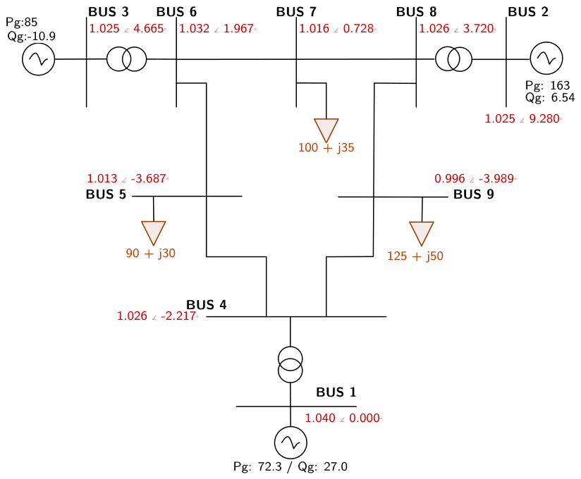
This system represents a classic three-machine, nine-bus power network, as depicted in Figure 1. Widely used as a benchmark for transient stability, small-signal stability, and controller design [32], it features three synchronous generators, three loads, and nine transmission lines arranged in a meshed topology. The generators are located at buses 1 (slack), 2, and 3, each equipped with a standard exciter and governor. The loads total approximately 315 MW and 115 Mvar. Despite its moderate size, the system captures essential dynamic phenomena such as inter-area oscillations and voltage regulation challenges, making it suitable for the initial validation of control strategies.

4.2. The IEEE 14-Bus System

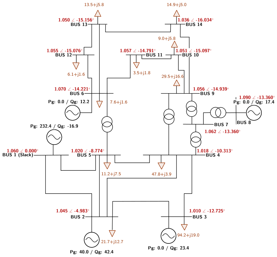
The IEEE 14-bus system (Figure 2) is a benchmark test network commonly employed in power flow and voltage stability studies. The system comprises 14 buses; five synchronous generators located at buses 1 (slack), 2, 3, 6, and 8; and a set of meshed transmission lines. The total load demand is approximately 259 MW and 73.5 Mvar, distributed across multiple load buses. The model includes tap-changing transformers and standard transmission system parameters. Given its moderate size and topological complexity, this system is appropriate for validating steady-state voltage profile assessment methodologies [31].

4.3. The IEEE 30-Bus System

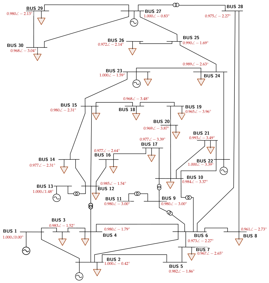
The IEEE 30-bus system, depicted in Figure 3, is a well-established benchmark for power flow studies and power system behavior analysis. This network comprises 30 buses, six generators, and multiple transmission lines arranged in a meshed topology. Bus 1 serves as the slack bus, while the remaining generators are located at buses 2, 5, 8, 11, and 13, supplying active and reactive power to the system.

The network features numerous load buses distributed throughout the system, with an approximate total demand of 283 MW and 126 Mvar. Tap-changing transformers are also included to regulate voltage levels across different zones of the system. Given its intermediate size and complexity, this test system is well suited for analyzing voltage profiles, power flow distributions, and steady-state operating conditions [31].

4.4. The IEEE 57-Bus System

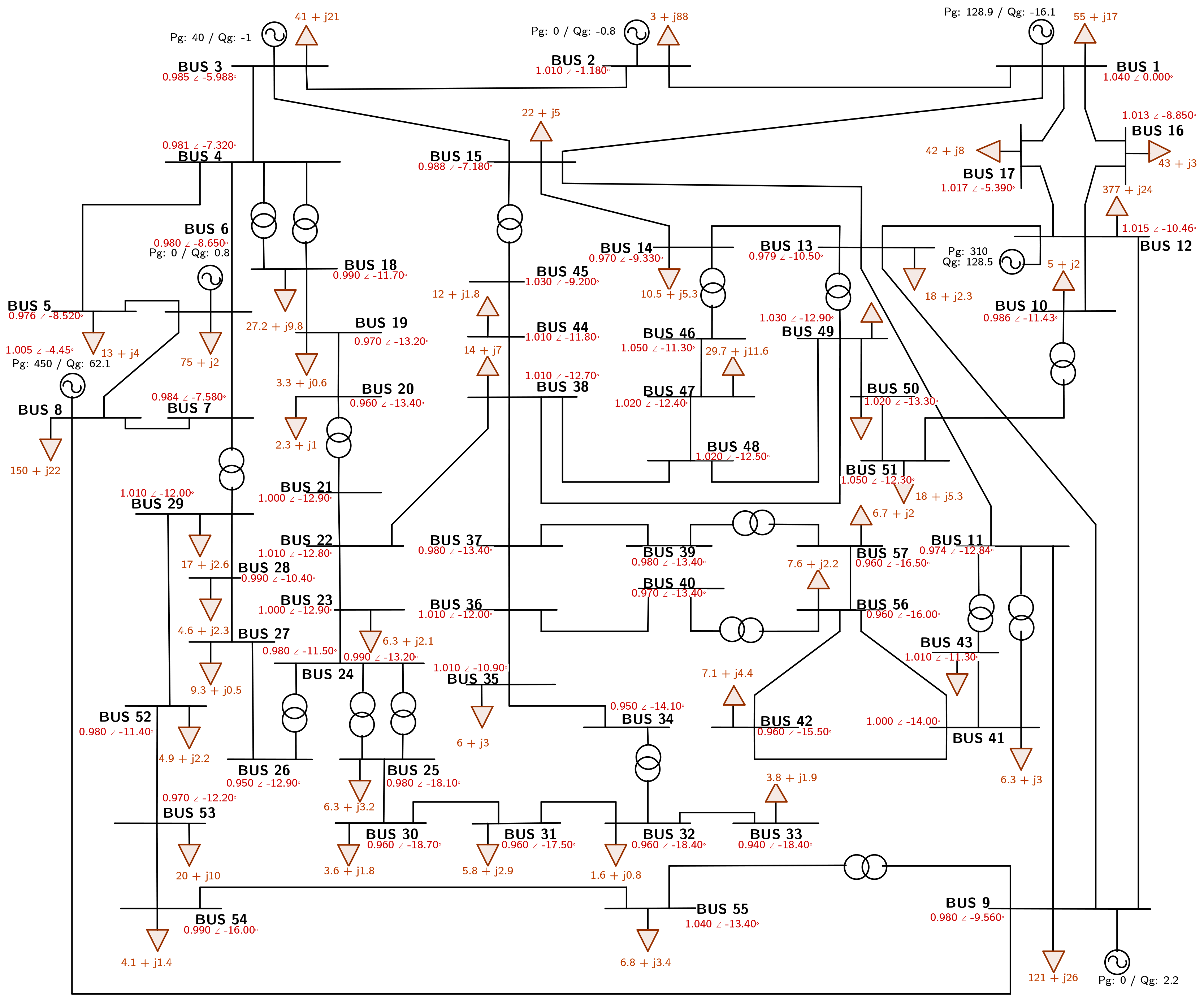
The IEEE 57-bus system, shown in Figure 4, is a larger-scale test network used for voltage stability studies and steady-state behavior analysis of power systems. It comprises 57 buses interconnected by transmission lines and transformers, along with seven generators that supply the power required to meet system demand. Bus 1 is designated as the slack bus, while the remaining generators provide active and reactive power support across different zones of the network.

The loads are distributed throughout the system, enabling the analysis of voltage profile variations in response to changes in demand. Tap-changing transformers are also included to facilitate the study of voltage regulation and its impact on stability margins. Due to its size and complexity, the IEEE 57-bus system is well suited for evaluating critical operating conditions and analyzing system behavior under voltage stability scenarios [31].

5. Numerical Validations and Results Analysis

The proposed framework was implemented in MATLAB (version R2025b) for the heuristic model, considering that the most critical contingency is the one that yields the lowest stability margin [33]. In contrast, the NLP method and the convex model were implemented in the Julia programming language (version 1.12.2), using Visual Studio Code as the development environment, enabling the exploitation of advanced optimization capabilities and a high computational performance. All simulations were carried out on a personal computer equipped with an AMD Ryzen processor (3.30 GHz), 16 GB of RAM, and a 64-bit version of Microsoft Windows 11 Pro. To ensure data consistency and minimize the potential errors associated with data handling, all system parameters were directly imported from the MATPOWER library during algorithm execution.

The following sections present the results obtained for the different case studies considered, including the NLP model, the heuristic approach, and the convex formulation. These results are analyzed for each transmission line contingency in the evaluated systems, enabling a comprehensive comparison of the performance of the proposed methodologies.

It should be highlighted that, in some larger systems, particularly the IEEE 30- and 57-bus feeders, certain contingencies led to the formation of electrical islands within the network. In such cases, the disconnection of specific transmission lines caused the system to split into two or more independent subsystems, each characterized by distinct operating conditions and stability margins. Consequently, the contingencies that resulted in islanding were excluded from the analysis, as the objective of this study is to evaluate system behavior under connected operating conditions and to ensure a consistent basis for comparing the proposed approaches.

Remark 5.

From a practical standpoint, islanding conditions introduce additional complexities that fall outside the scope of conventional voltage stability margin assessments. In particular, the resulting subsystems may lack a slack bus, exhibit infeasible power flow conditions, or require independent re-dispatch strategies, thereby invalidating the assumptions of the proposed models. As a result, excluding such contingencies ensures methodological consistency and avoids the misinterpretation of the stability margins across different solution approaches.

5.1. IEEE 9-Bus Case

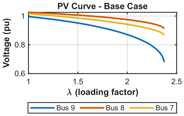
As seen in the $P-V$ curve, the system exhibits a maximum voltage stability margin of $2.37$, which corresponds to an increase of approximately $137\%$ relative to the nominal load under normal operating conditions. This result indicates that, in the base case, the system has a relatively high capacity to withstand demand increases before reaching the voltage collapse point.

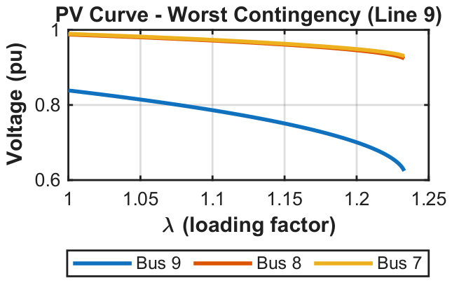
When evaluating transmission line contingencies, the most critical condition identified is the disconnection of line 4–9, where the stability margin decreases to $1.23$. This value implies that the system can only withstand an approximate $23\%$ increase in demand before reaching the critical operating point.

The voltage profile analysis (Figure 5) shows that, under this contingency, the voltage at bus 9 experiences a significant reduction, reaching a decrease of nearly $8.235\%$ with respect to the base case (Figure 6) and approximately $32.394\%$ relative to the other critical voltages in the contingency scenario. This behavior reveals that this bus constitutes one of the most sensitive points of the system regarding voltage instability phenomena.

From a topological perspective, the system features a meshed structure with low redundancy, characterized by the absence of parallel transmission lines. This condition limits the system’s ability to redistribute power flows after the loss of transmission elements. In particular, under the analyzed contingency, the power supply from the slack bus requires an increased flow through line 4–5, causing a progressive overload. Consequently, once the operating limits of this line are reached, the system tends to experience a voltage collapse, which is reflected in the proximity to the nose point of the $P-V$ curve.

To justify the fixed increment step $\Delta \lambda =0.001$ used in the heuristic method, a sensitivity analysis was carried out on the IEEE 9-bus system using three step sizes: $\Delta \lambda \in \{0.01,0.001,0.0001\}$. As shown in

Table 1. Sensitivity analysis of the load increment step $\Delta \lambda$ on the IEEE 9-bus system. Note: Ln denotes the contingency corresponding to the disconnection of line n. The Average error is computed relative to $\Delta \lambda =0.0001$ (reference).

$\mathbf{\Delta }\mathit{\lambda }$	${\mathit{\lambda }}_{max}$ (p.u.)						Time (s)	Avg. Error (%)
	L2	L3	L5	L6	L8	L9
0.0100	1.6400	2.1400	2.1000	1.9000	1.9300	1.2300	11.142	0.321
0.0010	1.6480	2.1440	2.1040	1.9060	1.9360	1.2330	11.919	0.033
0.0001	1.6484	2.1445	2.1045	1.9069	1.9363	1.2338	20.439	—

, the critical loading factors obtained with $\Delta \lambda =0.001$ differ from those obtained with the finest resolution ($\Delta \lambda =0.0001$) by an average relative error of only $0.033\%$, while the computation time increases from $11.9\mathrm{s}$ to $20.4\mathrm{s}$ when moving to the finer step. In contrast, $\Delta \lambda =0.01$ introduces an average error of $0.321\%$, with negligible time savings. Therefore, $\Delta \lambda =0.001$ provides an adequate balance between precision and computational efficiency and was adopted for all case studies. Regarding the Newton–Raphson power flow solver, the default MATPOWER implementation was used with a convergence tolerance of ${10}^{-8}$ p.u. on the power mismatch norm.

After implementing the heuristic and convex solution described in Section 3, the percentage error between the reference NLP solution and both approaches was calculated using the following expression:

$$\epsilon ={\displaystyle \frac{|{\lambda }_{\mathrm{NLP}}-{\lambda }_{\mathrm{method}}|}{{\lambda }_{\mathrm{NLP}}}}\times 100\%$$

(13)

The results presented in

Table 2. Maximum loadability (${\lambda }_{max}$) under line contingencies—IEEE 9-bus system. Note: The abbreviation p.u. refers to the per-unit system.

Line	From Bus	To Bus	${\mathit{\lambda }}_{max}$ (p.u.)			Error (%)
			NLP	Heuristic	Convex	Heur.	Conv.
2	4	5	1.648	1.647	1.648	0.061	0
3	5	6	2.145	2.143	2.145	0.093	0
5	6	7	2.105	2.103	2.105	0.095	0
6	7	8	1.907	1.905	1.907	0.105	0
8	8	9	1.936	1.935	1.936	0.052	0
9	9	4	1.234	1.232	1.234	0.162	0

demonstrate that both the heuristic method and the convex formulation estimate the voltage stability margin with high accuracy for the all contingencies analyzed in the IEEE 9-bus system. The percentage error of the heuristic approach ranges from $0.052\%$ (line 8–9) to $0.162\%$ (line 9–4), with an average of $0.095\%$ over the six evaluated contingencies, whereas the convex formulation exactly reproduces the reference value in all cases, yielding zero error.

Furthermore, the critical contingency corresponding to the disconnection of line 9–4, which produces the lowest stability margin (${\lambda }_{max}=1.234 \mathrm{p}.\mathrm{u}.$), is correctly identified by both methods: with an error of only 0.162% for the heuristic approach and with zero error for the convex formulation. This demonstrates not only the accuracy of the approximations but also their ability to consistently identify the most severe scenario.

5.2. IEEE 14-Bus Case

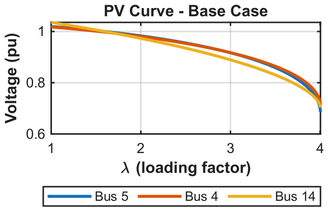
In the IEEE 14-bus system, the base case exhibits a higher load-carrying capacity, allowing for an increase of up to $\lambda =4.004$, representing approximately four times the nominal demand. This value exceeds that of the IEEE 9-bus system by approximately $68.7\%$, evidencing a greater structural robustness in the topology of the 14-bus system. This characteristic is largely due to the fact that several generators have redundant transmission paths, providing more than one route to deliver power to different points in the network.

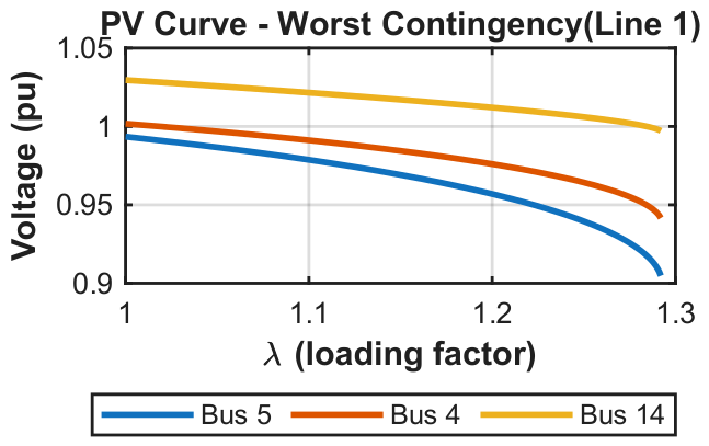
The most critical contingency occurs when the line connecting buses 1 and 2 is disconnected, both of which are generation-associated nodes. Under this condition, the voltage stability margin decreases to a value of $1.292$. In contrast to the behavior observed in the IEEE 9-bus system, where the contingency causes a voltage drop at nodes adjacent to the disconnected line, the opposite behavior occurs in this case. As shown in Figure 7, the critical nodes exhibit voltages slightly higher than those of the base case (Figure 8), even though the stability margin decreases dramatically. This behavior is explained by the fact that line 1–2 absorbs a significant amount of reactive power. Upon its disconnection, this absorption ceases, and the reactive power is redistributed towards nearby nodes through lower-impedance paths, thereby increasing the voltage. However, the loss of this main transmission route severely limits the system’s ability to withstand load increases, leading to an early voltage collapse.

As with the IEEE 9-bus system, both voltage stability margin estimation methods were applied to all contingencies of the IEEE 14-bus system. The results are presented in

Table 3. Maximum loadability (${\lambda }_{max}$) under line contingencies—IEEE 14-bus system. Note: The abbreviation p.u. refers to the per-unit system.

Line	From Bus	To Bus	${\mathit{\lambda }}_{max}$ (p.u.)			Error (%)
			NLP	Heuristic	Convex	Heur.	Conv.
1	1	2	1.288	1.291	1.290	0.233	0.155
2	1	5	3.645	3.664	3.710	0.521	1.783
3	2	3	2.258	2.268	2.274	0.443	0.709
4	2	4	3.255	3.270	3.508	0.461	7.773
5	2	5	3.390	3.410	3.686	0.590	8.732
6	3	4	3.893	3.923	4.057	0.771	4.213
7	4	5	3.912	3.928	4.061	0.409	3.809
11	6	11	3.508	3.566	3.673	1.653	4.704
12	6	12	3.927	3.952	4.233	0.637	7.792
13	6	13	3.214	3.265	3.297	1.587	2.582
16	9	10	3.951	3.977	4.272	0.658	8.125
17	9	14	3.702	3.700	3.714	0.054	0.324
18	10	11	3.708	3.757	3.914	1.321	5.556
19	12	13	3.970	3.995	4.290	0.630	8.060
20	13	14	3.231	3.311	3.341	2.476	3.405

. Unlike the previous case, the convex method exhibits nonzero errors for most contingencies, with a maximum error of $8.732\%$ and an average error of $4.515\%$. The heuristic method, in contrast, demonstrates a superior performance, with a maximum error of $2.476\%$ and an average error of $0.830\%$. Despite this difference in accuracy, both methods successfully identify the worst system contingency, i.e., the disconnection of line 1 (1–2), with a low margin of error.

5.3. IEEE 30-Bus Case

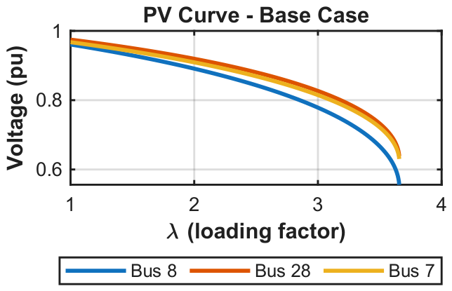
The IEEE 30-bus system reaches a maximum stability margin of ${\lambda }_{max}=3.648$, equivalent to a $264\%$ overload relative to the nominal demand, positioning it as the second most robust system among the analyzed cases. This capacity can be attributed to its topology and the fact that most generators have at least four transmission routes, which efficiently distributes the power flows when faces with load increases.

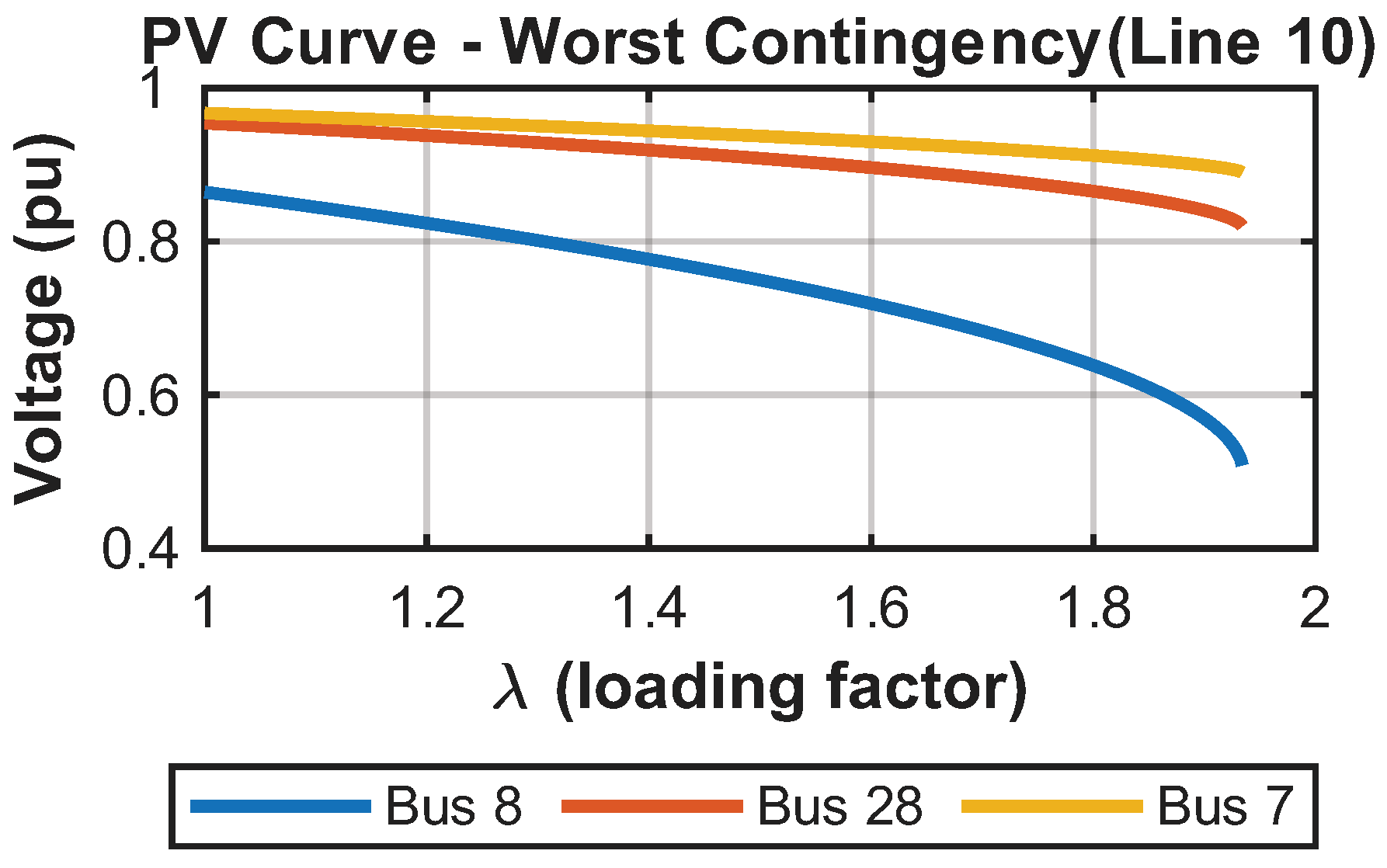
Regarding contingencies, the most critical corresponds to the disconnection of line 6–8, which reduces the margin to $\lambda =1.934$. Upon the loss of this route, line 28–8 absorbs the redistributed flow, increasing the current and causing a voltage drop of $9.29\%$ at bus 8 with respect to the base case, as illustrated in Figure 9 and Figure 10.

At the opposite extreme, the outage of lines 22–24 and 23–24 is practically harmless to the system, with ${\lambda }_{max}=3.656$, a value nearly identical to that of the base case. Both lines share bus 24, which operates as an intermediate load node without significant participation in the main power transfer routes.

Unlike the IEEE 14-bus system, the 30-bus feeder exhibits smaller errors for both the heuristic and convex methods, with the maximum error of the former decreasing from $8.732\%$ to $2.307\%$. This behavior is primarily attributed to the more meshed topology of the 30-bus system: by having a greater number of alternative transmission routes, the redistribution of power flows under a contingency is more uniform, which is why the relaxed problem solution more closely approximates the reference NLP solution. In the 14-bus system, the lower network redundancy causes the flows to concentrate on a few routes when a line is disconnected, increasing the nonlinearities of the nodal balance equations and reducing the accuracy of the convex relaxation. This improved approximation can be clearly observed in

Table 4. Maximum loadability (${\lambda }_{max}$) under line contingencies–IEEE 30-bus system. Note: The row in bold corresponds to the worst contingency. Line 34 (25–26) creates an electrical island upon disconnection.

Line	From Bus	To Bus	${\mathit{\lambda }}_{max}$ (p.u.)			Error (%)
			NLP	Heuristic	Convex	Heur.	Conv.
1	1	2	2.111	2.110	2.113	0.047	0.095
2	1	3	3.258	3.256	3.259	0.061	0.031
3	2	4	3.139	3.137	3.148	0.064	0.287
4	3	4	3.291	3.289	3.292	0.061	0.030
5	2	5	3.214	3.212	3.229	0.062	0.467
6	2	6	2.978	2.976	2.988	0.067	0.336
7	4	6	3.208	3.207	3.282	0.031	2.307
8	5	7	3.213	3.211	3.228	0.062	0.467
9	6	7	3.530	3.530	3.530	0.000	0.000
10	6	8	1.935	1.933	1.958	0.103	1.189
17	12	14	3.626	3.624	3.649	0.055	0.634
18	12	15	3.552	3.550	3.575	0.056	0.648
19	12	16	3.619	3.618	3.643	0.028	0.663
20	14	15	3.656	3.655	3.681	0.027	0.684
21	16	17	3.647	3.646	3.671	0.027	0.658
22	15	18	3.598	3.596	3.621	0.056	0.639
23	18	19	3.641	3.640	3.666	0.027	0.687
24	19	20	3.586	3.585	3.610	0.028	0.669
25	10	20	3.357	3.355	3.394	0.060	1.102
26	10	17	3.489	3.488	3.513	0.029	0.688
27	10	21	3.477	3.476	3.498	0.029	0.604
28	10	22	3.571	3.570	3.593	0.028	0.616
29	21	22	3.351	3.350	3.369	0.030	0.537
30	15	23	3.602	3.600	3.624	0.056	0.611
31	22	24	3.653	3.651	3.678	0.055	0.684
32	23	24	3.653	3.651	3.677	0.055	0.657
33	24	25	3.643	3.642	3.667	0.027	0.659
34	25	26	Electrical island
35	25	27	3.601	3.600	3.624	0.028	0.639
37	27	29	3.248	3.247	3.248	0.031	0.000
38	27	30	2.705	2.703	2.705	0.074	0.000
39	29	30	3.637	3.635	3.661	0.055	0.660
40	8	28	3.626	3.625	3.650	0.028	0.662
41	6	28	3.542	3.540	3.568	0.056	0.734

, where most contingencies exhibit error values below 3% for the convex formulation and below 0.1% for the heuristic method, demonstrating the higher consistency of both approaches in more interconnected networks.

5.4. IEEE 57-Bus Case

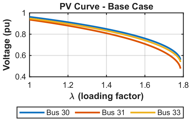
The IEEE 57-bus system yields a voltage stability margin of $1.785$ in the base case, which makes it the system with the lowest margin among the analyzed cases. Its larger number of buses and elements than smaller networks does not imply greater robustness against load increases, since the topology features zones with low connection redundancy that limit power flow redistribution under disturbances.

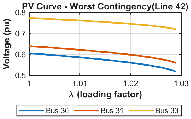
As identified in the contingency analysis, the most critical condition corresponds to the disconnection of line 42, which connects buses 25 and 30, with a stability margin of merely $1.022$, representing a $2.2\%$ increase above the nominal load (Figure 11). This situation is critical due to the combination of three unfavorable factors: the absence of local generation in the area, an almost radial topology, and the fact that, following the disconnection, bus 30 is left with only one alternative high-impedance route.

As evidenced by the voltage profiles shown in Figure 11 and Figure 12, bus 30 experiences the most severe voltage degradation with respect to the base case, exhibiting a pronounced voltage drop under the contingency scenario. This behavior confirms the high sensitivity of this area to transmission line outages and highlights its reduced capability to sustain additional load increases before reaching voltage collapse conditions.

Another critical case is line 47, between buses 34 and 35, which constitutes a particular case since the reference NLP method (IPOPT) failed to converge for this contingency, even when multiple starting points were used. This can be attributed to the resulting topology, which generates a feasible space with high nonlinearity where the solver becomes trapped in regions of numerical infeasibility. The heuristic method and the convex formulation report ${\lambda }_{max}=1.068$ p.u. and ${\lambda }_{max}=1.010$ p.u., respectively, values that are consistent with each other, suggesting that the system can operate under this contingency, although it was not possible to verify this with the reference method, as observed in

Table 5. Maximum loadability (${\lambda }_{max}$) under line contingencies—IEEE 57-bus system. Note: The row in bold corresponds to the worst contingency. Lines 45 (32–33) and 48 (35–36) create an electrical island upon disconnection and line 47 (34–35) did not converge with the NLP method.

Line	From Bus	To Bus	${\mathit{\lambda }}_{max}$ (p.u.)			Error (%)
			NLP	Heuristic	Convex	Heur.	Conv.
1	1	2	1.660	1.675	1.681	0.904	1.265
2	2	3	1.663	1.678	1.685	0.902	1.323
3	3	4	1.612	1.634	1.700	1.365	5.459
4	4	5	1.738	1.771	1.844	1.899	6.099
5	4	6	1.727	1.759	1.822	1.853	5.501
6	6	7	1.736	1.769	1.846	1.901	6.336
7	6	8	1.751	1.785	1.848	1.942	5.540
8	8	9	1.719	1.752	1.791	1.920	4.188
9	9	10	1.746	1.781	1.854	2.005	6.186
10	9	11	1.721	1.753	1.823	1.859	5.927
11	9	12	1.749	1.783	1.858	1.944	6.232
12	9	13	1.736	1.769	1.848	1.901	6.452
13	13	14	1.716	1.748	1.839	1.865	7.168
14	13	15	1.720	1.752	1.847	1.860	7.384
15	1	15	1.676	1.678	1.727	0.119	3.043
16	1	16	1.665	1.688	1.771	1.381	6.366
17	1	17	1.651	1.672	1.754	1.272	6.239
18	3	15	1.690	1.720	1.822	1.775	7.811
21	5	6	1.742	1.775	1.847	1.894	6.028
22	7	8	1.710	1.745	1.814	2.047	6.082
23	10	12	1.732	1.765	1.841	1.905	6.293
24	11	13	1.740	1.774	1.857	1.954	6.724
25	12	13	1.680	1.712	1.789	1.905	6.488
26	12	16	1.695	1.722	1.803	1.593	6.372
27	12	17	1.683	1.709	1.789	1.545	6.298
28	14	15	1.712	1.745	1.824	1.928	6.542
29	18	19	1.729	1.760	1.842	1.793	6.536
30	19	20	1.741	1.773	1.857	1.838	6.663
32	21	22	1.750	1.782	1.867	1.829	6.686
33	22	23	1.534	1.579	1.580	2.934	2.999
34	23	24	1.641	1.689	1.702	2.925	3.717
38	26	27	1.577	1.613	1.658	2.283	5.136
39	27	28	1.482	1.514	1.541	2.159	3.981
40	28	29	1.383	1.411	1.425	2.025	3.037
42	25	30	1.022	1.029	1.043	0.685	2.055
43	30	31	1.361	1.370	1.407	0.661	3.380
44	31	32	1.523	1.592	1.571	4.531	3.152
45	32	33	Electrical island
47	34	35	−	1.068	1.010	—	—
48	35	36	Electrical island
49	36	37	1.256	1.297	1.292	3.264	2.866
50	37	38	1.175	1.207	1.193	2.723	1.532
51	37	39	1.753	1.787	1.862	1.940	6.218
52	36	40	1.760	1.794	1.866	1.932	6.023
53	22	38	1.603	1.652	1.652	3.057	3.057
55	41	42	1.695	1.725	1.780	1.770	5.015
57	38	44	1.703	1.739	1.784	2.114	4.756
60	46	47	1.614	1.648	1.689	2.107	4.647
61	47	48	1.702	1.738	1.794	2.115	5.405
62	48	49	1.740	1.775	1.845	2.011	6.034
63	49	50	1.745	1.779	1.862	1.948	6.705
64	50	51	1.702	1.736	1.811	1.998	6.404
67	29	52	1.445	1.487	1.445	2.907	0.000
68	52	53	1.755	1.788	1.772	1.880	0.969
69	53	54	1.731	1.767	1.834	2.080	5.950
70	54	55	1.719	1.754	1.818	2.036	5.759
72	44	45	1.669	1.704	1.745	2.097	4.554
74	56	41	1.730	1.764	1.828	1.965	5.665
75	56	42	1.746	1.781	1.845	2.005	5.670
77	57	56	1.736	1.770	1.845	1.959	6.279
78	38	49	1.722	1.757	1.823	2.033	5.865
79	38	48	1.665	1.702	1.756	2.222	5.465

.

In terms of accuracy, the heuristic method exhibits the lowest error with respect to the reference method throughout the entire table. However, its computation time for the 57-bus system was $16.6$ min, compared to $0.31$ min using the convex method. This reveals a trade-off between accuracy and computational efficiency: the heuristic method is more accurate but significantly more time-consuming, while the convex method offers a fast solution with errors that do not exceed $7\%$ in most cases, making it a practical alternative for larger-scale systems or online analysis.

5.5. Comparative Analysis of the Results

Table 6. Comparative summary of results across IEEE test systems.

Method	Test System	Worst Contingency	$\mathit{\lambda }$ Worst	Avg. Error (%)	Max. Error (%)	Time (min)
NPL	IEEE 9-bus	Line 9–4	1.234	-	-	0.02
	IEEE 14-bus	Line 1–2	1.288	-	-	0.03
	IEEE 30-bus	Line 6–8	1.935	-	-	0.08
	IEEE 57-bus	Line 25–30	1.022	-	-	0.41
Heuristic	IEEE 9-bus	Line 9–4	1.234	0.095	0.162	1.82
	IEEE 14-bus	Line 1–2	1.291	0.830	2.476	14.10
	IEEE 30-bus	Line 6–8	1.933	0.046	0.103	31.33
	IEEE 57-bus	Line 25–30	1.029	1.954	4.531	16.60
Convex	IEEE 9-bus	Line 9–4	1.234	0	0	0.02
	IEEE 14-bus	Line 1–2	1.290	4.515	8.732	0.03
	IEEE 30-bus	Line 6–8	1.958	0.586	2.307	0.07
	IEEE 57-bus	Line 25–30	1.043	5.111	7.811	0.31

provides a compact comparative overview of the three methods (NPL, heuristic, convex) across the four IEEE test systems. For each method and system, the table reports the worst contingency (line outage), its corresponding critical loading factor $\lambda$, the average and maximum percentage errors with respect to the reference solution, and the total computation time. Islanding contingencies (where the network becomes disconnected) were excluded from all evaluations. Specifically, line 25–26 in the 30-bus system and lines 32–33, 35–36, and 34–35 in the 57-bus system were excluded. Among these, line 34–35 in the 57-bus system is noteworthy: the NPL method did not find a solution, whereas the heuristic and convex methods did. Nevertheless, it was excluded for consistency.

6. Conclusions

This paper presented a comparative analysis of three methodologies for estimating the voltage stability margin under transmission line contingencies: a reference NLP approach (IPOPT) with multi-start initialization, a recursive heuristic method based on successive Newton–Raphson power flow solutions, and a convex formulation using second-order cone programming. The evaluation was conducted on the IEEE 9-, 14-, 30-, and 57-bus test systems.

The convex formulation achieved zero error for all contingencies in the 9-bus system but exhibited nonzero errors as system size increased, reaching a maximum of $8.732\%$ in the 14-bus system and $2.307\%$ in the 30-bus system. This behavior can be attributed to network redundancy: more meshed topologies enable a uniform power flow redistribution, reducing nonlinearities and improving convex relaxation accuracy. Conversely, lower redundancy causes flow concentration on critical routes, increasing the approximation error.

The heuristic method demonstrated superior accuracy across all test systems, with maximum errors of $0.162\%$ (9-bus), $2.476\%$ (14-bus), $0.103\%$ (30-bus), and $4.531\%$ (57-bus). However, this accuracy came at a significant computational cost: for the 57-bus system, the heuristic required $16.6$ min vs. $0.31$ min for the convex formulation—a $54\times$ speedup. The convex method, with errors typically below $7\%$, represents a practical alternative for online contingency assessment, while the heuristic is better suited for offline planning studies.

For the 57-bus system, the reference method failed to converge for line 47 (34–35) due to a highly nonlinear feasible space, whereas both the heuristic and convex methods provided consistent estimates ($1.068$ p.u. and $1.010$ p.u., respectively), demonstrating their robustness. The study also confirmed that a larger number of buses does not ensure greater voltage stability; the 57-bus system exhibited the lowest base-case margin ($1.785$) due to the low redundancy and a near-radial topology in certain areas. The most critical contingencies were identified as line 9–4 (9-bus), line 1–2 (14-bus), line 6–8 (30-bus), and line 25–30 (57-bus), with the latter allowing only a $2.2\%$ load increase before collapse.

Several research directions emerge from this study. First, the methodologies could be extended to incorporate dynamic voltage stability analysis, including tap-changing transformers and protection system responses. Second, the integration of renewable energy sources with inherent intermittency and reduced inertia could be studied, which would require reformulating the loadability model to account for stochastic generation patterns. Third, tighter convex relaxations, such as higher-order cone programming or moment-based semidefinite programming hierarchies, could reduce approximation errors in low-redundancy networks. Fourth, the heuristic method’s computational efficiency could be improved through adaptive step-size control or parallelization for larger systems. Fifth, the islanding contingencies excluded from this analysis warrant dedicated study due to challenges related to slack bus absence and independent re-dispatch strategies. Finally, hybrid methods combining the accuracy of heuristic approaches with the speed of convex relaxations (using convex solutions as warm-start points for nonlinear optimization) could enable real-time voltage stability monitoring for large-scale power systems.

References

- Adebayo, I.; Sun, Y. New Performance Indices for Voltage Stability Analysis in a Power System. Energies 2017, 10, 2042. [Google Scholar] [CrossRef]
- Zhang, H.; Ou, Y.; Ren, M.; Sun, Y.; Wang, P. Progress on the Sustainable Development Goals in Asia requires ambitious climate targets combined with sustainability-focused measures. Commun. Earth Environ. 2026, 7, 126. [Google Scholar] [CrossRef]
- Zahid, H.; Zulfiqar, A.; Adnan, M.; Iqbal, M.S.; Shah, A.; Mohamed, S.E.G. Global renewable energy transition: A multidisciplinary analysis of emerging computing technologies, socio-economic impacts, and policy imperatives. Results Eng. 2025, 26, 105258. [Google Scholar] [CrossRef]
- ur Rehman, A.; Sanjari, M.J.; Elavarasan, R.M.; Jamal, T. Sustainability-aligned pathways for energy transition: A review of low-carbon energy network solutions. Renew. Sustain. Energy Rev. 2026, 226, 116428. [Google Scholar] [CrossRef]
- Milano, F.; Dörfler, F.; Hug, G.; Hill, D.J.; Verbič, G. Foundations and Challenges of Low-Inertia Systems (Invited Paper). In Power Systems Computation Conference (PSCC 2018); IEEE: Piscataway, NJ, USA, 2018; pp. 1–25. [Google Scholar] [CrossRef]
- Dobson, I.; Glavitsch, H.; Liu, C.C.; Tamura, Y.; Vu, K. Voltage collapse in power systems. IEEE Circuits Devices Mag. 1992, 8, 40–45. [Google Scholar] [CrossRef]
- Naik, S.; Khedkar, M.; Bhat, S. Effect of line contingency on static voltage stability and maximum loadability in large multi bus power system. Int. J. Electr. Power Energy Syst. 2015, 67, 448–452. [Google Scholar] [CrossRef]
- Salgado Duarte, Y.; del Castillo Serpa, A.M. Método heurístico para la evaluación de la confiabilidad en un subsistema de líneas de transmisión. Rev. Ing. Energética 2016, 37, 3–14. [Google Scholar]
- Bonini Neto, A.; Amancio Alves, D. Singularities Analysis of the Jacobian Matrix Modified in the Continuation Power Flow: Mathematical Modeling. IEEE Lat. Am. Trans. 2016, 14, 4750–4756. [Google Scholar] [CrossRef]
- Rinaudo, F.D.; Aromataris, L.M. Impacto de la generación eólica en estabilidad transitoria de sistemas eléctricos de potencia. In 2014 IEEE Biennial Congress of Argentina (ARGENCON); IEEE: Piscataway, NJ, USA, 2014; pp. 438–442. [Google Scholar] [CrossRef]
- Candelo, J.E.; Caicedo, G.; Castro, F. Methods for Voltage Stability Assessment in Power Systems. Inf. Tecnol. 2008, 19, 97–110. (In Spanish) [Google Scholar] [CrossRef]
- Tamayo-Guzmán, F.E.; Barrera-Singaña, C.A. Estabilidad en régimen permanente de sistemas eléctricos de potencia considerando límites de operación en generadores, transformadores y líneas de transmisión. Iteckne 2021, 18, 141–149. [Google Scholar] [CrossRef]
- Pedersen, A.S.; Blanke, M.; Johannsson, H. Convex relaxation of power dispatch for voltage stability improvement. In 2015 IEEE Conference on Control Applications (CCA); IEEE: Piscataway, NJ, USA, 2015; pp. 1528–1533. [Google Scholar] [CrossRef]
- Montoya, O.D.; Gil-González, W.; Arias-Londoño, A.; Rajagopalan, A.; Hernández, J.C. Voltage Stability Analysis in Medium-Voltage Distribution Networks Using a Second-Order Cone Approximation. Energies 2020, 13, 5717. [Google Scholar] [CrossRef]
- Wang, C.; Cui, B.; Wang, Z.; Gu, C. SDP-Based Optimal Power Flow with Steady-State Voltage Stability Constraints. IEEE Trans. Smart Grid 2019, 10, 4637–4647. [Google Scholar] [CrossRef]
- Ergun, H.; Dave, J.; Van Hertem, D.; Geth, F. Optimal Power Flow for AC-DC Grids: Formulation, Convex Relaxation, Linear Approximation, and Implementation. IEEE Trans. Power Syst. 2019, 34, 2980–2990. [Google Scholar] [CrossRef]
- Santos-Azevedo, M.S.; Pérez-Abril, I.; de León-Benítez, C.; Cabral-Leite, J.; Holanda-Bezerra, U. Multiobjective optimization of the reactive power compensation in electric distribution systems. Dyna 2014, 81, 175–183. [Google Scholar] [CrossRef]
- Bai, W.; Lee, K.Y.; Eke, I. Optimal Power Flow Considering Global Voltage Stability Based on a Hybrid Modern Heuristic Technique. IFAC-PapersOnLine 2022, 55, 413–418. [Google Scholar] [CrossRef]
- Kyomugisha, R.; Muriithi, C.M.; Edimu, M. Multiobjective optimal power flow for static voltage stability margin improvement. Heliyon 2021, 7, e08631. [Google Scholar] [CrossRef]
- Prabhakar, P.; Kumar, A. Voltage stability boundary and margin enhancement with FACTS and HVDC. Int. J. Electr. Power Energy Syst. 2016, 82, 429–438. [Google Scholar] [CrossRef]
- Coffrin, C.; Bent, R.; Sundar, K.; Ng, Y.; Lubin, M. PowerModels.jl: An Open-Source Framework for Exploring Power Flow Formulations. In Proceedings of the Power Systems Computation Conference 2018, Dublin, Ireland, 11–15 June 2018. [Google Scholar] [CrossRef]
- Wächter, A.; Biegler, L.T. On the implementation of an interior-point filter line-search algorithm for large-scale nonlinear programming. Math. Program. 2006, 106, 25–57. [Google Scholar] [CrossRef]
- Mokred, S.; Wang, Y. Voltage stability assessment and contingency ranking in power systems based on modern stability assessment index. Results Eng. 2024, 23, 102548. [Google Scholar] [CrossRef]
- Athay, T. An Overview of Power Flow Analysis. In Proceedings of the 1983 American Control Conference; IEEE: Piscataway, NJ, USA, 1983; pp. 404–410. [Google Scholar] [CrossRef]
- Niu, M.; Wan, C.; Xu, Z. A review on applications of heuristic optimization algorithms for optimal power flow in modern power systems. J. Mod. Power Syst. Clean Energy 2014, 2, 289–297. [Google Scholar] [CrossRef]
- Srivastava, L.; Dixit, S.; Agnihotri, G. Optimal Location and Size of TCSC for Voltage Stability Enhancement Using PSO-TVAC. In 2014 Power and Energy Systems Conference: Towards Sustainable Energy (PESTSE); IEEE: Piscataway, NJ, USA, 2014. [Google Scholar] [CrossRef]
- Kulworawanichpong, T. Simplified Newton–Raphson power-flow solution method. Int. J. Electr. Power Energy Syst. 2010, 32, 551–558. [Google Scholar] [CrossRef]
- Mokred, S.; Wang, Y.; Chen, T. A Novel Collapse Prediction Index for Voltage Stability Analysis and Contingency Ranking in Power Systems. Prot. Control Mod. Power Syst. 2023, 8, 1–27. [Google Scholar] [CrossRef]
- Zhang, F.; Shen, Z.; Xu, W.; Wang, G.; Yi, B. Optimal Power Flow Algorithm Based on Second-Order Cone Relaxation Method for Electricity-Gas Integrated Energy Microgrid. Complexity 2021, 2021, 2073332. [Google Scholar] [CrossRef]
- Garces, A. Mathematical Programming for Power Systems Operation with Applications in Python: From Theory to Applications in Python; Wiley: Hoboken, NJ, USA, 2021. [Google Scholar] [CrossRef]
- Zimmerman, R.D.; Murillo-Sánchez, C.E.; Thomas, R.J. MATPOWER: Steady-State Operations, Planning, and Analysis Tools for Power Systems Research and Education. IEEE Trans. Power Syst. 2011, 26, 12–19. [Google Scholar] [CrossRef]
- Anderson, P.M.; Fouad, A.A.A. Power System Control and Stability, 2nd ed.; IEEE Press/Wiley-Interscience: Piscataway, NJ, USA, 2003. [Google Scholar]
- Liu, Q.; Song, Y.; Jiang, Y.; Xu, Y.; Chen, S. Coordinated voltage control for improved power system voltage stability. Front. Energy Res. 2023, 10, 1088563. [Google Scholar] [CrossRef]
Figure 1.
IEEE 9-bus test system—Base case: bus voltage magnitude profile.
Figure 2.
IEEE 14-bus test system—Base case: nodal voltage profile.
Figure 3.
IEEE 30-bus test system—Base case: nodal voltage profile.
Figure 4.
IEEE 57-bus test system—Base case: nodal voltage profile.
Figure 5.
Voltage profile for the most critical nodes in the IEEE 9-bus system.
Figure 6.
Voltage profile for the base case in the IEEE 9-bus system.
Figure 7.
Voltage profile for the most critical nodes in the IEEE 14-Bus system.
Figure 8.
Voltage profile for the base case in the IEEE 14-Bus system.
Figure 9.
Voltage profile for the base case IEEE 30-bus system.
Figure 10.
Voltage profile at the most critical nodes IEEE 30-bus system.
Figure 11.
Voltage profile in the most critical nodes in the IEEE 57-bus system.
Figure 12.
Voltage profile for the base case in the IEEE 57-bus system.