Lithium-Ion Battery SOH Prediction Method Based on Multidimensional Feature Data Fusion

Abstract

Aiming at the problem that the degradation mechanism of lithium-ion batteries is complex during aging and that a single feature is difficult to fully characterize the battery state of health (SOH), this paper proposes an SOH prediction method for lithium-ion batteries based on multidimensional HF weighted fusion. First, health features (HF) are extracted from the battery charge–discharge data, and the Pearson correlation coefficient is used to analyze the correlation between each HF and SOH. Based on this, a weighted fused feature matrix is constructed. Then, through the collaborative modeling of a convolutional neural network (CNN) and a bidirectional long short-term memory (BiLSTM), the joint extraction of local features and temporal features from multidimensional HF is realized. Meanwhile, manta ray foraging optimization (MRFO) is introduced to optimize key hyperparameters. Finally, experiments are conducted based on the CALCE dataset, and the prediction performance of the proposed method is evaluated through comparisons with different prediction models and an ablation experiment on HF fusion strategies. The results show that the proposed method achieves good prediction results on the CS2-35, CS2-36, and CS2-37 test batteries, with the lowest MAE of 1.134% and the highest R² of 0.963.

1. Introduction

In new energy vehicles, the battery management system (BMS) is responsible for monitoring battery operating conditions and supporting safe and efficient energy utilization. As one of the key indicators used to characterize battery status, the state of health (SOH) reflects the aging level and remaining service capability of a battery [1]. Owing to their high energy density, long cycle lifespan, low self-discharge characteristics, and relatively limited environmental burden, lithium-ion batteries have been widely applied in electric vehicles and energy storage systems. However, during repeated charge–discharge cycling, internal aging reactions gradually accumulate, leading to capacity loss and continuous SOH decline [2,3]. Therefore, accurate SOH estimation is essential for battery safety assessment, operation strategy optimization, and service-life management.

The SOH evolution of lithium-ion batteries is affected by electrochemical aging, operating conditions, and historical usage, showing nonlinear and strongly coupled characteristics. As a result, it is difficult to describe the actual battery health state using only one measurable parameter [4]. SOH estimation techniques can be broadly grouped into experimental testing methods [5], mechanism-based approaches, and data-driven approaches. In contrast to mechanism-based methods, data-driven approaches infer battery health directly from measured data, thereby avoiding the need to establish an accurate electrochemical model. Instead, they extract health features (HFs) from measurable operating data, such as voltage, current, temperature, and capacity, and establish the mapping relationship between HF and SOH through machine learning or deep learning models [6,7,8].

For example, Reference [9] adopted random forest for battery SOH estimation, and Reference [10] used extreme gradient boosting with an accuracy correction strategy to improve SOH prediction performance. Reference [11] introduced a feature selection strategy for identifying key variables from complex data. Reference [12] constructed HF from capacity degradation characteristics, entropy information, and correlation-related indicators, and then applied manifold learning to reduce feature dimensionality. Although such approaches can improve SOH estimation performance, their prediction accuracy remains strongly influenced by the representativeness of the input HFs. If the extracted HF fails to fully describe battery degradation or includes redundant information, the accuracy and generalization performance of the model may decline.

In addition to conventional charge–discharge data-based methods, fast electrochemical data, such as electrochemical impedance spectroscopy (EIS), have also been used for SOH estimation in recent years [13]. EIS-based methods can obtain electrochemical diagnostic information within a relatively short measurement time and are useful for rapid battery health assessment. However, their practical implementation usually requires additional impedance measurement equipment and specific test conditions [14]. In contrast, the method in this study extracts HFs from electrical signals during the charge–discharge process, including voltage, current, and time-related information, which can be obtained from conventional cycling data. It should be noted that the total time from measurement to analysis is difficult to compare quantitatively among different methods because it is affected by the type and amount of measured data, measurement protocol, feature extraction process, equipment conditions, and computing platform. Therefore, this study focuses on SOH prediction based on charge–discharge electrical signal features, while EIS-related fast electrochemical features will be further considered in future work.

With the development of deep learning, recurrent neural networks and their variants have been increasingly applied to battery state estimation and lifetime prediction. Reference [15] introduced a stacked BiLSTM network for remaining useful life prediction of supercapacitors, which provides useful insight into the modeling of degradation sequences. Reference [16] combined BiLSTM with a self-attention mechanism for SOH estimation, while Reference [17] optimized a BiLSTM model using the sparrow search algorithm. Reference [18] constructed a long short-term memory (LSTM)-based capacity prediction model to learn battery degradation trends from time-series data. References [19,20] combined filtering algorithms, temperature-related models, and deep learning methods to estimate SOH under different operating conditions. Reference [21] further investigated SOH estimation from a multi-time-scale perspective using Kalman filtering. These studies show that deep learning models can effectively capture temporal degradation patterns and have good potential in lithium-ion battery SOH prediction.

To improve the representation of complex aging information, multi-feature fusion, convolutional neural networks (CNNs), and attention mechanisms have been introduced in recent studies [22,23]. These methods enhance prediction performance by extracting local features, modeling temporal dependencies, and learning feature interactions. Although existing data-driven SOH estimation methods have achieved promising results, several limitations still remain. First, some studies only use a single type of HF or a limited number of degradation indicators, which may not be sufficient to characterize the complex aging behavior of lithium-ion batteries. Second, when multiple HFs are directly used as model inputs, the differences in their degradation relevance and contribution are often not fully considered. Redundant or weakly informative features may affect model training and reduce prediction stability. Third, the hyperparameters of deep learning models are commonly selected by experience, which may lead to unstable prediction performance and limit the reproducibility of the model.

To address these issues, this paper proposes an SOH prediction framework based on multidimensional HF weighted fusion and MRFO-CNN-BiLSTM. The main contributions of this study are summarized as follows. First, 11 HFs are extracted from charge–discharge duration, charging area, IC characteristics, voltage change rate, and time-ratio information so that battery aging can be described from multiple observable dimensions. Second, a Pearson correlation-based weighting strategy is introduced to adjust the contribution of different HFs while retaining all extracted features, thereby avoiding the direct removal of low-correlation but potentially complementary degradation information. Third, a CNN-BiLSTM model is constructed to learn local coupling relationships and bidirectional temporal degradation dependencies from the weighted fused HF matrix. Finally, MRFO is used to optimize key hyperparameters of the CNN-BiLSTM model, reducing the dependence on empirical parameter selection.

2. Multidimensional HF Selection and Weighted Fusion

In this study, four cells from the CALCE lithium-ion battery aging dataset [24], namely CS2-35, CS2-36, CS2-37, and CS2-38, are selected for feature construction and model verification. The main battery specifications and charge–discharge conditions are summarized in

Table 1. Experimental conditions and technical specifications of CALCE dataset.

Experimental Condition	Parameter	Technical Specification	Parameter
Rated capacity	1.1 Ah	Cathode material	Lithium cobalt oxide (LiCoO2)
Charging current	0.5 A	Charging mode	Constant current–constant voltage (CC–CV)
Charge cut-off voltage	4.2 V	Charge termination condition	Current drops below 0.05 A
Discharging current	1 A	Discharging mode	Constant current (CC)
Discharge cut-off voltage	2.7 V	Ambient temperature	25 ± 2 °C

. For each cycle, charging was performed in constant-current/constant-voltage mode, followed by constant-current discharging. These controlled cycling data provide voltage, current, capacity, and cycle information for subsequent HF extraction.

The SOH of each cell is calculated according to the ratio between the current available capacity and the rated capacity, as expressed in Equation (1):

$$\mathrm{SOH}={\displaystyle \frac{Q_C}{Q_R}}\times 100\%$$

(1)

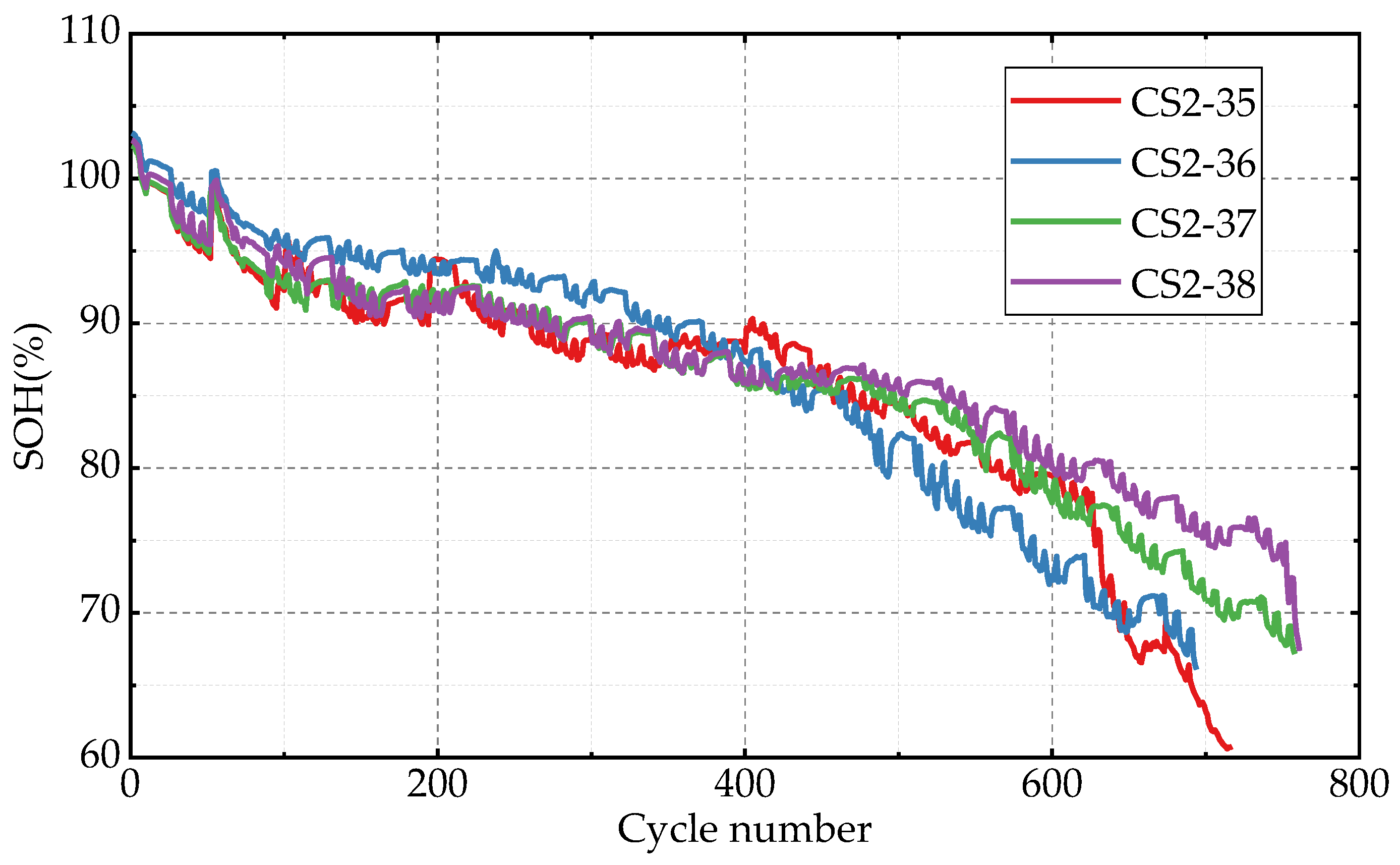
where Q_C and Q_R denote the current capacity and rated capacity of the battery, respectively. The SOH evolution curves of the four cells are shown in Figure 1. Overall, the SOH values decrease as the cycle number increases, while local fluctuations and different degradation rates can also be observed among different cells. These characteristics indicate that the battery aging process is not strictly monotonic, which increases the difficulty of SOH prediction under cross-cell conditions.

2.1. Multidimensional HF Selection

The construction of input HF directly determines how much degradation information can be provided to the prediction model. Instead of relying on a single external response, this paper describes battery aging from several observable changes in the charge–discharge process. Considering the variations in charge–discharge duration, current integration area, incremental capacity behavior, voltage variation rate, and time proportion during cycling, 11 HF indicators are extracted from multiple dimensions. These HF indicators correspond to different aging-related responses, including changes in charging time, discharge behavior, constant-voltage charging duration, incremental capacity (IC) curve evolution, and voltage dynamic characteristics. The detailed definitions of the extracted HF are listed in

Table 2. Health features of different dimensions extracted from charge–discharge curves.

No.	HF Description
HF1	Time difference for the voltage to rise from 3.8 V to 4.0 V during charging
HF2	Time difference for the voltage to decrease from 4.0 V to 3.8 V during discharging
HF3	Time from the beginning of charging to the voltage reaching 4.2 V
HF4	Time difference from the voltage reaching 4.2 V to the end of charging
HF5	Area under the current–time curve during the entire charging process
HF6	Area under the current–time curve from the beginning of charging to the voltage reaching 4.2 V
HF7	Area under the current–time curve from the voltage reaching 4.2 V to the end of charging
HF8	Peak value of the dQ/dV curve, namely the IC peak
HF9	Voltage corresponding to the IC peak
HF10	Minimum value of the voltage change rate dV/dt during charging
HF11	Ratio of the time from the beginning of charging to the voltage reaching 4.2 V to the total charging time

.

The selected HFs are related to battery aging from different physical perspectives. HF1–HF4 describe the time response of the battery during specific charging and discharging voltage intervals. As the battery ages, loss of active lithium, impedance growth, and polarization variation change the time required for the terminal voltage to pass through a given voltage range. HF5–HF7 are current–time integral features during different charging stages. Since the integral of current over time is directly related to the amount of charge transferred during charging, these area-related features can reflect the change in available capacity and charge acceptance ability during degradation. HF8 and HF9 are extracted from the IC curve. The IC peak and its corresponding voltage are sensitive to changes in electrochemical reaction processes, active material loss, and internal polarization, and therefore can characterize the evolution of battery aging from the perspective of voltage-capacity response. HF10 represents the minimum voltage change rate during charging, which reflects the dynamic voltage response and polarization behavior of the battery. HF11 describes the proportion of the charging time before reaching 4.2 V in the total charging time, reflecting the redistribution of charging duration between the constant-current and constant-voltage stages during aging. Therefore, the 11 HFs provide complementary information for SOH prediction from the perspectives of time response, charge accumulation, IC curve evolution, voltage dynamics, and charging-stage proportion.

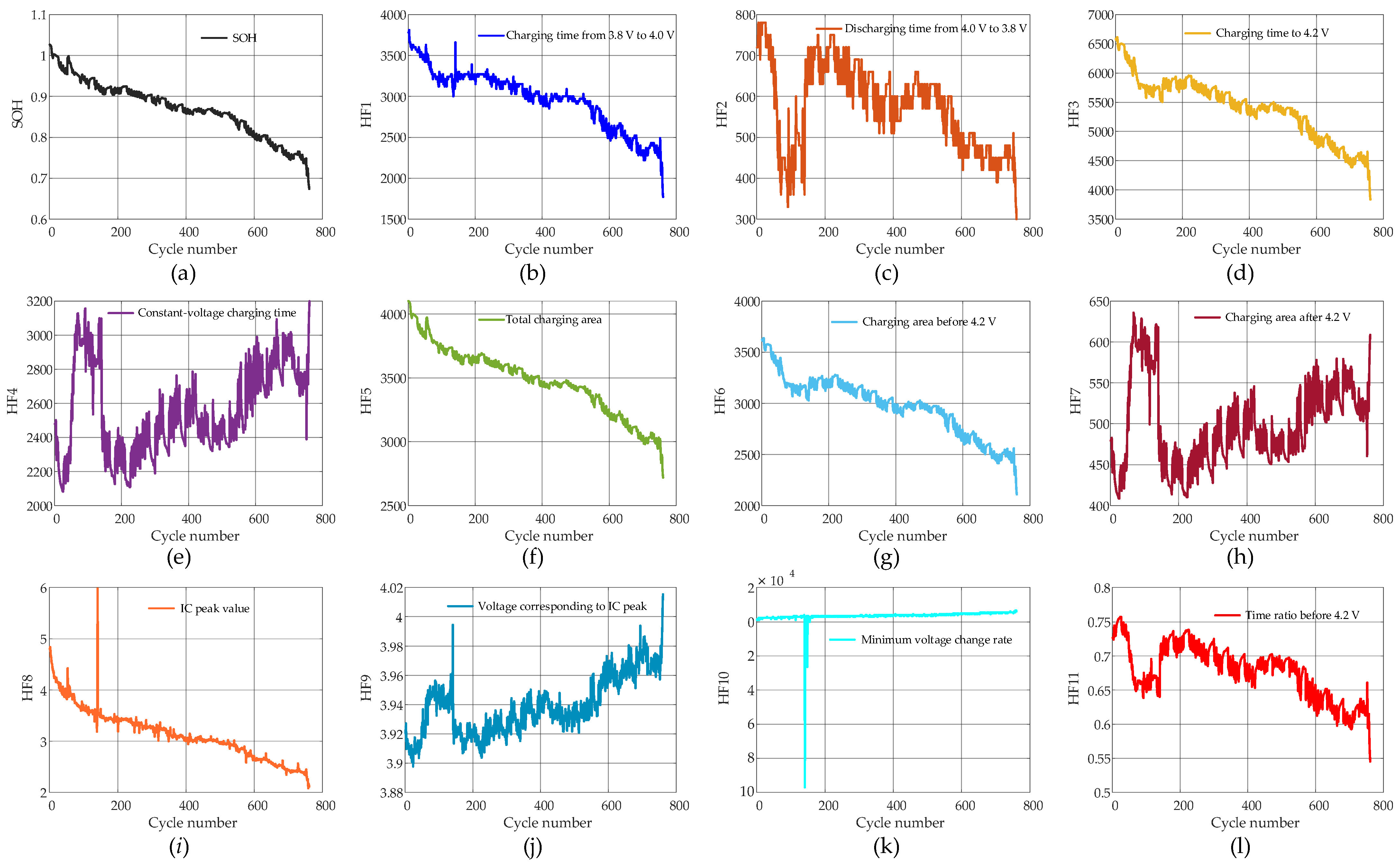
To illustrate the variation patterns of the extracted HF, the CS2-38 cell is taken as an example, and the evolution curves of SOH and 11 HF with cycle number are plotted in Figure 2. Different HFs show different changing trends during cycling, indicating that they describe battery degradation from different perspectives. Therefore, the extracted multidimensional HF can provide complementary information for subsequent SOH estimation.

To further describe the relationship between each HF and SOH, the Pearson correlation coefficient is used for quantitative analysis, as given in Equation (2):

$$r_i={\displaystyle \frac{{\displaystyle \sum _{k=1}^n}\left(x_{i,k}-{\overline{x}}_i\right)\left(y_k-\overline{y}\right)}{\sqrt{{\displaystyle \sum _{k=1}^n}{\left(x_{i,k}-{\overline{x}}_i\right)}^2}\sqrt{{\displaystyle \sum _{k=1}^n}{\left(y_k-\overline{y}\right)}^2}}}$$

(2)

where n denotes the number of samples; x_i,k represents the value of the i-th HF in the k-th sample; ${\overline{x}}_i$ is the average value of the i-th HF; y_k is the corresponding SOH value of the k-th sample; $\overline{y}$ is the average SOH value; and r_i denotes the Pearson correlation coefficient between the i-th HF and SOH.

2.2. Weighted Fusion of Multidimensional HF

The extracted HF has different physical meanings and numerical ranges. If they are directly used as model inputs, the training process may be affected by scale differences among features. Moreover, different HFs contribute unequally to SOH prediction. Some HFs are strongly correlated with SOH and reflect the main degradation trend, while others may provide local or auxiliary aging information. Therefore, this paper does not simply discard low-correlation HF. Instead, all 11 HFs are retained, and their contributions are adjusted through correlation-based weighting.

Before feature weighting, each HF is normalized to a unified numerical interval. This operation reduces the influence of feature magnitude differences and makes the subsequent weighting process more comparable. The normalized value of the i-th HF in the k-th sample is calculated by Equation (3).

$$x_{i,k}^{*}={\displaystyle \frac{x_{i,k}-x_{i,\min }}{x_{i,\max }-x_{i,\min }}}$$

(3)

where $x_{i,\min }$ and $x_{i,\max }$ denote the minimum and maximum values of the i-th HF among all samples, respectively.

After normalization, the correlation strength between each HF and SOH is used as the basis for assigning feature importance. Considering that both positive and negative correlations may reflect battery degradation characteristics, the magnitude of the Pearson correlation coefficient is used for weight assignment. In this way, features with stronger correlations are assigned larger weights, while weakly correlated features are retained with smaller contributions. The weight of the i-th HF is calculated as follows:

$$w_i={\displaystyle \frac{\left|r_i\right|}{{\displaystyle \sum _{j=1}^m}\left|r_j\right|}}$$

(4)

where m is the total number of HF indicators, and $m = 11$ in this paper; w_i is the weighting coefficient corresponding to the i-th HF, satisfying:

$${\displaystyle \sum _{i=1}^m}{w}_i=1$$

(5)

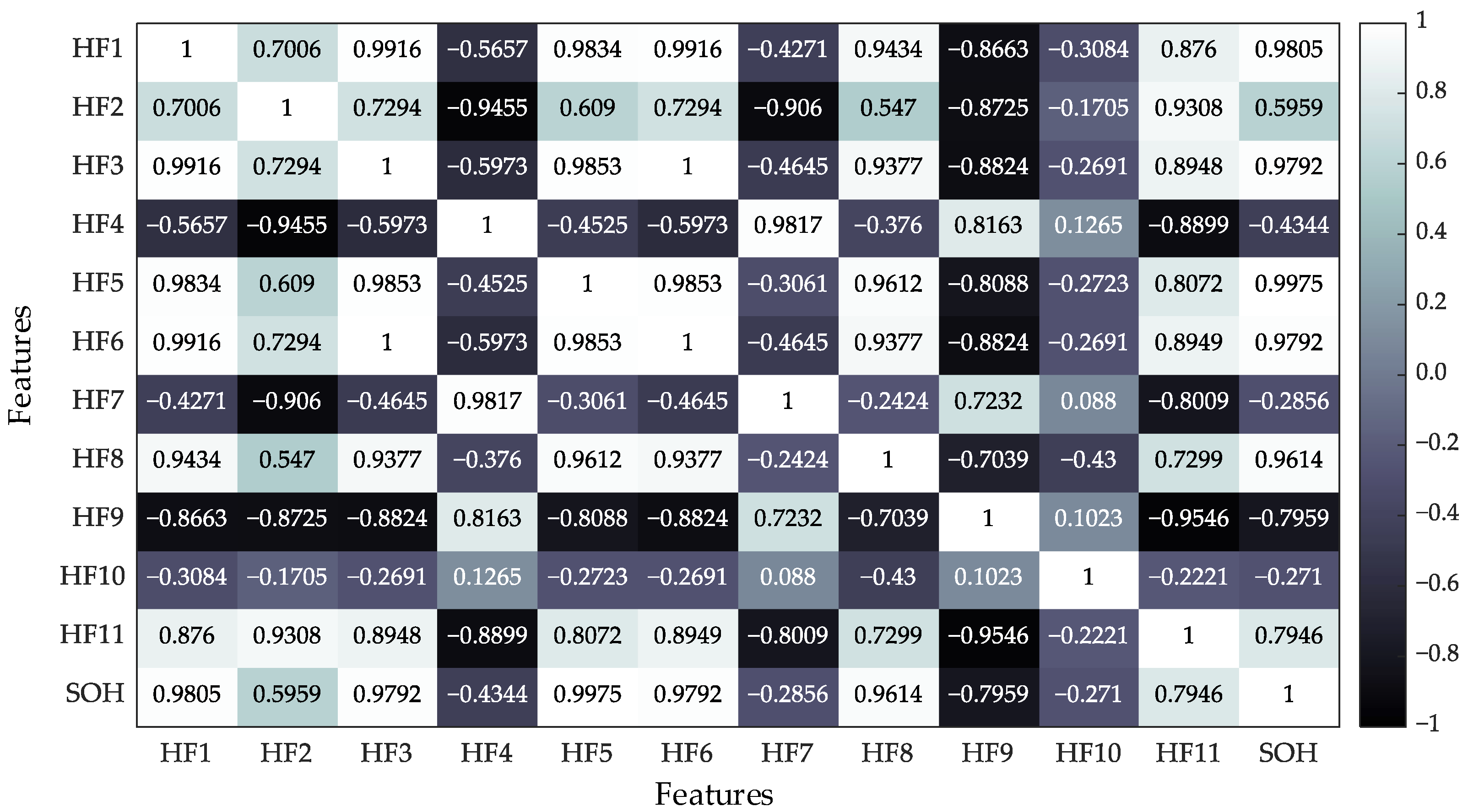
To show the correlation distribution more intuitively, the Pearson correlation coefficients among different HF and SOH are calculated and visualized in Figure 3. The heatmap shows that the correlations between different HF and SOH are not uniform. Some HF are highly correlated with SOH, while several HF show relatively weak correlations. Meanwhile, correlations also exist among different HFs, indicating that the extracted multidimensional HFs contain both redundant and complementary information. The weights of different HFs are determined according to their correlation strength with SOH, and the results are presented in

Table 3. Pearson correlation coefficients and weights of each HF.

Feature	ri	wi	Feature	ri	wi
HF1	0.9805	0.1214	HF7	−0.2856	0.0354
HF2	0.5959	0.0738	HF8	0.9614	0.1191
HF3	0.9792	0.1213	HF9	−0.7959	0.0986
HF4	−0.4344	0.0538	HF10	−0.2710	0.0336
HF5	0.9975	0.1235	HF11	0.7946	0.0984
HF6	0.9792	0.1213

.

Table 3 shows that the importance of different HF is not identical. HF5 obtains the largest weight, indicating that the current–time integral over the whole charging process has a close relationship with SOH. HF1, HF3, HF6, and HF8 also have relatively large weights, suggesting that charging time, staged charging area, and IC peak information are sensitive to battery aging. In contrast, HF4, HF7, and HF10 have smaller weights, but they still describe degradation-related changes from the constant-voltage charging stage, the later charging area, and the voltage response rate.

Therefore, the weight distribution does not mean that low-weight HF are useless. These HFs may not dominate the global degradation trend, but they can still provide supplementary information for local fluctuations or nonlinear aging behavior. For this reason, this paper retains all 11 HF and adjusts their contributions through weighting, rather than removing some features only according to their correlation values.

Although Pearson correlation mainly measures the linear relationship between each individual HF and SOH, it can provide a quantitative basis for evaluating the SOH-related degradation relevance of different HFs. In this study, the absolute Pearson correlation coefficient is used to adjust the relative input contribution of each HF before model training. HFs with stronger SOH-related degradation trends are assigned larger weights so that the subsequent CNN-BiLSTM model can focus more on the main degradation information during training. At the same time, low-correlation HFs are not directly removed because they may still contain supplementary information related to local fluctuations or aging differences among cells. Therefore, all 11 HFs are retained in the weighted fusion process. The weighted fused feature matrix provides more effective inputs for the subsequent CNN-BiLSTM model, thereby improving the model training effect and SOH prediction performance.

Furthermore, by combining the normalized HF indicators with their corresponding weights, a weighted fusion feature vector can be constructed. For the k-th sample, the weighted fused feature representation is expressed as

$${\mathbf{z}}_k=\left[w_1{x}_{1,k}^{*},w_2{x}_{2,k}^{*},\cdots ,w_m{x}_{m,k}^{*}\right]$$

(6)

Then, all samples can be represented as the weighted fused feature matrix:

$$\mathbf{Z}=\left[\begin{array}{cccc}{w}_1{x}_{1,1}^{*}& w_2{x}_{2,1}^{*}& \cdots & w_m{x}_{m,1}^{*}\\ w_1{x}_{1,2}^{*}& w_2{x}_{2,2}^{*}& \cdots & w_m{x}_{m,2}^{*}\\ ⋮& ⋮& \ddots & ⋮\\ w_1{x}_{1,n}^{*}& w_2{x}_{2,n}^{*}& \cdots & w_m{x}_{m,n}^{*}\end{array}\right]$$

(7)

where n is the number of samples; each row of matrix Z represents the weighted fused representation of one sample in the multidimensional HF space. After normalization and correlation-based weighting, the weighted fused feature matrix Z is obtained. This matrix comprehensively characterizes the differences in the contributions of different HF indicators to battery SOH and is used as the input of the subsequent CNN-LSTM prediction model to establish the mapping relationship between multidimensional HF and SOH.

3. SOH Prediction Model Based on MRFO-CNN-BiLSTM

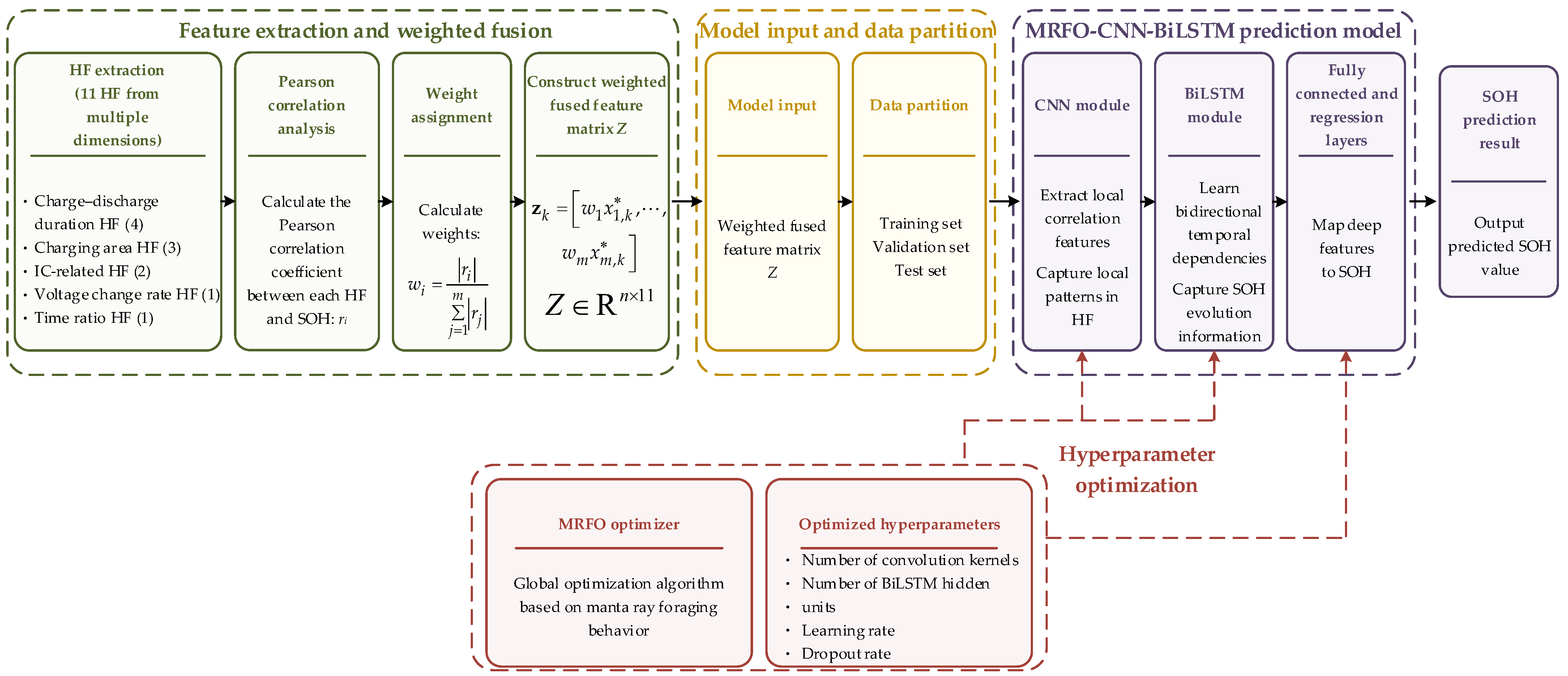
Based on the weighted fused feature matrix, an MRFO-CNN-BiLSTM model is developed for lithium-ion battery SOH prediction. In the proposed framework, the CNN part is responsible for extracting local coupling patterns from the fused HF sequence, while the BiLSTM part further learns the degradation dependencies along the cycling process. MRFO is used as an outer-loop optimizer to search for suitable hyperparameters of the CNN-BiLSTM model. The overall framework is shown in Figure 4.

3.1. CNN-BiLSTM Network Structure

The CNN-BiLSTM network used in this paper is designed to process the weighted fused HF sequence. The input layer receives the fused feature matrix $Z$, and the front part of the network contains two one-dimensional convolutional layers. These convolutional layers extract local relationships among adjacent HF components and convert the original input sequence into higher-level feature representations. A max-pooling layer is then used to compress redundant information and reduce the temporal dimension.

After convolutional feature extraction, the obtained feature sequence is sent to two BiLSTM layers. Different from a unidirectional LSTM, a BiLSTM can learn degradation information from both forward and backward directions, which is beneficial for capturing the evolution pattern of battery SOH. Finally, the fully connected and regression layers transform the learned feature representation into the estimated SOH value.

Let the weighted fused feature representation of the k-th sample be $z_k$. Then, the prediction process of the model can be expressed as

$${\widehat{y}}_k=f\left(z_k;\Theta \right)$$

(8)

where ${\widehat{y}}_k$ is the SOH prediction value output by the model; $f(\cdot )$ is the nonlinear mapping function represented by MRFO-CNN-BiLSTM; and $\Theta$ denotes the set of network parameters. For the convolutional layer, its output can be expressed as

$$H_c=\sigma \left(W\ast z_k+b\right)$$

(9)

where W denotes the convolution kernel weight; b denotes the bias term; $\ast$ represents the convolution operation; and $\sigma (\cdot )$ represents the activation function. Through convolution operations, the model can extract more discriminative local degradation features from the input HF, providing a basis for subsequent temporal modeling. Furthermore, the BiLSTM unit regulates information retention, update, and output through its gating mechanism, and the related equations are expressed as follows:

$$f_t=\sigma \left(W_f\left[h_{t-1},x_t\right]+b_f\right)$$

(10)

$$i_t=\sigma \left(W_i\left[h_{t-1},x_t\right]+b_i\right)$$

(11)

$${\tilde{C}}_t=\tanh \left(W_c\left[h_{t-1},x_t\right]+b_c\right)$$

(12)

$$C_t=f_t\odot C_{t-1}+i_t\odot {\tilde{C}}_t$$

(13)

$$o_t=\sigma \left(W_o\left[h_{t-1},x_t\right]+b_o\right)$$

(14)

$$h_t=o_t\odot \tanh \left(C_t\right)$$

(15)

where f_t, i_t, and o_t represent the three gating variables of the LSTM unit, while C_t and h_t denote the cell state and hidden output, respectively. The symbol $\odot$ refers to the Hadamard product. Compared with unidirectional LSTM, BiLSTM can simultaneously utilize historical and future contextual information, which is more conducive to extracting key temporal features during SOH evolution.

3.2. MRFO Hyperparameter Optimization Mechanism

Several hyperparameters influence the CNN-BiLSTM model, including convolutional kernel settings, the size of the BiLSTM hidden layer, learning rate, and dropout ratio. Manual parameter selection may lead to unstable prediction results and may not fully exploit the model’s capability. Therefore, MRFO is introduced in this paper to optimize these key hyperparameters.

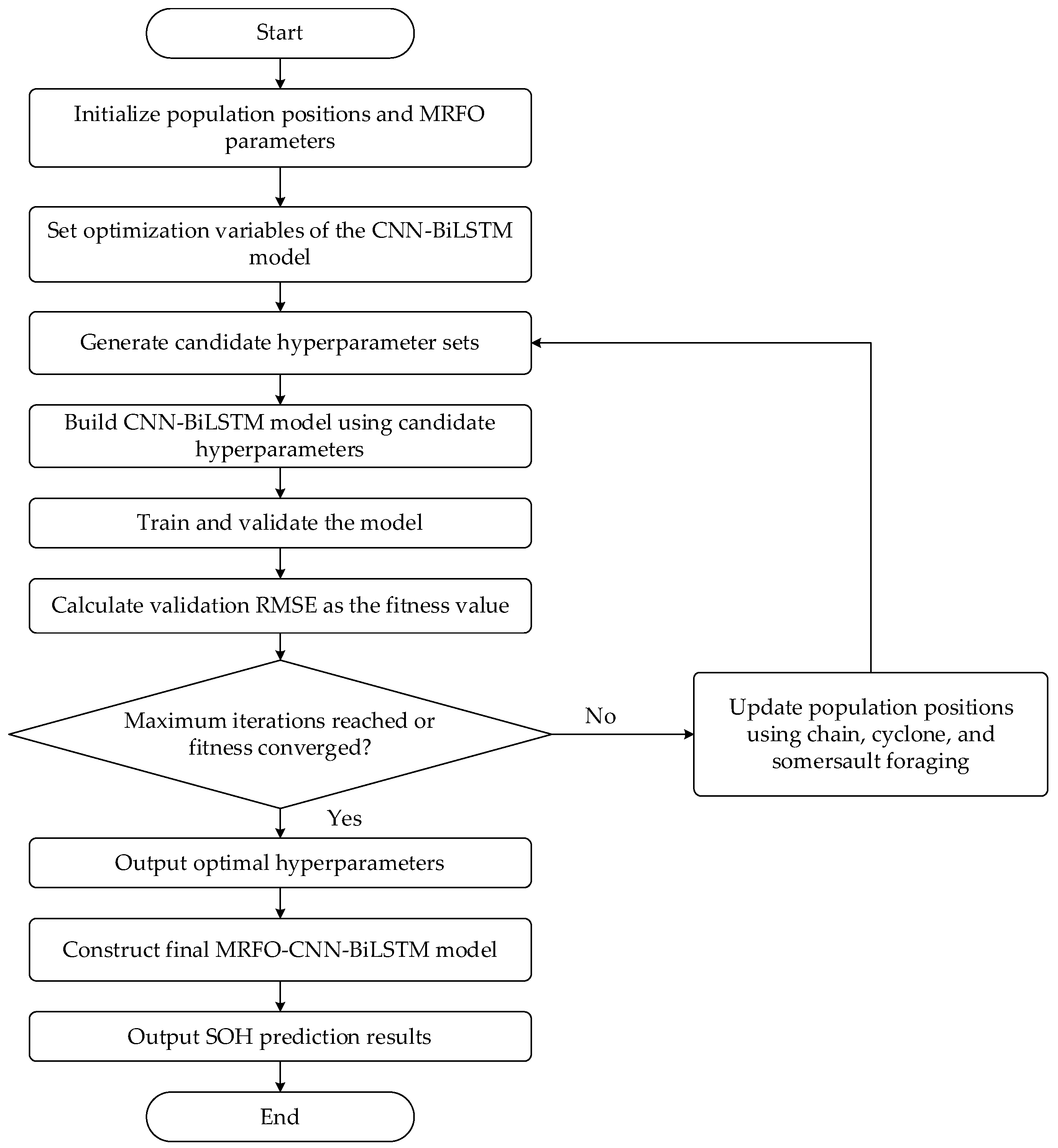
In the proposed optimization process, each individual in the MRFO population represents a candidate hyperparameter combination. For each candidate hyperparameter configuration, the CNN-BiLSTM model is trained and evaluated, and the validation RMSE is taken as the optimization objective. The manta ray population has subsequently evolved chain foraging, cyclone foraging, and somersault foraging strategies. This search procedure is repeated until the preset iteration limit is satisfied or the objective value becomes stable. The overall optimization workflow is illustrated in Figure 5.

Let the hyperparameter vector to be optimized be defined as

$$H=\left[n_{c1},n_{c2},n_h,\alpha ,p\right]$$

(16)

where $n_{c1}$ and $n_{c2}$ are the numbers of convolution kernels in the two convolutional layers, respectively; $n_h$ is the number of BiLSTM hidden units; $\alpha$ is the initial learning rate; and $p$ is the dropout rate. During MRFO, the RMSE calculated on the validation set is used to evaluate each candidate solution. The hyperparameter search is performed by repeatedly adjusting the positions of population members until a better parameter combination is obtained. The optimization objective can be expressed as

$$\min F(H)=\sqrt{{\displaystyle \frac{1}{N}}{\displaystyle \sum _{i=1}^N}{\left(y_i-{\widehat{y}}_i\right)}^2}$$

(17)

where $y_i$ and ${\widehat{y}}_i$ correspond to the measured and predicted SOH values of the i-th sample, respectively, while $N$ is the size of the validation dataset.

During the iterative process of MRFO, the population size, maximum number of iterations, and individual position parameters are first initialized. Then, the model error corresponding to each candidate hyperparameter combination is calculated and used as the fitness value. Next, the individual positions are updated according to the chain foraging, cyclone foraging, and somersault foraging mechanisms. The optimization terminates when either the maximum iteration number is satisfied or the fitness criterion reaches convergence, after which the optimal hyperparameter set is selected. Among them, chain foraging is used to enhance information transfer among population individuals, cyclone foraging is used to improve the search ability in the global optimal region, and somersault foraging is used to further perform fine optimization around the optimal solution.

The weighted fused feature matrix $Z$, together with the corresponding SOH labels, is partitioned into training, validation, and test datasets before model training. The training data are used for parameter updating, the validation data guide the selection of hyperparameter combinations during MRFO, and the test data are employed only to evaluate the final prediction performance. After the optimal hyperparameters are obtained, the CNN-BiLSTM model is reconstructed with these settings and trained using the Adam optimizer. Dropout is introduced to reduce overfitting. Finally, the optimized model is used to predict SOH on the test dataset.

To improve the reproducibility of the proposed method, the model input settings, dataset partition strategy, and MRFO hyperparameter optimization settings are summarized in

Table 4. Model input, dataset partition, and MRFO hyperparameter settings.

Category	Item	Setting/Range	Optimized Value
Input/output setting	Input feature	Weighted fused 11-HF matrix	—
	Input dimension	n × 11	—
	Output	SOH value	—
Main experiment	Training/validation cell	CS2-38	—
	Test cells	CS2-35, CS2-36, and CS2-37	—
	Training/validation ratio	8:2	—
MRFO hyperparameter optimization	Number of filters in Conv1	8–64	32
	Number of filters in Conv2	8–128	64
	Number of BiLSTM hidden units	16–128	64
	Initial learning rate	0.0001–0.01	0.0012
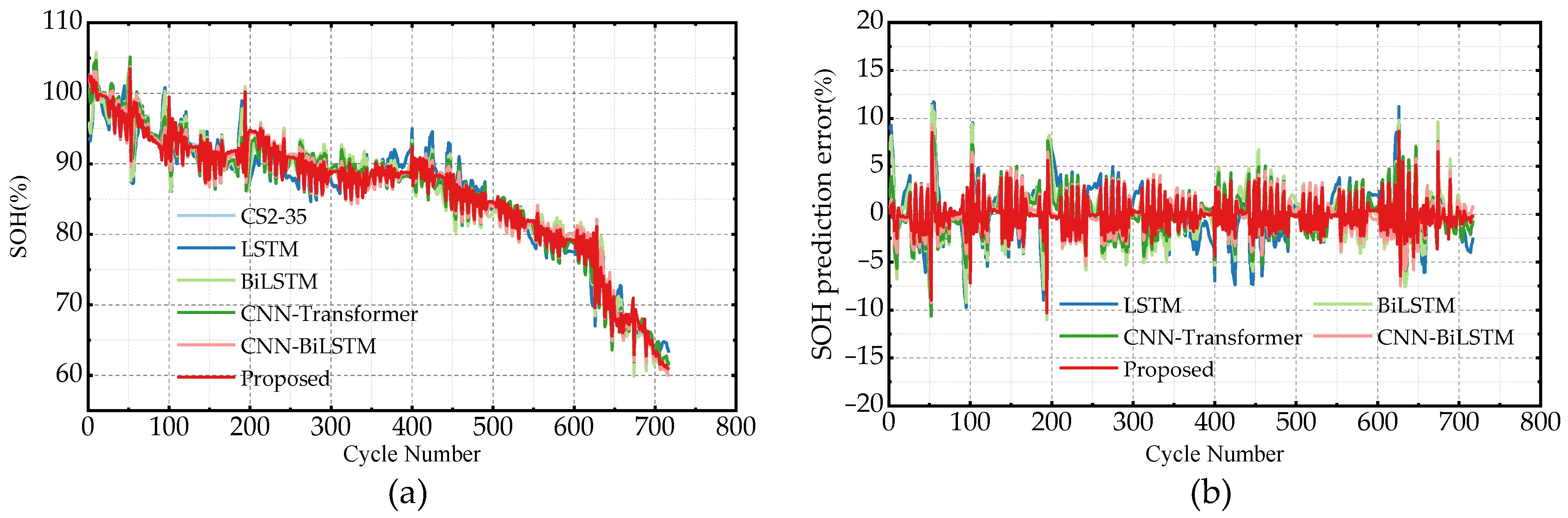
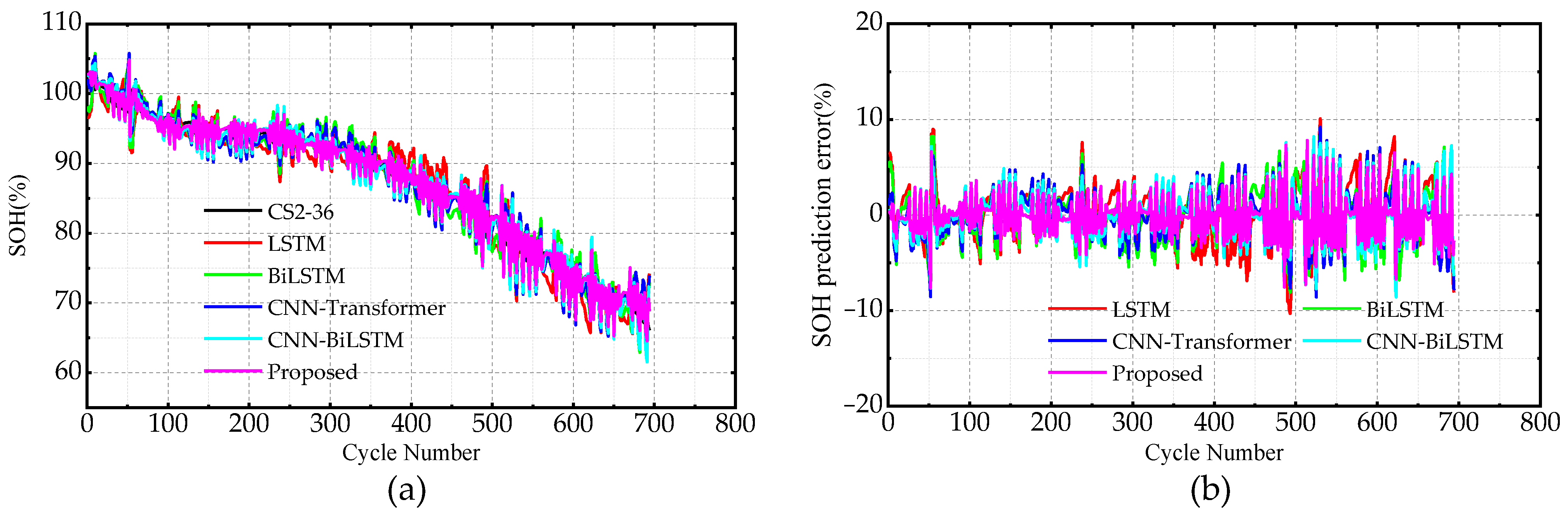
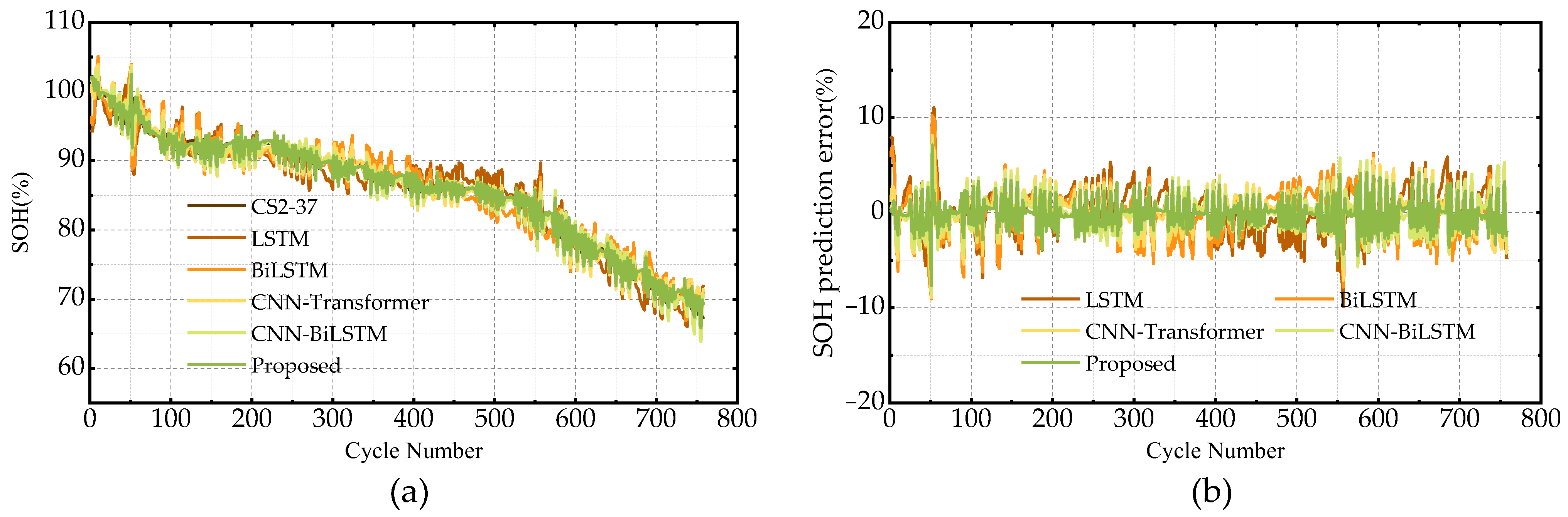
	Dropout rate	0.1–0.5	0.20

. In the main experiment, CS2-38 is used for training and validation, while CS2-35, CS2-36, and CS2-37 are used as independent test cells. In addition, leave-one-cell-out cross-validation is further introduced to evaluate the cross-cell generalization ability of the proposed method under different training-test partitions.

4. Experimental Results and Analysis

4.1. Evaluation Metrics

To comprehensively assess the prediction results, MAE, MAPE, MSE, RMSE, and R² are selected as evaluation indicators. Among them, the error-based metrics reflect the deviation between predicted and actual SOH values, while R² characterizes the fitting degree of the model. Their calculation formulas are as follows:

$$MAE={\displaystyle \frac{1}{n}}{\displaystyle \sum _{i=1}^n}\left|y_i-{\widehat{y}}_i\right|$$

(18)

$$\mathrm{MAPE}={\displaystyle \frac{1}{n}}{\displaystyle \sum _{i=1}^n}\left|{\displaystyle \frac{y_i-{\widehat{y}}_i}{y_i}}\right|\times 100\%$$

(19)

$$MSE={\displaystyle \frac{1}{n}}\sum ^n{\left(y_i-{\widehat{y}}_i\right)}^2$$

(20)

$$RMSE=\sqrt{{\displaystyle \frac{1}{n}}{\displaystyle \sum _{i=1}^n}{\left(y_i-{\widehat{y}}_i\right)}^2}$$

(21)

$$R^2=1-{\displaystyle \frac{{\displaystyle \sum _{i=1}^n}{\left(y_i-{\widehat{y}}_i\right)}^2}{{\displaystyle \sum _{i=1}^n}{\left(y_i-\overline{y}\right)}^2}}$$

(22)

4.2. Experimental Results Based on the CALCE Dataset

4.2.1. Performance Comparison of Different Prediction Models

To evaluate the cross-cell prediction ability of the proposed MRFO-CNN-BiLSTM model, experiments are carried out on the CALCE dataset. CS2-38 is used for model training, while CS2-35, CS2-36, and CS2-37 are used as test batteries. Since these cells show different degradation trajectories, local capacity regeneration, and decline rates, they can be used to examine the adaptability of the model under different aging patterns. LSTM, BiLSTM, CNN-Transformer, CNN-BiLSTM, and MRFO-CNN-BiLSTM are compared under the same experimental setting. The prediction curves and errors are shown in Figure 6, Figure 7 and Figure 8, the statistical comparison results are presented in Figure 9, and the detailed evaluation metrics are listed in

Table 5. Prediction evaluation metrics of different models on the test sets of the CALCE dataset.

Battery No.	Model	MAE/%	MAPE/%	MSE/%	RMSE/%	R2
CS2-35	LSTM	2.519	2.936	0.103	3.205	0.871
	BiLSTM	2.223	2.581	0.086	2.933	0.892
	CNN-Transformer	1.949	2.278	0.063	2.508	0.921
	CNN-BiLSTM	1.639	1.917	0.047	2.168	0.941
	Proposed	1.222	1.435	0.031	1.762	0.961
CS2-36	LSTM	2.623	3.120	0.103	3.202	0.885
	BiLSTM	2.472	2.948	0.091	3.015	0.898
	CNN-Transformer	2.226	2.663	0.078	2.785	0.913
	CNN-BiLSTM	2.019	2.420	0.067	2.586	0.925
	Proposed	1.520	1.824	0.044	2.090	0.951
CS2-37	LSTM	2.248	2.643	0.078	2.796	0.875
	BiLSTM	2.131	2.510	0.070	2.647	0.888
	CNN-Transformer	1.782	2.108	0.048	2.195	0.923
	CNN-BiLSTM	1.619	1.918	0.041	2.016	0.935
	Proposed	1.134	1.345	0.023	1.521	0.963

.

Figure 6, Figure 7 and Figure 8 show that all comparison models can roughly follow the overall SOH decreasing trend. However, their tracking ability differs when the SOH curve contains local fluctuations, capacity regeneration, or a rapid decline in the later cycles. The proposed MRFO-CNN-BiLSTM model shows closer agreement with the true SOH curves on the three test batteries. This advantage indicates that the fused HF provides effective degradation information, while the CNN-BiLSTM structure further improves the representation of local feature interactions and temporal evolution.

The quantitative results in Table 5 further confirm the prediction advantage of the proposed model. For CS2-35, the MAE, MAPE, MSE, RMSE, and R² are 1.222%, 1.435%, 0.031%, 1.762%, and 0.961, respectively. For CS2-36, the corresponding values are 1.520%, 1.824%, 0.044%, 2.090%, and 0.951. For CS2-37, they are 1.134%, 1.345%, 0.023%, 1.521%, and 0.963. Compared with LSTM, BiLSTM, CNN-Transformer, and CNN-BiLSTM, the proposed model gives the lowest error values on all three test batteries, and all R² values are higher than 0.95. The above results suggest that the proposed model achieves a closer fit to the battery SOH degradation trajectory.

To further evaluate the cross-cell generalization ability of the proposed method, leave-one-cell-out cross-validation is conducted. In each round, one cell is used as the independent test cell, while the remaining three cells are used for model training and validation. This validation strategy reduces the dependence of the evaluation results on a single training-test partition and provides a more comprehensive assessment of the model under different cell degradation trajectories. The corresponding results are shown in

Table 6. Leave-one-cell-out cross-validation results.

Round	Training/Validation Cells	Test Cell	MAE/%	MAPE/%	MSE/%	RMSE/%	R2
1	CS2-36, CS2-37, and CS2-38	CS2-35	1.185	1.392	0.029	1.704	0.964
2	CS2-35, CS2-37, and CS2-38	CS2-36	1.463	1.755	0.041	2.025	0.954
3	CS2-35, CS2-36, and CS2-38	CS2-37	1.112	1.319	0.022	1.483	0.966
4	CS2-35, CS2-36, and CS2-37	CS2-38	1.376	1.641	0.037	1.921	0.957
Average	—	—	1.284	1.527	0.032	1.783	0.960

.

As shown in Table 6, the proposed model maintains relatively stable prediction performance under different test-cell settings. The average MAE, MAPE, MSE, RMSE, and R² are 1.284%, 1.527%, 0.032%, 1.783%, and 0.960, respectively. These results indicate that the proposed method has a certain cross-cell generalization capability within the CALCE dataset.

4.2.2. Ablation Experiment

To examine the effect of HF weighting on SOH prediction, an ablation study is conducted under the same model structure, data partition, MRFO settings, and evaluation metrics. Five input strategies are compared: unweighted 11-HF, Weighted Top-3 HF, Weighted Top-5 HF, Weighted Top-7 HF, and Weighted 11-HF. In the unweighted strategy, all normalized HF are directly used as model inputs. In the weighted strategies, HF are weighted according to their Pearson correlations with SOH, and different numbers of HF are selected to form the model inputs. Figure 10 presents the SOH prediction results, Figure 11 compares the average performance of different strategies, and

Table 7. SOH prediction performance under different HF fusion strategies on CS2-35, CS2-36, and CS2-37.

Battery No.	HF Fusion Strategy	MAE/%	MAPE/%	MSE/%	RMSE/%	R2
CS2-35	Unweighted 11-HF	1.486	1.762	0.046	2.142	0.944
	Weighted Top-3 HF	1.802	2.128	0.061	2.471	0.925
	Weighted Top-5 HF	1.625	1.921	0.052	2.287	0.936
	Weighted Top-7 HF	1.414	1.666	0.041	2.016	0.952
	Weighted 11-HF	1.222	1.435	0.031	1.762	0.961
CS2-36	Unweighted 11-HF	1.781	2.143	0.059	2.423	0.934
	Weighted Top-3 HF	2.084	2.496	0.076	2.761	0.912
	Weighted Top-5 HF	1.862	2.236	0.065	2.540	0.927
	Weighted Top-7 HF	1.684	2.017	0.053	2.309	0.941
	Weighted 11-HF	1.520	1.824	0.044	2.090	0.951
CS2-37	Unweighted 11-HF	1.402	1.653	0.041	2.034	0.948
	Weighted Top-3 HF	1.738	2.052	0.057	2.385	0.928
	Weighted Top-5 HF	1.512	1.790	0.046	2.156	0.943
	Weighted Top-7 HF	1.306	1.545	0.035	1.872	0.957
	Weighted 11-HF	1.134	1.345	0.023	1.521	0.963

summarizes the detailed evaluation metrics.

Figure 10 shows that different fusion strategies can follow the main SOH degradation trend, but their performance differs in local fluctuation regions and rapid degradation stages. Compared with unweighted 11-HF, Weighted 11-HF gives prediction curves closer to the true SOH curves, indicating that correlation-based weighting helps strengthen the contribution of more informative HF. In addition, the prediction performance improves when the number of weighted HF increases from Top-3 to Top-5, Top-7, and all 11 HF. This suggests that low-weight HF still contains useful supplementary degradation information.

According to Figure 11 and Table 7, Weighted 11-HF achieves better overall performance on the three test batteries. For CS2-35, CS2-36, and CS2-37, the MAE values of Weighted 11-HF are 1.222%, 1.520%, and 1.134%, respectively; the RMSE values are 1.762%, 2.090%, and 1.521%, respectively; and the R² values are 0.961, 0.951, and 0.963, respectively. These results show that the proposed HF-weighted fusion strategy can retain multidimensional degradation information while emphasizing highly correlated features, thereby improving the accuracy and stability of SOH prediction.

To further analyze the independent contribution of each module in the proposed framework, a module-level ablation experiment is conducted. Different model variants are constructed by removing or replacing specific modules in the complete model. The Without MRFO variant denotes the CNN-BiLSTM model without MRFO-based hyperparameter optimization, which is used to evaluate the contribution of MRFO. The Without CNN variant denotes the MRFO-BiLSTM model without convolutional layers, which is used to evaluate the role of local feature extraction. The Without BiLSTM variant denotes the MRFO-CNN-LSTM model in which BiLSTM is replaced by unidirectional LSTM, which is used to evaluate the effect of bidirectional temporal modeling. The complete model is the proposed MRFO-CNN-BiLSTM method. The corresponding results are shown in

Table 8. Module-level ablation results of the proposed model.

Model Variant	MAE/%	MAPE/%	MSE/%	RMSE/%	R2
Without MRFO	1.895	2.247	0.061	2.470	0.923
Without CNN	1.698	2.013	0.049	2.214	0.938
Without BiLSTM	1.621	1.927	0.046	2.138	0.943
Proposed	1.292	1.535	0.032	1.791	0.958

.

As shown in Table 8, removing or replacing any module from the complete framework leads to a degradation in prediction performance. Compared with the Without MRFO variant, the proposed model achieves lower error values, indicating that MRFO-based hyperparameter optimization helps improve model performance and reduce the influence of empirical parameter selection. Compared with the without CNN variant, the complete model obtains better prediction results, which demonstrates that the convolutional layers are effective in extracting local relationships among multidimensional HFs. In addition, the proposed model outperforms the Without BiLSTM variant, indicating that bidirectional temporal modeling is beneficial for capturing the SOH degradation trend. Overall, the module-level ablation results further verify the independent contributions of MRFO, CNN, and BiLSTM in the proposed framework.

5. Conclusions

Aiming at the problem that a single feature is difficult to fully characterize the SOH evolution of lithium-ion batteries during aging, this paper proposes an SOH prediction method based on multidimensional HF weighted fusion and MRFO-CNN-BiLSTM and verifies it on the CALCE dataset. The main conclusions are as follows.

(1)

The 11 HFs extracted from multiple dimensions, including charge–discharge duration, charging area, IC, voltage change rate, and time ratio, can characterize battery degradation information from different perspectives. The weighted fusion method based on Pearson correlation coefficients can highlight the contributions of highly correlated HF while retaining the supplementary degradation information contained in low-correlation HF, providing effective inputs for SOH prediction.

(2)

By combining CNN for local feature extraction and BiLSTM for forward–backward temporal dependency modeling, the MRFO-CNN-BiLSTM model can effectively characterize battery degradation patterns. With MRFO-assisted hyperparameter tuning, the model obtains R² values higher than 0.95 on the CS2-35, CS2-36, and CS2-37 test batteries.

(3)

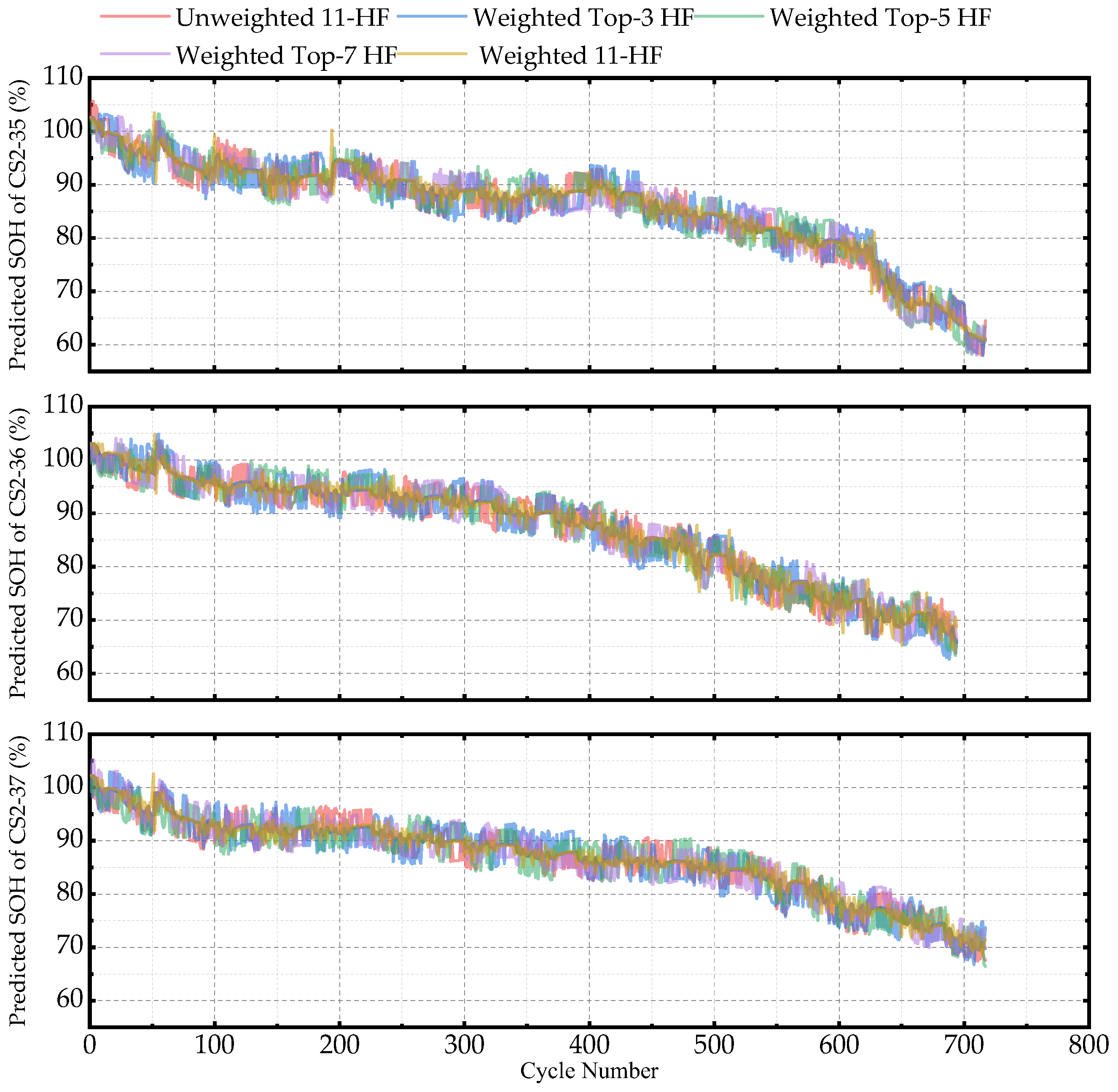
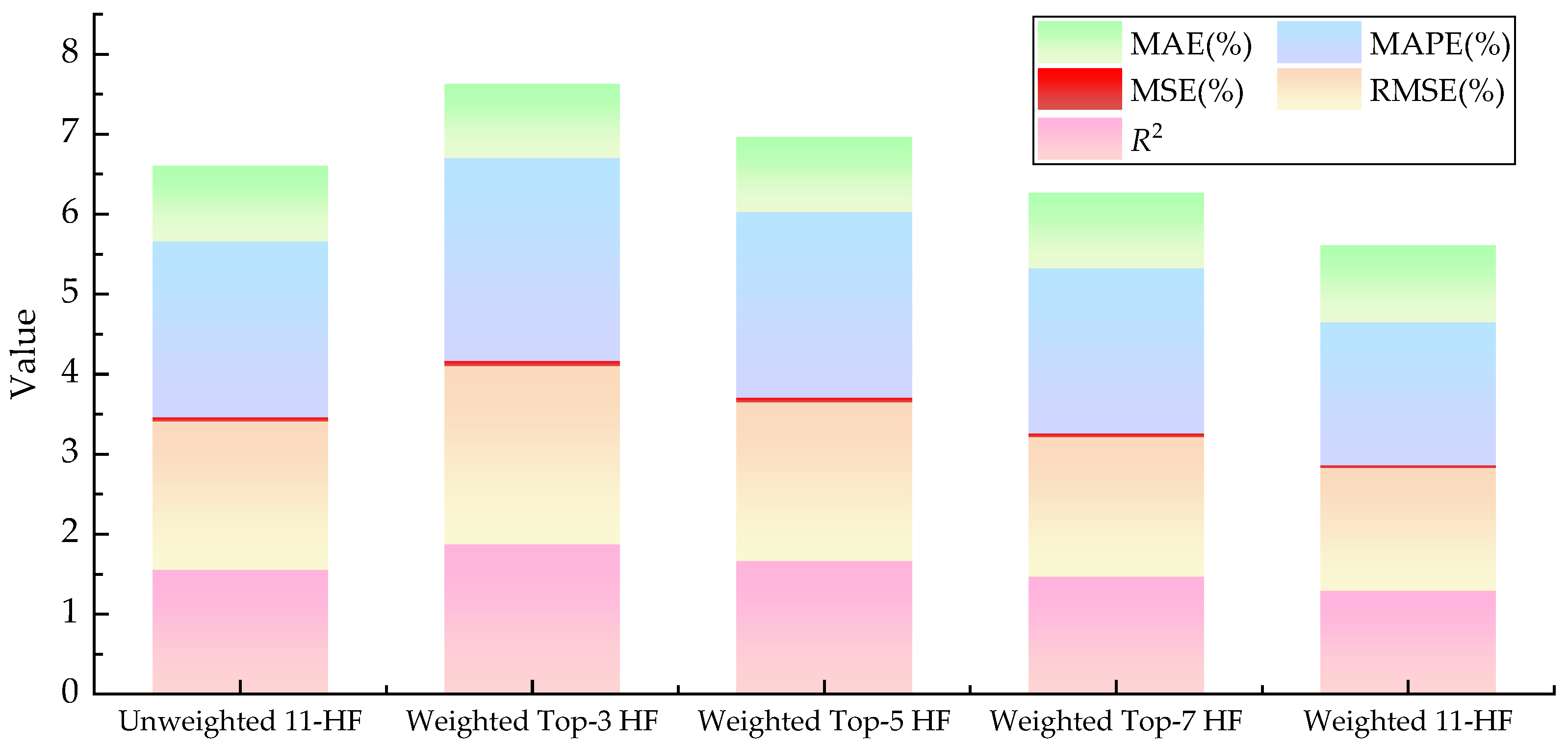
The ablation experiment on HF fusion strategies shows that Weighted 11-HF generally outperforms unweighted 11-HF, Weighted Top-3 HF, Weighted Top-5 HF, and Weighted Top-7 HF. The weighted fusion of all 11 HF can make fuller use of multidimensional degradation information and improve the accuracy and stability of SOH prediction.

It should be noted that the present method mainly relies on complete or nearly complete charge–discharge cycle data. Therefore, it is more suitable for standard laboratory cycle data or application scenarios where complete charging information can be obtained. Future work will further investigate SOH prediction under partial charging segments, different temperatures, different charge–discharge rates, different battery types, and practical BMS operating conditions. In addition, fast electrochemical features such as EIS-related indicators, nonlinear feature weighting strategies, attention mechanisms, and uncertainty estimation methods will be considered to further improve the adaptability, prediction accuracy, and safety-oriented reliability of the proposed framework.