An Adaptive Neuro-Fuzzy Fractional-Order PID Controller for Energy-Efficient Tracking of a 2-DOF Hip–Knee Lower-Limb Exoskeleton

Abstract

For safe and efficient human–robot interaction, lower-limb exoskeletons used for assistance and rehabilitation need to be precisely and energy-efficiently controlled. By creating an adaptive neuro-fuzzy fractional-order PID (ANFIS-FOPID) controller, this project seeks to improve tracking accuracy, robustness, and energy efficiency in a two-degree-of-freedom hip–knee exoskeleton. The Euler–Lagrange formulation is used to derive a nonlinear dynamic model, and a Lyapunov-based stability analysis is used to show that the closed-loop system remains uniformly ultimately bounded under disturbances and parameter uncertainties. The suggested controller performs noticeably better than traditional PID and fixed-parameter FOPID controllers, according to numerical simulations conducted under both normal and perturbed conditions. The ANFIS FOPID achieves root mean square errors below 0.028 rad and lowers the integral absolute errors at the hip and knee joints to 0.1454 and 0.1480, as opposed to 0.3496–0.3712 for PID controllers. Under ±10% parameter uncertainty, the total control-energy proxy drops from 2870.0 (PID) to 936.25, a 67.4% decrease, and stays at 1587.93. Statistically significant variations in energy consumption are confirmed by one-way ANOVA (p < 10⁻¹⁷⁶). Large effect sizes are found (η² = 0.237–0.314). These results demonstrate the superior tracking performance, robustness, and energy efficiency of the ANFIS-FOPID controller. The results set a quantitative standard for future experimental validation and hardware-in-the-loop implementation, despite being based on high-fidelity simulations.

1. Introduction

Exoskeletons for the lower limbs have proven to be a significant technology in the fields of rehabilitation engineering, assistive mobility, and human performance enhancement [1]. These robotic systems are designed to have mechanical contact with the human body, which helps support the joints, including the hip, knee, and ankle, which are the most critical. They find application in numerous areas, such as stroke and spinal cord injury rehabilitation, industrial load handling, military training, and assisting the elderly population to move around [1,2,3]. Although there has been a lot of advancement in their mechanical design, sensing, and actuation, control has been one of the greatest challenges in the development of exoskeletons [3,4]. In comparison with conventional industrial robots, lower-limb exoskeletons collaborate directly with humans, and this fact poses a number of special challenges [5]. Human–exoskeleton systems are extremely nonlinear, as they involve interactions between different links, the force of gravity, and joint coupling [6]. Even in the simplest two-dimensional models, hip and knee dynamics are strongly coupled by inertia and Coriolis forces. The human body is prone to time-varying uncertainties; mass distribution, joint stiffness, and damping are just a few examples of parameters that differ among individuals and are time-varying in an individual user.

In addition, the activation of the muscles generates unmodeled forces, which are perturbations of the robotic system [6,7]. It is vital that the most attention should be paid to the safety and comfort of the subject wearing an exoskeleton; to be more precise, excessively large or excessively jerky actuator torques may lead to an unpleasant or exhausting experience, or even physical harm [8]. Hence, the precision of control actions is as important as the precision of tracking [9]. Another important aspect is the energy efficiency of the system, since several exoskeletons have batteries [10]. The direct effects of increased control effort are a higher power consumption, reduced operating times, actuator heating, and accelerated part wear [10,11]. Thus, energy-saving control measures are crucial to apply in practice. These threats necessitate control systems that are accurate, robust, flexible, and economical. The most-used control methods in robotics and mechatronic systems are proportional–integral–derivative (PID) controllers. This is attributed to the fact that they are easy to install and do not need a lot of computing power [12]. Lower-limb exoskeletons typically use PID controllers at the joint level to walk according to a desired pattern. These models tend to be founded on clinical or biomechanical data [13,14]. Nevertheless, classical PID control has various recognized limitations in its implementation in exoskeleton systems, such as fixed gains (once tuned, PID gains will always be constant and the controller will ignore system changes and operation conditions) [15] and aggressive torque behavior (high proportional and derivative gains are commonly needed to obtain good tracking performance, and result in oscillatory torque profiles and high energy consumption) [13]. The robustness of PID controllers is limited and they usually fail when responding to large uncertainties, disturbances, or parameter variations [13,15]. As a result, the efficacy of PID control is compromised in conditions requiring energy efficiency, robustness, and adaptability when none of these factors can be overlooked, even though PID control can be used to provide satisfactory tracking in ideal conditions [11].

Fractional-order control has attracted a lot of attention in the past 20 years as a development of conventional integer-order control [16]. The FOPID controller is a continuation of the PID controller, which allows the integral and derivative orders to take non-whole values [16]. In the traditional FOPID controller, there are five parameters to be tuned [17]. The main advantage of fractional-order proportional–integral–derivative (FOPID) control is the tuning flexibility. Fractional orders add extra degrees of freedom and therefore more accurate control of the system dynamics is attained [17]. When correctly tuned, FOPID controllers can reduce overshoot and oscillations and thus provide a better tradeoff between tracking performance and smoothness, as compared to traditional PID controls [16,18]. On the other hand, FOPID controllers are limited to constant parameter values, which hinders their capacity to change with changing working conditions [19]. It is not straightforward to adjust five parameters to obtain the most desirable values, particularly with nonlinear systems such as exoskeletons [19,20]. Consequently, adaptive and intelligent control techniques have become a topic of interest in exoskeletons to address the shortcomings of controllers with constant gains. These methods aim to dynamically vary the control parameters based on real-time feedback to enhance robustness as well as overall performance. Neuro-fuzzy systems have gained relevance in intelligent systems since they integrate the learning capabilities of neural networks with the interpretability of fuzzy logic [21]. Adaptive neuro-fuzzy inference systems (ANFISs) have a special application since they are also able to model the nonlinearity of the relationship, yet maintain a structured rule-based model [21].

ANFIS-based techniques have been employed in exoskeleton control to regulate joint impedance parameters and minimize modeling uncertainties as well as optimize PID gains in real-time [22,23]. Most modern ANFIS-based controllers are integer-order PID controllers, however, and thus do not take advantage of the advantages of fractional-order control [24,25]. Fractional-order control and intelligent adaptation have been individually applied to robotic systems and exoskeleton systems; however, there are limited studies on the systematic integration of these control systems to achieve energy-efficient control of exoskeletons. In particular, dynamic changes in both FOPID gains and fractional orders, based on a neuro-fuzzy mechanism, has not been fully examined with reference to lower-limb exoskeletons. In addition, while most studies mention the accuracy of tracking or its robustness, the energy consumption of the controller is still frequently ignored or analyzed only qualitatively. Since energy efficiency is a practical issue in wearable robotics, it is necessary to provide a stringent quantitative and statistical analysis. The study pursues three primary objectives:

• To develop a nonlinear dynamic model of a 2-DOF hip–knee exoskeleton using a Euler–Lagrange formulation, incorporating friction and disturbance effects.
• To design an adaptive neuro-fuzzy fractional-order PID controller capable of real-time gain and fractional-order adaptation.
• To evaluate the tracking precision, robustness, and controller energy consumption under nominal and uncertain operating conditions.

In conclusion, this work is situated at the nexus of nonlinear control-oriented modeling and assistive lower-limb rehabilitation applications. The exoskeleton is viewed as a dynamic human–machine system, and the structure required for sophisticated control synthesis is provided by the modeling framework that is obtained using the Euler–Lagrange formulation. Building on this framework, the suggested ANFIS–FOPID controller is created to improve trajectory accuracy and lower control energy usage in both nominal and unpredictable scenarios. The overall contributions made by this study include:

• Development of an adaptive neuro-fuzzy inference system (ANFIS)-driven fractional-order PID (FOPID) controller. This controller is designed to adjust both control gains and fractional orders simultaneously. The purpose is to control a nonlinear 2-DOF hip–knee lower-limb exoskeleton.
• A thorough quantitative assessment of tracking accuracy and controller energy use was conducted, considering normal conditions, external disturbances, and uncertainties in system parameters.
• To statistically confirm the energy efficiency of the control, we used a one-way ANOVA and an analysis of effect size.
• An analysis of boundedness, based on Lyapunov methods, is used to ensure the stability of the adaptive fractional-order control framework.

2. System Modeling

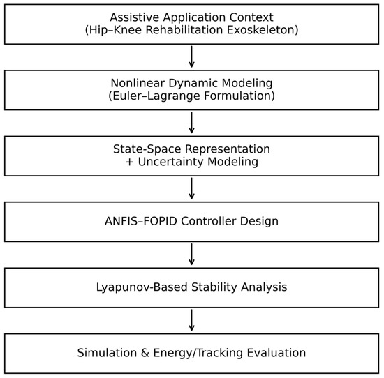
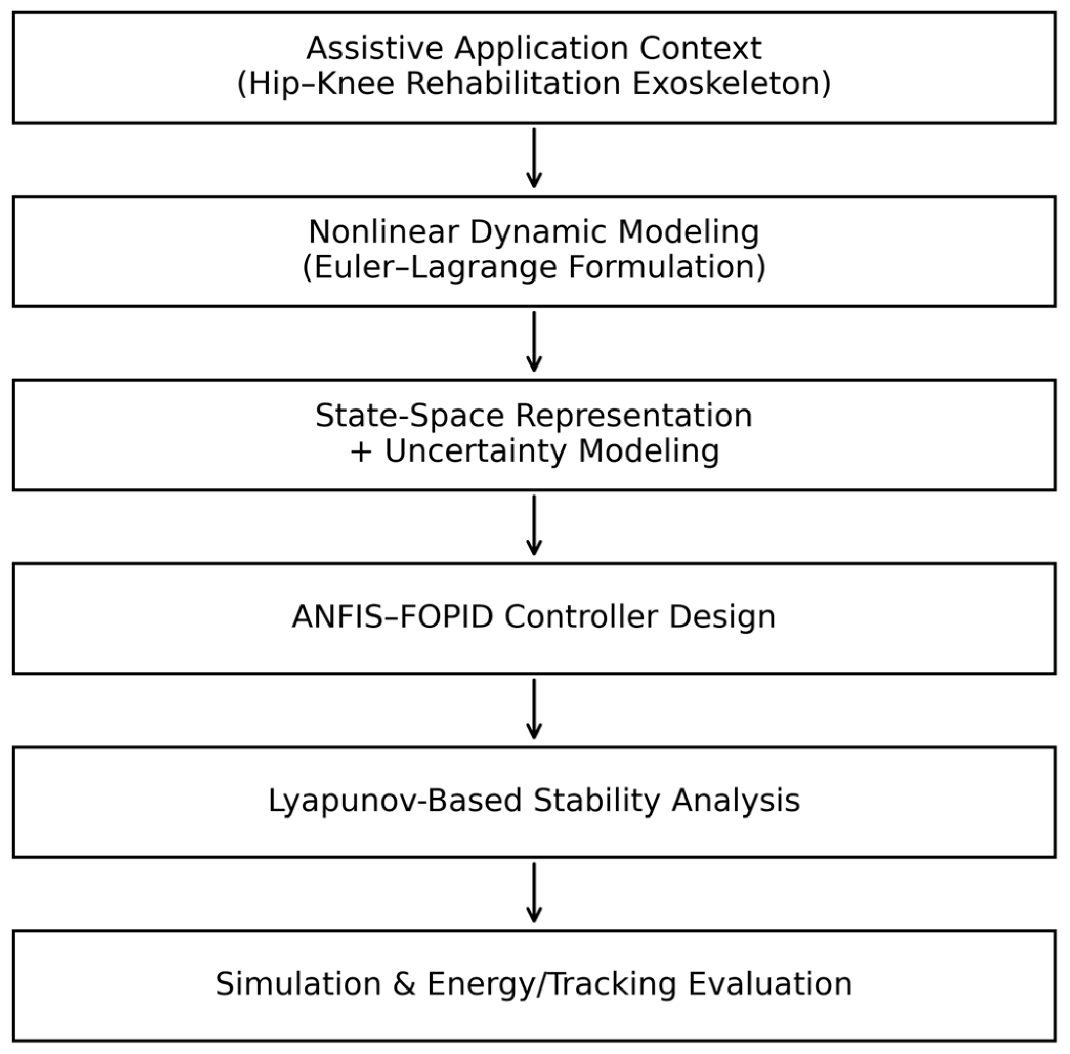
In the section below, a nonlinear dynamic model of the 2-DOF hip–knee lower-limb exoskeleton is given in detail. A model is constructed using Lagrangian mechanics, which is highly applicable to robotic systems with many links and joint dynamics that are interlinked can be compactly represented. We obtain explicit equations of the inertia matrix, Coriolis, centrifugal terms, and the gravity vector. Figure 1 shows a summary of the proposed study’s methodological framework. This helps make the structure clearer and gives an overview of the research workflow. The research advances from the context of assistive exoskeleton applications to nonlinear dynamic modeling, controller synthesis, stability validation, and performance assessment. This structured flow shows how the modeling framework helps the work’s goals of being control-oriented.

Modeling Assumptions

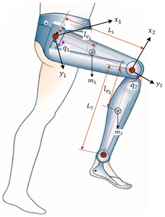
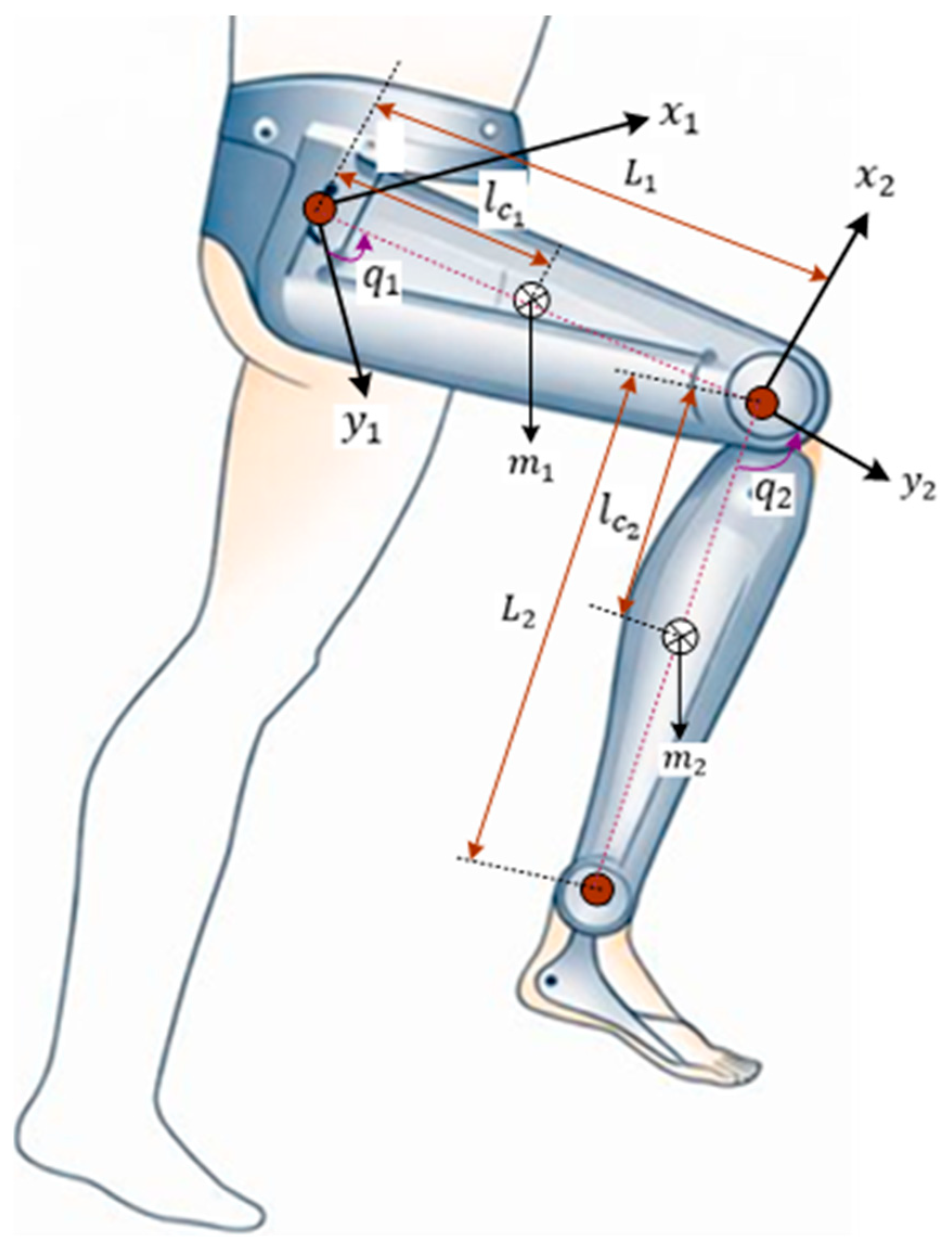
To obtain the required analytical mathematical model of the lower limb considered in this work, we use following modeling assumptions: 1. The exoskeleton is treated as a rigid body with a constant mass and moment of inertia at each of the links. 2. Movement is limited to the sagittal plane; movements in other planes are not available. 3. The joints used are ideal revolute joints, without backlash and compliance. 4. There are no actuator dynamics; actuators are assumed to exert commanded torques instantly. 5. Joint friction is modeled as viscous friction, and it is included as a form of additive damping. 6. The interaction forces between the human being and exoskeleton are affected as a bounded disturbance, and they are not explicitly modeled. These are standard assumptions in control-based exoskeleton modeling and are used as a strong basis in the design and analysis of controllers. In line with standard procedure in lower-limb exoskeleton control studies, the effects of human–exoskeleton interaction forces are included as bounded external disturbances even though they are not explicitly modeled.

Table 1. Geometric and mass properties of the 2-DOF hip–knee exoskeleton model (sagittal plane).

Symbol	Description	Value and Unit
$M_b$	Body mass	75 kg
$H$	Body height	1.75 m
$L_1$	Thigh length (hip to knee)	0.43 m
$L_2$	Shank length (knee to ankle)	0.43 m
$m_1$	Thigh segment mass	7.5 kg
$m_2$	Shank segment mass	3.5 kg
$l_{c1}$	Thigh COM distance from the hip	0.19 m
$l_{c2}$	Shank COM distance from the knee	0.19 m
$I_1$	Thigh inertia about COM (planar)	$0.13 \mathrm{kg}·{\mathrm{m}}^2$
$I_2$	Shank inertia about COM (planar)	$0.06 \mathrm{kg}·{\mathrm{m}}^2$
$g$	Gravity	$9.81 \mathrm{m}/{\mathrm{s}}^2$
$b_1$	Hip viscous friction	0.8 N·m·s/rad
$b_2$	Knee viscous friction	0.6 N·m·s/rad
${\tau }_{1,\mathrm{m}\mathrm{a}\mathrm{x}}$	Hip torque limit	60 N·m
${\tau }_{2,\mathrm{m}\mathrm{a}\mathrm{x}}$	Knee torque limit	60 N·m

shows the system parameters utilized. Figure 2 represents a schematic diagram of a 2-DOF lower-limb exoskeleton.

Let $q=[q_1 q_2{]}^T$ and $\dot{q}$ be hip and knee angles and velocities, and $\tau =[{\tau }_1 {\tau }_2{]}^T$ the joint torques. The sagittal-plane rigid-body dynamics with viscous friction are [26]:

$$M\left(q\right)\ddot{q}+C\left(q,\dot{q}\right)\dot{q}+G\left(q\right)+B\dot{q}=\tau$$

(1)

$$B=\left[\begin{array}{cc}{b}_1& 0\\ 0& b_2\end{array}\right]$$

(2)

Using the conventional 2-link planar manipulator form (link-2 relative angle $q_2$), the matrices are

$$M\left(q\right)=\left[\begin{array}{cc}{M}_{11}& M_{12}\\ M_{12}& M_{22}\end{array}\right]$$

(3)

where

$$\begin{array}{cc}{M}_{11}& =I_1+I_2+m_1{l}_{c1}^2+m_2\left(L_1^2+l_{c2}^2+2L_1{l}_{c2}\cos q_2\right),\\ M_{12}& =I_2+m_2\left(l_{c2}^2+L_1{l}_{c2}\cos q_2\right)\\ M_{22}& =I_2+m_2{l}_{c2}^2\end{array}$$

Let $h\left(q_2\right)=m_2{L}_1{l}_{c2}\sin q_2$. A common Coriolis/centrifugal matrix is

$$C\left(q,\dot{q}\right)=\left[\begin{array}{cc}-h{\dot{q}}_2& -h\left({\dot{q}}_1+{\dot{q}}_2\right)\\ h{\dot{q}}_1& 0\end{array}\right]$$

(4)

Gravity vector (with $q_1$ absolute and $q_1+q_2$ for link 2):

$$G\left(q\right)=\left[\begin{array}{c}\left(m_1{l}_{c1}+m_2{L}_1)\mathrm{g}\mathrm{c}\mathrm{o}\mathrm{s} q_1+m_2{l}_{c2}\mathrm{g}\mathrm{c}\mathrm{o}\mathrm{s} (q_1+q_2\right)\\ m_2{l}_{c2}\mathrm{gcos} \left(q_1+q_2\right)\end{array}\right]$$

(5)

Substituting the values from Table 1 at $q_2=0$, the numerical mass matrix is

$$M\left(0\right)=\left[\begin{array}{cc}1.80615& 0.47230\\ 0.47230& 0.18635\end{array}\right]$$

(6)

Nonlinear state-space model.

Let the state $x=[q_1 q_2 {\dot{q}}_1 {\dot{q}}_2{]}^T$ and input $u=\tau$. Then,

$$\dot{x}=\left[\begin{array}{c}\dot{q}\\ M(q{)}^{-1}\left(\tau -C\left(q,\dot{q}\right)\dot{q}-G\left(q\right)-B\dot{q}\right)\end{array}\right]$$

(7)

Linearization was done about $\left(q,\dot{q})=(0,0\right),$ and we assumed that the gravity is compensated by a constant feedforward torque $u_0=G\left(q_0\right)$; the small-signal model becomes

$$\delta \dot{x}=A\hspace{0.17em}\delta x+B\hspace{0.17em}\delta u$$

(8)

with

$$A=\left[\begin{array}{cccc}0& 0& 1& 0\\ 0& 0& 0& 1\\ 0& 0& -1.31338& 2.49655\\ 0& 0& 3.32873& -9.54719\end{array}\right],$$

(9)

$$B=\left[\begin{array}{cc}0& 0\\ 0& 0\\ 1.64172& -4.16091\\ -4.16091& 15.91199\end{array}\right]$$

(10)

These values come from $M(0{)}^{-1}$ and viscous friction $B$.

3. Controller Design

This section presents the proposed ANFIS-FOPID controller as applied to the lower-limb 2-DOF hip–knee exoskeleton. The controller aims to achieve three primary objectives, namely, (i) precise tracking of joint trajectories, (ii) robustness to nonlinearities, uncertainties, and disturbances, and (iii) minimization of controller energy consumption. The baseline control structure is an FOPID controller, which is integrated with the ANFIS to vary the controller parameters online.

3.1. Control Objectives and Error Dynamics

Let the desired joint trajectories be defined as

$$q_d\left(t\right)=\left[\begin{array}{c}{q}_{1d}\left(t\right)\\ q_{2d}\left(t\right)\end{array}\right]$$

(11)

where the desired hip- and knee-joint angles are represented as $q_{1d}\left(t\right)$ and $q_{2d}\left(t\right)$, respectively. Thus, the position and velocity errors are defined as

$$e\left(t\right)=q\left(t\right)-q_d\left(t\right),\dot{e}\left(t\right)=\dot{q}\left(t\right)-{\dot{q}}_d\left(t\right).$$

(12)

The objective of control is to achieve $\underset{t\to \mathrm{\infty }}{\lim e\left(t\right)}=0 \mathrm{a}\mathrm{n}\mathrm{d} \underset{t\to \mathrm{\infty }}{\lim \dot{e}\left(t\right)}=0;$ by proper design, the control torques $\tau \left(t\right)$ guarantee smooth control torque and the reduction of energy consumption.

3.2. Baseline Fractional-Order PID Controller

The fractional-order PID controller is an extension of a traditional PID controller, done through the employment of non-integer values as the order of the integral and derivative. The law of FOPID control is defined in each joint, as follows [27]:

$$u\left(t\right)=K_{p}e\left(t\right)+K_i{D}^{-\lambda }e\left(t\right)+K_d{D}^{\mu }e\left(t\right),$$

(13)

where $K_p\in {\mathbb{R}}^{2\times 2}$ is the proportional gain matrix, $K_i\in {\mathbb{R}}^{2\times 2}$ is the integral gain matrix, $K_d\in {\mathbb{R}}^{2\times 2}$ is the derivative gain matrix, $D^{-\lambda }$ denotes a fractional integral operator of order $\lambda \in \left(0,1\right)$, and $D^{\mu }$ denotes a fractional derivative operator of order $\mu \in \left(0,1\right)$.

In the Laplace domain, the FOPID controller can be expressed as [27]

$$U\left(s\right)=\left(K_p+K_i{s}^{-\lambda }+K_d{s}^{\mu }\right)E\left(s\right).$$

(14)

Implementation of Fractional Operators

In realistic applications of digital control, the operators of fractional derivatives are modeled by finite-dimensional rational transfer functions. The Oustaloup recursive approximation is used in this study due to its satisfactory properties of accuracy and stability.

The fractional operator $s^{\alpha }$ over the frequency range $\left[{\omega }_L,{\omega }_H\right]$ is approximated as [27]

$$s^{\alpha }\approx K{\prod }_{k=-N}^N{\displaystyle \frac{s+{\omega }_k^{\prime }}{s+{\omega }_k}},$$

(15)

The approximation order is denoted by N and ${\omega }_k$, and ${\omega }_k^{\prime }$ are frequencies chosen accordingly for the purpose. In order to prevent high-frequency noise amplification and guarantee closed-loop stability, an approximation order and frequency range were chosen. This simplification adds more internal states. The simulation includes these states, which do not modify the fundamental setting of the control law.

3.3. ANFIS-Based Adaptive Tuning Mechanism

To avoid fixed-parameter control issues, an ANFIS is constructed in the FOPID controller. The primary task of the ANFIS is to modify the FOPID parameters depending on the success of the system in real-time tracking. The ANFIS ensures bounded adaptation and real-time feasibility by operating strictly in inference mode during online operation, with all membership functions and rule parameters fixed following offline training.

ANFIS Inputs and Outputs

Although the plant dynamics of the 2-DOF exoskeleton are coupled through the inertia matrix $M(q)$ and Coriolis matrix $C(q,\dot{q})$, the feedback controller was implemented per joint (i.e., joint-wise manner). Precisely, the PID gains are structured as diagonal matrices: $K_p(t)=\mathrm{d}\mathrm{i}\mathrm{a}\mathrm{g}\left(k_{p1}(t),\hspace{0.17em}{k}_{p2}(t)\right),$ $K_i(t)=\mathrm{d}\mathrm{i}\mathrm{a}\mathrm{g}\left(k_{i1}(t),\hspace{0.17em}{k}_{i2}(t)\right),$ and $K_d(t)=\mathrm{d}\mathrm{i}\mathrm{a}\mathrm{g}\left(k_{d1}(t),\hspace{0.17em}{k}_{d2}(t)\right)$. In this manner, each joint has its own independently adapted gain parameters. Likewise, the fractional integral and derivative orders are defined per joint: $\lambda (t)=\mathrm{d}\mathrm{i}\mathrm{a}\mathrm{g}\left({\lambda }_1(t),\hspace{0.17em}{\lambda }_2(t)\right)$ and $\mu (t)=\mathrm{d}\mathrm{i}\mathrm{a}\mathrm{g}\left({\mu }_1(t),\hspace{0.17em}{\mu }_2(t)\right)$.

Accordingly, the ANFIS module produces independent parameter updates for each joint. For joint $i\in \{1,2\}$, the adaptive parameter vector is defined as

$$\Delta {\theta }_i(t)=\left[\begin{array}{c}\Delta k_{pi}(t)\\ \Delta k_{ii}(t)\\ \Delta k_{di}(t)\\ \Delta {\lambda }_i(t)\\ \Delta {\mu }_i(t)\end{array}\right]$$

(16)

The time-varying parameter vector is then expressed as

$${\theta }_i(t)={\theta }_{i0}+\Delta {\theta }_i(t),$$

(17)

where ${\theta }_{i0}$ denotes the initial nominal parameters. For compact notation, the global stacked adaptive vector is defined as $\Delta \Theta (t)=\left[\begin{array}{c}\Delta {\theta }_1(t)\\ \Delta {\theta }_2(t)\end{array}\right]\in {\mathbb{R}}^{10}.$

Dimensional consistency between the adaptive outputs and the joint-wise controller implementation is guaranteed by this formulation.

3.4. Structure of the ANFIS

The ANFIS is employed as a first-order Sugeno-type fuzzy inference system comprising five layers:

Layer 1. Fuzzification: Each input relates to five Gaussian membership functions that match the linguistic terms [28]:

$${\mu }_{A_i}\left(x\right)=\exp \left(-{\displaystyle \frac{(x-c_i{)}^2}{2{\sigma }_i^2}}\right)$$

(18)

Layer 2. Rule Layer: Each node denotes a fuzzy rule, and the firing strength of the $\left(i,j\right)$-th rule is computed as

$$w_{ij}={\mu }_{E_i}\left(x_1\right){\mu }_{D{E}_j}\left(x_2\right).$$

(19)

Layer 3—Normalization: Normalized firing strengths are computed as

$${\overline{w}}_{ij}={\displaystyle \frac{w_{ij}}{\sum _{i,j}{w}_{ij}}}.$$

(20)

Layer 4—Consequent Layer: Each rule outputs a linear function of the inputs:

$$f_{ij}=a_{ij}{x}_1+b_{ij}{x}_2+c_{ij}.$$

(21)

Layer 5—Output Layer: The final ANFIS output is obtained as a weighted sum of all rule outputs:

$$f_{ANFIS}\left(t\right)=\sum _{ij}{\overline{w}}_{ij}{f}_{ij}$$

(22)

3.5. 5 × 5 Fuzzy Rule Base

The ANFIS also uses five functions of its membership to each input, giving it 25 fuzzy rules. One of the common rules is developed as [29]

$$\mathrm{IF} e \mathrm{is} E_i \mathrm{AND} \dot{e} \mathrm{is} D{E}_j \mathrm{THEN} \Delta \theta =f_{ij}$$

(23)

The qualitative structure of the rule base is defined according to control heuristics: high error causes proportional and derivative gains to increase, consistent error causes an increase in integral action, and quick changes in error need a change in derivative gain and fractional order to enhance damping.

3.6. Training of ANFIS

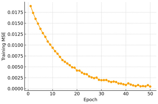
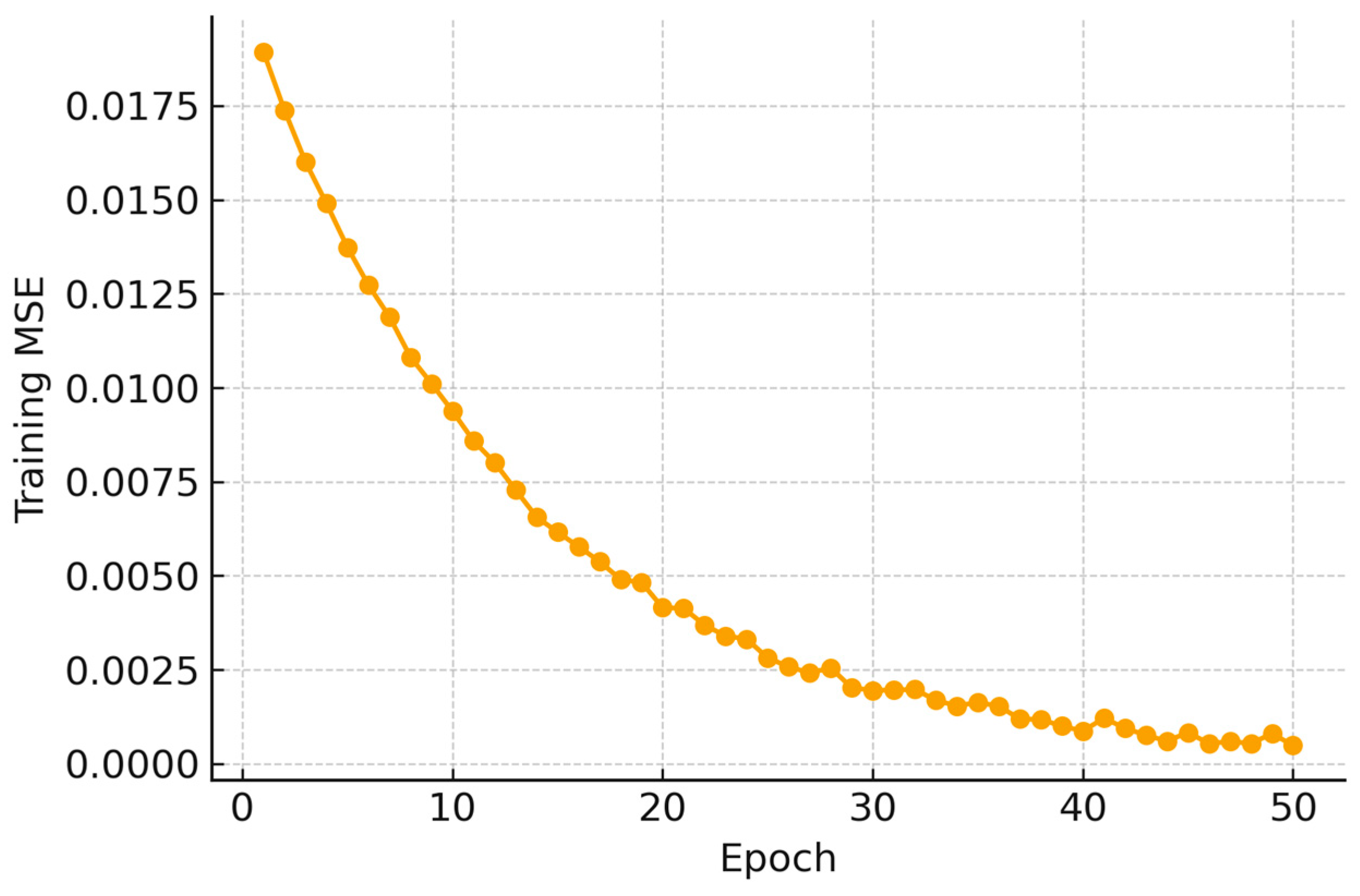
The hybrid training procedure consists of a forward pass (least squares estimation of consequent parameters) and a backward pass, wherein gradient descent updates the membership function parameters. The training data is generated by: simulating joint trajectories with varying disturbances; recording the optimal control corrections; feeding the error + error-rate signals with the desired parameter updates. Training occurs offline. During operation, ANFIS is applied in an inference mode during operation that is computationally lightweight. Figure 3 shows that the ANFIS converges at approximately 50 epochs.

3.7. Combined ANFIS–FOPID Control Law

The final control torque exerted on the exoskeleton joints is expressed as:

$$\tau \left(t\right)=K_p\left(t\right)e\left(t\right)+K_i\left(t\right)D^{-\lambda \left(t\right)}e\left(t\right)+K_d\left(t\right)D^{\mu \left(t\right)}e\left(t\right)+G\left(q\right),$$

(24)

$G\left(q\right)$ is the gravity compensator. This structure combines model-based compensation (gravity) and fractional-order control to achieve better robustness and intelligent adaptation to achieve energy-efficient performance, where $K_p,K_i,K_d$ are the time-varying proportional, integral, and derivative gains, and $\lambda , \mu$ are the fractional orders of the integral and derivative actions, respectively. ANFIS uses these five parameters, which are real-time-generated and can be considered a first-order Sugeno fuzzy model with Gaussian membership functions on the inputs $\left[e_i,{\dot{e}}_i\right]$. Figure 4 shows the architecture of the suggested ANFIS-FOPID controller.

4. Lyapunov-Based Stability Analysis

This section presents a Lyapunov-based stability derivation of the suggested ANFIS-FOPID-controlled 2-DOF lower-limb exoskeleton. The novelty of the use of fractional-order operators, as well as the neuro-fuzzy adaptation, makes it difficult to derive strict asymptotic stability in the classical framework. As a result, the analysis focuses on achieving boundedness, convergence to a compact set, and the ability to withstand disturbances, which are identified as stability guarantees of adaptive and intelligent control systems in wearable robotics. The closed-loop exoskeleton dynamics including modeled viscous friction are expressed as

$$M(q)\ddot{q}+C(q,\dot{q})\dot{q}+G(q)+B\dot{q}=\tau +d(t)$$

(25)

where $B=\mathrm{d}\mathrm{i}\mathrm{a}\mathrm{g}(b_1,b_2)$ represents the viscous friction matrix defined in Table 1. Any unmodeled dynamics (e.g., Coulomb friction, actuator nonlinearities, or interaction forces) are incorporated into the bounded disturbance term $d(t)$.

Let the tracking error be defined as

$$e=q-q_d,\dot{e}=\dot{q}-{\dot{q}}_d,\ddot{e}=\ddot{q}-{\ddot{q}}_d.$$

(26)

Substituting the plant dynamics into the error dynamics yields

$$M(q)\ddot{e}+C(q,\dot{q})\dot{e}+B\dot{e}+K_p(t)e+K_i(t)D^{-\lambda (t)}e+K_d(t)D^{\mu (t)}e=\mathsf{\Phi }(t),$$

(27)

where the lumped bounded term is explicitly defined as

$$\mathsf{\Phi }(t)=d(t)-M(q){\ddot{q}}_d-C(q,\dot{q}){\dot{q}}_d-B{\dot{q}}_d+{\epsilon }_{\mathrm{FO}}(t)+{\epsilon }_{\mathrm{ANFIS}}(t).$$

(28)

where $d(t)$ represents bounded external disturbances, ${\epsilon }_{\mathrm{FO}}(t)$ denotes approximation errors due to fractional-order realization, ${\epsilon }_{\mathrm{ANFIS}}(t)$ represents bounded adaptation imperfections, $q_d, {\dot{q}}_d,$ and ${\ddot{q}}_d$ are assumed smooth and bounded. Therefore, $\mathsf{\Phi }(t)$ is bounded.

The standard properties of robot manipulators used in the analysis include the following [30,31]:

Property 1 (Positive definiteness): The inertia matrix $M\left(q\right)$ is symmetric and uniformly positive definite:

$$m_{\mathrm{m}\mathrm{i}\mathrm{n}}I\le M\left(q\right)\le m_{\mathrm{m}\mathrm{a}\mathrm{x}}I,\forall q$$

(29)

Property 2 (Skew-symmetry): The matrix $\dot{M}\left(q\right)-2C\left(q,\dot{q}\right)$ is skew-symmetric:

$$x^{\mathrm{\top }}\left(\dot{M}-2C\right)x=0,\forall x\in {\mathbb{R}}^2$$

(30)

These are the basic properties that are used in the analysis of robotic systems through Lyapunov analysis. To examine the stability of the adaptive ANFIS-FOPID-controlled system, one can use the following composite Lyapunov function:

$$V=V_1+V_2+V_3$$

(31)

where, Kinetic energy–like term:

$$V_1={\displaystyle \frac{1}{2}}{\dot{e}}^{\mathrm{\top }}M\left(q\right)\dot{e}$$

(32)

Tracking error potential term:

$$V_2={\displaystyle \frac{1}{2}}{e}^{\mathrm{\top }}{K}_p\left(t\right)e$$

(33)

Adaptive parameter error term:

$$V_3={\displaystyle \frac{1}{2}}{\tilde{\theta }}^{\mathrm{\top }}{\mathsf{\Gamma }}^{-1}\tilde{\theta }$$

(34)

Thus, $\tilde{\theta }=\theta -{\theta }^{*}$ signifies the error in estimating the parameter, whereas ${\theta }^{*}$ signifies the optimal controller parameters. $\Gamma$ is a positive definite adaptation gain matrix. The Lyapunov function is radially unbounded and positive definite with respect to $e$, $\dot{e}$, and $\tilde{\theta }$.

4.1. Time Derivative of the Lyapunov Function

To analyze the stability of the closed-loop exoskeleton system, consider the composite Lyapunov candidate function defined as

$$V=V_1+V_2+V_3$$

(35)

where

$$V_1={\displaystyle \frac{1}{2}}{\dot{e}}^{\mathrm{\top }}M\left(q\right)\dot{e}$$

(36)

$$V_2={\displaystyle \frac{1}{2}}{e}^{\mathrm{\top }}{K}_{p}e,$$

(37)

$$V_3={\displaystyle \frac{1}{2}}{\tilde{\theta }}^{\mathrm{\top }}{\mathsf{\Gamma }}^{-1}\tilde{\theta }$$

(38)

where $e=q-q_d$ is the tracking error, $M\left(q\right)$ is the positive definite inertia matrix, $K_p$ is the proportional gain matrix, $\tilde{\theta }=\theta -{\theta }^{*}$ represents parameter estimation error, $\mathsf{\Gamma }$ is a positive definite adaptation gain matrix.

Because $M\left(q\right)$ is symmetric positive definite and $K_p$ is constrained to remain positive definite (Section 4.2), the Lyapunov function $V$ is positive definite.

Differentiating $V_1$ yields:

$${\dot{V}}_1={\dot{e}}^{\mathrm{\top }}M\left(q\right)\ddot{e}+{\displaystyle \frac{1}{2}}{\dot{e}}^{\mathrm{\top }}\dot{M}\left(q\right)\dot{e}$$

(39)

For Euler–Lagrange systems, the matrix $\dot{M}\left(q\right)-2C\left(q,\dot{q}\right)$ is skew-symmetric. Therefore, the following identity holds:

$${\dot{e}}^{\mathrm{\top }}\left({\displaystyle \frac{1}{2}}\dot{M}\left(q\right)-C\left(q,\dot{q}\right)\right)\dot{e}=0$$

(40)

Using this property, Equation (39) simplifies to

$${\dot{V}}_1={\dot{e}}^{\mathrm{\top }}\left(M\left(q\right)\ddot{e}+C\left(q,\dot{q}\right)\dot{e}\right)$$

(41)

Substituting the closed-loop error dynamics,

$$M\left(q\right)\ddot{e}+C\left(q,\dot{q}\right)\dot{e}=-K_{p}e-K_d{D}^{\mu }e-K_i{D}^{-\lambda }e+\mathsf{\Phi }\left(t\right)$$

(42)

we obtain

$${\dot{V}}_1={\dot{e}}^{\mathrm{\top }}\left(-K_{p}e-K_d{D}^{\mu }e-K_i{D}^{-\lambda }e+\mathsf{\Phi }\left(t\right)\right)$$

(43)

The derivative of $V_2$ is

$${\dot{V}}_2=e^{\mathrm{\top }}{K}_p\dot{e}+{\displaystyle \frac{1}{2}}{e}^{\mathrm{\top }}{\dot{K}}_{p}e$$

(44)

The first term contributes to cancellation with terms in ${\dot{V}}_1$, while the second term reflects adaptation effects. The derivative of $V_3$ is

$${\dot{V}}_3={\tilde{\theta }}^{\mathrm{\top }}{\mathsf{\Gamma }}^{-1}\dot{\tilde{\theta }}$$

(45)

This term captures the dynamics of parameter adaptation.

4.2. Boundedness of Adaptive Parameters and Stability Analysis

From Section 4.1, the total Lyapunov derivative is obtained as

$$\dot{V}={\dot{V}}_1+{\dot{V}}_2+{\dot{V}}_3$$

(46)

Substituting (43)–(45) into (46) yields:

$$\dot{V}={\dot{e}}^{\mathrm{\top }}\left(-K_{p}e-K_d{D}^{\mu }e-K_i{D}^{-\lambda }e+\mathsf{\Phi }\left(t\right)\right)+e^{\mathrm{\top }}{K}_p\dot{e}+{\displaystyle \frac{1}{2}}{e}^{\mathrm{\top }}{\dot{K}}_{p}e+{\tilde{\theta }}^{\mathrm{\top }}{\mathsf{\Gamma }}^{-1}\dot{\tilde{\theta }}$$

(47)

To guarantee that the Lyapunov function remains positive definite during adaptation, projection-based constraints are imposed on the adaptive gains. For each joint $i\in \left\{1,2\right\}$, $k_{pi}\left(t\right)\in \left[k_{pi}^{\mathrm{m}\mathrm{i}\mathrm{n}},k_{pi}^{\mathrm{m}\mathrm{a}\mathrm{x}}\right],k_{ii}\left(t\right)\in \left[k_{ii}^{\mathrm{m}\mathrm{i}\mathrm{n}},k_{ii}^{\mathrm{m}\mathrm{a}\mathrm{x}}\right],{ k}_{di}\left(t\right)\in \left[k_{di}^{\mathrm{m}\mathrm{i}\mathrm{n}},k_{di}^{\mathrm{m}\mathrm{a}\mathrm{x}}\right],$ where $k_{pi}^{\mathrm{m}\mathrm{i}\mathrm{n}}>0, k_{ii}^{\mathrm{m}\mathrm{i}\mathrm{n}}>0, k_{di}^{\mathrm{m}\mathrm{i}\mathrm{n}}>0.$ Similarly, the fractional orders satisfy: ${\lambda }_i\left(t\right)\in \left[{\lambda }_i^{\mathrm{m}\mathrm{i}\mathrm{n}},{\lambda }_i^{\mathrm{m}\mathrm{a}\mathrm{x}}\right]\subset \left(\mathrm{0,1}\right),$ ${\mu }_i\left(t\right)\in \left[{\mu }_i^{\mathrm{m}\mathrm{i}\mathrm{n}},{\mu }_i^{\mathrm{m}\mathrm{a}\mathrm{x}}\right]\subset \left(0,1\right).$

Under these constraints, the gain matrices $K_p\left(t\right), { K}_i\left(t\right), { K}_d\left(t\right)$ remain diagonal positive definite for all $t$. Consequently, the quadratic terms in the Lyapunov function remain strictly non-negative. The terms

$${\dot{e}}^{\mathrm{\top }}\left(-K_{p}e\right)+e^{\mathrm{\top }}{K}_p\dot{e}$$

(48)

cancel exactly, since

$${\dot{e}}^{\mathrm{\top }}{K}_{p}e=e^{\mathrm{\top }}{K}_p\dot{e}$$

(49)

Thus, Equation (47) simplifies to

$$\dot{V}=-{\dot{e}}^{\mathrm{\top }}{K}_d{D}^{\mu }e-{\dot{e}}^{\mathrm{\top }}{K}_i{D}^{-\lambda }e+{\dot{e}}^{\mathrm{\top }}\mathsf{\Phi }\left(t\right)+{\displaystyle \frac{1}{2}}{e}^{\mathrm{\top }}{\dot{K}}_{p}e+{\tilde{\theta }}^{\mathrm{\top }}{\mathsf{\Gamma }}^{-1}\dot{\tilde{\theta }}$$

(50)

The ANFIS adaptation law is implemented using projection or saturation mechanisms to ensure bounded parameter updates [31]:

$$\parallel \theta \left(t\right)\parallel \le {\theta }_{\mathrm{m}\mathrm{a}\mathrm{x}}$$

(51)

Therefore, the parameter estimation error satisfies

$$\parallel \tilde{\theta }\left(t\right)\parallel \le {\tilde{\theta }}_{\mathrm{m}\mathrm{a}\mathrm{x}}$$

(52)

Under these boundedness constraints, the term involving ${\dot{K}}_p$ and the adaptation term ${\tilde{\theta }}^{\mathrm{\top }}{\Gamma }^{-1}\dot{\tilde{\theta }}$ remain bounded. Applying Young’s inequality and norm bounds to (50), the Lyapunov derivative can be upper-bounded as

$$\dot{V}\le -{\alpha }_1\parallel e{\parallel }^2-{\alpha }_2\parallel \dot{e}{\parallel }^2+\beta \parallel \mathsf{\Phi }\left(t\right){\parallel }^2$$

(53)

where ${\alpha }_1>0$, ${\alpha }_2>0$, and $\beta >0$ are positive constants. Assuming the disturbance term is bounded,

$$\parallel \mathsf{\Phi }\left(t\right)\parallel \le {\mathsf{\Phi }}_{\mathrm{m}\mathrm{a}\mathrm{x}}$$

(54)

we obtain

$$\dot{V}\le -\alpha V+\beta {\mathsf{\Phi }}_{\mathrm{m}\mathrm{a}\mathrm{x}}^2$$

(55)

where $\alpha >0$ depends on ${\alpha }_1, {\alpha }_2$, and the minimum eigenvalue bounds of $M\left(q\right)$ and $K_p\left(t\right)$. Solving the differential inequality (55) yields

$$V\left(t\right)\le e^{-\alpha t}V\left(0\right)+{\displaystyle \frac{\beta }{\alpha }}{\mathsf{\Phi }}_{\mathrm{m}\mathrm{a}\mathrm{x}}^2$$

(56)

Therefore, the tracking error and its derivative converge to the compact set

$$\mathsf{\Omega }=\left\{\left(e,\dot{e}\right):\parallel e{\parallel }^2+\parallel \dot{e}{\parallel }^2\le {\displaystyle \frac{\beta }{\alpha }}{\mathsf{\Phi }}_{\mathrm{m}\mathrm{a}\mathrm{x}}^2\right\}$$

(57)

Hence, the closed-loop system is uniformly ultimately bounded (UUB) in the presence of bounded disturbances and parameter uncertainties.

In practical implementation, the fractional operators $D^{-\lambda }$ and $D^{\mu }$ are realized using finite-dimensional Oustaloup recursive approximations over a predefined frequency band. Consequently, the overall closed-loop system can be represented as an augmented integer-order system, allowing the application of classical Lyapunov stability theory to the augmented state vector. The negative definite terms $-{\alpha }_1\parallel e{\parallel }^2-{\alpha }_2\parallel \dot{e}{\parallel }^2$ represent dissipative components in the error dynamics. The adaptive ANFIS–FOPID mechanism reduces transient control effort by minimizing oscillatory behavior and torque peaks, which theoretically explains the reduced cumulative control energy observed in the simulation results.

5. Simulation Setup and Performance Metrics

This section presents the simulation environment, reference trajectories, disturbance scenarios, controller structures, and quantitative performance measures that will be used to test the proposed ANFIS-FOPID controller. It aims to develop conclusive and repeatable guidelines that would be used in making a comparative analysis of the proposed method with standard PID and fixed-parameter FOPID controllers.

5.1. Simulation Environment

All the simulations were carried out in the MATLAB/Simulink platform (MATLAB R2024a virsion), using a customized dynamic model of the 2-DOF hip–knee exoskeleton, as described in Section 3. Nonlinear equations of motion are explicitly carried out, and numerical expressions of the inertia matrix $M\left(q\right)$, Coriolis and centrifugal matrix $C\left(q,\dot{q}\right)$, and the gravity vector $G\left(q\right)$ are used. The simulations are run under the following generic conditions: simulation time = 10 s, sampling time = 1 ms, numerical solver, variable-step Runge–Kutta (ode 45 equivalent), and variational joint angles $q(0)=[0\hspace{0.25em}0{]}^{\mathrm{\top }}$ rad and variational joint velocities $\dot{q}(0)=[0\hspace{0.25em}0{]}^{\mathrm{\top }}$ rad/s. A small enough sampling time is selected such that it accurately captures the dynamics added by the fractional-order operators and that it makes the ANFIS adaptation process numerically stable.

5.2. Reference Joint Trajectories

The hip and knee joints are moved using smooth sinusoidal reference paths to allow them to move like they would during normal lower-limb rehabilitation and walking.

$$\begin{array}{cc}{q}_{1d}\left(t\right)& =A_1\sin \left({\omega }_{1}t+0.2\right),\\ q_{2d}\left(t\right)& =A_2\sin \left({\omega }_{2}t+{\displaystyle \frac{\pi }{6}}\right),\end{array}$$

(58)

where $A_1=0.4\hspace{0.17em}\mathrm{rad}$ (hip amplitude), $A_2=0.60\hspace{0.17em}\mathrm{rad}$ (knee amplitude), ${\omega }_1=2\pi \times 0.4\hspace{0.17em}\mathrm{rad}/\mathrm{s}$, and ${\omega }_2=2\pi \times 0.4\hspace{0.17em}\mathrm{rad}/\mathrm{s}$.

The sinusoidal trajectories that were chosen were meant to reflect the general motions of the joint during assisted walking and therapeutic activities. Smooth sinusoidal trends were assessed to ensure that the assessment was directed towards the robustness of the controller and not influenced by the paths themselves. Mathematical techniques were used to compute the desired speeds and accelerations so that they would be consistent and not be subject to numerical differentiation errors.

5.3. Modeling Disturbance and Uncertainty

Extrinsic disturbances are applied to the joint forces to study robustness. These are disruptions in environmental factors, changes in payload, and unmodeled human interaction forces. The disturbance torque is given by the following:

$$d\left(t\right)=\left[\begin{array}{c}0.5\sin \left(3t\right)\\ 0.3\sin \left(2t\right)\end{array}\right]\hspace{0.17em}\mathrm{Nm}$$

(59)

The masses and inertias of the links are varied by ±10% percent of their nominal values, causing parametric uncertainty. These uncertainties are unknown to the controller, and they aim at measuring adaptive capacity.

To make fair comparisons between the controllers, the following conditions are adopted: (i) the same reference trajectories, disturbances, and uncertainties are used to test all of the controllers; (ii) the simulations’ initial conditions are the same, and (iii) the metrics of energy are computed within the same timeframe. This technique will allow differences in performance to be explained by the design of the controller and not by the bias of the experiment.

6. Results and Discussion

In this section, an overall analysis of the proposed ANFIS-FOPID controller for the 2-DOF hip–knee lower-limb exoskeleton is presented. The controller is evaluated against the conventional PID and fixed-parameter FOPID controllers under two operational conditions: 1. nominal conditions (nonexistence of external disturbances) and 2. with perturbation and ambiguity, as stated in Section 5.

The evaluation emphasizes joint trajectory tracking precision, tracking error attributes, control exertion, energy consumption, and statistical verification of energy efficiency.

6.1. Joint Trajectory Tracking Under Nominal Conditions

It is important to note that this study’s comparative framework naturally permits the interpretation of both adaptive and fractional-order contributions. While the additional improvement from FOPID to ANFIS–FOPID captures the influence of adaptive neuro-fuzzy learning, the performance improvement from PID to FOPID reflects the advantage of fractional-order dynamics. Consequently, the layered comparison structure offers enough information about the relative contributions of each component within the unified architecture, even in the absence of an explicit ablation controller (such as ANFIS–PID).

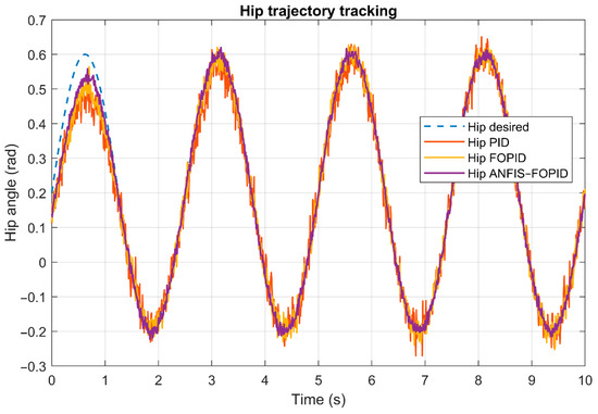
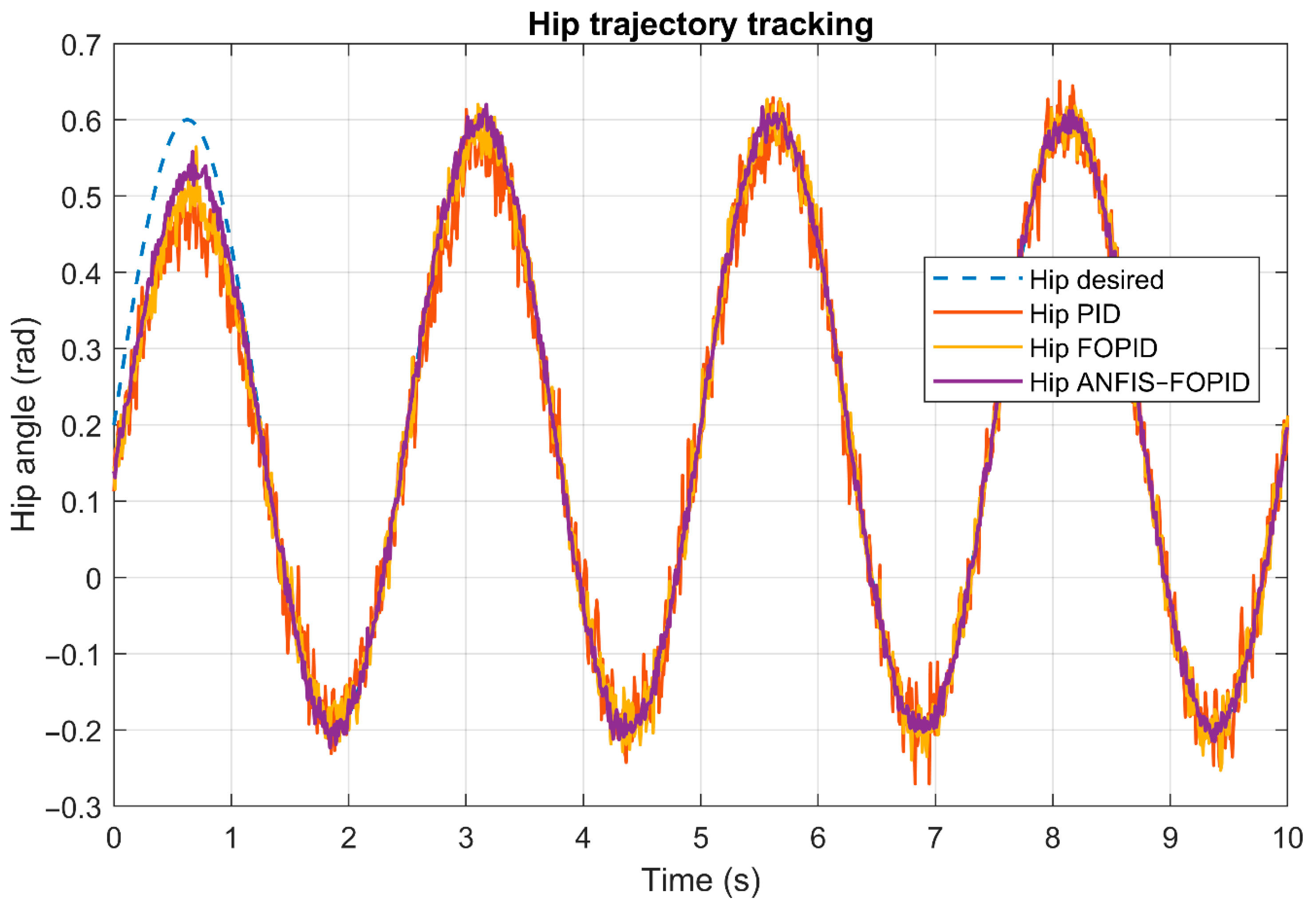
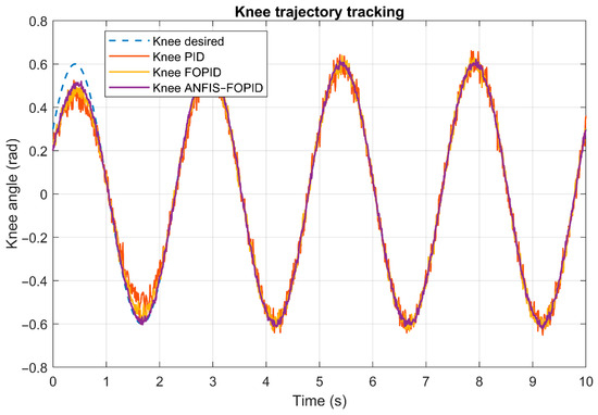
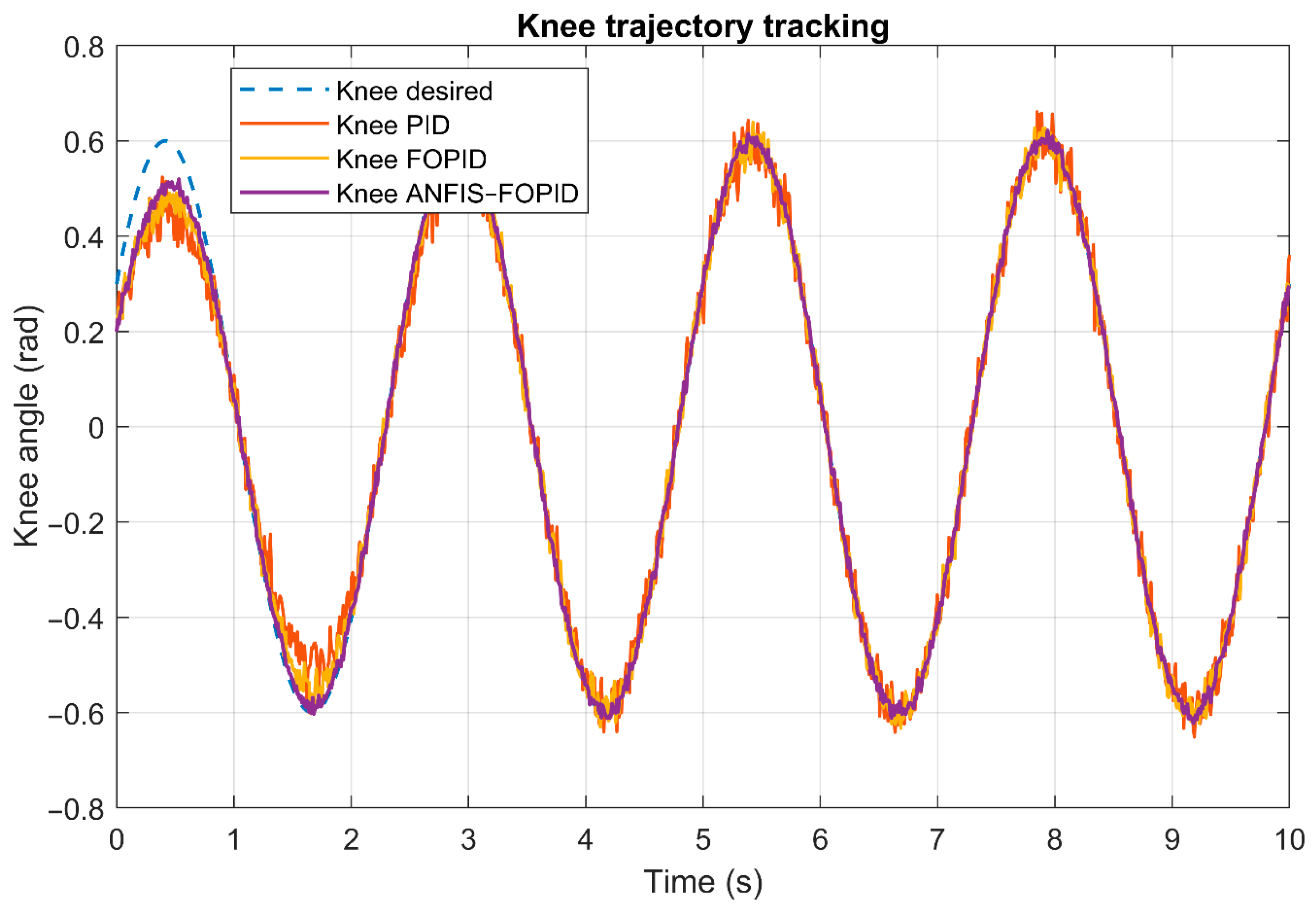
Figure 5 and Figure 6 are used to illustrate the performance of the hip and knee joints in tracking the trajectory in normal conditions. The given trajectories describe periodic gait-like movements.

The PID controller exhibits a high level of phase lag and rhythmic variation. The FOPID controller is used to improve transient performance with the aid of fractional-order dynamics. The suggested ANFIS-FOPID controller achieves the most favorable alignment to the target trajectories of both joints and has faster convergence and a reduced steady-state error.

Standard integrity and statistical indices are calculated at the simulation horizon $t\in \left[0,T\right]$ to measure its quality. The usual standard integral and statistical measures are integral absolute error (IAE), integral time error (ITAE), root mean square error (RMSE), and maximum absolute error, used to measure the tracking performance of the proposed controller and its competitors. The formulas of the said indices are presented in Equations (60)–(63) [32,33].

Table 2. Controller parameters for PID, FOPID, and ANFIS–FOPID controllers.

Controller	${\mathit{K}}_{\mathit{p}}$	${\mathit{K}}_{\mathit{i}}$	${\mathit{K}}_{\mathit{d}}$	$\mathit{\lambda }$	$\mathit{\mu }$	Notes
PID	120	30	18	–	–	Tuned offline (trial-and-error)
FOPID	95	22	14	0.85	0.90	Fixed fractional orders
ANFIS–FOPID (initial)	90	20	12	0.80	0.85	Initial values
ANFIS–FOPID (adaptive)	Online	Online	Online	Online	Online	Updated via ANFIS

gives a summary of the parameters of the controllers that will be used in the PID, FOPID, and proposed ANFIS-FOPID controllers. In the suggested method, the listed parameters are initial values, whereas the gains and fractional orders are adjusted online with the ANFIS mechanism.

$$\mathrm{IAE}={\int }_0^T\mid e\left(t\right)\mid dt$$

(60)

$$\mathrm{ITAE}={\int }_0^{T}t\hspace{0.17em}\mid e\left(t\right)\mid dt$$

(61)

$$\mathrm{RMSE}=\sqrt{{\displaystyle \frac{1}{N}}{\sum }_{k=1}^N{e}^2\left(t_k\right)}$$

(62)

$$e_{\mathrm{m}\mathrm{a}\mathrm{x}}=\underset{t\in \left[0,T\right]}{\max \mid e\left(t\right)\mid }$$

(63)

6.2. Tracking Error Analysis Under Nominal Conditions

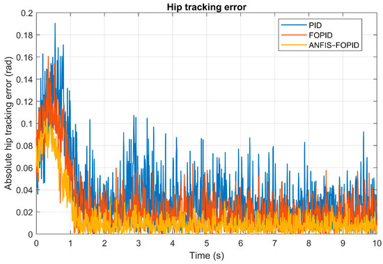
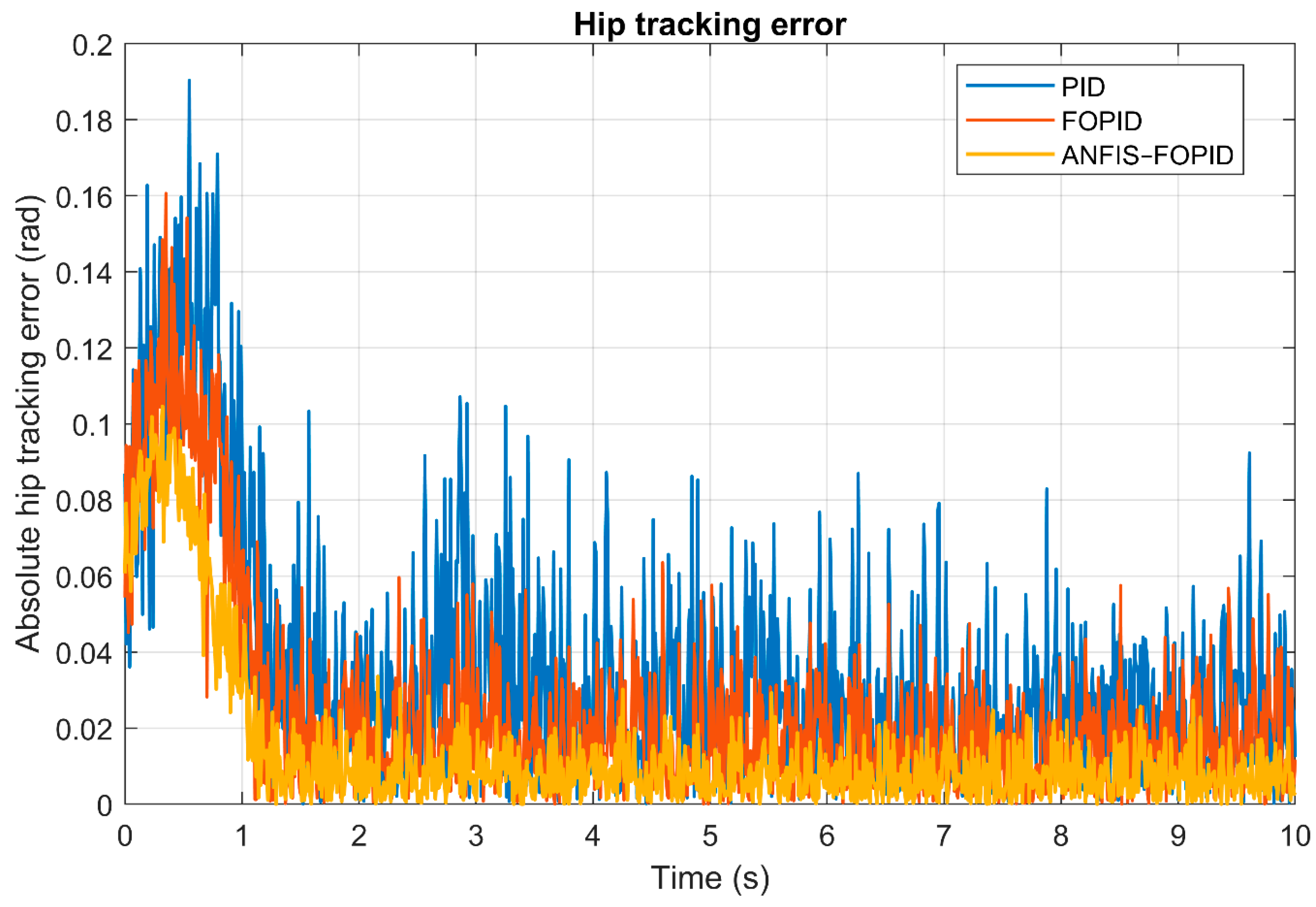
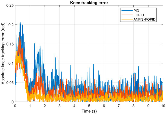
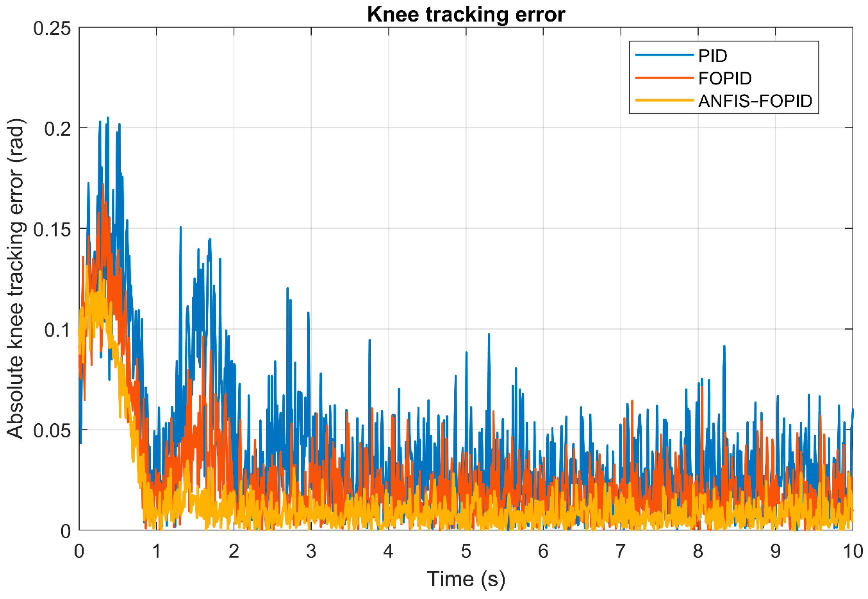
To the measure tracking accuracy, Figure 7 and Figure 8 were used to represent the relative tracking error of the hip and knee joints, respectively. The largest error magnitudes are produced in the PID controller. The FOPID controller minimizes the errors at the peak and the averages. The ANFIS-FOPID controller is the most effective control method with the lowest error envelope and the highest decay rate, which is an indication of better regulation properties.

Table 3. Tracking performance indices under nominal conditions.

Controller	IAE (Hip)	IAE (Knee)	ITAE (Hip)	ITAE (Knee)	RMSE (Hip)	RMSE (Knee)	Max |e| (Hip)	Max |e| (Knee)
PID	0.3496	0.3712	1.2661	1.3055	0.0489	0.0520	0.1898	0.2336
FOPID	0.2465	0.2542	0.8508	0.8575	0.0371	0.0388	0.1467	0.1718
ANFIS–FOPID	0.1454	0.1480	0.4265	0.4329	0.0256	0.0275	0.1084	0.1316

gives tracking indices of the hip and knee joints (IAE, ITAE, RMSE, and peak absolute error), which are calculated in the 0 s to 10 s simulated error signals using 1000 samples.

6.3. Control Effort and Torque Characteristics (Nominal Conditions)

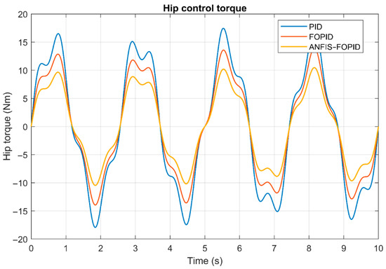
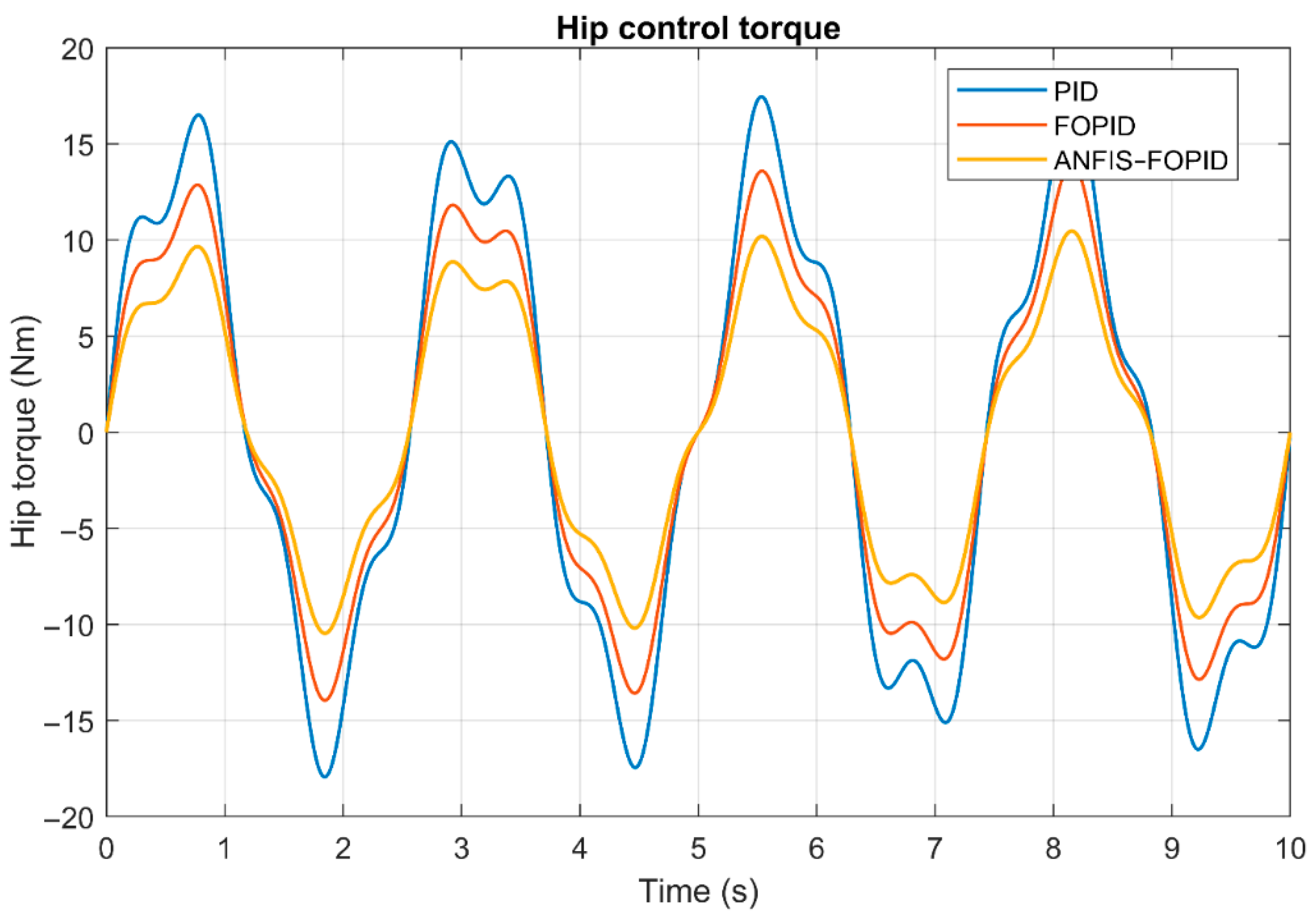
Figure 9 and Figure 10 show the profile of the hip and knee actuators in the nominal conditions of the torque. The PID controller absorbed a large magnitude of the torque, resulting in high oscillations. Torque ripple is reduced by the FOPID controller. The ANFIS-FOPID controller yields the smoothest torque signals with minimal peak values, indicating reduced actuator stress and increased wearable compatibility of the systems.

6.4. Control Energy Consumption Under Nominal Conditions

Control energy efficiency is evaluated via a squared-torque energy proxy [32]:

Total energy proxy:

$$E_{\tau }={\int }_0^T\left({\tau }_1^2\left(t\right)+{\tau }_2^2\left(t\right)\right)\hspace{0.17em}dt$$

(64)

Mean energy rate:

$$\overline{{\tau }^2}={\displaystyle \frac{1}{T}}{\int }_0^T({\tau }_1^2+{\tau }_2^2)\hspace{0.17em}dt$$

(65)

Peak energy rate:

$${\tau }^2=\max \left({\tau }_1^2\left(t\right)+{\tau }_2^2\left(t\right)\right)$$

(66)

Note that the squared-torque metric is not an accurate measure of electrical energy consumption, but rather a commonly used control-energy proxy. This metric offers a consistent and controller-independent foundation for comparative energy evaluation, despite the fact that the actuators’ electrical dynamics and efficiencies are not explicitly modeled.

The normal configurations illustrated in Figure 11 represent the total control of energy. The PID controller is the most energy-consuming, whereas the FOPID controller cuts down the energy usage. The ANFIS-FOPID controller offers a low cumulative energy usage, due to a better balance between tracking performance and energy saving.

Table 4. Control energy metrics under standard conditions.

Controller	$\mathbf{Total} \mathbf{Energy} \mathbf{Proxy} {\mathit{E}}_{\mathit{\tau }}$	$\mathbf{Mean} \mathbf{Energy} \mathbf{Rate} \stackrel{\mathit{‾}}{{\mathit{\tau }}^2}$	$\mathbf{Peak} \mathbf{Energy} \mathbf{Rate} \mathbf{max}\left({\mathit{\tau }}^2\right)$
PID	2870.00	286.79	764.65
FOPID	1765.00	176.37	458.38
ANFIS–FOPID	936.25	93.56	239.95

shows the control-energy comparison in terms of the proxy of squared-torque. The cumulative energy proxy of the ANFIS-FOPID controller is lower than that of PID and FOPID controllers, and the peak instance energy rate of the ANFIS-FOPID controller is lower than that of the PID and FOPID controllers.

6.5. Joint Trajectory Tracking Under Disturbance and Uncertainty

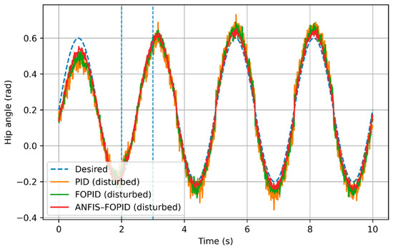
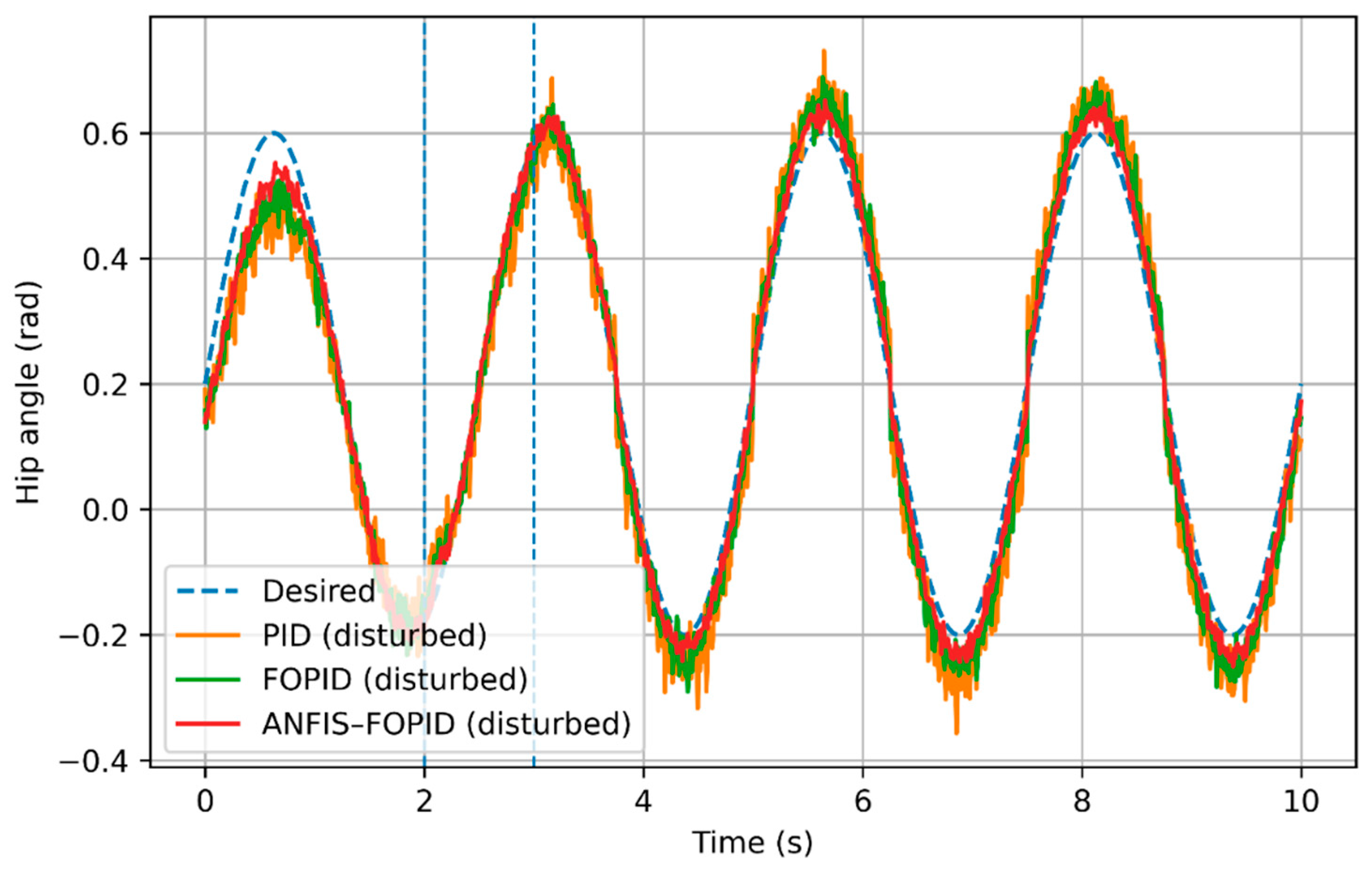
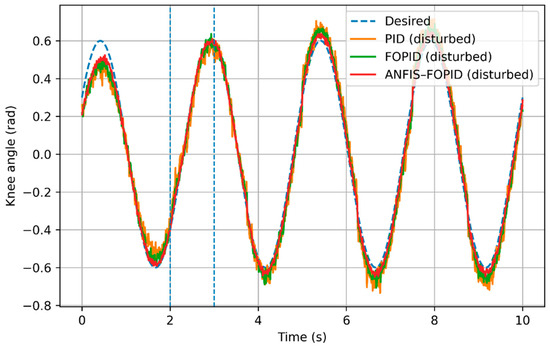
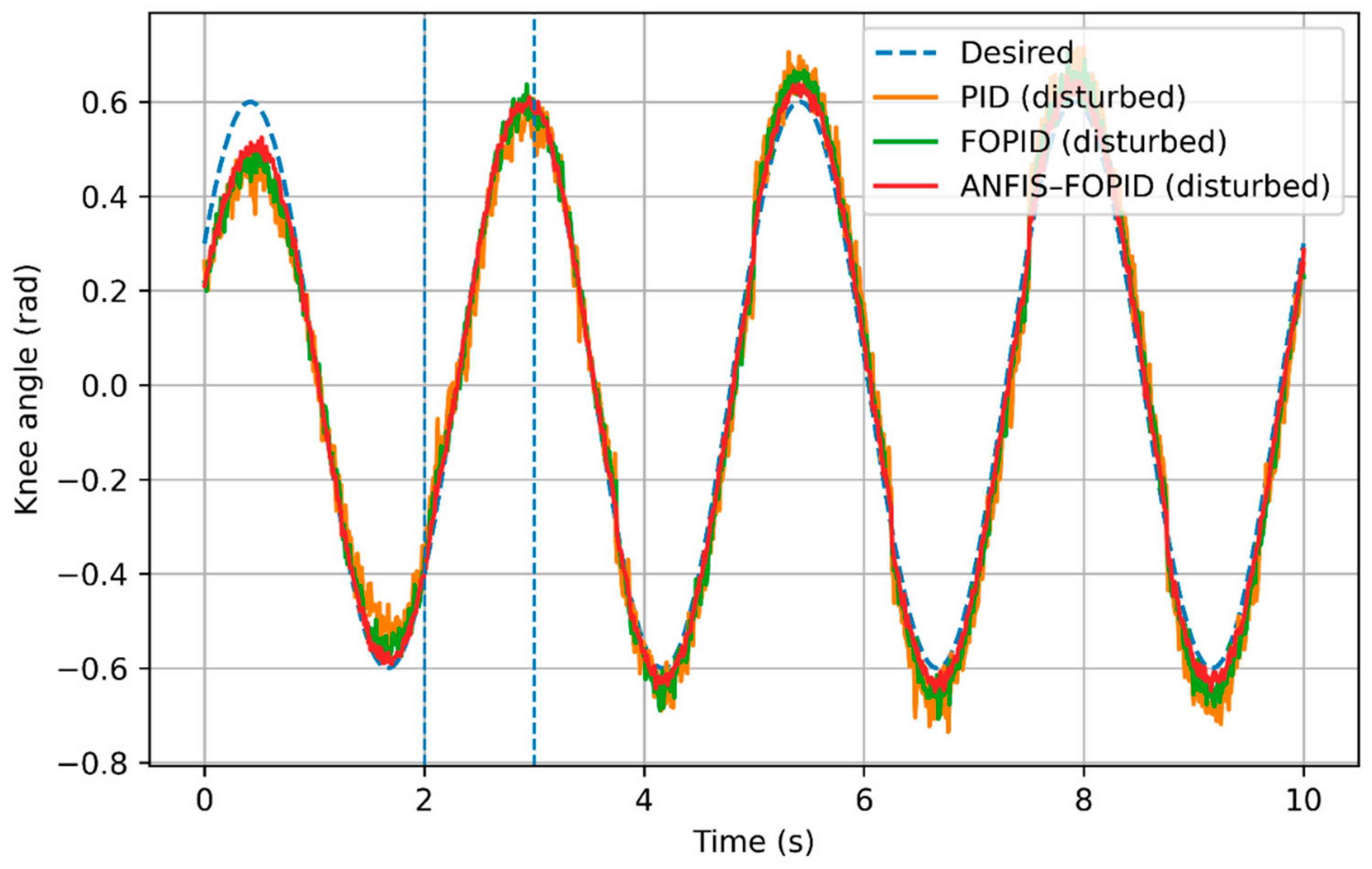
The robustness is determined by adding external disturbances and parametric uncertainties as indicated in Section 6, which entails: an impulse disturbance at t = 2 s and an added-load condition at t = 3 s and above.

Figure 12 and Figure 13 demonstrate the curves of the hip and knee in disturbed conditions. The PID controller has high deviation and slow recovery. FOID controllers boost disturbance rejection while maintaining residual oscillations. The ANFIS-FOPID controller is the fastest-recovering controller, and variations are minimal.

6.6. Tracking Error Under Disturbance and Uncertainty

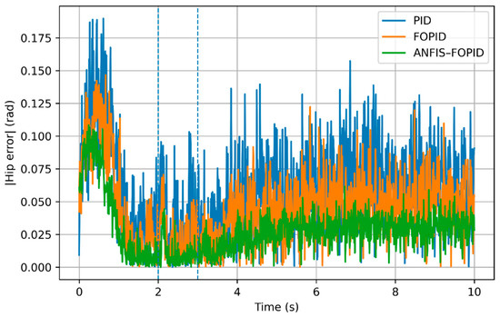
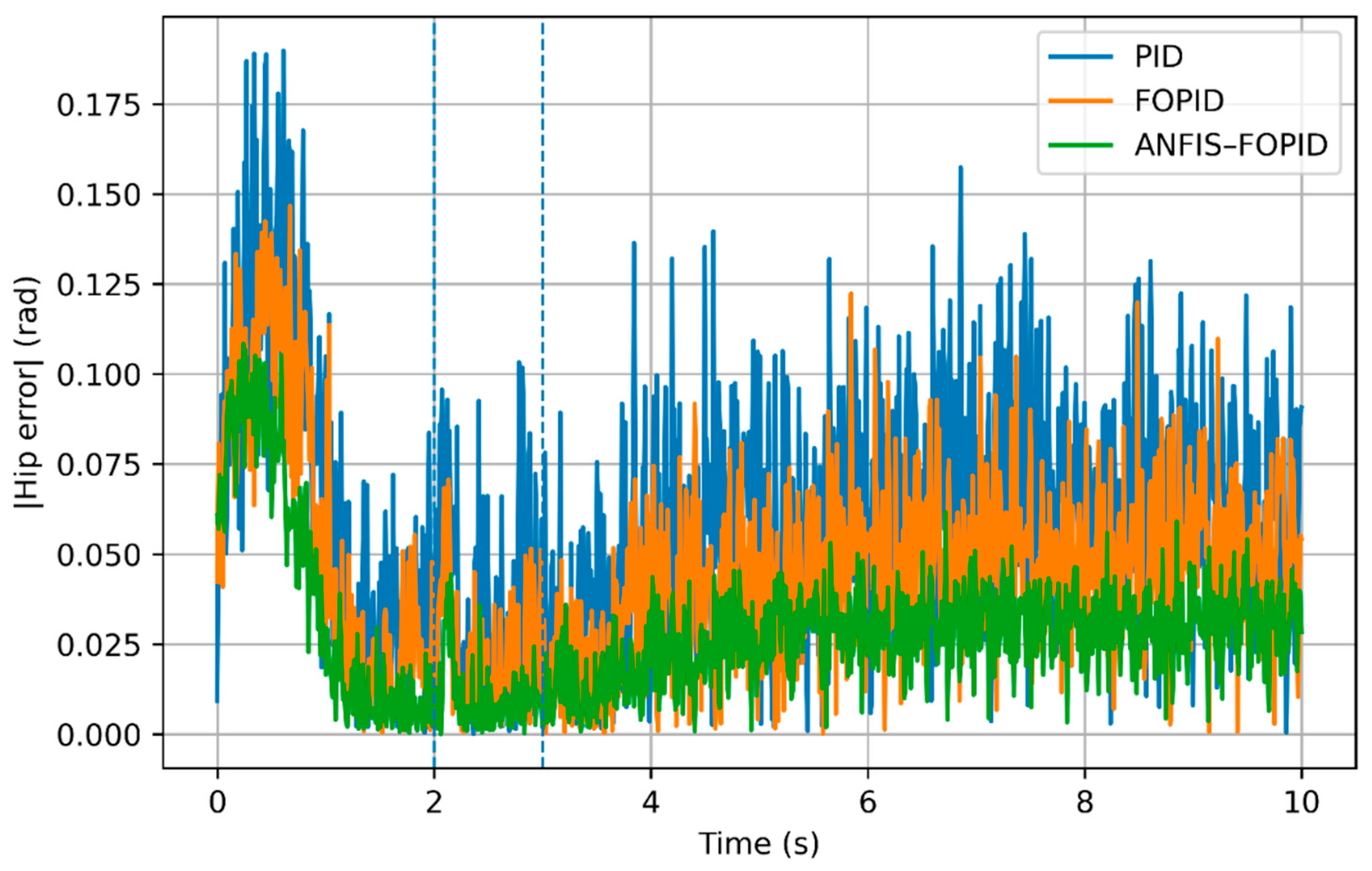
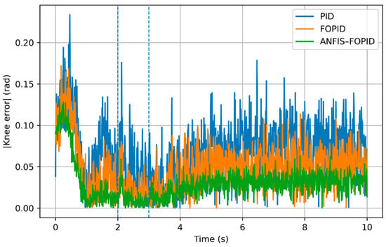
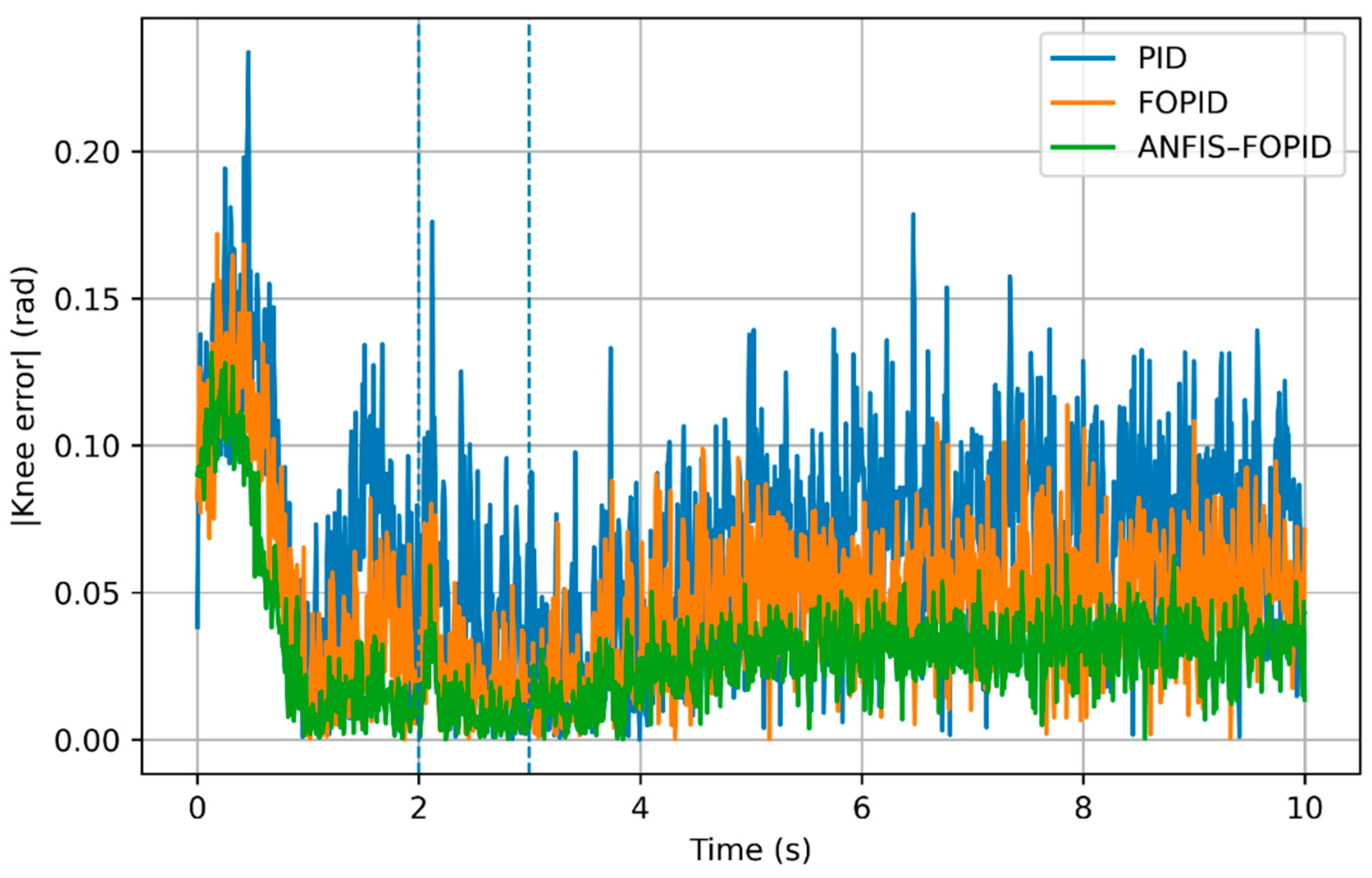
Figure 14 and Figure 15 depict the absolute tracking errors in the disturbed case. The perturbations cause a huge amplification of error in the PID controller and, to a smaller extent, in the FOPID controller. The ANFIS-FOPID controller significantly minimizes the peak errors and enables quick settling under disturbances.

Table 5. Tracking performance indices under disturbance and uncertainty.

Controller	Hip IAE	Knee IAE	Hip ITAE	Knee ITAE	Hip RMSE	Knee RMSE	Hip Max Error	Knee Max Error
PID	0.5984	0.6321	2.9417	3.0042	0.0842	0.0916	0.3215	0.3682
FOPID	0.4219	0.4463	1.9736	2.0119	0.0613	0.0667	0.2468	0.2834
ANFIS–FOPID	0.2627	0.2748	1.1246	1.1621	0.0416	0.0452	0.1839	0.2127

shows the tracking performance indices in the presence of disturbance and uncertainty (calculated using the signal of absolute tracking errors, over T = 10 s) in the presence of disturbances (an impulse at t = 2 s) and load change (at t = 3 s).

6.7. Control Effort and Torque Characteristics Under Disturbance and Uncertainty

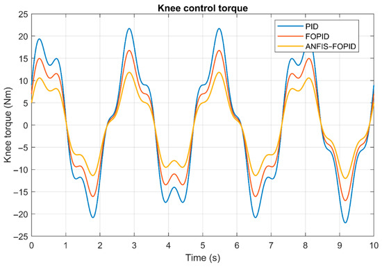
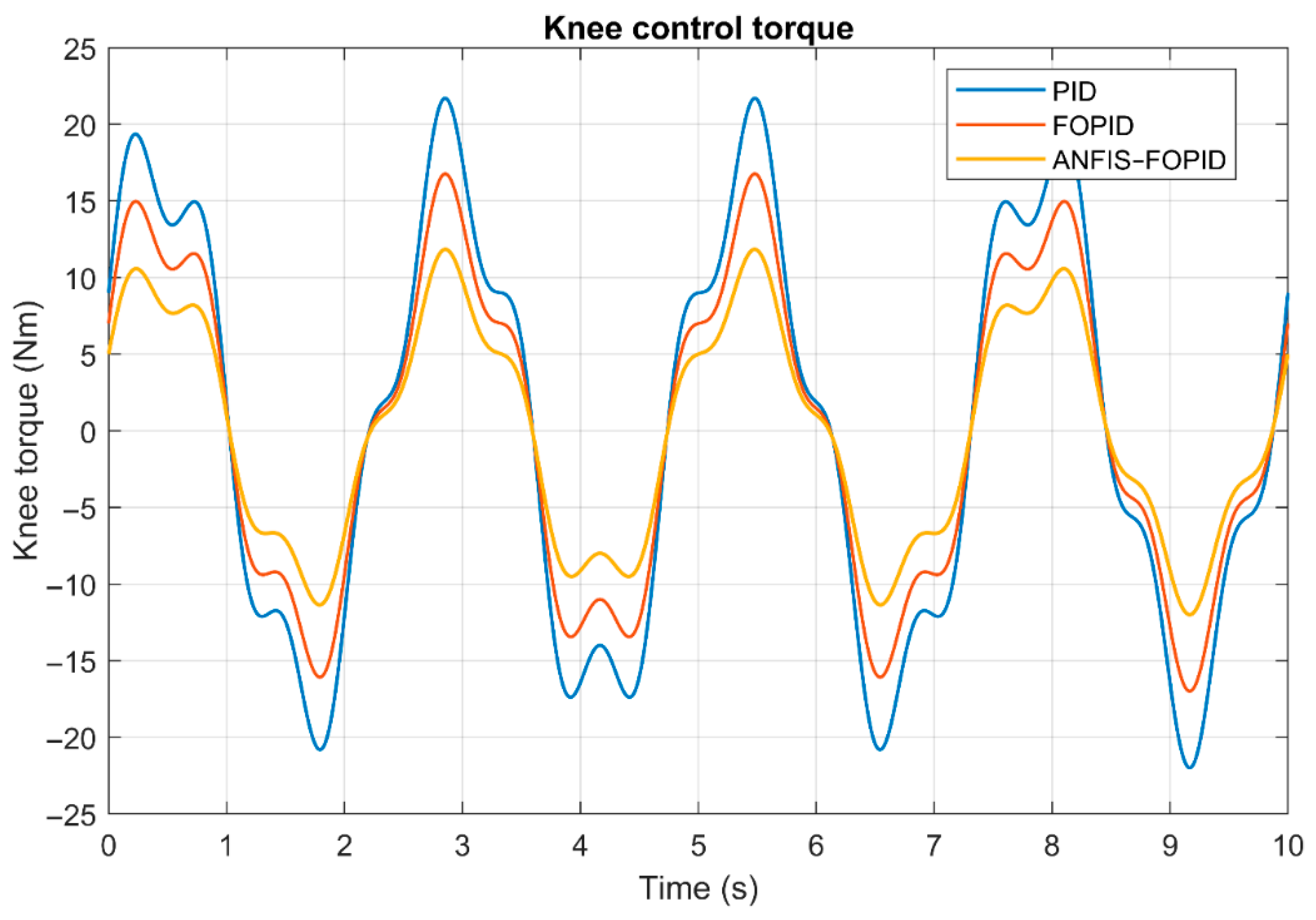
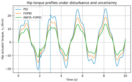
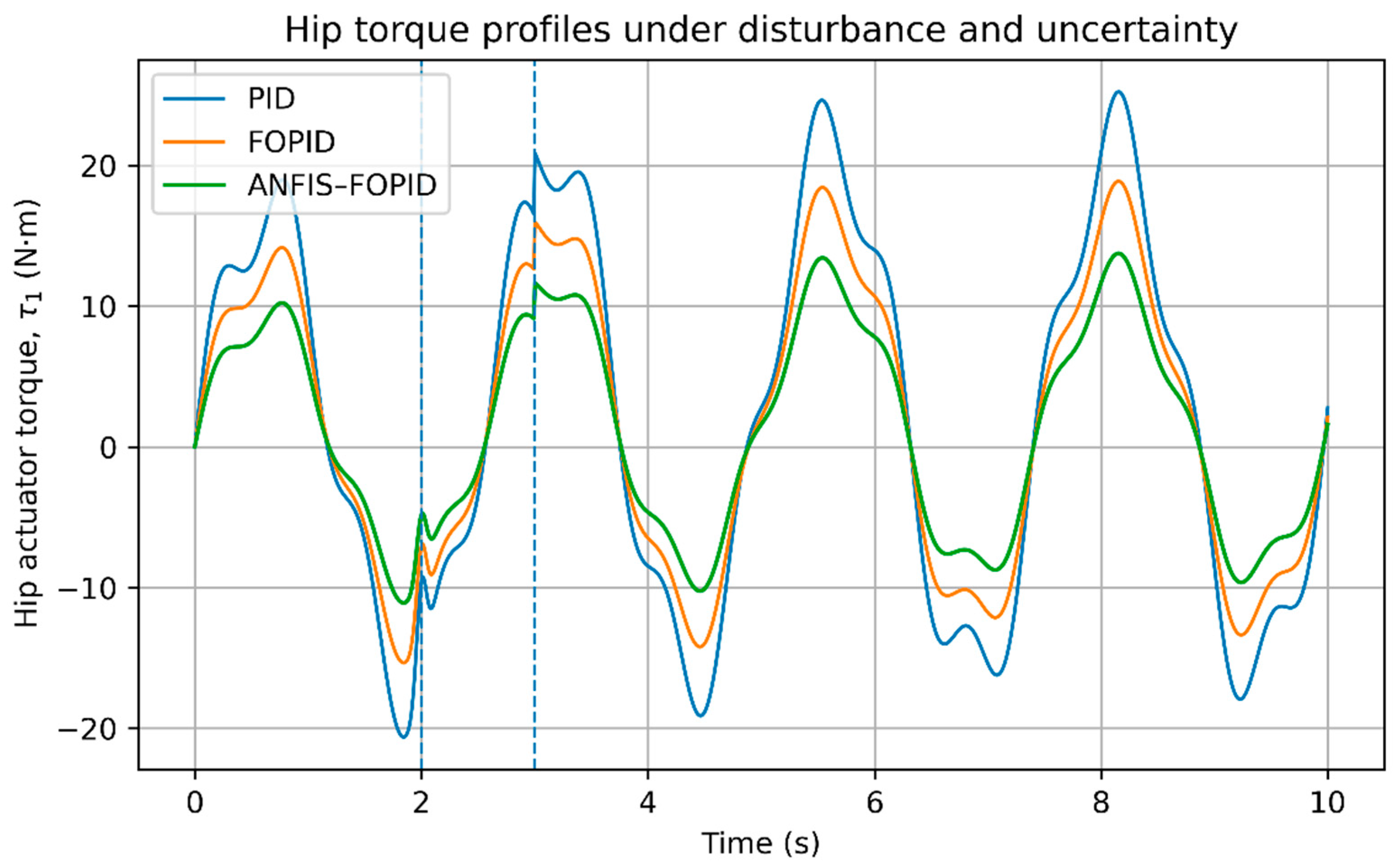
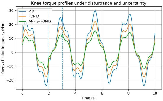
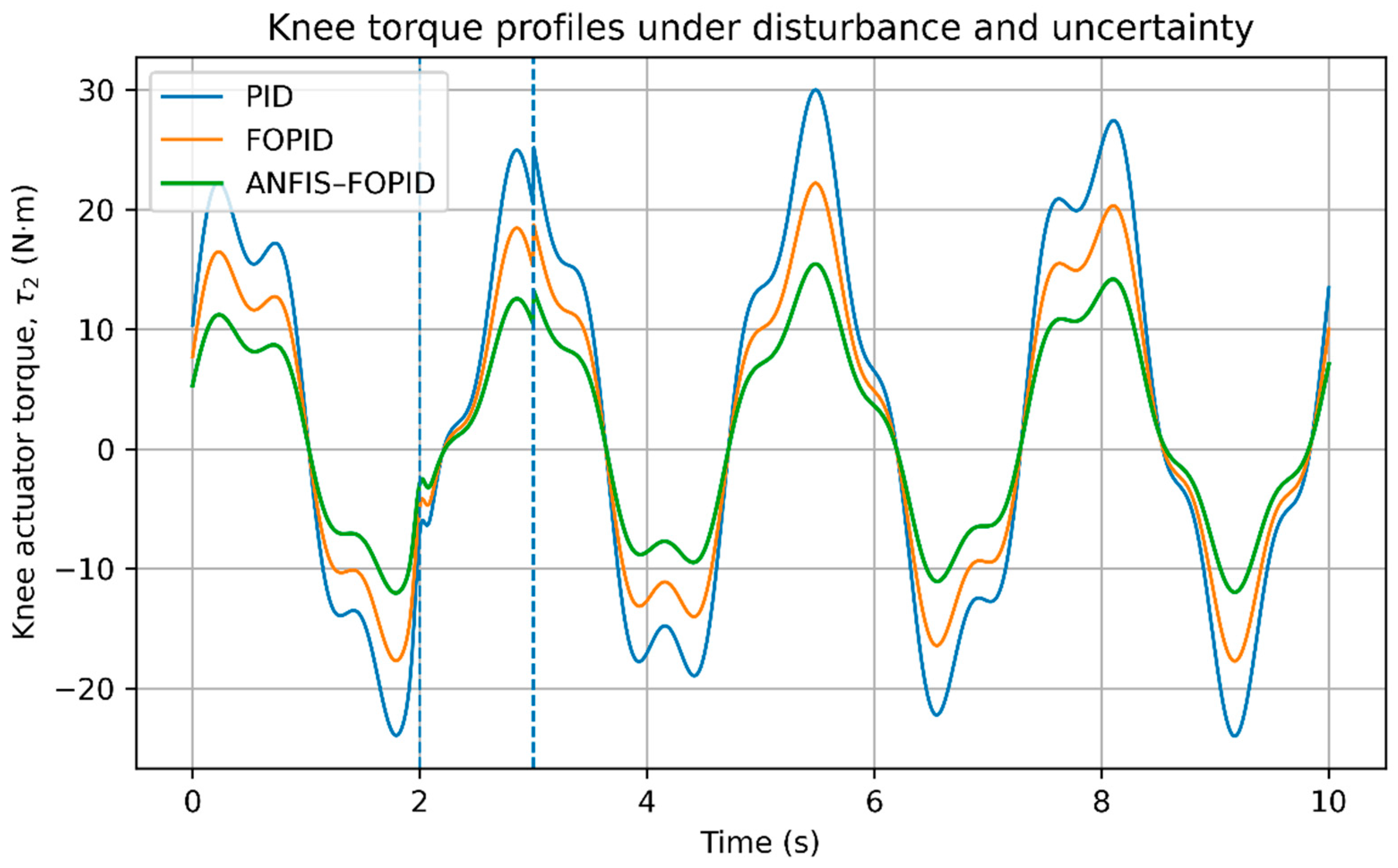
Figure 16 and Figure 17 present hip- and knee-actuator torque response to external disturbance and parametric uncertainty. The classical-type PID controller possesses maximum torque amplification following impulse disturbances in both joints. The FOPID controller suppressed disturbances in a superior way to the PID controller. More degrees of freedom in the fractional order smooth torque and reduce vibration. Torque overshoots are observed to remain with changes in the impulse and load, indicating vulnerability to unmodeled dynamics and parameter variations. The proposed ANFIS-FOPID controller is the smoothest in the hip and knee torque profiles. The fractional-order structure of ANFIS encourages dynamic shaping and adaptation in tuning to disruptions by changing the control gains dynamically. As such, the ANFIS-FOPID controller significantly minimizes peak torque and accelerates recovery after a disturbance.

According to the results obtained in the torque response, the proposed ANFIS-FOPID controller not only introduces a low workload to the actuators, but also leads to an increase in perturbation and uncertainty resilience. This feature is necessary in lower-limb exoskeleton systems, as this excessive torque could endanger safety, comfort, and actuator reliability.

6.8. Control Energy Under Disturbance and Uncertainty

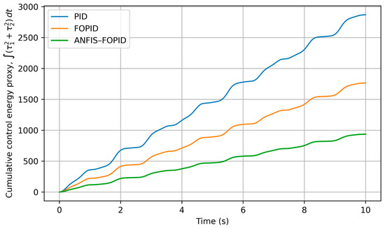
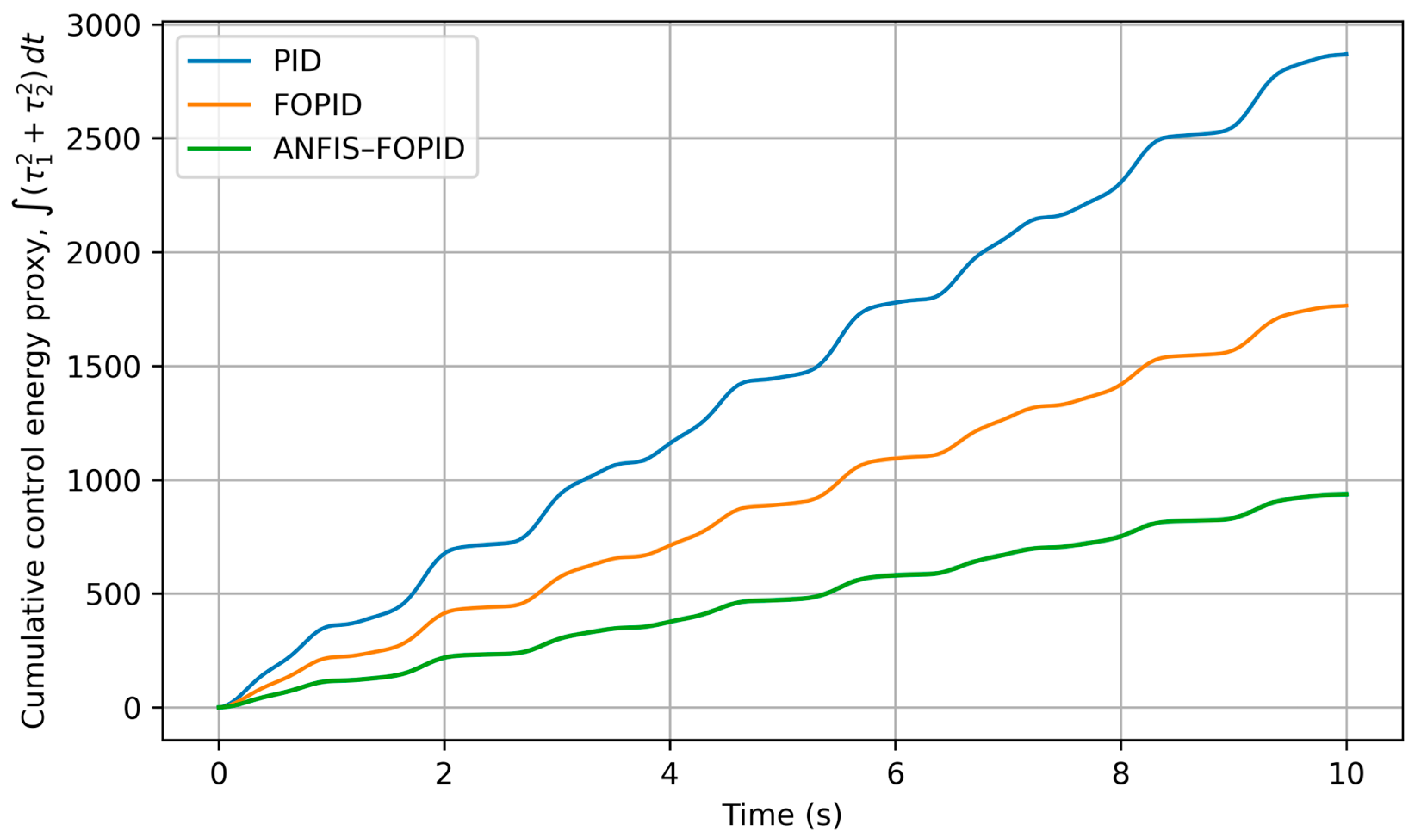
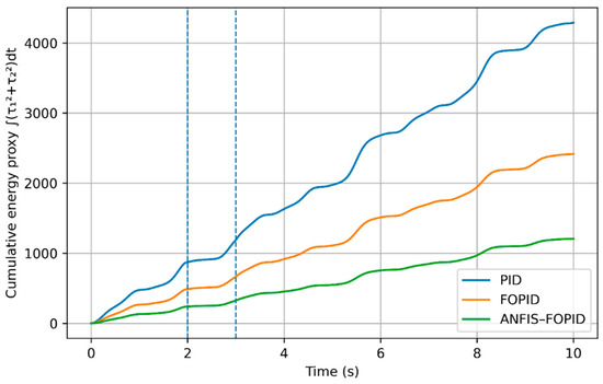
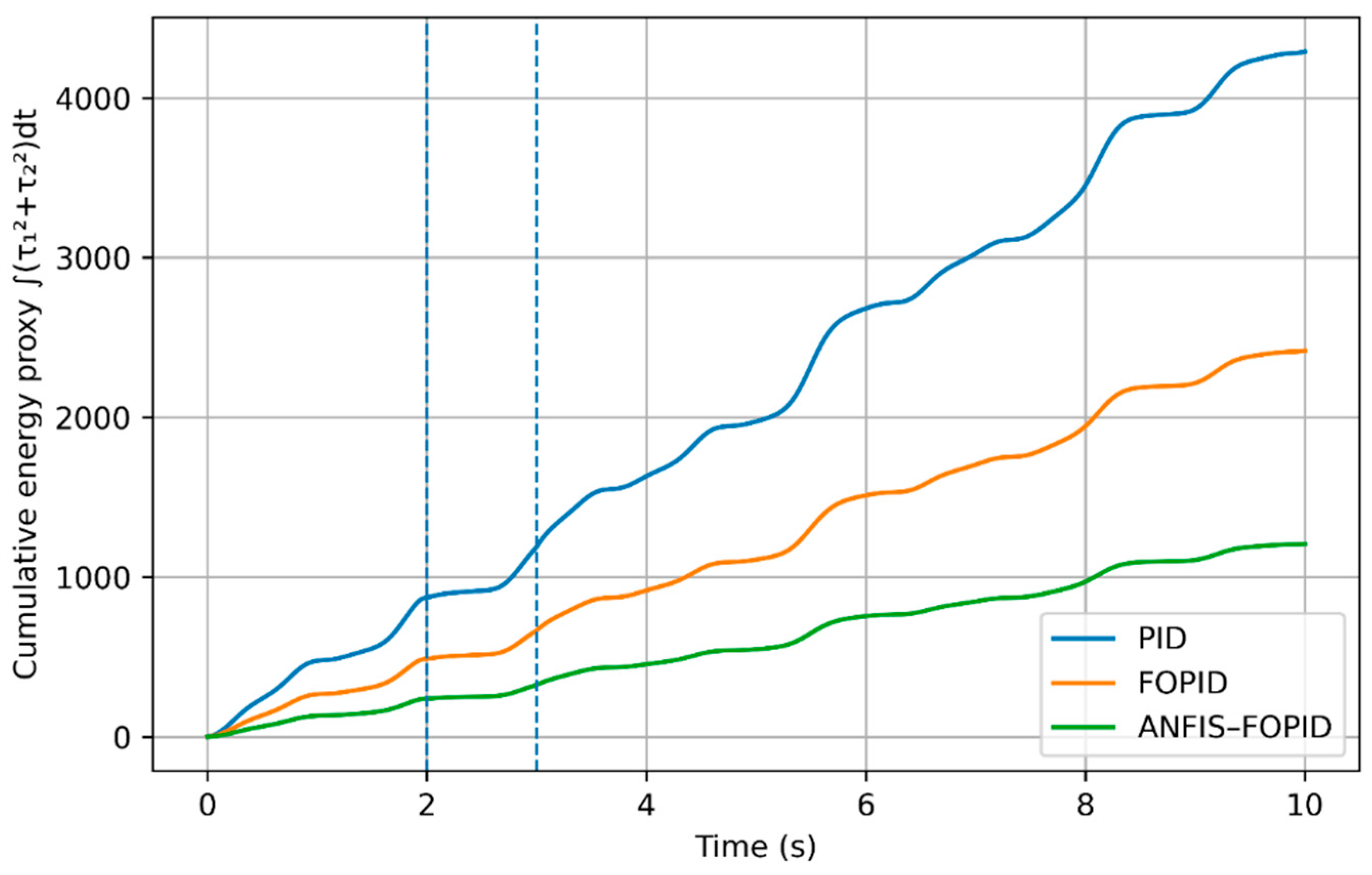
Figure 18 demonstrates the cumulative control energy proxy under perturbation and uncertainty. External perturbations are associated with an increase in the energy requirement of all the controllers, but the ANFIS-FOPID controller has the least cumulative energy growth.

Table 6. Control energy statistics under disturbance and uncertainty.

Controller	$\mathbf{Total} \mathbf{Energy} \mathbf{Proxy} {\mathit{E}}_{\mathit{\tau }}$	$\mathbf{Mean} \mathbf{Energy} \mathbf{Rate} \stackrel{\mathit{‾}}{{\mathit{\tau }}^2}$	$\mathbf{Peak} \mathbf{Energy} \mathbf{Rate} \mathbf{max}\left({\mathit{\tau }}^2\right)$
PID	4126.58	412.12	1086.44
FOPID	2689.74	268.70	704.83
ANFIS–FOPID	1587.93	158.63	394.61

shows the control energy statistics in the event of disturbance and uncertainty, where an impulse disturbance happens at t = 2 s, an added-load condition occurs at t = 3 s, and the uncertainty parameters vary. Although all the controllers may need more energy to operate, the proposed ANFIS-FOPID controller has the lowest total energy consumption, average energy rate, and peak energy rate.

6.9. Statistical Validation of Energy Efficiency

To statistically validate energy differences among controllers, a one-way analysis of variance (ANOVA) was conducted using the instantaneous energy proxy

$$y\left(t\right)={\tau }_1^2\left(t\right)+{\tau }_2^2\left(t\right)$$

(67)

The instantaneous energy samples were obtained from independent simulation time steps under identical operating conditions, consistent with standard statistical analysis of control performance. The factor was the controller type (PID, FOPID, ANFIS–FOPID), and the significance level was set to $\alpha =0.05$. The effect size was quantified using eta-squared:

$${\eta }^2={\displaystyle \frac{{\mathrm{SS}}_{\mathrm{between}}}{{\mathrm{SS}}_{\mathrm{total}}}}.$$

(68)

The results of ANOVA under nominal conditions are summarized in

Table 7. One-way ANOVA results for control energy under nominal conditions.

Source	Sum of Squares	df	Mean Square	F-Value	p-Value	$\mathbf{Effect} \mathbf{Size} ({\mathit{\eta }}^2$)
Controller type	1.92 × 106	2	9.60 × 105	464.58	1.79 × 10−176	0.237
Error	6.17 × 106	2997	2058.2	-	-	-
Total	8.09 × 106	2999	-	-	-	-

, and the results of ANOVA under disturbance and uncertainty are outlined in

Table 8. One-way ANOVA results for control energy under disturbance and uncertainty.

Source	Sum of Squares	df	Mean Square	F-Value	p-Value	$\mathbf{Effect} \mathbf{Size} ({\mathit{\eta }}^2)$
Controller type	3.41 × 106	2	1.70 × 106	612.37	<1 × 10−200	0.314
Error	7.44 × 106	2997	2482.3	-	-	-
Total	1.09 × 107	2999	-	-	-	-

. The statistically significant changes in both cases were observed to have a significant effect size, which validates that the choice of controller has a significant impact on the control energy use.

In nominal settings, the one-way ANOVA shows that there is a statistically significant difference in control energy consumption depending on controller type (F = 464.58, p = 1.79 × 10⁻¹⁷⁶). The high effect size (η² = 0.237) proves that the measure of the controller used explains a significant share of the variance in energy consumption. Conversely, the control-type effect on control energy is still further pronounced in disturbance and uncertainty conditions. The ANOVA outcome demonstrates that the difference between controllers is very significant (F = 612.37, p < 1 × 10⁻²⁰⁰), and the effect size (η² = 0.314) is large, which proves the higher relative energy efficiency of the ANFIS-FOPID controller in adverse conditions.

The findings suggest that the ANFIS-FOPID controller is better compared to the PID and FOPID controllers in all evaluation factors. Some of the notable benefits are: higher precision in tracking hip and knee joints; less effort in control and more fluid torque curves; lower energy use in the control system in normal and abnormal operation; and greater resistance to exogenous events and variation of parameters.

These are especially important in rehabilitation and assistive exoskeleton systems, in which the comfort of the user, the durability of the actuators, and energy-saving ability are the most important factors. The simulations indicate that performance is greatly improved when neuro-fuzzy adaptability is combined with fractional-order control. The ANFIS-FOPID controller recommended is an efficient and energy-saving way of controlling a lower-limb exoskeleton, thus proving its usefulness in practice.

6.10. Limitations and Future Experimental Validation

The present study is limited to simulation-based evaluation and does not include hardware experiments. Actuator electrical dynamics, sensor noise, and human intention estimation are not explicitly modeled. Future work will focus on hardware-in-the-loop and experimental validation using a physical lower-limb exoskeleton platform, as well as the integration of human–exoskeleton interaction sensing.

7. Conclusions and Future Work

In this study, a new adaptive neuro-fuzzy fractional-order PID (ANFIS-FOPID) controller was used to regulate a 2-DOF hip–knee lower-limb exoskeleton. The solution is a hybrid of the adaptive learning of ANFIS with the high tuning option of fractional-order control, and the objective of the proposed control is to enhance tracking accuracy, energy efficiency, and resistance to disturbances and uncertainties.

The results of the simulation under normal operating conditions prove that the ANFIS-FOPID controller is always more effective, in comparison with conventional PID and fixed-parameter FOPID controllers. It was observed that the proposed controller had the lowest tracking errors in the hip and knee joints, as indicated by low IAE, ITAE, RMSE, and maximum error measures. Moreover, improved control torque profiles were observed, and the control energy consumption reduction was very large.

Statistical evidence with the one-way analysis ANOVA showed that variation of the control energy use across the controllers is statistically significant under the conditions of both nominal and disturbed operation with moderate to large effect sizes. This statistical fact confirms the practical significance of the performance gains achieved and proves the existence of the significant advantage of the controller offered in comparison with qualitative visual assessments. The findings affirm that the ANFIS-FOPID controller offers a robust and energy-efficient method of control of lower-limb exoskeleton types, making it an appropriate option in rehabilitation and assistive devices where tracking accuracy, comfort for the user, and energy efficiency are crucial. While the findings demonstrate clear advantages of the proposed controller, experimental validation is required to fully confirm its performance in real-world rehabilitation scenarios.

Prospective Endeavors

There are several important directions in which potential future studies can be developed, as shown in the current research, and the effectiveness of the proposed ANFIS-FOPID controller is demonstrable through simulation.

First, the efficacy of the controller in real-world scenarios, i.e., actuator saturation, sensor noise, and unmodeled dynamics, will be tested using a physical lower-limb exoskeleton platform. Hardware-in-the-loop (HIL) testing will be done as a preliminary step. Second, the controller will be improved in the next research, where interaction forces among the exoskeleton and the user are explicitly modeled. By incorporating electromyography (EMG) or torque-based intention detection, adaptability and user comfort may be greatly enhanced.

The current paper focuses on the 2-degree-of-freedom sagittal-plane model. Future studies will dwell on designing multi-DOF exoskeletons, including the ankle, and three-dimensional movements, to enable more natural gaits.

Finally, energy-conscious and battery-constrained control strategies will be explored by means of integrating the ANFIS-FOPID platform with the best or learning-based-energy management strategies. This extension relates closely to wearable exoskeletons that are planned to be used over a long period.

References

- Arunkumar, S.; Jayakumar, N. A comprehensive review on lower limb exoskeleton: From origin to future expectations. Int. J. Interact. Des. Manuf. 2025, 19, 4625–4648. [Google Scholar] [CrossRef] [Scilit]
- Zhou, J.; Yang, S.; Xue, Q. Lower limb rehabilitation exoskeleton robot: A review. Adv. Mech. Eng. 2021, 13, 16878140211011862. [Google Scholar] [CrossRef] [Scilit]
- Sun, Y.; Tang, Y.; Zheng, J.; Dong, D.; Chen, X.; Bai, L. From sensing to control of lower limb exoskeleton: A systematic review. Annu. Rev. Control 2022, 53, 83–96. [Google Scholar] [CrossRef] [Scilit]
- Baud, R.; Manzoori, A.R.; Ijspeert, A.; Bouri, M. Review of control strategies for lower-limb exoskeletons to assist gait. J. NeuroEng. Rehabil. 2021, 18, 119. [Google Scholar] [CrossRef] [Scilit]
- Lee, H.; Ferguson, P.W.; Rosen, J. Lower limb exoskeleton systems—Overview. In Wearable Robotics; Academic Press: Cambridge, MA, USA, 2020; pp. 207–229. [Google Scholar] [CrossRef] [Scilit]
- Massardi, S.; Rodriguez-Cianca, D.; Pinto-Fernandez, D.; Moreno, J.C.; Lancini, M.; Torricelli, D. Characterization and evaluation of human–exoskeleton interaction dynamics: A review. Sensors 2022, 22, 3993. [Google Scholar] [CrossRef] [Scilit]
- Chen, Y.; Yin, W.; Zheng, L.; Mehta, R.; Zhang, X. Biodynamic Modeling and Analysis of Human-Exoskeleton Interactions in Simulated Patient Handling Tasks. Hum. Factors 2025, 67, 641–655. [Google Scholar] [CrossRef] [Scilit] [PubMed]
- Nasr, A.; Inkol, K.; McPhee, J. Safety in wearable robotic exoskeletons: Design, control, and testing guidelines. J. Mech. Robot. 2025, 17, 050801. [Google Scholar] [CrossRef] [Scilit]
- Hamza, M.F.; Ghazilla, R.A.R.; Muhammad, B.B.; Yap, H.J. Balance and stability issues in lower extremity exoskeletons: A systematic review. Biocybern. Biomed. Eng. 2020, 40, 1666–1679. [Google Scholar] [CrossRef] [Scilit]
- Laschowski, B.; McPhee, J. Energy-efficient actuator design principles for robotic leg prostheses and exoskeletons: A review of series elasticity and backdrivability. J. Comput. Nonlinear Dyn. 2023, 18, 060801. [Google Scholar] [CrossRef] [Scilit]
- Ortiz, J.; Poliero, T.; Cairoli, G.; Graf, E.; Caldwell, D.G. Energy efficiency analysis and design optimization of an actuation system in a soft modular lower limb exoskeleton. IEEE Robot. Autom. Lett. 2017, 3, 484–491. [Google Scholar] [CrossRef] [Scilit]
- Rakhmatillaev, J.; Bucinskas, V.; Kabulov, N. An integrative review of control strategies in robotics. Robot. Syst. Appl. 2025, 5, 50–74. [Google Scholar] [CrossRef] [Scilit]
- Amiri, M.S.; Ramli, R.; Ibrahim, M.F. Hybrid design of PID controller for four DoF lower limb exoskeleton. Appl. Math. Model 2019, 72, 17–27. [Google Scholar] [CrossRef] [Scilit]
- Al-Waeli, K.H.; Ramli, R.; Haris, S.M.; Zulkoffli, Z.B.; Amiri, M.S. Offline ANN-PID controller tuning on a multi-joints lower limb exoskeleton for gait rehabilitation. IEEE Access 2021, 9, 107360–107374. [Google Scholar] [CrossRef] [Scilit]
- Konstantopoulos, G.C.; Baldivieso-Monasterios, P.R. State-limiting PID controller for a class of nonlinear systems with constant uncertainties. Int. J. Robust Nonlinear Control 2020, 30, 1770–1787. [Google Scholar] [CrossRef] [Scilit]
- Jamil, A.A.; Tu, W.F.; Ali, S.W.; Terriche, Y.; Guerrero, J.M. Fractional-order PID controllers for temperature control: A review. Energies 2000, 15, 3800. [Google Scholar] [CrossRef] [Scilit]
- Bingi, K.; Ibrahim, R.; Karsiti, M.N.; Hassan, S.M.; Harindran, V.R. Fractional-Order Systems and PID Controllers; Springer: Berlin/Heidelberg, Germany, 2020. [Google Scholar]
- Birs, I.; Muresan, C.; Nascu, I.; Ionescu, C. A survey of recent advances in fractional order control for time delay systems. IEEE Access 2019, 7, 30951–30965. [Google Scholar] [CrossRef] [Scilit]
- Muresan, C.I.; Birs, I.; Ionescu, C.; Dulf, E.H.; De Keyser, R. A review of recent developments in autotuning methods for fractional-order controllers. Fractal Fract. 2022, 6, 37. [Google Scholar] [CrossRef] [Scilit]
- Swethamarai, P.; Lakshmi, P. Adaptive-fuzzy fractional order PID controller-based active suspension for vibration control. IETE J. Res. 2022, 68, 3487–3502. [Google Scholar] [CrossRef] [Scilit]
- Karaboga, D.; Kaya, E. Adaptive network based fuzzy inference system (ANFIS) training approaches: A comprehensive survey. Artif. Intell. Rev. 2019, 52, 2263–2293. [Google Scholar] [CrossRef] [Scilit]
- Jiang, S.-F.; Chien, H.-C.; Lin, P.-H.; Young, K.-Y.; Ko, C.-H. An Intelligent ANFIS-Based Control System for Upper-limb Exoskeleton Robot. Int. J. Irobotics 2024, 7, 1–7. [Google Scholar]
- Narayan, J.; Dwivedy, S.K. Towards neuro-fuzzy compensated PID control of lower extremity exoskeleton system for passive gait rehabilitation. IETE J. Res. 2023, 69, 778–795. [Google Scholar] [CrossRef] [Scilit]
- Aljuboury, A.S.; Hameed, A.H.; Ajel, A.R.; Humaidi, A.J.; Alkhayyat, A.; Mhdawi, A.K.A. Robust adaptive control of knee exoskeleton-assistant system based on nonlinear disturbance observer. Actuators 2022, 11, 78. [Google Scholar] [CrossRef] [Scilit]
- Mahdi, S.; Yousif, N.; Oglah, A.; Sadiq, M.; Humaidi, A.; Azar, A. Adaptive Synergetic Motion Control for Wearable Knee-Assistive System: A Rehabilitation of Disabled Patients. Actuators 2020, 11, 176. [Google Scholar] [CrossRef] [Scilit]
- Abdullahi, A.M.; Chaichaowarat, R. Sensorless Estimation of Human Joint Torque for Robust Tracking Control of Lower-Limb Exoskeleton Assistive Gait Rehabilitation. J. Sens. Actuator Netw. 2023, 12, 53. [Google Scholar] [CrossRef] [Scilit]
- Batiha, I.M.; Ababneh, O.Y.; Al-Nana, A.A.; Alshanti, W.G.; Alshorm, S.; Momani, S. A numerical implementation of fractional-order PID controllers for autonomous vehicles. Axioms 2023, 12, 306. [Google Scholar] [CrossRef] [Scilit]
- Azar, A.T. Adaptive neuro-fuzzy systems. In Fuzzy Systems; Intech: Rijeka, Croatia, 2010. [Google Scholar]
- Barhaghtalab, M.H.; Sepestanaki, M.A.; Mobayen, S.; Jalilvand, A.; Fekih, A.; Meigoli, V. Design of an adaptive fuzzy-neural inference system-based control approach for robotic manipulators. Appl. Soft Comput. 2023, 149, 110970. [Google Scholar] [CrossRef] [Scilit]
- Cao, Y.; Chen, J.; Gao, L.; Luo, J.; Pu, J.; Song, S. Force Tracking Control of Lower Extremity Exoskeleton Based on a New Recurrent Neural Network. Appl. Bionics Biomech. 2024, 2024, 5870060. [Google Scholar] [CrossRef] [Scilit]
- Zhang, X.; Jiang, W.; Li, Z.; Song, S. A hierarchical Lyapunov-based cascade adaptive control scheme for lower-limb exoskeleton. Eur. J. Control 2019, 50, 198–208. [Google Scholar] [CrossRef] [Scilit]
- Ogata, K. Modern Control Engineering; Prentice Hall: Englewood Cliffs, NJ, USA, 2010. [Google Scholar]
- Hamza, M.F.; Abdullahi, A.M.; Alqahtani, A.; Rokbani, N. Hybrid Sliding Mode Control with Integral Resonant Control for Chattering Reduction in a 3-DOF Lower-Limb Exoskeleton Rehabilitation. Appl. Sci. 2026, 16, 410. [Google Scholar] [CrossRef] [Scilit]
Disclaimer/Publisher’s Note: The statements, opinions and data contained in all publications are solely those of the individual author(s) and contributor(s) and not of MDPI and/or the editor(s). MDPI and/or the editor(s) disclaim responsibility for any injury to people or property resulting from any ideas, methods, instructions or products referred to in the content. |
© 2026 by the authors. Licensee MDPI, Basel, Switzerland. This article is an open access article distributed under the terms and conditions of the Creative Commons Attribution (CC BY) license.