Machine Learning Approaches for Classification of Composite Materials

Abstract

The paper presents a comparative analysis of various machine learning algorithms for the classification of epoxy composites reinforced with basalt fiber and modified with inorganic fillers. The classification is based on key thermophysical characteristics, in particular, the mass fraction of the filler, temperature, and thermal conductivity coefficient. A dataset of 16,056 interpolated samples was used to train and evaluate more than a dozen models. Among the tested algorithms, the MLP neural network model showed the highest accuracy of 99.7% and balanced classification metrics F1-measure and G-Mean. Ensemble methods, including XGBoost, CatBoost, ExtraTrees, and HistGradientBoosting, also showed high classification accuracy. To interpret the results of the MLP model, SHAP analysis was applied, which confirmed the predominant influence of the mass fraction of the filler on decision-making for all classes. The results of the study confirm the high effectiveness of machine learning methods for recognizing filler type in composite materials, as well as the potential of interpretable AI in materials science tasks.

1. Introduction

One of the main areas of materials science is the development and improvement of composite materials. For this purpose, polymer matrices [1,2] modified with inorganic fillers are often used. In particular, the article [3] deals with epoxy composites with different concentrations of cast iron filler and with the analysis of their density, hardness, tensile strength, bending strength, and impact toughness. It was proven that an increase in the cast iron content increases hardness, tensile strength, and impact toughness, but reduces the flexural strength of the material. The main patterns of the influence of the type of binder in glass fiber mats on the properties of epoxy composites with quartz filler were revealed in [4]. The tribological characteristics, hardness, and strength were analyzed, and the different sensitivity of the matrix to the type of binder and the absence of a direct relationship between microhardness and specific wear rate at different quartz contents were shown. Article [5] evaluates the dynamic mechanical properties of polymer composites, taking into account eight parameters, including fiber type, fabric structure, and temperature. Epoxy resins, as organic matrices with excellent mechanical properties and chemical resistance, are discussed in [6]. In particular, it highlights the growing interest in modifying resins with natural “green” fillers from plant waste due to their environmental friendliness, availability, and low cost, which allows for the creation of partially biodegradable and cost-effective composites. The influence of TiO₂/Ti₃C₂ composite particles with micro- and nano-morphology on the tribological and thermomechanical properties of epoxy resin is evaluated in [7]. It was found out that the average density of TiO₂ provided minimal wear. The inclusion of TiO₂/Ti₃C₂ significantly improved the elastic modulus and glass transition temperature of epoxy resin. However, the nonlinear nature of the relationships between the components and process parameters requires further study [8]. Solving such problems should be based on modern data analysis tools. Namely, machine learning, as a key branch of artificial intelligence, is widely used in various fields of human activity, in particular in medicine [9,10,11,12,13,14,15,16], industry [17,18,19,20,21], mechanics [22,23,24,25,26,27,28,29] and materials science [30,31,32,33,34,35,36,37,38,39], finance [40,41,42,43,44,45,46], transportation [47,48,49,50,51,52,53], security [54,55,56,57,58,59], education [60,61,62,63], energy [64,65,66,67,68], and agriculture [69,70,71,72,73]. The application of machine learning methods opens up new opportunities for predicting the performance characteristics of composites based on a limited set of experimental data [31]. In particular, the authors of article [74] analyzed the application of artificial intelligence for predicting the mechanical properties of various types of composites. A well-known deep learning method for predicting the mechanical properties of composite materials is presented in [75,76,77]. The effectiveness of several machine learning algorithms for predicting the tensile strength of polymer matrix composites [78], in particular fiber-reinforced composites [79], was compared. There are known methods for modeling the mechanical characteristics of epoxy composites treated with electric spark hydro-impact [80,81], diagnosing damage to composite materials in aerospace structures [82], and evaluating effective thermal conductivity [83,84]. Similar approaches for composites with hollow glass microspheres are proposed in [85] and developed in [86,87] for predicting the physical and mechanical properties of epoxy composites.

However, the application of machine learning methods for predicting the properties of epoxy composites requires further development.

The aim of this work is to develop and evaluate highly accurate models capable of classifying the type of filler (aerosil, γ-aminopropylaerosil, Al₂O₃, Cr₂O₃) in basalt-reinforced epoxy composites based on their thermophysical and mechanical characteristics, in particular the thermal conductivity coefficient, mass fraction of filler, and temperature, using machine learning methods and apply SHAP analysis to interpret decision-making logic. Further research will focus on calculating computational efficiency for different hardware configurations.

2. Materials and Methods

2.1. Experimental Data and Thermophysical Properties of Epoxy Composites

In his Ph.D thesis, A.G. Mykytyshyn [88] investigated the thermophysical characteristics of filled epoxy composites reinforced with basalt fiber. These results were used as the basis for modeling.

Adding a small amount of chemically active fillers to the epoxy matrix, in particular, 1 part by weight of aerosil and 1 part by weight of γ-aminopropylaerosil per 100 parts by weight of the matrix, significantly increases the thermal conductivity of the material. This is explained by the formation of a strong bond between the polymer matrix and the surface of the filler, which is formed as a result of chemical and chemisorption interactions. However, with a significant increase in the concentration of aerosil, a decrease in thermal conductivity is observed, which is due to an increase in the length of the phase boundary and a weakening of the interaction between the OH groups of the filler and the matrix.

When small amounts of aluminum oxide are added, up to 30 wt.%, the thermal conductivity of the composite remains almost unchanged compared to the unfilled polymer. However, when the Al₂O₃ content exceeds 30 wt.%, its thermal conductivity increases, which is mainly due to the high thermal conductivity of the filler itself. At the same time, there is no specific connection between the filler and matrix phases in such systems.

Composites modified with chromium oxide exhibit the behavior that combines the characteristics of both active (aerosil, γ-aminopropylaerosil) and inactive (Al₂O₃) fillers. The thermal conductivity of such systems is determined by the conflicting influence of several mechanisms. On the one hand, the formation of physical nodes between active centers on the particle surface and the matrix can contribute to increased thermal conductivity at low temperatures due to hydrogen bonds at the phase boundary. On the other hand, as the temperature rises, these bonds are destroyed, which increases thermal resistance and reduces thermal conductivity. At the same time, an increase in filler concentration contributes to an overall increase in thermal conductivity, mainly due to its contribution as a heat-conducting phase.

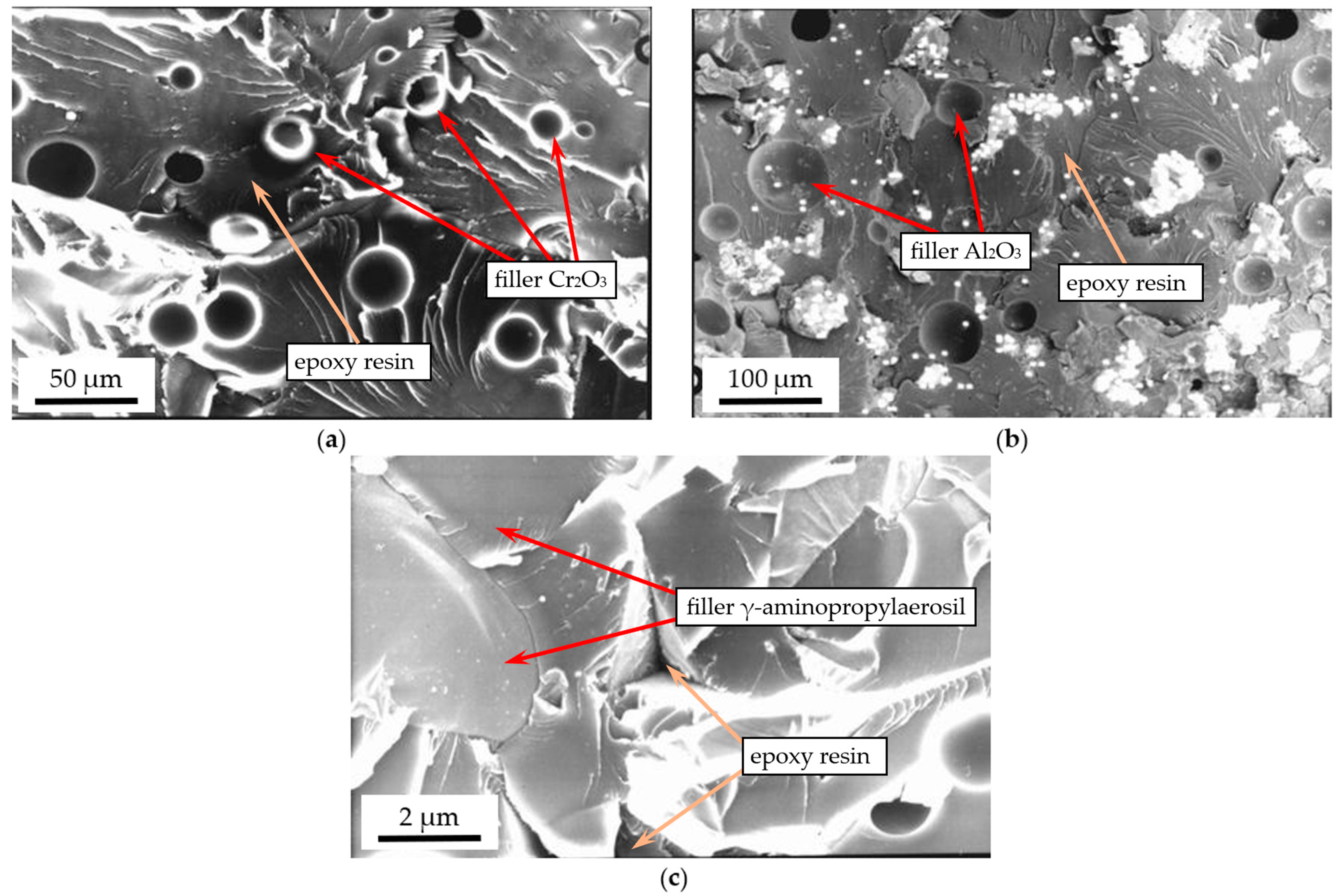
It has been established that the formation of phase structures during the introduction of fillers occurs through the rearrangement of supramolecular structures of the polymer under conditions of thermodynamic incompatibility of components in the process of thermal cross-linking of polymer composite materials. When the composite is cured in the presence of a filler, the kinetics of phase transformations near the surface of the dispersed phase changes significantly, leading to the formation of surface layers in the matrix. The results of studies of the microstructure of PCM containing Al₂O₃ show that the phase boundary between the filler and the polymer matrix is clearly defined. This indicates that there is a kinetic imbalance in the structure of the heterogeneous system in these coatings (Figure 1a). In addition, the uneven distribution of filler per unit area and the presence of micropores significantly impair the thixotropic and cohesive properties of these materials. The phase boundary of the epoxy composite filled with chromium oxide (Figure 1b) is blurred. This indicates the formation of a balanced structure due to the active interaction between the filler and the matrix, which is characterized by a high degree of cross-linking and packing of the binder macromolecules. However, these coatings contain minor microcracks, which characterizes the stress state of the system due to insufficient diffusion processes. Micrographs of the fracture of polymer composites containing γ-aminopropyl aerosil (Figure 1c) clearly show elements of loosening of the material structure, which leads to the formation of a thermodynamically balanced and kinetically stable structure of the surface layers of PCM. Obviously, when this filler is introduced, a significant increase in the viscosity of the material is observed, which provides a wide range of temperature gradients during thermal polymerization, and at the same time, a polymer composite system with high internal stress indicators is formed.

The thermophysical characteristics of filled epoxy composites reinforced with basalt fiber are presented in

Table 1. Composition of the filled epoxy polymers reinforced with basalt fiber [88].

Filler	Concentration, wt %	Thermal Coefficient of Linear Expansion, a × 10–5, K–1
		298K	323K	348K	373K	398K
Aerosil	2	0.52	0.49	0.45	0.46	0.51
	6	0.36	0.34	0.32	0.34	0.33
	12	0.31	0.25	0.29	0.28	0.31
γ-aminopropy- laerosil	2	0.56	0.52	0.50	0.52	0.53
	6	0.44	0.41	0.38	0.42	0.44
	12	0.34	0.28	0.26	0.31	0.32
Cr2O3	30	0.35	0.31	0.29	0.29	0.33
	50	0.48	0.43	0.40	0.41	0.42
	100	0.72	0.69	0.65	0.64	0.63
Al2O3	30	0.40	0.40	0.40	0.41	0.38
	50	0.54	0.53	0.50	0.51	0.54
	100	0.66	0.63	0.60	0.61	0.63

.

The thermophysical characteristics of polymer composite materials are determined by the nature and concentration of the filler, as well as the cross-sectional area of its surface. These properties can be improved by introducing fillers that are chemically active with respect to the matrix and capable of forming strong interfacial bonds with the polymer. Such bonds are formed as a result of chemical and chemisorption interactions between the macromolecules of the binder and the surface of the filler particles, which ensures more efficient heat transfer in the composite.

2.2. Dataset and Correlation Analysis

The data presented in Table 1 [88] was used to form a dataset and create machine learning models for classifying fillers. The composite thermal conductivity coefficient (TCC), filler concentration, its mass fraction of the filler concentration (MFFC), and temperature (T) were selected as input variables, while the output variable was the type of epoxy composite: aerosil (class 1), γ-aminopropylaerosil (class 2), aluminum oxide (class 3), and chromium oxide (class 4).

The experimental data was interpolated to form an expanded dataset of 16,056 elements, which ensured better model training quality. Data interpolation was performed separately for each filler class, which prevented cross-influence between them. The data were interpolated using two-dimensional B-splines (RectBivariateSpline) on a rectangular grid for the variables of mass fraction of the filler concentration and temperature with parameters kx = 2, ky = 3, s = 0, which corresponds to accurate interpolation without smoothing. The dependent variable was selected as the composite thermal conductivity coefficient, which was considered as a continuous function of MFFC and T. New points were formed exclusively within the initial ranges of each class without the use of extrapolation, which ensured the preservation of the characteristic thermophysical relationships inherent in the corresponding filler.

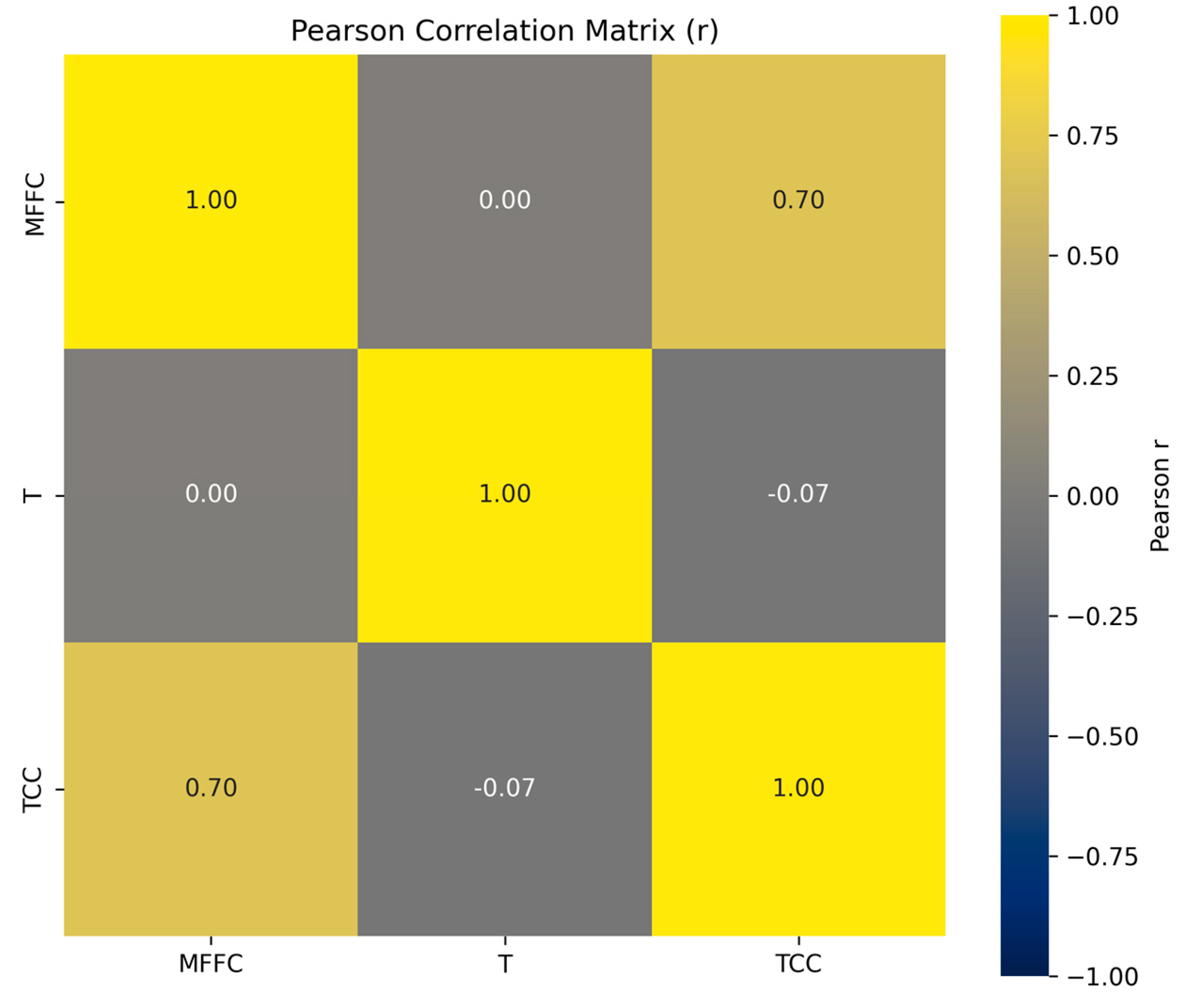
Figure 2 shows a heat map of the Pearson correlation coefficients between three input variables (MFFC, T, and TCC).

The Pearson correlation coefficient between TCC and MFFC was found to be 0.696 (95% CI [0.54; 0.81], p < 0.001), which statistically confirms a strong and significant direct linear relationship between the thermal conductivity coefficient and the mass fraction of the filler. An increase in the amount of filler in the composite significantly increases its thermal conductivity. This is physically correct, since most fillers have higher thermal conductivity than the matrix. This finding is further supported by non-parametric tests (Spearman’s ρ = 0.35, p < 0.01; Kendall’s τ = 0.24, p < 0.05), indicating the robustness of the observed association. The correlation between MFFC and T is 0, indicating no linear relationship between the mass fraction of the filler and the temperature. This indicates that temperature has no effect on the distribution or concentration of the filler in this experiment. A small negative correlation value of −0.07 indicates a very weak negative relationship between temperature and thermal conductivity. However, such a low value allows us to consider these variables to be almost independent in terms of linear relationships. Therefore, the most significant factor determining the thermal conductivity coefficient of the composite is the filler concentration. Temperature does not affect either thermal conductivity or filler concentration within the analyzed data.

During training, the dataset was divided into two unequal parts: training and test samples. For the training sample, 70% of the data was randomly selected, while 30% was left for evaluating the quality of the predictions. This division (70/30) provided enough data for effective training of pattern detection models and also allowed for a reliable assessment of prediction accuracy.

2.3. Machine Learning Algorithms for Classification Tasks

The following main categories have been identified: linear classifiers (Logistic Regression, Stochastic Gradient Descent Classifier and Ridge Classifier), ensemble methods (Extremely Randomized Trees Classifier, Categorical Boosting Classifier, eXtreme Gradient Boosting Classifier, and Histogram-based Gradient Boosting Classifier), Bayesian classifiers (Gaussian Naïve Bayes and Multinomial Naïve Bayes), Support Vector Machines and k-Nearest Neighbors, as well as neural networks such as Multi-Layer Perceptron.

2.3.1. Naive Bayes Classifiers

Gaussian Naive Bayes (GaussianNB) is a simple Bayesian classifier that models the values of features for each class using a normal (Gaussian) distribution. During training, it is used to estimate the mean and variance of each feature within a class, and during prediction, Bayes’ rule is applied, combining these probabilities with the a priori probability of the class [89,90,91]. The algorithm learns to predict very quickly and handles a large number of features well. However, its assumptions about feature independence and normal distribution are not always true, which sometimes reduces the accuracy of classification.

Multinomial Naïve Bayes (MultinomialNB) is a variant of the naïve Bayes classifier that assumes that the features within each class are multinomially distributed [92,93]. During training, the algorithm estimates the conditional probabilities of features in each class, then calculates the probabilities for a new sample and selects the class with the highest probability. The algorithm is fast and resource-efficient.

2.3.2. Linear Classifiers

Logistic Regression is a linear classification method that estimates the probability of an object belonging to a certain class using a logistic function. The model is trained by maximizing likelihood, which is equivalent to minimizing logistic loss with L2 regularization by default [94,95].

Stochastic Gradient Descent Classifier (SGDClassifier) is a classifier that trains a linear model using stochastic gradient descent, an iterative optimization method that updates the model weights after processing each individual sample. It can apply L1 or L2 regularization. This ensures high training speed and model scalability, which is especially important for large datasets [96,97].

Ridge Classifier is a linear classifier that minimizes quadratic loss (as in linear regression) but adds L2 regularization (Ridge), then converts continuous outputs to class predictions. This approach is often faster than logistic regression and more robust to multicollinearity [98,99].

2.3.3. Support Vector Machines and k-Nearest Neighbors

Support Vector Machine (SVM) is a machine learning method that determines the optimal line or hyperplane in classification tasks that separates classes in such a way that the distance to the nearest points of each class is maximized. These nearest points are called support vectors, and they determine the location of the boundary. If the data is not linearly separable, it is first transformed into a higher-dimensional space using a kernel, most often RBF, polynomial, or sigmoidal. The ability of the model to avoid both underfitting and overfitting depends on the choice of kernel and its parameters, as well as on the penalty coefficient [100,101].

k-Nearest Neighbors (kNN) is a simple classification algorithm that does not require training. To determine the class of a new object, it finds the k nearest samples from the training set using a given distance metric, such as Euclidean, and selects the class that occurs most frequently among these neighbors [102,103]. The method is sensitive to the scale of features, so the data should be normalized before using it. The algorithm is easy to implement and intuitive, but with large amounts of data, it can be slow at the prediction stage.

2.3.4. Ensemble Methods

Extreme Gradient Boosting Classifier (XGBClassifier) is a classification tool that implements the gradient boosting method with extensions to improve speed and quality. It builds a sequence of decision trees, where each new tree attempts to correct the errors of the previous ones. The algorithm supports regularization, which reduces the risk of overfitting, automatically handles missing values, allows early stopping, parallel training, and scales well to large datasets [104,105].

Categorical Boosting Classifier (CatBoostClassifier) is a classification algorithm that implements gradient boosting with a focus on the effective processing of categorical features. Unlike most other algorithms, it does not require the prior conversion of such features into numerical values, as it has built-in mechanisms for encoding them. CatBoostClassifier creates a sequence of trees, each of which refines the errors of the previous ones, and uses special techniques to reduce bias and overfitting [106]. The algorithm provides high accuracy, works consistently with tabular data, and is easy to use.

Extremely Randomized Trees Classifier (ExtraTreesClassifier) is an ensemble classification method based on building a large number of random decision trees. Unlike Random Forest, where optimal splits in each node are sought according to a specific criterion, ExtraTrees selects split thresholds randomly, which increases model stability and speeds up training. Each tree is trained on the entire dataset (without bootstrapping) or on a subset of it, and the final decision is made by a majority vote of the trees. This approach is well-scaled and noise-resistant [107,108].

Histogram-based Gradient Boosting Classifier (HistGradientBoostingClassifier) is a classifier that implements gradient boosting of decision trees based on histogram discretization of features. Instead of exact feature values, the algorithm uses values that have been pre-divided into binary intervals (histograms), which significantly speeds up tree construction and reduces memory consumption. This approach is particularly effective for large and high-dimensional datasets. In addition, the model supports regularization, early stopping, and handling of missing values [109].

2.3.5. Neural Networks Type Multi-Layer Perceptron

Multi-Layer Perceptron (MLP) is a type of artificial neural network that contains several sequentially connected layers of neurons (input layer, one or more hidden layers, and output layer). Each neuron in a layer is connected to all neurons in the next layer, and signals are transmitted through nonlinear activation functions, allowing the model to find complex nonlinear dependencies. The network is trained using the backpropagation method, applying gradient descent. MLP is used for both classification and regression, and is the basic form of a feedforward neural network [110].

2.4. Performance Metrics for Classification Models

The performance indicators of classification models, including Accuracy, Recall, Specificity, Precision, F-score, and G-Mean, were calculated based on standard formulas using the values of basic metrics:

• True Positive (TP) is the number of cases where the filler class is predicted correctly, i.e., the model correctly classified the sample as belonging to the corresponding class;
• True Negative (TN) is the number of cases where the model correctly determined that the sample does not belong to a particular filler class;
• False Positive (FP) is the number of cases where the model incorrectly classified the sample as belonging to the filler class, although in reality it did not belong to it;
• False Negative (FN) is the number of cases where the sample belonged to a certain filler class, but the model incorrectly classified it as belonging to another class.

A confusion matrix was constructed for each machine learning algorithm, reflecting the distribution of predicted and actual classes. Analysis of this matrix allowed for a detailed assessment of which classes were predicted incorrectly.

These four basic categories of classification results made it possible to obtain a number of derivative metrics that are widely used for the quantitative assessment of the accuracy, generalization ability, and reliability of models in multi-class classification tasks.

Accuracy is the proportion of all correctly classified objects among the total number:

$$Accuracy={\displaystyle \frac{TP+TN}{TP+TN+FP+FN}},$$

(1)

Precision shows what proportion of predicted positive classes the model classified correctly:

$$Precision={\displaystyle \frac{TP}{TP+FP}},$$

(2)

Recall evaluates the ability of a model to detect all objects of a certain class:

$$Recall={\displaystyle \frac{TP}{TP+FN}},$$

(3)

Specificity reflects the model’s ability to avoid false positive classifications:

$$Specificity={\displaystyle \frac{TN}{TN+FP}},$$

(4)

F1-Score is the harmonic mean between Precision and Recall and is used in cases where a balance between Precision and Recall is required. In particular, a high F1-Score indicates a well-balanced model:

$$F1-Score={\displaystyle \frac{2·Recall·Precision}{Recall+Precision}},$$

(5)

G-Mean is the geometric mean of Recall and Specificity, which allows us to evaluate the balance of the model for both positive and negative classes. In particular, the closer G-Mean is to 1, the better the model works for both positive and negative cases:

$$G-Mean=\sqrt{Recall·Specificity}$$

(6)

All of the above metrics were calculated for each machine learning algorithm, and a comprehensive comparison of their effectiveness was carried out.

3. Results and Discussion

For each machine learning method, error matrices and histograms of model confidence levels were constructed, and the main classification metrics were calculated. Since neural networks showed the highest accuracy among all the algorithms studied, an extended analysis was performed for the MLP model. In particular, Precision–Recall and ROC curves, as well as learning dynamics plots, were additionally presented. In addition, SHapley Additive exPlanations (SHAP) analysis was employed to interpret model decisions, evaluate the probability distribution of predictions, and analyze the impact of input features on the results. This approach contributed to a deeper understanding of the mechanisms of the neural network.

3.1. Results of Naive Bayes Classifiers

In the GaussianNB model that was created based on hyperparameter optimization using GridSearchCV, the best value for the variation smoothing parameter is var_smoothing = 1 × 10⁻⁹. This ensured numerical stability during the estimation of feature variances. The a priori probabilities of classes were not specified but were determined automatically from the training data. After parameter selection, the model was additionally wrapped in a probability calibrator using the CalibratedClassifierCV method with the prefit mode and sigmoid calibration. This ensured reliable probabilistic estimates of predictions.

In the MultinomialNB model, built using GridSearchCV, the best parameter was alpha = 0.001, which corresponds to the lowest level of Laplace smoothing among the studied options. This automatic selection indicates a minimal need for probability regularization. We also used a priori class probabilities, which were determined automatically. After tuning, the classifier was wrapped in the CalibratedClassifierCV calibrator in prefit mode with a sigmoid function. The result is an accurate and interpretable model suitable for probabilistic analysis of classification results.

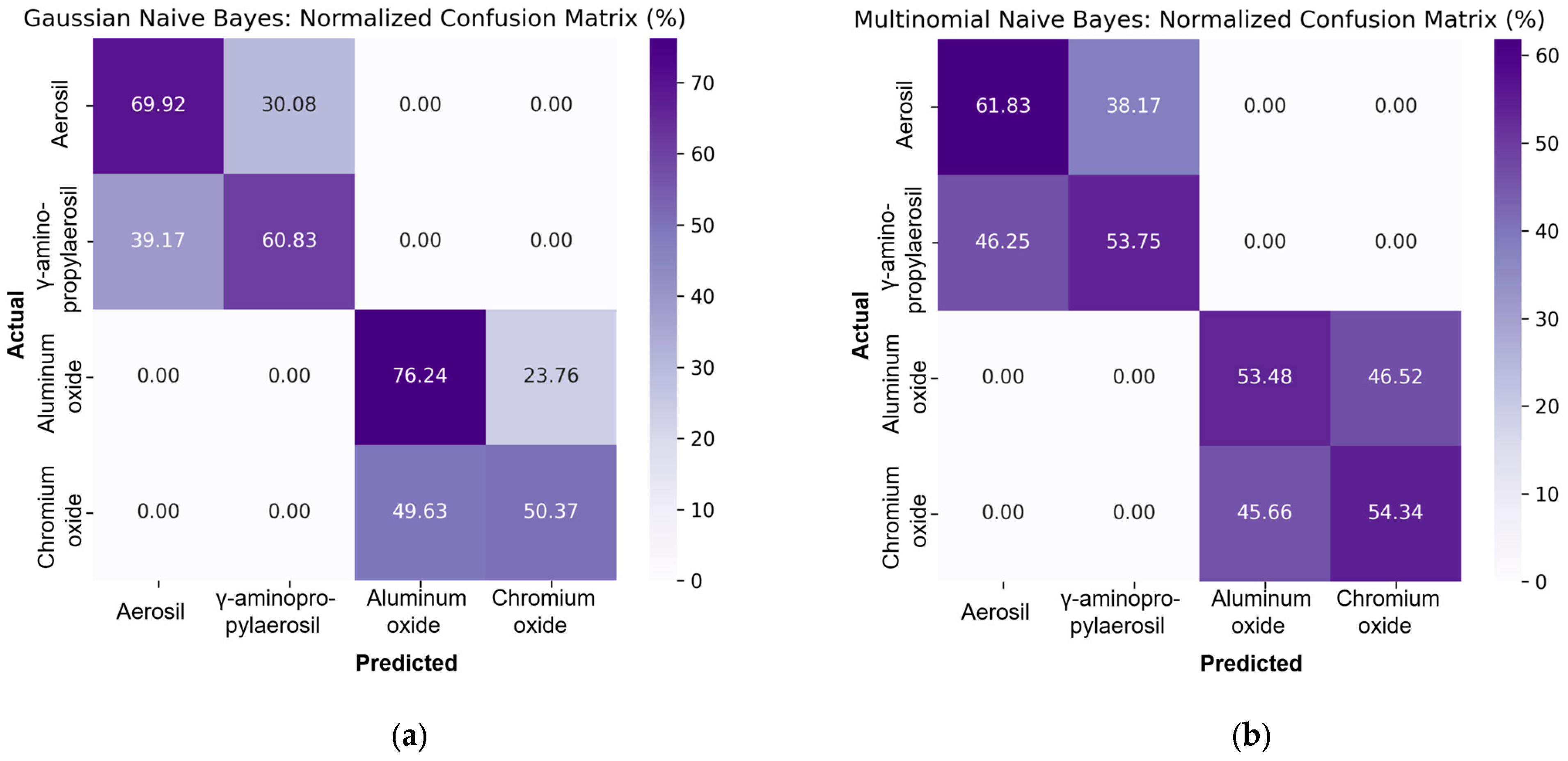
Figure 3 shows the normalized error matrices for the GaussianNB and MultinomialNB models.

The elements of the main diagonal reflect the percentage of correctly classified objects in each class. For the GaussianNB model, the smallest proportion of correct classifications is observed at 50.37%, while for MultinomialNB it is 53.48%. Although MultinomialNB has a slightly higher minimum accuracy within a single class, the overall structure of its matrix indicates less clear class boundaries and significant interclass confusion. In its turn, GaussianNB provides higher classification accuracy in most classes and shows a better ability of the model to detect differences between samples.

Figure 4 shows histograms of confidence levels, which present the distribution of predicted probabilities for correct (blue) and incorrect (red) classifications.

In the case of GaussianNB, it is noticeable that most correct predictions fell within the high confidence range, around 0.7–0.9. Errors also occur at fairly high probabilities. For MultinomialNB, predictions were predominantly concentrated in the range 0.5–0.6, with a significant proportion of them being incorrect. This indicates a low level of model confidence and a limited ability to distinguish correct decisions from incorrect ones. The GaussianNB model shows better consistency between the confidence level and the quality of classification, while MultinomialNB is characterized by less stable probability estimates.

Table 2. Performance indicators of GaussianNB.

Class	TP	TN	FP	FN	Accuracy	Recall	Specificity	Precision	F1-Score	G-Mean
1	839	3147	470	361	0.8274	0.6991	0.8700	0.6409	0.6687	0.7799
2	730	3256	361	470	0.8274	0.6083	0.9001	0.6691	0.6372	0.7400
3	921	3009	600	287	0.8158	0.7624	0.8337	0.6055	0.6749	0.7972
4	609	3321	287	600	0.8158	0.5037	0.9204	0.6796	0.5786	0.6809

and

Table 3. Performance indicators of MultinomialNB.

Class	TP	TN	FP	FN	Accuracy	Recall	Specificity	Precision	F1-Score	G-Mean
1	742	3062	555	458	0.7897	0.6183	0.8465	0.5720	0.5943	0.7235
2	645	3159	458	555	0.7897	0.5375	0.8733	0.5847	0.5601	0.6851
3	646	3057	452	462	0.7687	0.5347	0.8470	0.5392	0.5369	0.6730
4	657	3046	462	452	0.7687	0.5434	0.8442	0.5389	0.5411	0.6773

show the classification metrics for the GaussianNB and MultinomialNB models, which can be used to evaluate their performance.

It has been established that although both models belong to the family of naive Bayesian classifiers and have low computational complexity, GaussianNB is more suitable for this classification task. The F1-score metrics show a better balance between accuracy and completeness for GaussianNB, with a maximum F1 value of 67% compared to 59% for MultinomialNB. Analysis of the geometric mean G-Mean confirms the higher generalization ability of GaussianNB to 80% compared to 72% in MultinomialNB, which indicates a better balance between recall and specificity. Thus, GaussianNB not only outperforms in terms of absolute accuracy, but also shows more stable performance in terms of metrics that take into account the quality of classification at the level of each individual class.

3.2. Results of Linear Classifiers

Optimal hyperparameters of linear classification model were determined using the GridSearchCV method.

In the Logistic Regression model, the best results were achieved for the regularization coefficient C = 1000, which indicates weak regularization, as well as when using the lbfgs optimizer, which ensures stable and efficient work with multi-class tasks. This configuration ensured high classification accuracy. In the Ridge Classifier model, the best results were obtained for alpha = 0.1, which sets the strength of L2 regularization, together with the solver = ‘auto’ parameter, which allows for the automatic selection of the most effective solution algorithm. The value fit_intercept = True was also set without class weight coefficients. This configuration indicates insignificant regularization. After selecting the parameters, the model was wrapped in a calibrator with a sigmoid function, which allowed the use of probabilistic estimates in further analysis. For the SGD classifier, the key parameters were alpha = 0.001, which determines the level of regularization, loss = hinge, which implements a loss function similar to SVM, and penalty = l1, which contributes to the formation of sparse models. The model was trained without class weight coefficients and with the addition of a free term. To improve the quality of probabilistic predictions, the model was also calibrated using the CalibratedClassifierCV wrapper with the sigmoid method. All three models were trained based on cross-validation optimization and adapted for further analysis on the test sample.

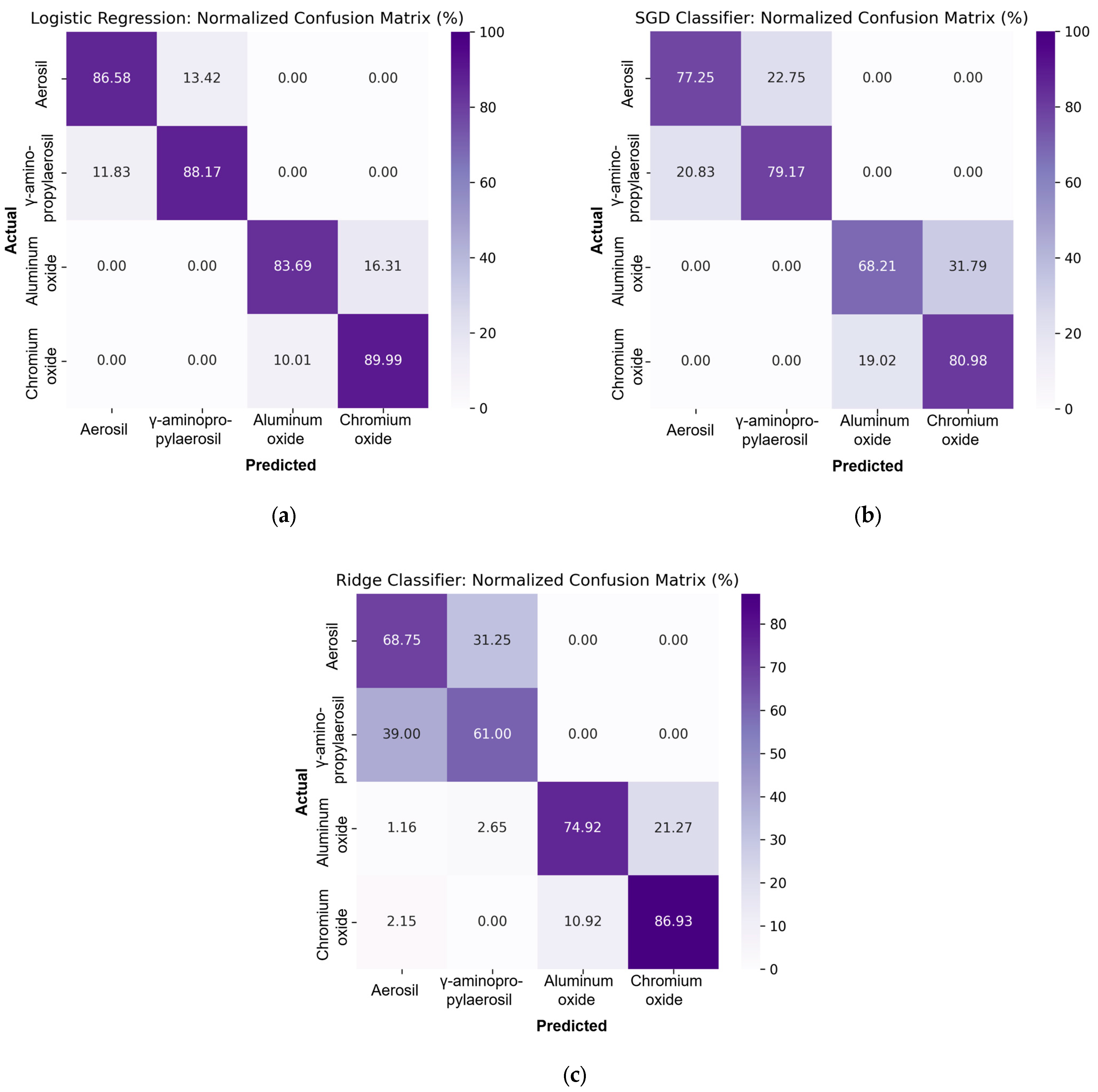
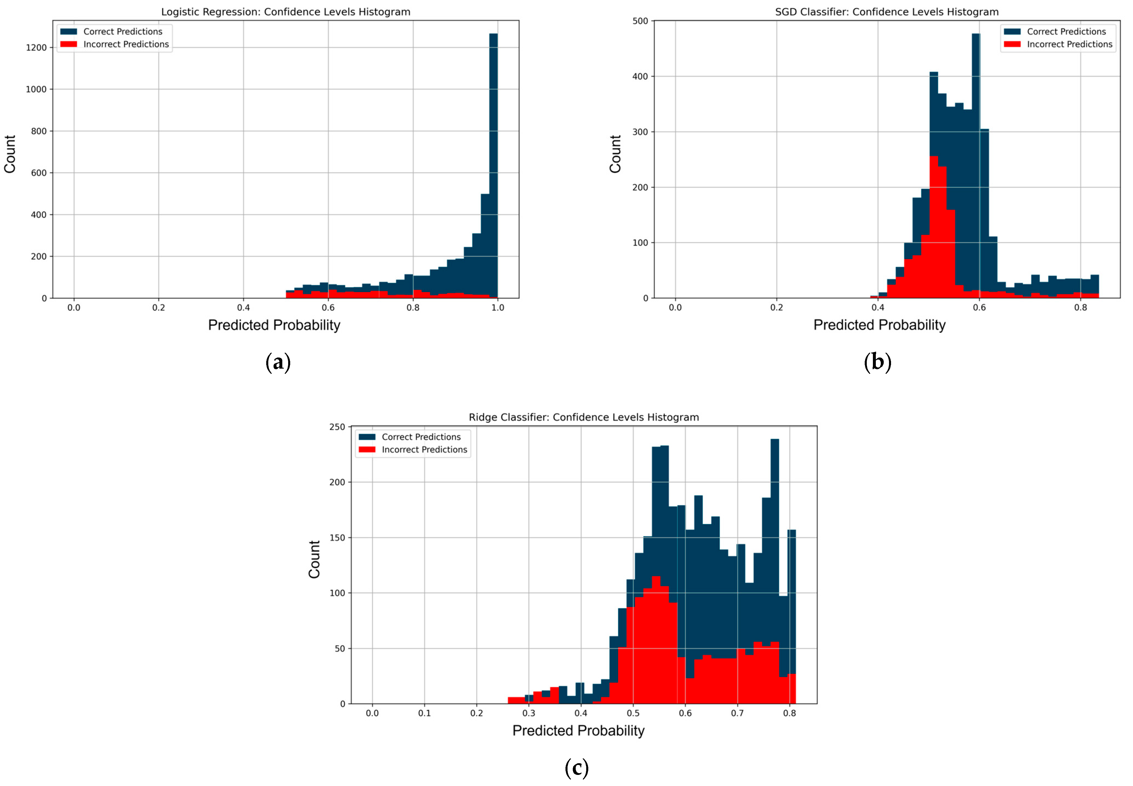
Figure 5 shows normalized confusion matrices for three linear classifiers: Logistic Regression, SGDClassifier, and RidgeClassifier.

It has been established that the Logistic Regression model is the most accurate among the three models, with the lowest percentage of correct classifications at 83.69%. In the case of SGDClassifier, the lowest accuracy is 68.21%. RidgeClassifier shows an even lower minimum accuracy of 61.00%. Thus, among linear models, Logistic Regression has the best overall classification ability, while RidgeClassifier has the worst accuracy values.

Figure 6 shows histograms of model confidence levels. Logistic Regression models are characterized by high confidence in most predictions: correct predictions are concentrated in the range from 0.9 to 1.0, while the proportion of incorrect decisions in this range is insignificant. In the case of SGD Classifier, the confidence of the classifier is within 0.8, with correct and incorrect predictions significantly overlapping in the range of 0.45–0.6. Ridge Classifier shows an even more limited confidence range, within approximately 0.3–0.8, with a significant overlap of correct and incorrect decisions in the central range of 0.5–0.7, confirming the lower reliability of the model’s confidence. Thus, Logistic Regression provides not only the highest confidence levels, but also the best separation between correct and incorrect classifications.

Table 4. Performance indicators of Logistic Regression.

Class	TP	TN	FP	FN	Accuracy	Recall	Specificity	Precision	F1-Score	G-Mean
1	1039	3475	142	161	0.9370	0.8658	0.9607	0.8797	0.8727	0.9120
2	1058	3456	161	142	0.9370	0.8816	0.9554	0.8679	0.8747	0.9178
3	1011	3488	121	197	0.9339	0.8369	0.9664	0.8931	0.8641	0.8993
4	1088	3411	197	121	0.9339	0.8999	0.9453	0.8466	0.8724	0.9223

,

Table 5. Performance indicators of SGDClassifier.

Class	TP	TN	FP	FN	Accuracy	Recall	Specificity	Precision	F1-Score	G-Mean
1	927	3367	250	273	0.8914	0.7725	0.9308	0.7875	0.7799	0.8480
2	950	3344	273	250	0.8914	0.7916	0.9245	0.7767	0.7841	0.8555
3	824	3379	230	384	0.8725	0.6821	0.9362	0.7817	0.7285	0.7991
4	979	3224	384	230	0.8725	0.8097	0.8935	0.7182	0.7612	0.8506

and

Table 6. Performance indicators of RidgeClassifier.

Class	TP	TN	FP	FN	Accuracy	Recall	Specificity	Precision	F1-Score	G-Mean
1	825	3109	508	375	0.8166	0.6875	0.8595	0.6189	0.6514	0.7687
2	732	3210	407	468	0.8183	0.6100	0.8874	0.6426	0.6259	0.7357
3	905	3477	132	303	0.9096	0.7491	0.9634	0.8727	0.8062	0.8495
4	1051	3351	257	158	0.9138	0.8693	0.9287	0.8035	0.8351	0.8985

show the classification metrics for the Logistic Regression, SGDClassifier ta RidgeClassifier.

Analyzing the results of the Logistic Regression, SGD Classifier, and Ridge Classifier models, we can draw a general conclusion about their effectiveness in multi-class classification tasks. Logistic Regression showed stable and high performance across all metrics. High accuracy and a balance between precision and recall for each class prove the reliability of this model. The SGD Classifier model, despite its lower performance, has a sufficient level of classification. In some classes, Ridge Classifier showed the lowest results in terms of accuracy among these three methods, which indicates the model’s insufficient ability to generalize. The F1-score and G-Mean Logistic Regression metrics have the highest values, confirming the balanced performance of the model for all classes. For the SGD Classifier, these metrics are slightly lower but remain acceptable for practical application. The worst results for these metrics were observed in Ridge Classifier, indicating potential difficulties for the model in classifying classes with similar features.

3.3. Results of Support Vector Machines and Nearest Neighbors

In the kNN model, the optimal parameters were selected using the GridSearchCV method, which exhaustively searches through all possible combinations of values. It was found out that the best configuration is n_neighbors = 3 and weights = uniform. This means that for the classification of a new sample, the three closest neighbors with equal weight were taken into account. The model was based on the Euclidean metric (p = 2) in the feature space, which is the standard choice within the Minkowski metric. This configuration ensured good accuracy without the need for weighted voting schemes. GridSearchCV was also used for the SVM model, which allowed us to determine the best hyperparameters from several combinations of kernels, regularization parameters C, and kernel scale gamma. The best parameters are C = 100, kernel = rbf, and gamma = scale. A high C value enhances the role of the penalty coefficient in the loss function, while the radial basis function (RBF) as the kernel provides the model with the ability to construct nonlinear separation boundaries. The value gamma = scale allowed the width of the Gaussian kernel to be automatically adapted to the characteristics of the input data.

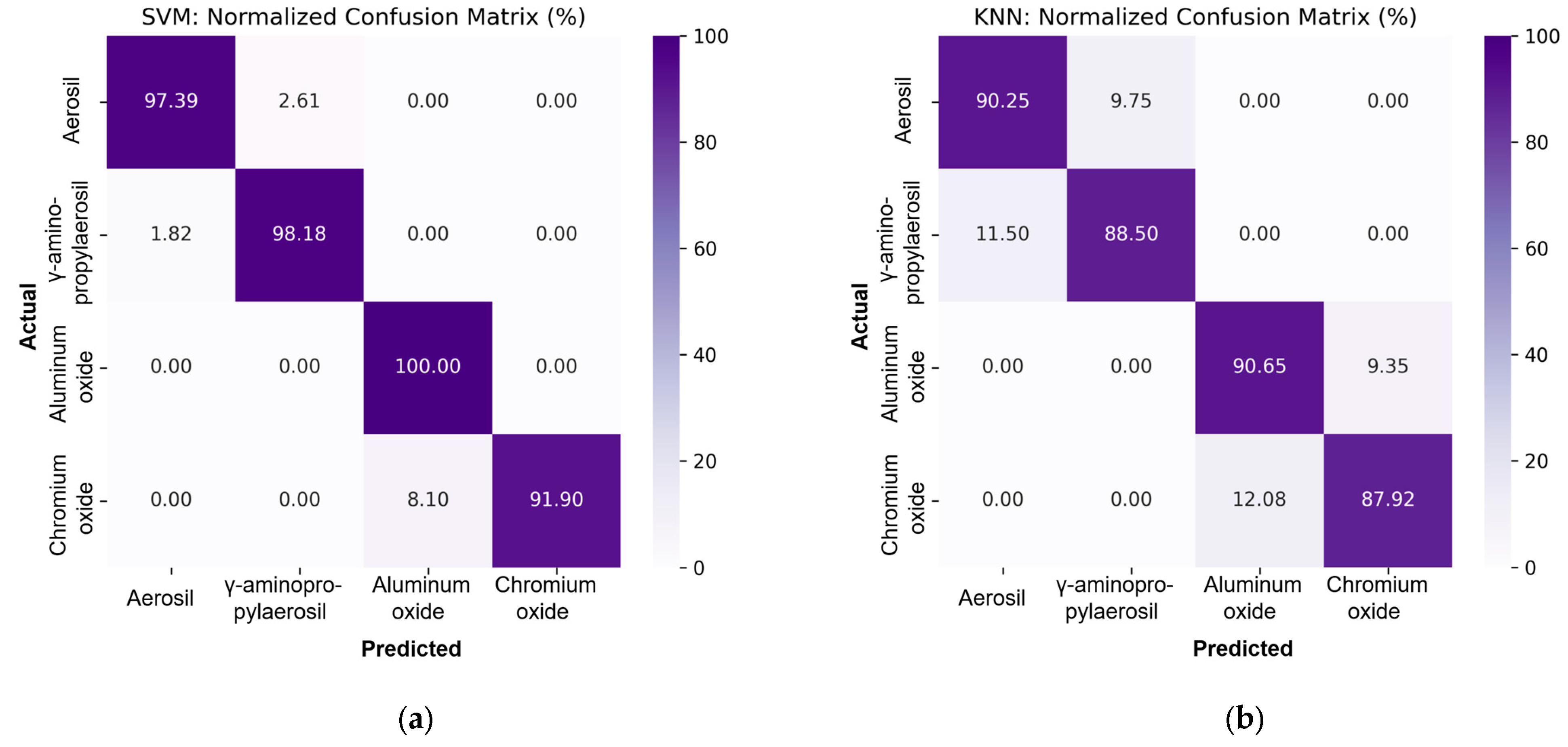
Figure 7 shows the normalized confusion matrices for the SVM and kNN methods.

Both methods showed high classification accuracy, as can be seen from the values on the main diagonal. In the case of SVM, the lowest classification accuracy for classes was 91.90%, confirming the stable performance of the model regardless of class. The kNN method is slightly inferior with a minimum accuracy of 87.92%, but it also provides high classification quality. Thus, both models are capable of providing reliable recognition of filler types in a multi-class task, but SVM shows slightly better consistency across all classes.

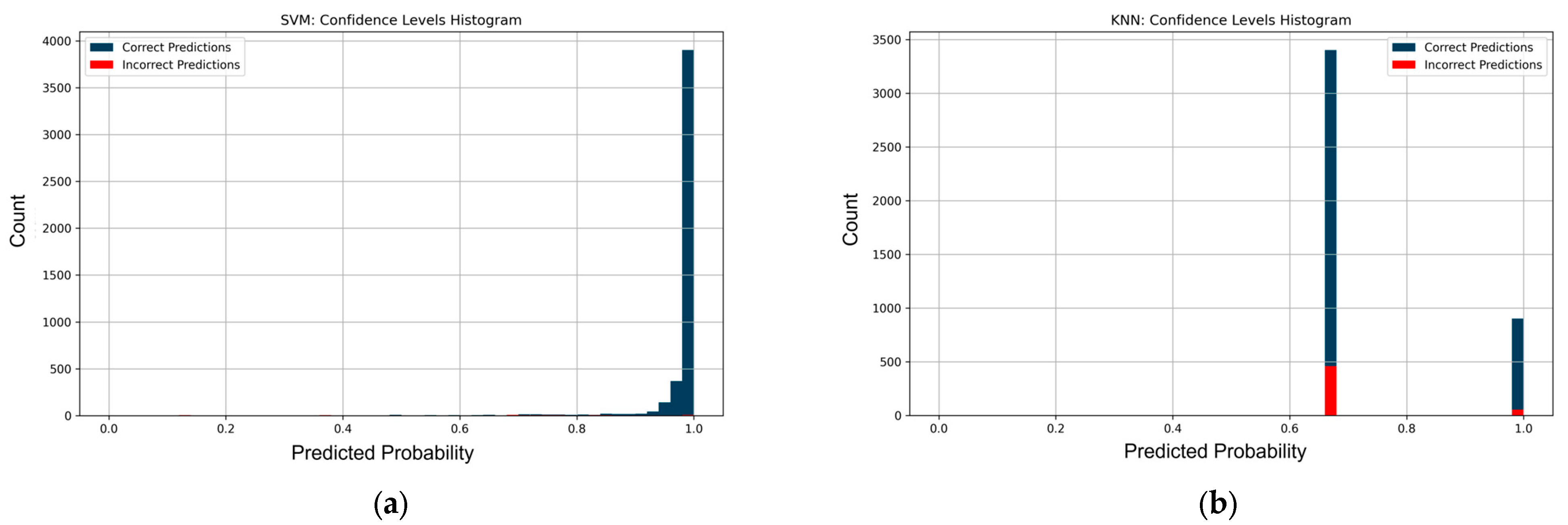
Figure 8 shows the confidence level histograms for the models. For SVM, most correct predictions are concentrated in the area with high confidence values, above 0.95, which indicates the model’s high ability to form unambiguous decisions.

False predictions are possible at lower confidence values, but they have a negligible share. In the case of kNN, there is a peak prediction frequency of about 0.67, which is characteristic of this model due to the specifics of voting among neighbors. At the same time, correct predictions prevail, but there are also a significant number of false decisions, which indicates less stable behavior of the model compared to SVM.

Table 7. Performance indicators of Support Vector Machine.

Class	TP	TN	FP	FN	Accuracy	Recall	Specificity	Precision	F1-Score	G-Mean
1	1159	3605	22	31	0.9889	0.9739	0.9939	0.9813	0.9776	0.9838
2	1185	3579	31	22	0.9889	0.9817	0.9914	0.9813	0.9781	0.9865
3	1260	3463	94	0	0.9804	1.0	0.9735	0.9305	0.9640	0.9866
4	1066	3657	0	94	0.9804	0.9189	1.0	1.0	0.9577	0.9586

and

Table 8. Performance indicators of k-Nearest Neighbors.

Class	TP	TN	FP	FN	Accuracy	Recall	Specificity	Precision	F1-Score	G-Mean
1	1083	3479	138	117	0.9470	0.9025	0.9618	0.8869	0.8946	0.9317
2	1062	3500	117	138	0.9470	0.8850	0.9676	0.9007	0.8928	0.9254
3	1095	3463	146	113	0.9462	0.9064	0.9595	0.8823	0.8942	0.9326
4	1063	3495	113	146	0.9462	0.8792	0.9686	0.9039	0.8914	0.9228

show the main metrics for SVM and kNN models. In particular, both methods provided high accuracy and classification balance.

Analyzing the results of SVM and kNN model classification, it can be noted that both models are highly effective, but the SVM model significantly outperforms kNN in most indicators. The SVM model has extremely high classification accuracy, exceeding 98% for all classes. kNN also showed good results with an accuracy of about 94–95% for all classes, but these values are slightly inferior to the corresponding SVM indicators.

In the SVM model, the F1-score reaches 97% and the G-Mean reaches 98%, which indicates a balanced and highly accurate classification. In the case of kNN, the maximum F1-score value is 89%, and G-Mean is 93%, which, although indicating good classification ability, shows a lower level of consistency between precision and recall compared to SVM. Thus, in the classification task under consideration, the SVM model is more suitable in terms of stability, accuracy, and balance of results.

3.4. Results of Ensemble Methods

All models were optimized using GridSearchCV and five-fold cross-validation, which allowed us to select the optimal hyperparameters to achieve maximum accuracy.

In the CatBoostClassifier model, the best results were obtained with a tree depth of 5, a number of iterations equal to 200, and a learning rate of 0.2. This configuration balanced the complexity of the model with sufficient generalization ability for multi-class classification. In the ExtraTreesClassifier model, the optimal parameters included n_estimators = 100 with no depth limit, min_samples_split = 5, min_samples_leaf = 1, criterion = gini, and bootstrap = False. This combination reduced overfitting due to the shallower depth of the split tree while ensuring sufficient variability of trees in the ensemble. For HistGradientBoostingClassifier, the best parameters were as follows: max_iter = 100, learning_rate = 0.1, max_depth = 10, min_samples_leaf = 2, l2_regularization = 0.0. This configuration reduced log loss and ensured effective generalization without the use of regularization. The following optimal parameters were obtained for the XGBClassifier model: n_estimators = 200, max_depth = 4, and learning_rate = 0.2. The model was configured for multi-class classification using the multi:softprob function and the mlogloss metric.

Figure 9 shows the normalized confusion matrices for ensemble methods.

The lowest accuracy among the four models is 97.60% for HistGradientBoostingClassifier, which is still very high. The highest minimum accuracy is found in XGBClassifier and ExtraTreesClassifier, 97.52% and 97.19%, respectively, and CatBoostClassifier, 98.01%. Thus, all the models considered provide stable and reliable classification.

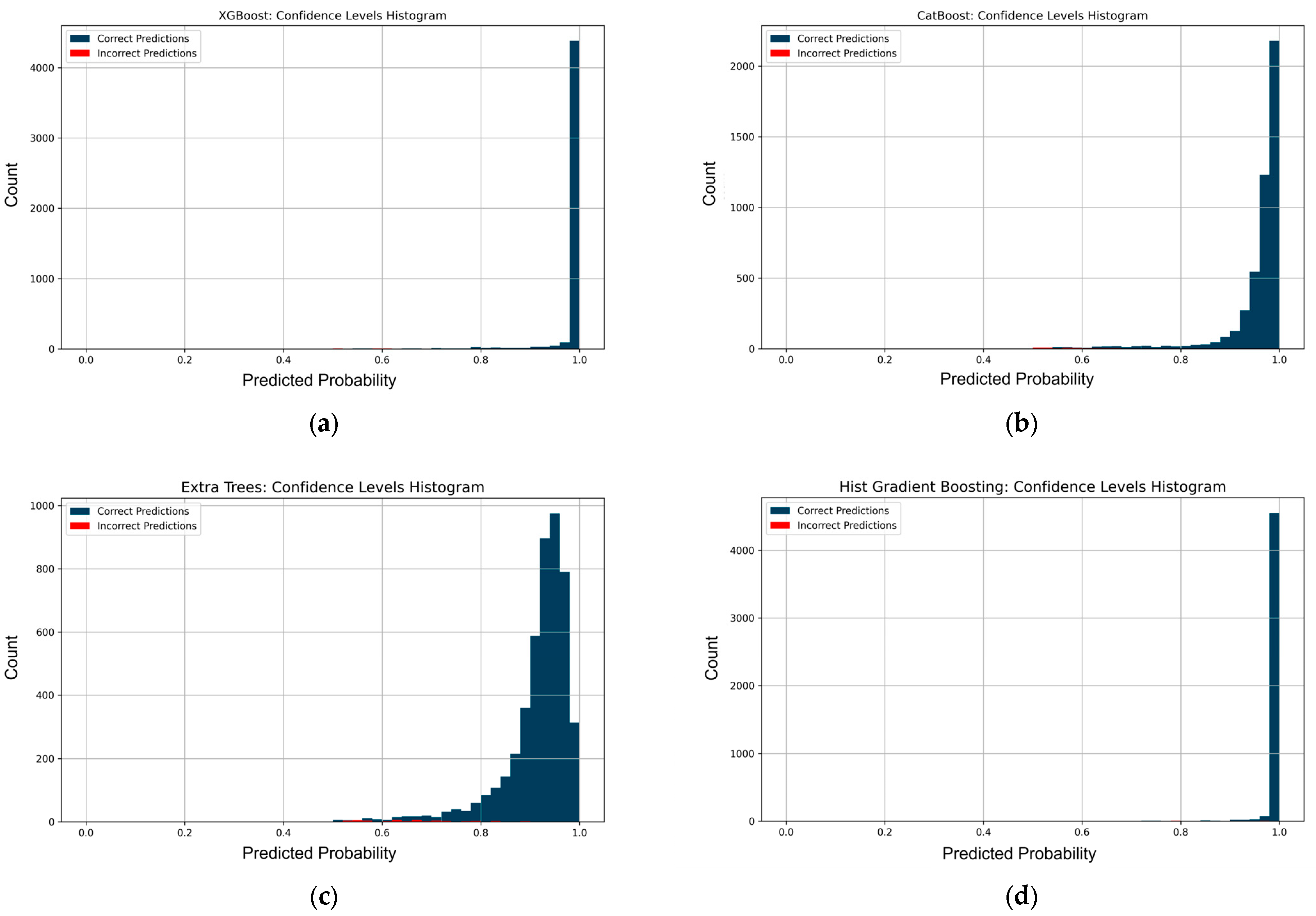
Figure 10 shows the confidence level histograms for these methods. All four models show a high level of confidence with predominantly correct classification in a range close to 1.0. In particular, XGBClassifier has the highest concentration of predictions in a narrow confidence range of 0.98–1.0 with a minimum number of errors. CatBoostClassifier also shows high confidence, but the distribution is slightly wider compared to XGBoost. ExtraTreesClassifier has slightly more confidence dispersion, although most correct predictions are in the range above 0.85. HistGradientBoostingClassifier also shows a very concentrated peak in the maximum confidence zone, similar to XGBoost, with a small number of errors at low confidence levels. Thus, all four models are not only highly accurate but also confident in their predictions, proving their reliability for classification tasks.

Table 9. Performance indicators of XGBClassifier.

Class	TP	TN	FP	FN	Accuracy	Recall	Specificity	Precision	F1-Score	G-Mean
1	1197	3612	5	3	0.9983	0.9975	0.9986	0.9958	0.9966	0.9980
2	1195	3614	3	5	0.9983	0.9958	0.9991	0.9974	0.9966	0.9975
3	1192	3579	30	16	0.9904	0.9867	0.9916	0.9754	0.9810	0.9892
4	1179	3592	16	30	0.9904	0.9751	0.9955	0.9866	0.9808	0.9853

,

Table 10. Performance indicators of CatBoostClassifier.

Class	TP	TN	FP	FN	Accuracy	Recall	Specificity	Precision	F1-Score	G-Mean
1	1193	3609	8	7	0.9968	0.9941	0.9977	0.9933	0.9937	0.9959
2	1192	3610	7	8	0.9968	0.9933	0.9980	0.9941	0.9937	0.9956
3	1191	3585	24	17	0.9914	0.9859	0.9933	0.9802	0.9830	0.9896
4	1185	3591	17	24	0.9914	0.9801	0.9952	0.9858	0.9829	0.9876

,

Table 11. Performance indicators of ExtraTreesClassifier.

Class	TP	TN	FP	FN	Accuracy	Recall	Specificity	Precision	F1-Score	G-Mean
1	1197	3614	3	3	0.9987	0.9975	0.9991	0.9975	0.9975	0.9983
2	1197	3614	3	3	0.9987	0.9975	0.9991	0.9975	0.9975	0.9983
3	1197	3575	34	11	0.9906	0.9908	0.9905	0.9723	0.9815	0.9907
4	1175	3597	11	34	0.9906	0.9718	0.9969	0.9907	0.9812	0.9843

and

Table 12. Performance indicators of HistGradientBoostingClassifier.

Class	TP	TN	FP	FN	Accuracy	Recall	Specificity	Precision	F1-Score	G-Mean
1	1196	3615	2	4	0.9987	0.9966	0.9994	0.9983	0.9974	0.9980
2	1198	3613	4	2	0.9987	0.9983	0.9988	0.9966	0.9975	0.9986
3	1196	3580	29	16	0.9906	0.9867	0.9919	0.9762	0.9814	0.9893
4	1180	3592	16	29	0.9906	0.9760	0.9955	0.9866	0.9812	0.9857

show the performance indicators of the models.

Ensemble models showed excellent classification results, confirming their ability to accurately model dependencies in the analyzed data. They provided high accuracy of over 99% for most classes, with minimal classification error. In particular, the XGBoost and Extra Trees models achieved the highest results and nearly flawless classification, for example, XGBoost: up to 99.83% accuracy with a recall of over 99% and specificity of 99.8%. CatBoost and HistGradientBoosting also showed stable and high-quality predictions with very close values.

Regarding the F1-Score, which takes into account both precision and recall, all four models showed values in the range of 98–99%, which is evidence of balanced classification without significant false positive predictions. The highest F1-Score values were achieved by the XGBoost algorithm at 99.66% and Extra Trees at 99.75%, which emphasizes their high consistency in classification.

The G-Mean indicator is also higher than 98% for all models. This confirms the high stability of recognition for both classes with a small and large number of examples. In XGBoost and Extra Trees, G-Mean reaches 99.8%, confirming the exceptional balance of classification ability.

Therefore, all considered models are suitable for the classification task. The XGBoost and Extra Trees models show a slight advantage over the others, especially due to their high F1-Score and G-Mean with a minimum number of errors.

3.5. Results of Neural Networks of MLP Type

3.5.1. Architecture and Performance Evaluation

In this work, a Multilayer Perceptron neural network was built based on TensorFlow/Keras [111] and optimized using Hyperband automatic tuning, exploring the space of architectures and hyperparameters according to the criterion of maximum validation accuracy. The best configuration contains a sequential stack of four dense blocks: the first layer contains 150 neurons, the second—200, the third—50, and the fourth—150. After each layer, Batch Normalization is applied, which stabilizes the internal distributions of activations, and Dropout with selected coefficients of 0.1, 0.4, 0.2, and 0.0, respectively, which reduces overfitting by stochastically turning off neurons in the training phase. Sparse_categorical_crossentropy was chosen as the loss function. All hidden layers use the nonlinear ReLU activation function. The final layer had four outputs with the softmax activation function, which corresponded to the multi-class classification task.

The selected Adam optimizer worked with an extremely low learning rate of 1 × 10⁻⁶, which Hyperband determined to be the most stable for convergence. The parameters β₁ = 0.9, β₂ = 0.999, and ε = 1 × 10⁻⁷ were set. To combat possible gradient degradation during long-term training, a two-stage training control scheme was used. During the search phase, Hyperband trained each candidate with validation on 10% of the data using an early stopping strategy and accuracy monitoring (val_accuracy) to select hyperparameters. The best obtained model was further trained using early stopping, restoration of the best weights, and dynamic reduction in the learning rate to no less than 1 × 10⁻⁶.

Due to the selection of hyperparameters and a cautious training strategy, the model is able to generalize effectively, achieving the highest accuracy among all the classifiers studied.

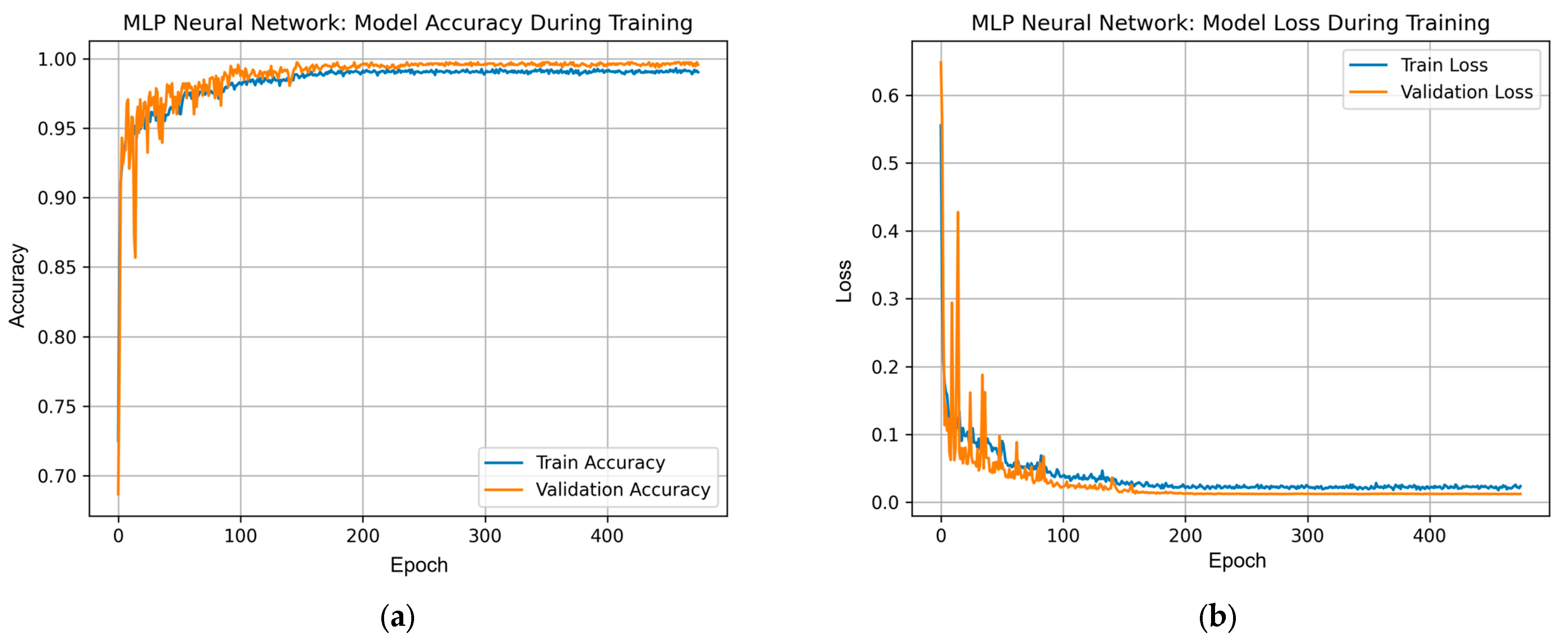
Figure 11 shows the dynamics of the accuracy and loss function of the MLP model during training epochs. As can be seen from the accuracy plot, the model shows stable growth on both the training and validation samples, reaching high values of over 97% after the first 100 epochs. This indicates effective generalization without obvious signs of overfitting. The loss graph confirms the stable behavior of the model—the loss values decrease and remain at a low level after the initial adaptation period. High accuracy on the validation sample with minimal losses indicates balanced model training and its good generalization ability.

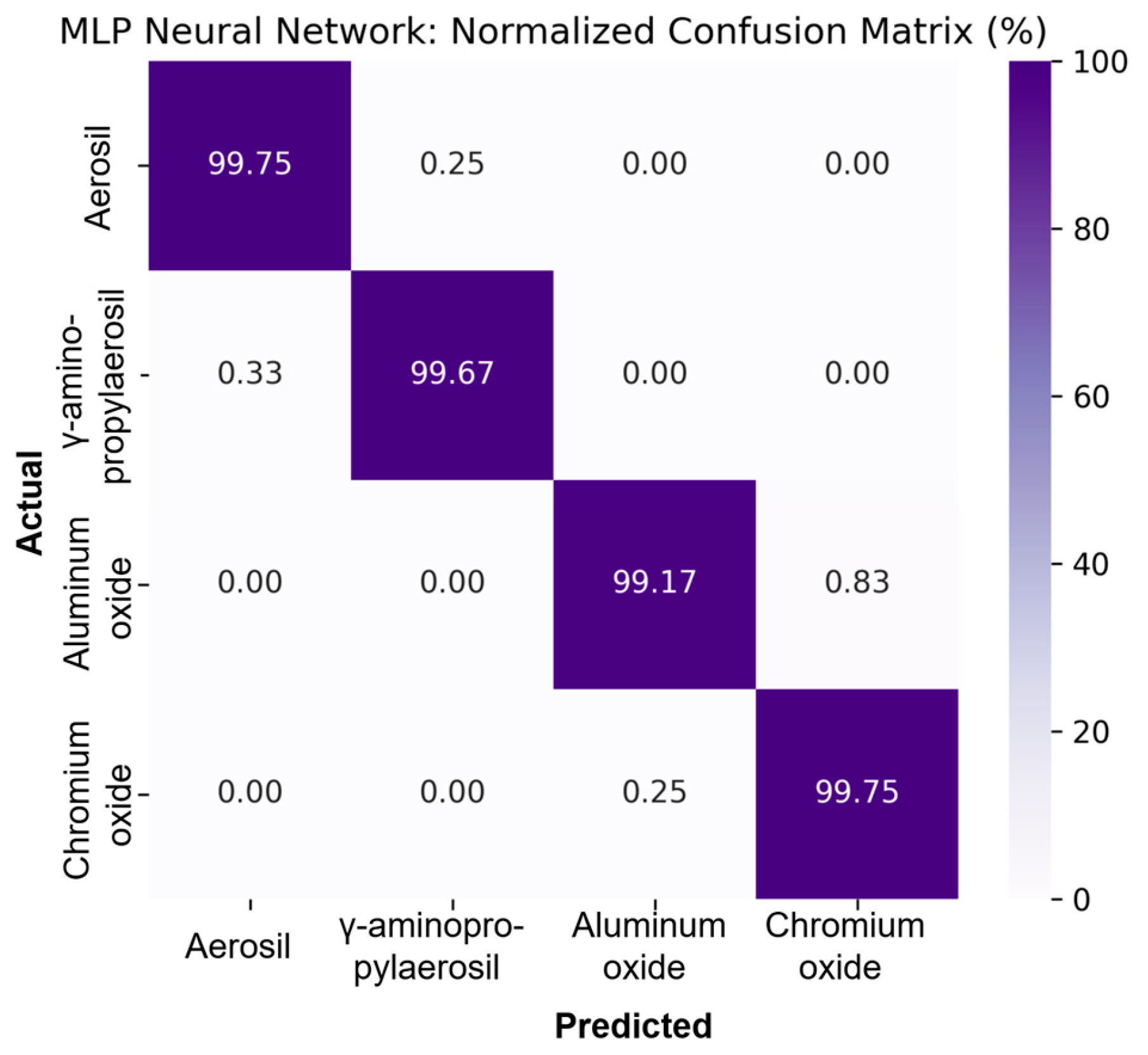
Figure 12 shows the normalized confusion matrix for the MLP model, which has a high classification rate for all four classes. The model correctly classified over 99% of samples in each class, with a minimum accuracy value of 99.17%. This confirms the exceptional ability of MLP to generalize data and provide accurate predictions, even under the complex conditions of multi-class classification. This result exceeds the performance of other models, proving the superiority of neural networks in performing this task.

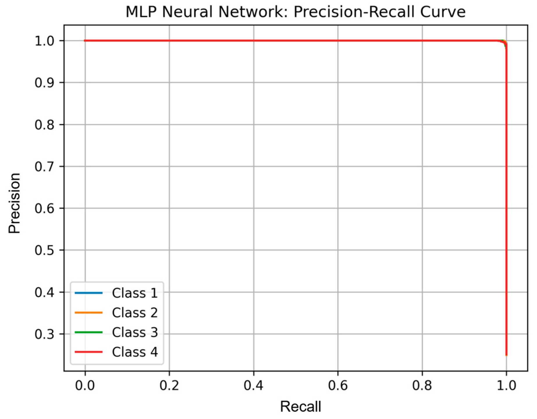
Figure 13 shows the precision-recall curve for each class.

It can be seen that the model shows almost perfect predictions for all four classes. The shape of the curves indicates the model’s high ability to correctly recognize each class with a minimum number of false positives and false negatives. This confirms the effectiveness of training and the generalizing ability of the model.

Figure 14 shows the ROC curves for each of the four classes. All curves pass very close to the upper left corner of the graph, which indicates high classification quality. The AUC area under the curve for all classes exceeds 0.999, which corresponds to an almost perfect classifier. This result indicates that the model accurately separates positive and negative samples of each class even when the classification threshold changes.

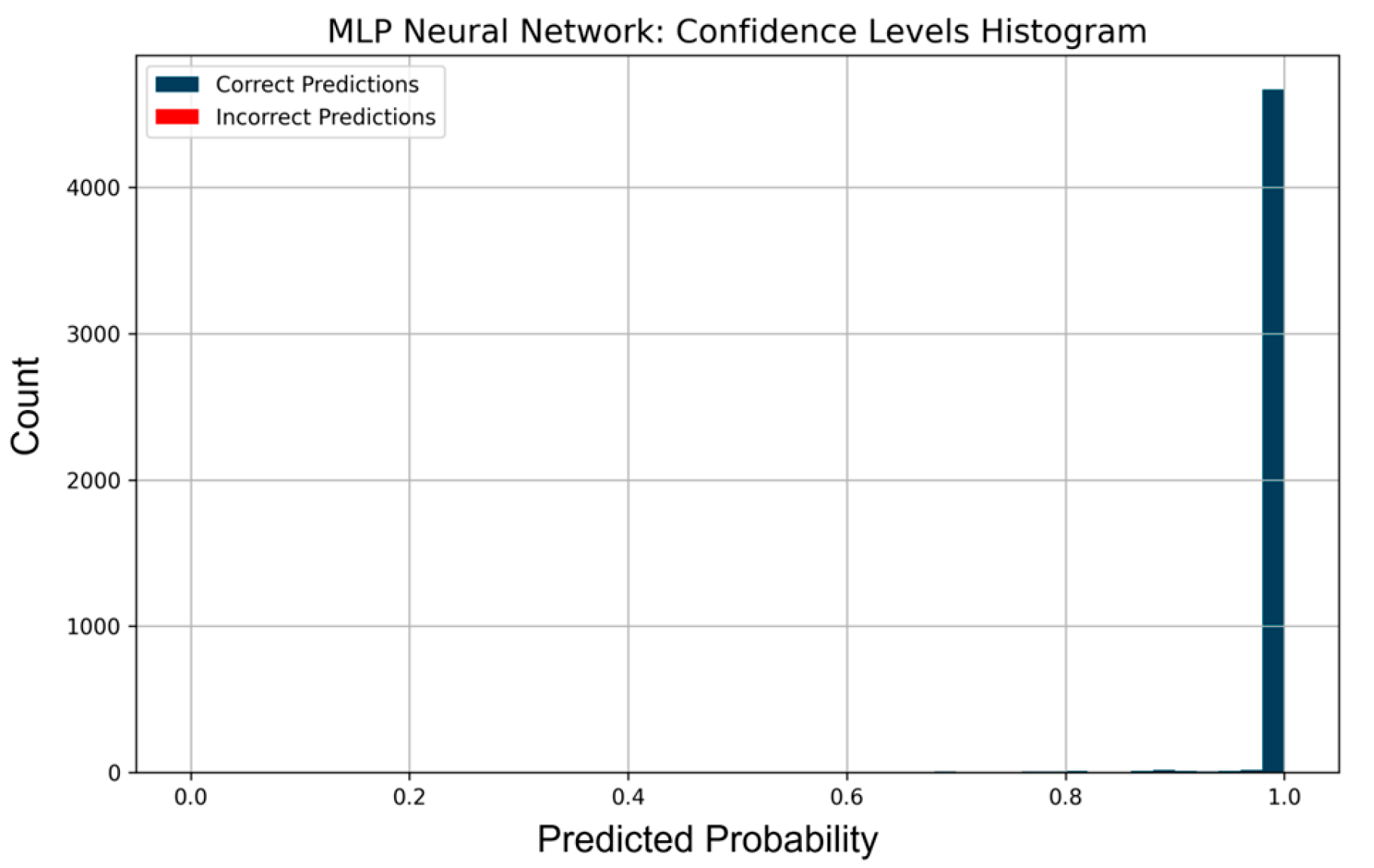
Figure 15 shows a histogram of the confidence levels of the MLP model.

It can be seen that the vast majority of correct predictions are concentrated in the confidence range close to 1.0. This indicates the model’s high confidence in classification decisions. The red columns corresponding to false predictions are almost absent, which is another indicator of the model’s high accuracy. This pattern is characteristic of well-trained neural networks, which demonstrate both confidence and accuracy in decision-making, especially when there is sufficient data for training.

Table 13. Performance indicators of MLP.

Class	TP	TN	FP	FN	Accuracy	Recall	Specificity	Precision	F1-Score	G-Mean
1	1197	3613	4	3	0.9985	0.9975	0.9988	0.9966	0.9970	0.9981
2	1196	3614	3	4	0.9985	0.9966	0.9991	0.9974	0.9970	0.9979
3	1198	3606	3	10	0.9973	0.9917	0.9991	0.9975	0.9946	0.9954
4	1206	3598	10	3	0.9973	0.9975	0.9972	0.9917	0.9946	0.9973

shows the main metrics of the MLP model.

The neural network provides extremely high classification quality. All classes are classified with an accuracy of over 99.7%, which proves the exceptional consistency between predictions and actual labels. High Recall and Specificity values confirm that the model performs equally well in detecting both positive and negative examples, with a minimum number of false predictions. In the context of F1-Score, the values range from 99.46% to 99.71%, indicating a very balanced classification. The G-Mean indicator, which summarizes the balance between Recall and Specificity, exceeds 99.5% in all cases, emphasizing the extremely high stability of the model in interclass classification.

The MLP neural network provided the best results among all models, combining high accuracy, consistency, and stability in all metrics. This indicates the effective adaptation of the architecture to the characteristics of the input features and the classification task being solved.

3.5.2. Interpretation Based on the SHAP Algorithm

SHAP analysis is a modern approach to explaining machine model decisions based on Shapley values from cooperative game theory [112,113]. The method allows us to quantitatively assess the contribution of each input feature to the formation of a specific forecast, while preserving the properties of additivity and local accuracy. In the context of this work, SHAP is used for a deeper interpretation of the MLP model results. In the present study, the characteristics of the composite (thermal conductivity coefficient, filler concentration, or temperature) were analyzed to determine which characteristics have the greatest influence on determining the type of filler. SHAP analysis of the saved MLP model was performed on the original, uninterpolated experimental data (Table 1) to reflect the real contribution of each feature to the model’s decision.

Figure 16 shows the importance rating of the input features for the MLP model. It can be seen that the MFFC feature has the highest average value and, accordingly, is a key classification factor. The second most influential factor is the thermal conductivity coefficient TCC, while the least important factor is the temperature T. This indicates that the model is mainly focused on the composition of the material and its conductivity, while temperature plays a secondary role in the classification process.

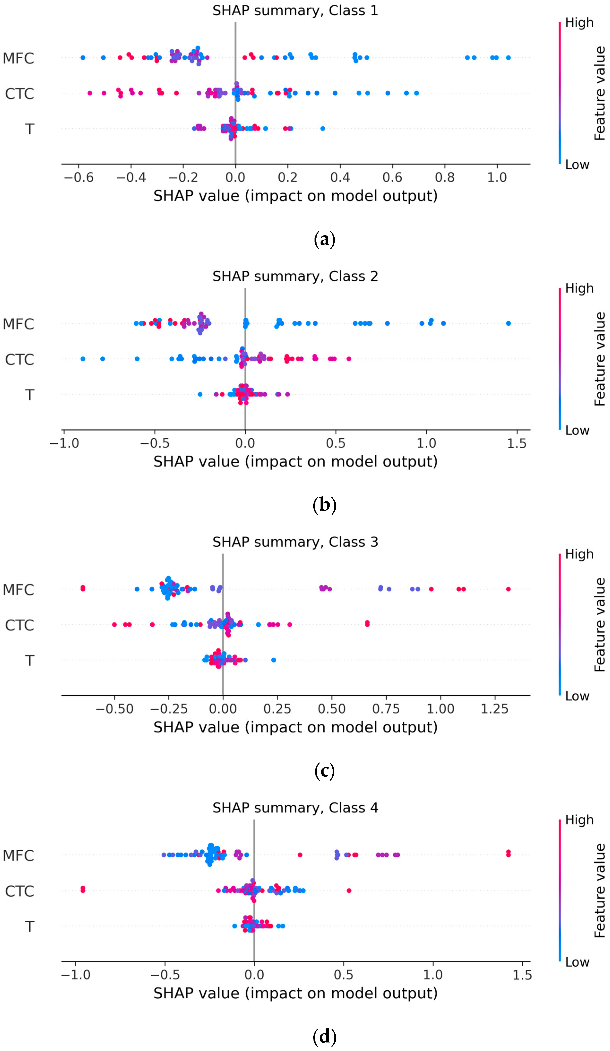
Although Figure 16 shows the relative influence of each feature on the classification results, it does not allow us to assess the direction of this influence. To overcome this limitation, Figure 17 shows SHAP summary plots for each of the four classes, illustrating both the magnitude and direction of the influence of each feature on the probability of belonging to each class.

The SHAP summary plots for each of the four classes show how the values of three features, that is, MFFC, TCC, and T, shift the model output toward increasing or decreasing the probability of the selected class. The horizontal axis shows the magnitude of the influence (SHAP value). On the right is the contribution in favor of the current class, and on the left, against it. In each of the figures, each point corresponds to a separate example from the sample, and with a significant number of overlaps, the points are randomly shifted vertically for better visualization of density. The left vertical axis indicates the feature names, sorted by decreasing impact, according to the ranking in Figure 16, and the right vertical scale encodes the feature values by color, from blue for low values to red for high values.

The plots show that the clusters of points for the mass fraction of filler and the thermal conductivity coefficient extend significantly further from the zero vertical axis than the temperature points, which clearly confirms the predominant role of the first two characteristics in all classes. Points colored in red shades indicate high values of the feature; their location to the right or left of the zero axis immediately shows whether the increase in this feature strengthens or weakens the sample’s belonging to a particular class. For example, for class 1, the blue MFFC points (low concentration) are predominantly shifted to the right, while the red ones are shifted to the left, so the model associates this class with a low filler content. For class 3, the opposite pattern is observed: high MFFC and TCC values (red dots) have positive SHAP contributions, indicating a relationship between the third type of filler and increased concentration and thermal conductivity. Temperature, on the other hand, forms a compact cluster around zero and hardly shifts the model output, which is consistent with its global importance. Thus, the SHAP summary confirms that the model builds decisions based primarily on mass fraction and thermal conductivity, and the direction of their influence differentiates classes, clearly reflecting physical trends in the experimental data.

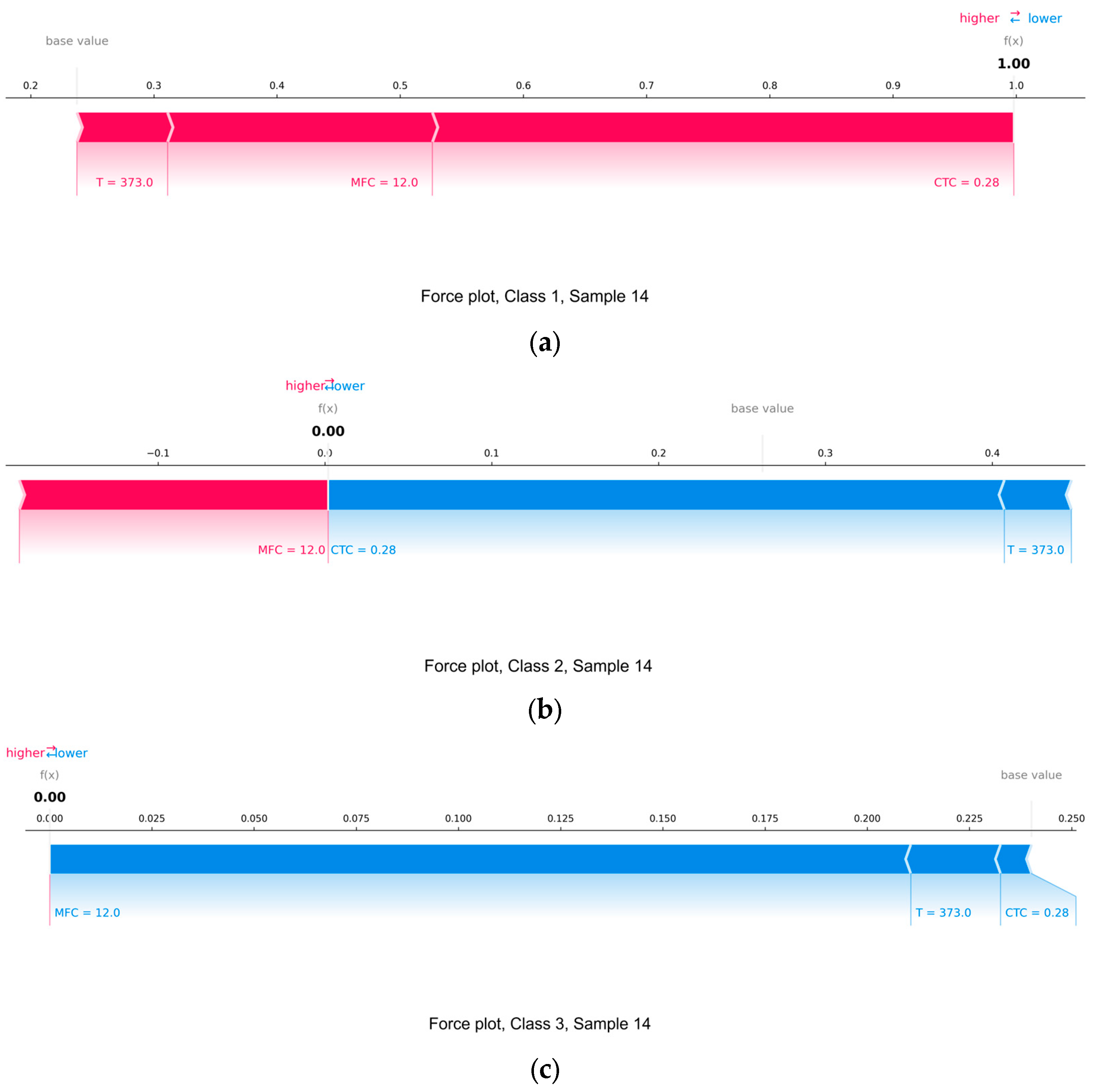
In contrast to SHAP summaries, which summarize the behavior of the model for all samples, SHAP force plots allow us to analyze in detail the impact of each feature on a specific model decision for an individual sample. Figure 18 provides an explanation for the same sample, specifically sample 14, for each of the four classes.

Blue arrows indicate features that decrease the likelihood of being assigned to a class, while red arrows indicate those that increase it. The magnitude of the arrow reflects the strength of the influence. The results are presented as a shift from the baseline average logit output to the predicted logit for each class. Figure 18a shows the SHAP force plot for class 1. TCC and MFFC contributed the most to increasing the classification probability, shifting the model to a logit of ≈0.998. The temperature also contributed to the positive decision, albeit with less influence. All features worked in concert, leading to almost complete confidence in the model that the sample belonged to class 1. Figure 18b shows the situation for class 2. In this case, TCC had a significant negative impact, significantly reducing the probability of the sample belonging to this class. Despite the positive contribution of MFFC, its effect was unable to compensate for the negative effect, and the temperature contributed to an even greater reduction in logit. As a result, the model effectively rejected class 2 for this sample. In Figure 18c, which refers to class 3, there is a strong negative influence of MFFC, as well as weak negative contributions from T and TCC. No feature supported classification to this class, and the final probability was negligible, approximately 0.000014. This result clearly indicates that the model excludes class 3 as relevant for this observation. Figure 18d illustrates the situation for class 4. As in the case of class 3, all features, in particular MFFC and TCC, made a negative contribution, leading to another rejection of the sample from this class. The logit value was reduced compared to the baseline value, and temperature, although with a negligible effect, also reduced the probability of assigning the sample to this class.

In general, SHAP force plots for a specific example confirm the previously identified trend that the MLP model classifies the sample into class 1 with high confidence, based mainly on TCC and MFFC values. For the remaining classes, these same features, changing the direction of influence, reduce the corresponding logits.

4. Conclusions

There were proposed the models capable of classifying the type of filler (aerosil, γ-aminopropylaerosil, Al₂O₃, Cr₂O₃) in basalt-reinforced epoxy composites based on their thermophysical and mechanical characteristics, in particular, the thermal conductivity coefficient, mass fraction of the filler concentration, and temperature, using machine learning methods.

The study confirmed the feasibility and high efficiency of using machine learning methods to classify epoxy composites based on their thermophysical properties. According to the simulation results, the best classification quality was provided by an MLP neural network, which achieved the highest values of accuracy, F1-measure, and G-Mean; in particular, the smallest proportion of correct classifications among all classes was 99.17%. Ensemble methods also showed high performance: XGBoost 97.52%, CatBoost 98.01%, Extra Trees 97.19%, HistGradientBoosting 97.60%. The SVM and kNN methods were slightly less accurate but quite stable, with a minimum accuracy of 91.90% and 87.92%, respectively. Among linear classifiers, Logistic Regression was the best with 83.69%, while SGDClassifier and RidgeClassifier achieved only 68.21% and 61.00%. The worst results were observed in naive Bayes models: GaussianNB 50.37% and MultinomialNB 53.48%.

The application of SHAP analysis made it possible to interpret the decision-making logic of the MLP model and confirmed the key role of the mass fraction of the filler in forming predictions, as well as revealed the class-dependent specificity of the influence of other features. In general, these methods were systematically applied for the first time to the task of classifying filler types based on thermal conductivity coefficient, temperature, and mass fraction of the filler concentration. The use of experimental data interpolation made it possible to achieve high model accuracy even with a limited amount of experimental data. This highlights the potential of machine learning methods in materials science as tools for accurate classification and in-depth analysis of composite properties.