Quasi-LPV Approach for the Stabilization of an Innovative Quadrotor

Abstract

In recent decades, the deployment of quadcopters has significantly expanded, particularly in outdoor applications such as parcel delivery. These missions require highly stable aerial platforms capable of maintaining balance under diverse environmental conditions, ensuring the safe operation of both the drone and its payload. This paper focuses on the stabilization of a quadcopter designed for outdoor use. A detailed dynamic model of a compact vertical takeoff and landing (VTOL) drone forms the basis for a non-linear control strategy targeting stability during the critical takeoff phase. The control law is designed using a quasi-linear parameter-varying (quasi-LPV) model that captures the system’s non-linear dynamics. Lyapunov theory and linear matrix inequalities (LMIs) are employed to validate the stability and design the controller. Numerical simulations demonstrate the controller’s effectiveness, and a comparative study is conducted to benchmark its performance against a reference quadrotor model.

1. Introduction

Quadcopters, a subcategory of small unmanned aerial vehicles (UAVs), have gained remarkable traction in a variety of civilian sectors, including emergency rescue operations, structural monitoring, infrastructure inspection, environmental surveying, and parcel delivery. The increased interest in these platforms stems from their unmatched agility and capability to hover precisely over designated target areas, a feature not easily achievable by fixed-wing aircraft. Additionally, quadcopters can operate in constrained environments, further broadening their utility in urban and confined spaces.

To effectively fulfill such missions, quadcopters must be both compact and highly autonomous, integrating advanced control systems capable of maintaining stability in the presence of disturbances. UAVs can be classified into four broad aerodynamic configurations: fixed-wing, rotary-wing, airships, and flapping-wing designs. Fixed-wing drones typically require a runway and are optimized for long-distance travel, whereas rotary-wing drones are preferred for vertical takeoff and landing (VTOL), hover capabilities, and superior maneuverability. Airship-type drones function similarly to balloons, offering long endurance but limited control authority, while flapping-wing drones, inspired by biological flight mechanisms, excel in micro-scale flight scenarios. Other innovative drone architectures have been proposed recently, notably by Modi et al. [1], where the configuration of the drone dynamically adapts depending on the assigned task.

In this study, our attention is focused on the design and control of a novel quadcopter architecture known as XSF, developed at the University of Évry–Paris-Saclay. The XSF quadrotor is uniquely characterized by two pivoting rotors, enabling it to perform translational movements without altering its attitude—an innovation that differentiates it from conventional cross-rotor configurations. The traditional quadcopter, despite being a subject of extensive research [2,3,4], still presents challenges related to stabilization and control in the presence of non-linear dynamics and exogenous disturbances.

The scope of potential applications for quadcopters continues to expand, encompassing not only aerial surveillance and remote sensing but also tasks such as detailed inspection of complex structural geometries (e.g., bridge underbellies and irregular façades), indoor facility monitoring (e.g., tanks or pipes), and precision agriculture. Recent studies, such as [5], have highlighted the integration of visual navigation systems and image recognition to enhance the autonomy and adaptability of quadrotor UAVs in dynamic environments. Despite these technological advancements, quadcopters remain vulnerable to instabilities arising from non-linear flight dynamics and the difficulty of obtaining complete state measurements, particularly under turbulent atmospheric conditions.

Addressing these issues necessitates the development of accurate dynamic models and advanced non-linear control strategies that ensure robust stability and trajectory tracking. Incorporating such models into control design frameworks facilitates the formulation of high-performance controllers capable of adapting to real-time system variations. Notable contributions in this domain include the work by Richter et al. [6], which exemplifies model-based control synthesis for UAVs.

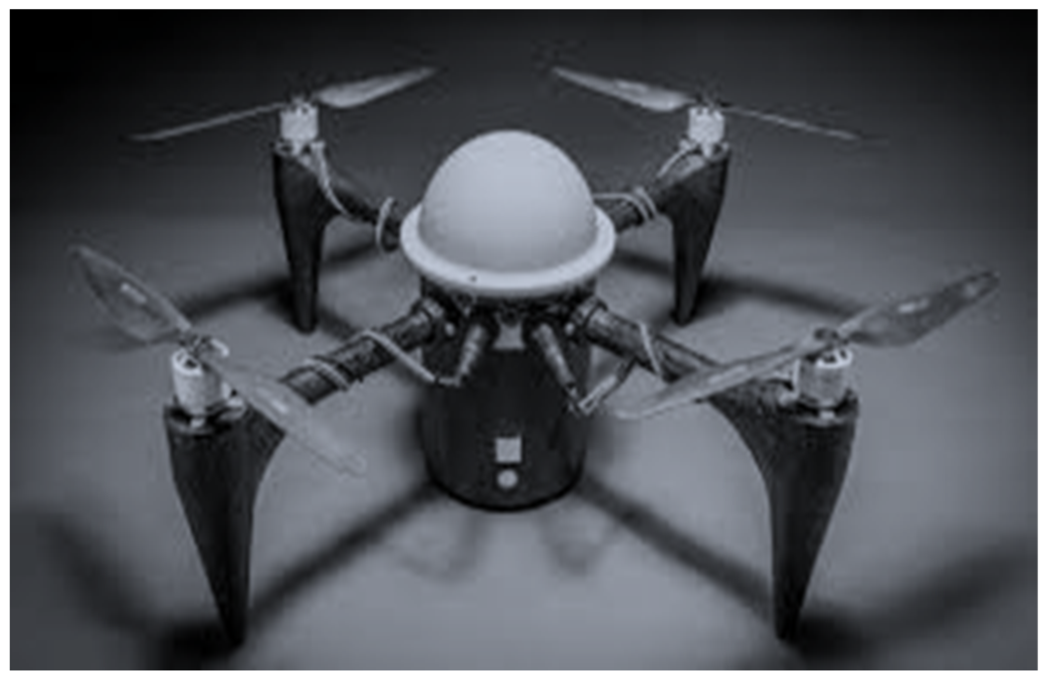
The XSF drone used in this research (illustrated in Figure 1) is an in-house prototype conceived at the University of Évry–Paris-Saclay. Its distinguishing feature—dual directional rotors—grants it the unique ability to translate horizontally without inducing a change in orientation, thereby enabling novel flight modes and enhancing its utility in constrained environments.

The primary objective of this study is to develop and validate a robust control strategy to stabilize this unconventional quadrotor configuration. Prior works, such as [7,8,9], have employed control techniques including backstepping and sliding mode control to stabilize conventional UAVs. Other significant contributions include the study by Xuan-Mung et al. [10], which explores similar control methodologies.

Given the increasing prominence of linear parameter-varying (LPV) modeling techniques [11,12,13], numerous studies have explored state feedback control within this framework, often leveraging the H-infinity (H∞) norm to ensure robustness against disturbances [14]. Recent advancements in quadrotor LPV control [10,15,16,17] have adopted a unified design paradigm centered on the Bounded Real Lemma (BRL), which is used to minimize the H∞ norm and guarantee robust performance. These approaches frequently incorporate Lyapunov-based inequalities to formalize time-domain performance requirements and establish stability guarantees.

In our approach, we employ a polytopic modeling technique that captures the non-linear nature of the system while enabling controller synthesis via interpolation across a set of linearized models. This strategy aligns with the quasi-LPV methodology, which has gained traction in recent studies [13,14,15,16,17,18] for its ability to extend the domain of attraction and preserve non-linear system characteristics. For instance, Coutinho et al. [14] proposed an event-triggered control design using quasi-LPV models, while Baocang et al. [15] examined robust model predictive control for systems affected by bounded disturbances.

Our research focuses specifically on the stabilization of the XSF quadrotor during the takeoff phase—a highly non-linear and sensitive flight regime. Due to its unique geometry and dynamic properties, conventional control methods prove insufficient, necessitating a tailored quasi-LPV-based solution to ensure performance and stability. The success of this approach depends critically on the precision of the dynamic model; therefore, we rely on the aerodynamic and dynamic modeling framework presented in [19] to underpin the design of our control algorithm.

2. The XSF Quadcopter

2.1. Presentation and Description of the Quadcopter

Presentation and description of the quadcopter

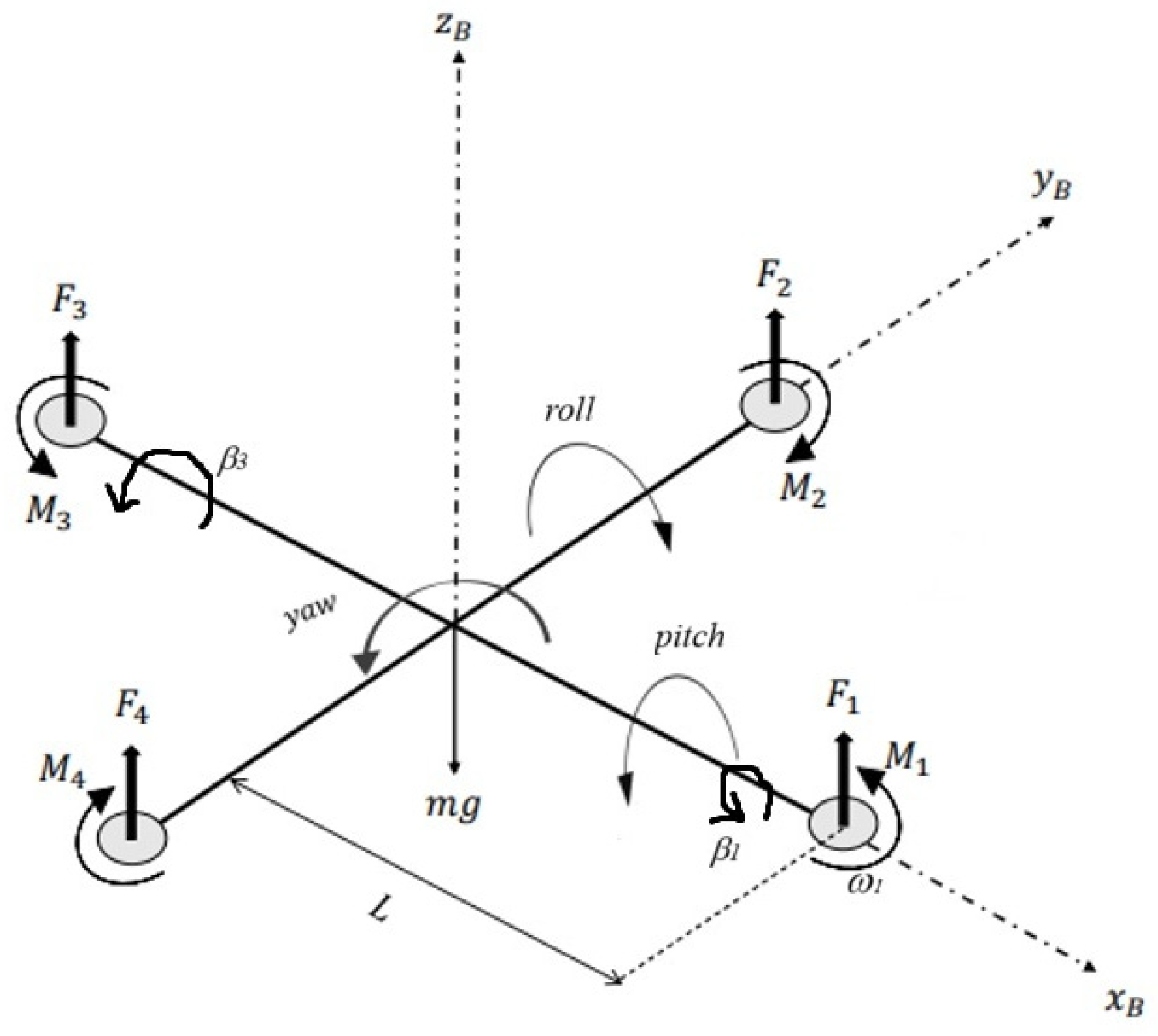
A distinguishing feature of the XSF, unlike traditional quadrotors, is its ability to pivot motors (1) and (3) about the body pitch axis x_B (see Figure 2). This actuation scheme allows the drone to perform efficient horizontal flight maneuvers while enhancing control authority in yaw dynamics.

Note that the angles ${\beta }_1$ and ${\beta }_3$ are the two pivot angles of rotors 1 and 3.

The coefficients K_T and K_M are, respectively, the thrust and drag coefficients determined experimentally, and ω_i is the angular velocity of the rotor i, such that the thrust forces F_i and drag torques M_i are defined as follows:

$$F_i=K_T{\omega }_i^2;\hspace{1em}{M}_i=K_M{\omega }_i^2$$

2.2. Kinematics

One can see in Figure 2 a reduced model of the drone XSF. This last one is assumed to be a rigid flying object. In aeronautics the parameterization in yaw, pitch, and roll (ψ, θ, and φ) is used to describe the orientation of the moving frame R_B in regard to the inertial frame R₀.

The global kinematic equation of the airship is given by the following [20]:

$$\dot{\eta }=\left(\begin{array}{cc}{J}_1({\eta }_2)& 0\\ 0& J_2({\eta }_2)\end{array}\right)\left(\begin{array}{l}{\nu }_1\\ {\nu }_2\end{array}\right)$$

(1)

with

$$J_1({\eta }_2)=\left(\begin{array}{ccc}c\theta .c\psi & s\varphi .s\theta .c\psi -c\varphi .s\psi & c\varphi .s\theta .c\psi +s\varphi .s\psi \\ c\theta .s\psi & s\varphi .s\theta .s\psi +c\varphi .c\psi & c\varphi .s\theta .s\psi -s\varphi .c\psi \\ -s\theta & s\varphi .c\theta & c\varphi .c\theta \end{array}\right)$$

(2)

such that $J_1{({\eta }_2)}^T{J}_1({\eta }_2)=J_1({\eta }_2)J_1{({\eta }_2)}^T=I_3$; we will note $s\varphi =\sin \varphi$ and $c\theta =\cos \theta$.

Subsequently, the kinematic equations may be derived as follows:

$$\left\{\begin{array}{l}{\dot{x}}_0=c\theta .c\psi .u+(s\varphi .s\theta .c\psi -c\varphi .s\psi )v+(c\varphi .s\theta .c\psi +s\varphi .s\psi )w\\ {\dot{y}}_0=c\theta .s\psi .u+(s\varphi .s\theta .s\psi +c\varphi .c\psi )v+(c\varphi .s\theta .s\psi -s\varphi .c\psi )w\\ {\dot{z}}_0=-s\theta .u+s\varphi .c\theta .v+c\varphi .c\theta .w\end{array}\right.$$

(3)

and $J_2({\eta }_2)$ is the matrix relating the rotation speeds such that

$$\left\{\begin{array}{l}\dot{\varphi }=p+s\varphi .\tan \theta .q+c\varphi .\tan \theta .r\\ \dot{\theta }=c\varphi .q-s\varphi .r\\ \dot{\psi }={\displaystyle \frac{s\varphi }{c\theta }}q+{\displaystyle \frac{c\varphi }{c\theta }}r\end{array}\right.$$

(4)

2.3. Dynamics

The XSF drone is modeled first as a rigid flying object. We use here an Eulerian approach, while a Lagrangian approach can be seen in [3,21].

By introducing the aerodynamic forces and torques, we can give the complete dynamic model of an XSF drone [19]:

$$\left\{\begin{array}{l}\dot{u}=rv-qw-g.s\theta -{\displaystyle \frac{K_T}{m}}({\omega }_1^2\mathrm{s}{\beta }_1+{\omega }_3^2\mathrm{s}{\beta }_3)\\ \dot{v}=-ru+pw+g\mathrm{s}\varphi .\mathrm{c}\theta \\ \dot{w}=g.c\varphi .c\theta -pv+qu-{\displaystyle \frac{K_T}{m}}({\omega }_1^2\mathrm{c}{\beta }_1+{\omega }_2^2+{\omega }_3^2\mathrm{c}{\beta }_3+{\omega }_4^2)\\ \dot{p}=-{\displaystyle \frac{l_b{K}_T}{I_{xx}}}({\omega }_1^2\mathrm{c}{\beta }_1-{\omega }_3^2\mathrm{c}{\beta }_3)-{\displaystyle \frac{I_{zz}-I_{yy}}{I_{xx}}}rq-q{\displaystyle \frac{I_R}{I_{xx}}}({\omega }_1\mathrm{c}{\beta }_1+{\omega }_2+{\omega }_3\mathrm{c}{\beta }_3+{\omega }_4)\\ \dot{q}={\displaystyle \frac{l_b{K}_T}{I_{yy}}}({\omega }_2^2-{\omega }_4^2)-{\displaystyle \frac{I_{xx}-I_{zz}}{I_{yy}}}rp+{\displaystyle \frac{K_M}{I_{yy}}}(-{\omega }_1^2\mathrm{s}{\beta }_1+{\omega }_3^2\mathrm{s}{\beta }_3)\\ \hspace{1em}-r{\displaystyle \frac{I_R}{I_{yy}}}({\omega }_{1}s{\beta }_1+{\omega }_{3}s{\beta }_3)+{\displaystyle \frac{U_G{K}_T}{I_{yy}}}({\omega }_1^2\mathrm{s}{\beta }_1+{\omega }_3^2\mathrm{s}{\beta }_3)+p{\displaystyle \frac{I_R}{I_{yy}}}({\omega }_1^{2}c{\beta }_1+{\omega }_2^2+{\omega }_3^{2}c{\beta }_3+{\omega }_4^2)\\ \dot{r}=-{\displaystyle \frac{l_b{K}_T}{I_{zz}}}({\omega }_1^2\mathrm{s}{\beta }_1-{\omega }_3^2\mathrm{s}{\beta }_3)-{\displaystyle \frac{(I_{yy}-I_{xx})}{I_{zz}}}pq+q{\displaystyle \frac{I_R}{I_{zz}}}({\omega }_{1}s{\beta }_1+{\omega }_{3}s{\beta }_3)\\ \hspace{1em}+{\displaystyle \frac{K_M}{I_{zz}}}(-{\omega }_1^2\mathrm{c}{\beta }_1-{\omega }_2^2+{\omega }_3^2\mathrm{c}{\beta }_3+{\omega }_4^2)\end{array}\right.$$

(5)

The terms U_G and l_b represent physical lengths of drone XSF; I_xx, I_yy, and I_zz are components of the inertia tensor of the XSF; and $I_R$ is the inertia moment of the rotating elements in the rotors [19].

3. Quasi-LPV Control of the XSF

The main objective of this section is to develop a control scheme specifically adapted to the XSF quadrotor using the Eulerian model as a foundation. This model provides a practical framework compatible with the sensor measurements available on board the vehicle. As a brief technical overview, the drone’s microcontroller governs the motor voltages, thereby adjusting their rotational speeds and controlling the thrust forces produced by the propellers. For instance, a differential voltage applied to motors (1) and (3) generates a roll moment about the y_B axis. Moreover, the microcontroller also commands two servomotors dedicated to adjusting the orientation angles of rotors (1) and (3), enhancing the actuation versatility of the platform.

Despite the availability of six control inputs—four generated by the propellers and two from the servo-driven pivoting mechanisms—the system remains underactuated. This means that not all degrees of freedom can be controlled independently at all times. While this underactuation contributes to the drone’s mechanical simplicity and increased agility, it also makes the system more susceptible to instability, particularly in the presence of external disturbances. This calls for a robust and responsive control strategy capable of maintaining stability across a wide range of operating conditions.

The proposed control method leverages the convexity inherent in the system’s polytopic representation. By ensuring that the state feedback is maintained within a convex set encompassing both the model’s non-linear behavior and the vertices of its linear approximations, we aim to preserve control performance across the entire flight envelope. This methodology, inspired by recent advances in gain scheduling and robust control, supports the construction of an effective quasi-LPV controller. The subsequent section details the specific mathematical approach and synthesis process adopted in this work.

Let us consider the following seven-component control vector U:

$$\left\{\begin{array}{l}{u}_1=({\omega }_1^2\mathrm{s}{\beta }_1+{\omega }_3^2\mathrm{s}{\beta }_3)\\ u_2=({\omega }_1^2\mathrm{c}{\beta }_1+{\omega }_2^2+{\omega }_3^2\mathrm{c}{\beta }_3+{\omega }_4^2)\\ u_3=-{\displaystyle \frac{l_b{K}_T}{I_{xx}}}({\omega }_1^2\mathrm{c}{\beta }_1-{\omega }_3^2\mathrm{c}{\beta }_3)\\ u_4=-{\displaystyle \frac{I_R}{I_{xx}}}({\omega }_1\mathrm{c}{\beta }_1+{\omega }_2+{\omega }_3\mathrm{c}{\beta }_3+{\omega }_4)\\ u_5={\displaystyle \frac{l_b{K}_T}{I_{yy}}}({\omega }_2^2-{\omega }_4^2)+{\displaystyle \frac{K_M}{I_{yy}}}(-{\omega }_1^2\mathrm{s}{\beta }_1+{\omega }_3^2\mathrm{s}{\beta }_3)+{\displaystyle \frac{U_G{K}_T}{I_{yy}}}({\omega }_1^2\mathrm{s}{\beta }_1+{\omega }_3^2\mathrm{s}{\beta }_3)\\ u_6={\omega }_1\mathrm{s}{\beta }_1+{\omega }_3\mathrm{s}{\beta }_3\\ u_7=-{\displaystyle \frac{l_b{K}_T}{I_{zz}}}({\omega }_1^2\mathrm{s}{\beta }_1-{\omega }_3^2\mathrm{s}{\beta }_3)+{\displaystyle \frac{K_M}{I_{zz}}}(-{\omega }_1^2\mathrm{c}{\beta }_1-{\omega }_2^2+{\omega }_3^2\mathrm{c}{\beta }_3+{\omega }_4^2)\end{array}\right.$$

(6)

We now inject these commands into the dynamic model of the drone, and we thus obtain the following:

$$\left\{\begin{array}{l}\dot{u}=-{\displaystyle \frac{K_T}{m}}{u}_1-g.s\theta -(qw-rv)\\ \dot{w}=-{\displaystyle \frac{K_T}{m}}{u}_2+g.c\varphi .c\theta -(pv-qu)\\ \dot{p}=u_3-{\displaystyle \frac{I_{zz}-I_{yy}}{I_{xx}}}rq+q{u}_4\\ \dot{q}=u_5-{\displaystyle \frac{I_{xx}-I_{zz}}{I_{yy}}}rp-r{\displaystyle \frac{I_R}{I_{yy}}}{u}_6+p{\displaystyle \frac{I_R}{I_{yy}}}{u}_2\\ \dot{r}=u_7-{\displaystyle \frac{(I_{yy}-I_{xx})}{I_{zz}}}pq+q{\displaystyle \frac{I_R}{I_{zz}}}{u}_6\end{array}\right.$$

(7)

We can write the following:

$$\left\{\begin{array}{l}\dot{u}=a_1{u}_1-g.s\theta -(qw-rv)\\ \dot{w}=a_1{u}_2+g.c\varphi .c\theta -(pv-qu)\\ \dot{p}=u_3+a_{2}rq+q{u}_4\\ \dot{q}=u_5+a_{3}rp-r{a}_4{u}_6+p{a}_4{u}_2\\ \dot{r}=u_7+a_{5}pq+q{a}_6{u}_6\end{array}\right.$$

(8)

with

$$\left\{\begin{array}{l}{a}_1={\displaystyle \frac{-K_T}{m}}\\ a_2=-{\displaystyle \frac{I_{zz}-I_{yy}}{I_{xx}}}\\ a_3=-{\displaystyle \frac{I_{xx}-I_{zz}}{I_{yy}}}\end{array}\right.\mathrm{and}\left\{\begin{array}{l}{a}_4={\displaystyle \frac{I_R}{I_{yy}}}\\ a_5=-{\displaystyle \frac{I_{yy}-I_{xx}}{I_{zz}}}\\ a_6={\displaystyle \frac{I_R}{I_{zz}}}\end{array}\right.$$

(9)

We can write the dynamic model (5) as follows:

$$\dot{X}=A_z.X+B_z.U+E_z.d$$

(10)

such that $X={[u,w,\varphi ,p,\theta ,q,r]}^T\mathrm{and}U={[u_1,u_2,u_3,u_4,u_5,u_6,u_7]}^T$; $d=c\varphi .c\theta$

By considering operational use cases where the drone’s moving frame is in a slightly inclined position relative to the fixed frame $R_0$, the following approximation can be made:

$$\left\{\begin{array}{l}\dot{\varphi }=p\\ \dot{\theta }=q\\ \dot{\psi }=r\end{array}\right.$$

We can now express the matrices A, B, and E by the following relation:

$$A=\left(\begin{array}{ccccccc}0& -q& 0& 0& {\displaystyle \frac{-gs\theta }{\theta }}& 0& 0\\ q& 0& 0& 0& 0& 0& 0\\ 0& 0& 0& 1& 0& 0& 0\\ 0& 0& 0& 0& 0& a_{2}r& 0\\ 0& 0& 0& 0& 0& 1& 0\\ 0& 0& 0& 0& 0& 0& a_{3}p\\ 0& 0& 0& a_{5}q& 0& 0& 0\end{array}\right);B=\left(\begin{array}{ccccccc}{a}_1& 0& 0& 0& 0& 0& 0\\ 0& a_1& 0& 0& 0& 0& 0\\ 0& 0& 0& 0& 0& 0& 0\\ 0& 0& 1& q& 0& 0& 0\\ 0& 0& 0& 0& 0& 0& 0\\ 0& a_{4}p& 0& 0& 1& -a_{4}r& 0\\ 0& 0& 0& 0& 0& a_{6}q& 1\end{array}\right)E_z=\left(\begin{array}{l}0\\ g\\ 0\\ 0\\ 0\\ 0\\ 0\end{array}\right)$$

(11)

To reformulate the system defined in Equation (10) into a quasi-linear parameter-varying (quasi-LPV) framework, we adopt a polytopic representation based on a 16-dimensional set. This set can be geometrically interpreted as a hexadecagon, where each vertex corresponds to a distinct non-linear operating point of the system. These vertices serve as representative states that capture the non-linear behavior of the drone across its operating envelope.

The transformation process involves identifying the dominant sources of non-linearity within the model and constructing a polytope whose vertices reflect these non-linear dynamics. The state-space system is then interpolated across these vertices, allowing the non-linear model to be approximated by a family of linear time-invariant systems. The specific procedure used to select the non-linearity-defining vertices of the polytope is detailed as follows:

$$\left\{\begin{array}{l}{z}_1=p\\ z_2=q\\ z_3=r\\ z_4={\displaystyle \frac{s\theta }{\theta }}\end{array}\right.$$

(12)

It is easy to verify the following expressions:

$$\begin{gathered} \left\{\begin{array}{l}{z}_1^{\min }\le z_1\le z_1^{\max }\\ z_2^{\min }\le z_2\le z_2^{\max }\end{array}\right.;\left\{\begin{array}{l}{z}_3^{\min }\le z_3\le z_3^{\max }\\ z_4^{\min }\le z_4\le z_4^{\max }\end{array}\right. \\ \mathrm{with}\left\{\begin{array}{l}{z}_1^{\min }=-1;z_2^{\min }=-1;z_3^{\min }=-1;z_4^{\min }=-{\displaystyle \frac{2}{\pi }}\\ z_1^{\max }=1;z_2^{\max }=1;z_3^{\max }=1;z_4^{\max }={\displaystyle \frac{2}{\pi }}\end{array}\right. \end{gathered}$$

(13)

The vector $z={[z_1,z_2,z_3,z_4]}^T$ represents the four bounded parameters varying slightly, such that $z\in \mathsf{\Omega }$ can be defined as follows:

$$\mathsf{\Omega }=\left\{z\in {ℝ}^4\backslash z_1\in [z_1^{\min },z_1^{\max }],z_2\in [z_2^{\min },z_2^{\max }],z_3\in [z_3^{\min },z_3^{\max }],z_4\in [z_4^{\min },z_4^{\max }]\right\}$$

Parameter Set and Weighting Functions

Once the bounds of the variable parameters have been established, it becomes possible to characterize the corresponding evolution of the state-space matrices as functions of these parameters. As described earlier, the parameter vector z evolves within a convex polytope defined by N distinct vertices (N = 24). Each of these vertices corresponds to an extremal configuration of the non-linear parameters, capturing a representative operating condition.

To interpolate the system dynamics over this convex set, we introduce weighting functions h_i, (where i ranges from 1 to 16), associated with the respective vertices. These functions determine the contribution of each vertex to the overall system dynamics and satisfy the fundamental property of convex combinations. That is, the weights are non-negative and sum to unity, ensuring that the resulting system matrices remain within the convex hull of the polytopic approximation. This interpolation framework allows for a smooth transition between linear models and ensures continuity in the control law design:

$$\left\{\begin{array}{l}{\displaystyle \sum _{i=1}^{16}{h}_i(X)=1}\\ 0\le h_i(X)\le 1\hspace{1em}\forall i\in \{1,\dots ,16\}\end{array}\right.$$

(14)

Then, the state space matrices in (10) can be expressed in a polytopic form as follows:

$$\Delta (z)={\displaystyle \sum _{i=1}^{16}{h}_i(z){\Delta }_i}$$

where $\Delta (z)\in \left\{A_z,B_z,E_z\right\}$, and we can see that the matrix E_z is constant.

Then the matrices A_z and B_z are given by the following expression:

$$A_z=\left(\begin{array}{ccccccc}0& -z_2& 0& 0& -g{z}_4& 0& 0\\ z_2& 0& 0& 0& 0& 0& 0\\ 0& 0& 0& 1& 0& 0& 0\\ 0& 0& 0& 0& 0& a_2{z}_3& 0\\ 0& 0& 0& 0& 0& 1& 0\\ 0& 0& 0& 0& 0& 0& a_3{z}_1\\ 0& 0& 0& a_5{z}_2& 0& 0& 0\end{array}\right);B_z=\left(\begin{array}{ccccccc}1& 0& 0& 0& 0& 0& 0\\ 0& a_1& 0& 0& 0& 0& 0\\ 0& 0& 0& 0& 0& 0& 0\\ 0& 0& 1& z_2& 0& 0& 0\\ 0& 0& 0& 0& 0& 0& 0\\ 0& a_4{z}_1& 0& 0& 1& -a_4{z}_3& 0\\ 0& 0& 0& 0& 0& a_6{z}_2& 1\end{array}\right)$$

(15)

The quasi-linear parameter-varying (quasi-LPV) methodology facilitates the depiction of a system’s behavior through the formulation of multiple linear submodels. Each submodel contributes to the overall representation by means of a weighting function, with values within the interval [0, 1]. The structural configuration of the multi-model is delineated as follows:

$$\dot{X}={\displaystyle \sum _{i=1}^{16}{h}_i(X)\left[A_{i}X+B_{i}U\right]+Ed}=A_{z}X+B_{z}U+Ed$$

(16)

An example of a matrix A_i and B_i is detailed in Appendix A. The weighting functions h_i are non-linear, they are given in Appendix A, and satisfy the following properties:

$$\left\{\begin{array}{l}{\displaystyle \sum _{i=1}^{16}{h}_i(X)=1}\\ 0\le h_i(X)\le 1\hspace{1em}\forall i\in \{1,\dots ,16\}\end{array}\right.$$

(17)

The weighting functions h_i are determined in Appendix B.

4. Stabilization of the XSF

This study introduces a novel control approach based on the Eulerian formulation of the quadrotor dynamics. The adoption of Eulerian variables is motivated by their compatibility with data readily obtained from onboard sensors, making the model well-suited for real-time control implementation. The central aim of this formulation is to highlight the critical importance of certain degrees of freedom—specifically roll and pitch—in maintaining the stability of quadrotor systems.

These rotational degrees of freedom are particularly sensitive to environmental disturbances such as wind gusts, even of low magnitude. Instabilities in roll and pitch can lead to rapid loss of control and increase the likelihood of collisions with surrounding structures or terrain. Therefore, ensuring effective stabilization of these axes is essential for safe and reliable operation, especially in outdoor or cluttered environments. The proposed control design is tailored to mitigate these instabilities through a robust framework that prioritizes dynamic stability in roll and pitch while accounting for the underactuated nature of the system.

To stabilize the XSF, we defined the following q-LPV control:

$$U=-{\displaystyle \sum _{j=1}^{16}{h}_j(X)K_{j}X-Sd}$$

(18)

By substituting the expression of the control vector U, defined in Equation (18), into the dynamic model (10), the general model of the structure q-LPV is given by the following:

$$\begin{array}{ll}\dot{X}& ={\displaystyle \sum _{i=1}^{16}{\displaystyle \sum _{j=1}^{16}{h}_i}(z)h_j(z)\left(A_i-B_i{K}_j\right)X+\left(E-{\displaystyle \sum _{i=1}^{16}{h}_i(z)B_i}S)\right)}d\\ & ={\displaystyle \sum _{i=1}^{16}{\displaystyle \sum _{j=1}^{16}{h}_i}(z)h_j(z)\left(A_i-B_i{K}_j\right)X+{\mathsf{\Lambda }}_S.d}\end{array}$$

(19)

where

$${\mathsf{\Lambda }}_S=\left(E-{\displaystyle \sum _{i=1}^{16}{h}_i(z)B_i}S)\right)$$

We choose the matrix $S$ such as ${\mathsf{\Lambda }}_S=0$ so $E={\displaystyle \sum _{i=1}^{16}{h}_i(z)B_i}.S$.

Let us denote the following:

$${\mathsf{\Gamma }}_{ij}=A_i-B_i{K}_j$$

(20)

Equation (19) can be rewritten as follows:

$$\dot{X}={\displaystyle \sum _{i=1}^{16}{h}_i(X)h_i(X){\mathsf{\Gamma }}_{ii}.X+2{\displaystyle \sum _{i=1}^{16}{\displaystyle \sum _{i\prec j}{h}_i(X)h_j(X)\left\{\frac{{\mathsf{\Gamma }}_{ij}+{\mathsf{\Gamma }}_{ji}}{2}\right\}X}}}+{\mathsf{\Lambda }}_S.d$$

(21)

Theorem 1

([22]). The equilibrium of the quasi-LPV system (19) with $U=0$ is globally asymptotically stable if there exists a common positive definite matrix P such that

$$A_i^{T}P+P{A}_i\prec 0,\hspace{1em}i=1,2,\dots ,16$$

(22)

Theorem 2

([22]). The equilibrium of the quasi-LPV system described by (19) is globally asymptotically stable if there exists a common positive definite matrix P such that

$${\mathsf{\Gamma }}_{ii}^{T}P+P{\mathsf{\Gamma }}_{ii}\prec 0,$$

(23)

$${\left({\displaystyle \frac{{\mathsf{\Gamma }}_{ij}+{\mathsf{\Gamma }}_{ji}}{2}}\right)}^{T}P+P\left({\displaystyle \frac{{\mathsf{\Gamma }}_{ij}+{\mathsf{\Gamma }}_{ji}}{2}}\right)\le 0,i\prec j\mathrm{such}\mathrm{that}{h}_i\cap h_j\ne \varnothing$$

(24)

Remark 1.

Consider that the number of conditions to check is ${\displaystyle \frac{r(r+1)}{2}}$, and this number increases in parallel with the increase in the number of rules r.

Employing a quadratic Lyapunov function necessitates the quest for a singular matrix $P=P^T\succ 0$ that fulfills all ${\displaystyle \frac{r(r+1)}{2}}$ inequalities. Henceforth, it is discernible that the number of rules assumes a pivotal role in alleviating the inherent conservatism associated with the results derived from conditions (23) and (24).

Corollary 1

([22]). If the number of non-linearities is less than or equal to s, where $1\prec s\le 16$, then

$${\displaystyle \sum _{i=1}^{16}{h}_i^2(X)-\frac{1}{s-1}{\displaystyle \sum _{i=1}^{16}{\displaystyle \sum _{i\prec j}2h_i(X)h_j(X)}}}\ge 0$$

(25)

where

$${\displaystyle \sum _{i=1}^{16}{h}_i(X)=1,\hspace{1em}{h}_i(X)}\ge 0$$

Theorem 3

([22]). If the number of non-linearities is less than or equal to s, where $1\prec s\le 16$, the equilibrium of the quasi-LPV system described by (19) is globally asymptotically stable if there exists a common positive definite matrix P and a common positive semi-definite matrix N such that

$${\mathsf{\Gamma }}_{ii}^{T}P+P{\mathsf{\Gamma }}_{ii}+(s-1)N\prec 0,$$

(26)

$${\left({\displaystyle \frac{{\mathsf{\Gamma }}_{ij}+{\mathsf{\Gamma }}_{ji}}{2}}\right)}^{T}P+P\left({\displaystyle \frac{{\mathsf{\Gamma }}_{ij}+{\mathsf{\Gamma }}_{ji}}{2}}\right)-N\le 0,i\prec j\mathrm{such}\mathrm{that}{h}_i\cap h_j\ne \varnothing$$

(27)

Using the previous theorems and corollary, we can introduce the following theorem:

Theorem 4.

The quasi-LPV model in (26) is stable if there exist positive definite matrices $P=P^T$ such that the following LMIs and LME hold [22,23]

$$\left\{\begin{array}{l}Q{A}_{z_i}^T+A_{z_i}Q-B_i{M}_i-M_i^T{B_i}^T\prec 0,\hspace{1em}i=1,\dots ,16\\ Q{A}_{z_i}^T+A_{z_i}Q+Q{A}_j^T+A_{j}Q\\ \hspace{1em}{M}_j^T{B}_i^T-B_i{M}_j-M_i^T{B_j}^T-B_j{M}_i\prec 0,\hspace{1em}i,j=1,\dots ,16\\ E-{\displaystyle \sum _{i=1}^{16}{h}_i(z)}{B}_i.S=0\end{array}\right.$$

(28)

with $Q=P^{-1}$, $K_i$ matrix of gain and $M_i=K_{i}Q$, and $i=1,\dots ,16$.

Proof. 

The proof of Theorem 4 is based on the construction of a Lyapunov function in the following form:

$$V=X^{T}PX$$

(29)

with $P$ is a positive definite matrix so that $P=P^T\succ 0$

The time derivative of $V$ is given by the following:

$$\begin{array}{ll}\dot{V}& ={\dot{X}}^{T}PX+X^{T}P\dot{X}\\ & ={{\displaystyle \sum _{i=1}^{16}{\displaystyle \sum _{j=1}^{16}{h}_i}(X)h_j(X)\left[\left(A_i-B_i{K}_i\right)\right]}}^T{X}^T\times \left[{(A_i-B_i{K}_j)}^{T}P+P(A_i-B_i{K}_j)\right]X\\ & ={\displaystyle \sum _{i=1}^{16}{h}_i^2(X)}{X}^T\left[{\mathsf{\Gamma }}_{ii}^{T}P+P{\mathsf{\Gamma }}_{ii}\right]X+{\displaystyle \sum _{i=1}^{16}{\displaystyle \sum _{i\prec j}2h_i(X)h_j(X)X^T}}\\ & \times \left[{\left({\displaystyle \frac{{\mathsf{\Gamma }}_{ij}+{\mathsf{\Gamma }}_{ji}}{2}}\right)}^{T}P+P\left({\displaystyle \frac{{\mathsf{\Gamma }}_{ij}+{\mathsf{\Gamma }}_{ji}}{2}}\right)\right]X\end{array}$$

(30)

where

$${\mathsf{\Gamma }}_{ij}=A_i-B_i{K}_j$$

From condition (24) and Corollary 1, we have the following relations:

$$\begin{array}{ll}\dot{V}& \le {\displaystyle \sum _{i=1}^{16}{h}_i^2(X)}{X}^T\left[{\mathsf{\Gamma }}_{ii}^{T}P+P{\mathsf{\Gamma }}_{ii}\right]X+{\displaystyle \sum _{i=1}^{16}{\displaystyle \sum _{i\prec j}2h_i(X)h_j(X)X^{T}NX}}\\ & \le {\displaystyle \sum _{i=1}^{16}{h}_i^2(X)}{X}^T\left[{\mathsf{\Gamma }}_{ii}^{T}P+P{\mathsf{\Gamma }}_{ii}\right]X+(s-1){\displaystyle \sum _{i=1}^{16}{h}_i^2(X)}{X}^{T}NX\\ & ={\displaystyle \sum _{i=1}^{16}{h}_i^2(X)}{X}^T\left[{\mathsf{\Gamma }}_{ii}^{T}P+P{\mathsf{\Gamma }}_{ii}+(s-1)N\right]X\end{array}$$

(31)

By using the relation (24) we ensure that $\dot{V}\prec 0$.

To express system (19) in a form suitable for linear matrix inequality (LMI) analysis, we first apply the transformation conditions outlined in Equations (23) and (24). These conditions facilitate the reparameterization of the original non-linear system into an equivalent representation that can be handled within the convex optimization framework of LMI-based control synthesis.

Subsequently, we pre-multiply the left-hand sides of the relevant expressions by a symmetric positive-definite matrix P⁻¹, and introduce new decision variables to encapsulate the transformed system dynamics. This transformation leads to the derivation of a set of LMIs, along with associated linear matrix equalities (LMEs), which together define the feasibility region for the controller design:

$$\left\{\begin{array}{l}Q{A}_{z_i}^T+A_{z_i}Q-B_i{M}_i-M_i^T{B_i}^T\prec 0,\hspace{1em}i=1,\dots ,16\\ Q{A}_{z_i}^T+A_{z_i}Q+Q{A}_j^T+A_{j}Q\\ \hspace{1em}{M}_j^T{B}_i^T-B_i{M}_j-M_i^T{B_j}^T-B_j{M}_i\prec 0,\hspace{1em}i,j=1,\dots ,16\\ E-{\displaystyle \sum _{i=1}^{16}{h}_i(z)}{B}_i.S=0\end{array}\right.$$

(32)

□

5. Numerical Simulations

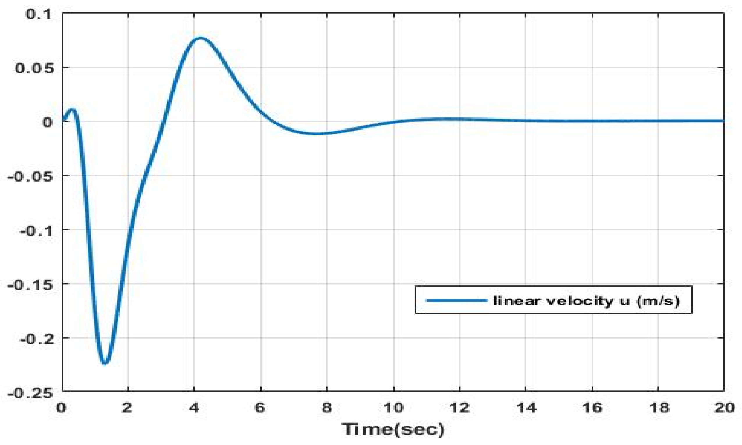
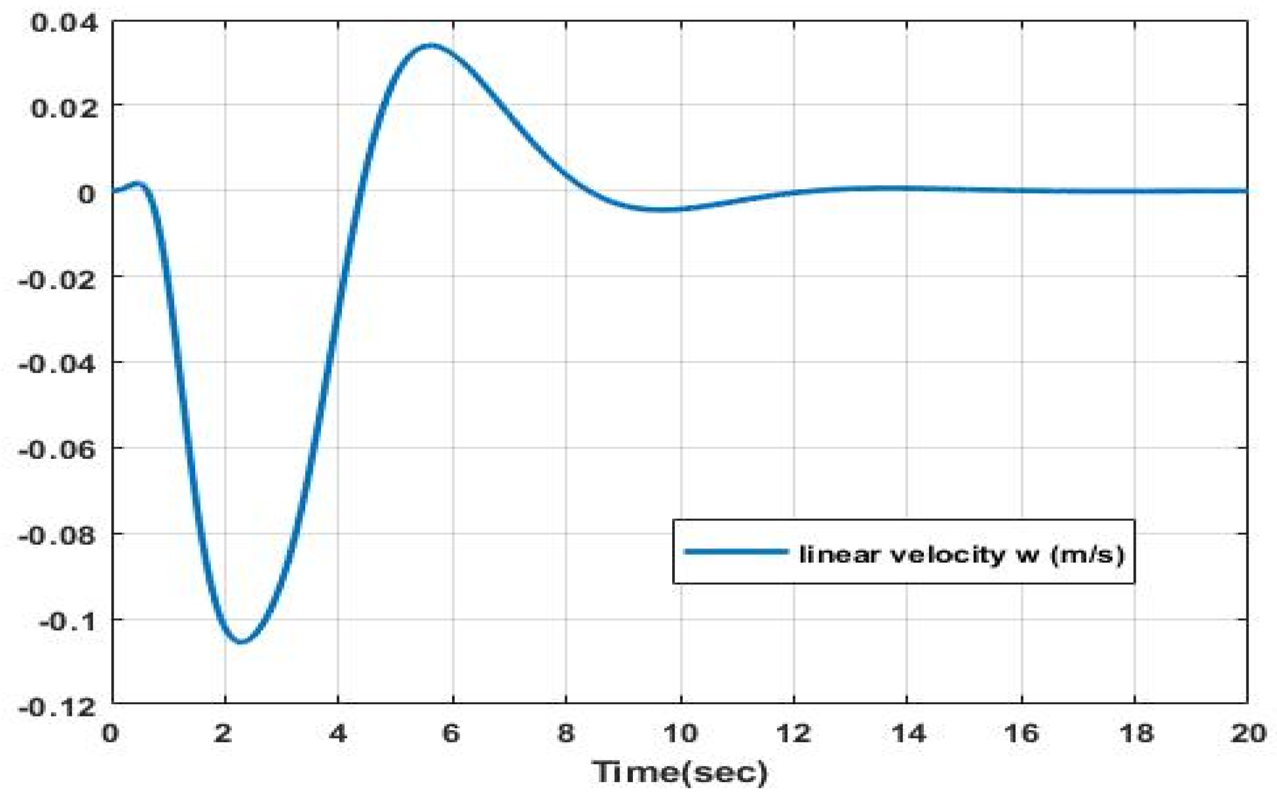
Numerical simulations were carried out using a MATLAB R2019a-based implementation to assess the practical effectiveness of the proposed control strategy. To illustrate the stabilization capability of the designed controller, we considered a representative maneuver involving the XSF quadrotor operating near its nominal equilibrium configuration. This scenario simulates a disturbance induced by a wind gust, modeled as a perturbation of approximately π/6 radians simultaneously in both pitch and roll axes.

The simulation results serve to evaluate the dynamic response of the system under sudden attitude deviations and demonstrate the robustness of the proposed quasi-LPV control scheme in restoring the system to its desired stable state.

Below is the useful inertial data from the XSF.

Mass m = 2.5 kg; gravity g = 10 ms⁻².

Inerties: I_xx = 224,931.10⁻⁷ kg.m²; I_yy = 222,611.10⁻⁷ kg.m²; I_zz = 325,130.10⁻⁷ kg.m².

Constants: I_R = 100.10⁻⁷ kg.m²; K_M = 9.10⁻⁶; K_T = 10⁻⁵.

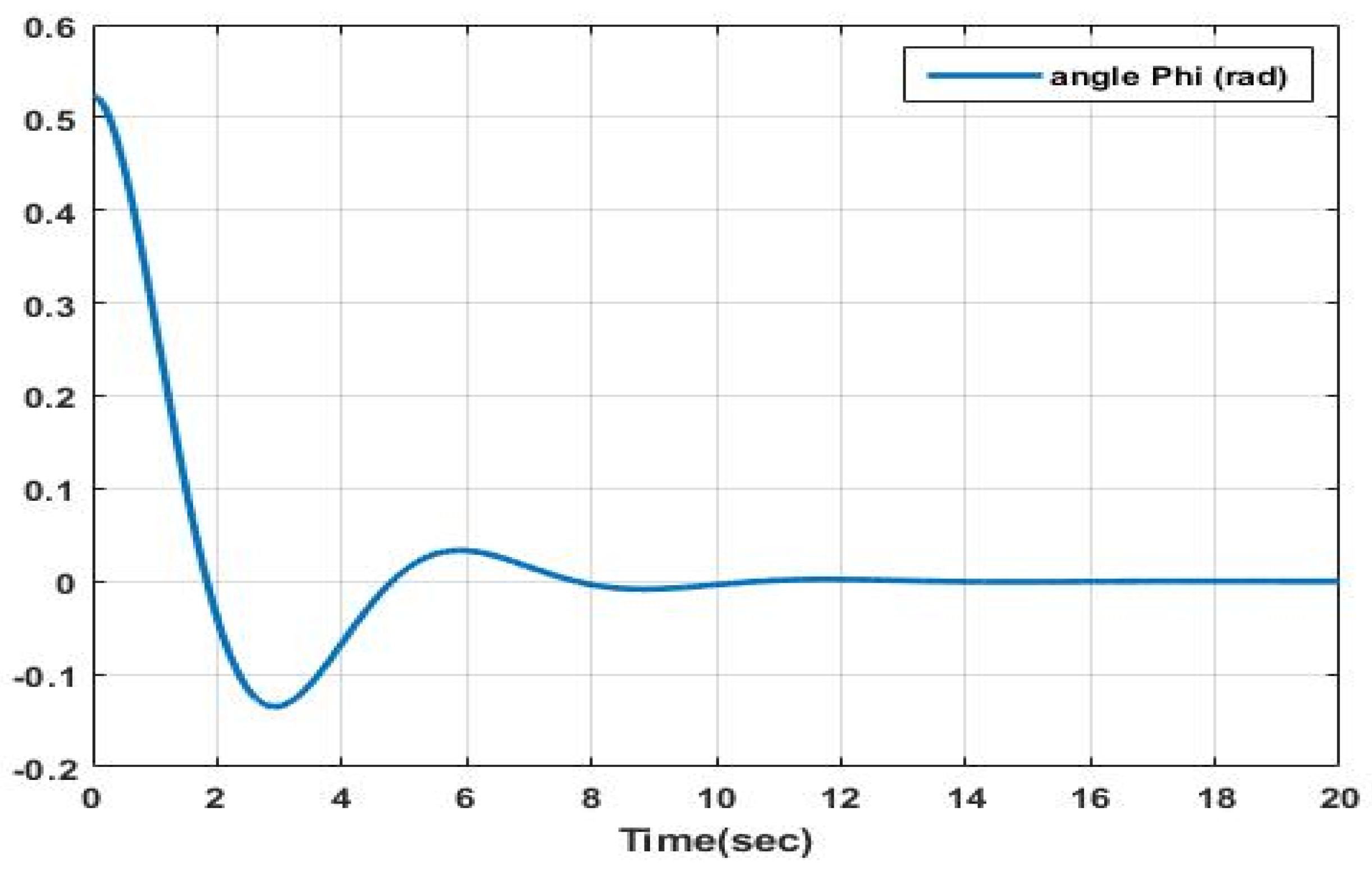
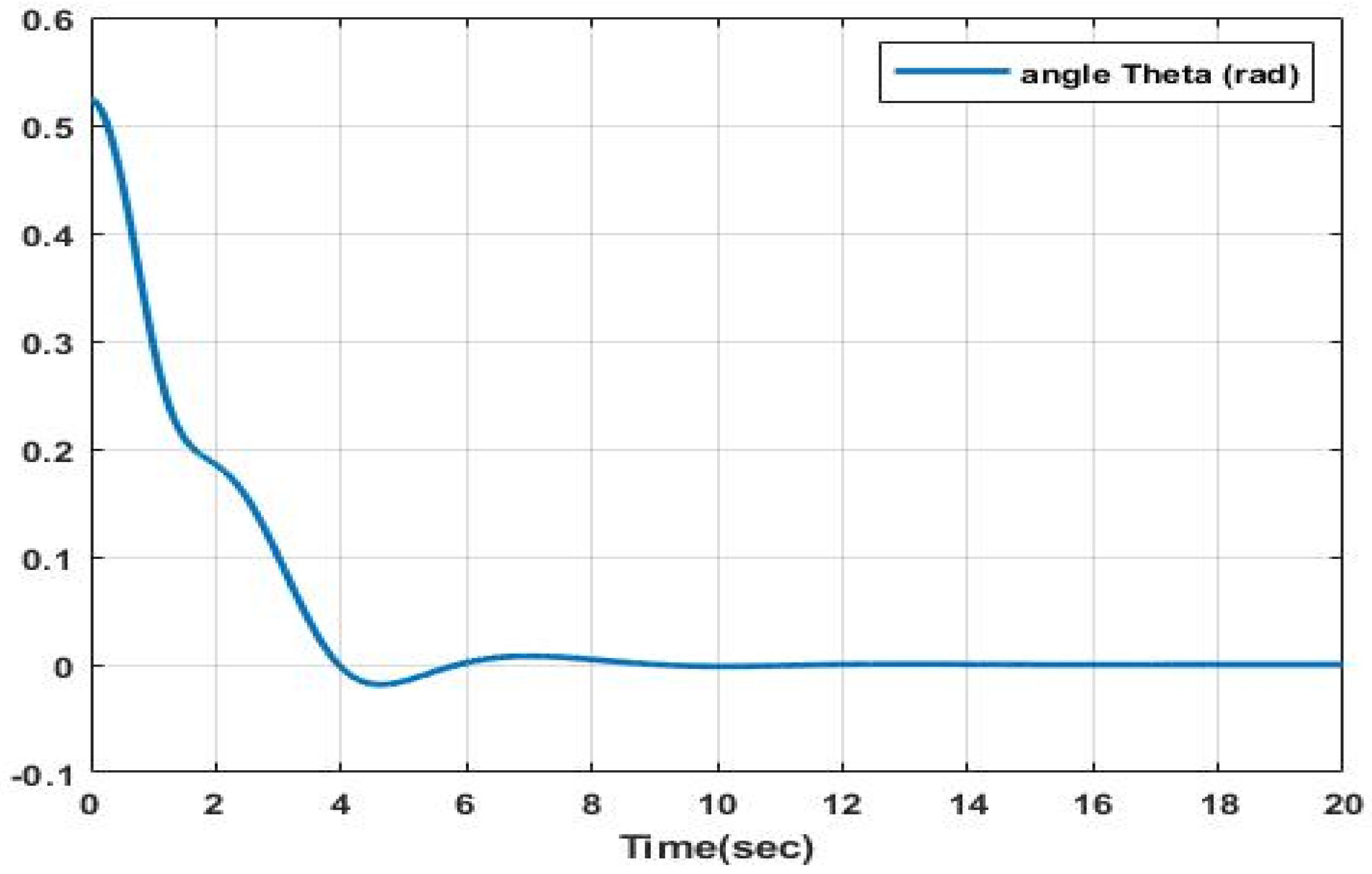
As evident from Figure 3, Figure 4, Figure 5 and Figure 6, the depictions illustrate the stabilization of both roll and pitch angles along with their derivatives. Additionally, they exhibit the prompt convergence of the linear velocities u, v, and w over a concise temporal interval. These observations collectively attest to the effectiveness of the q-LPV approach.

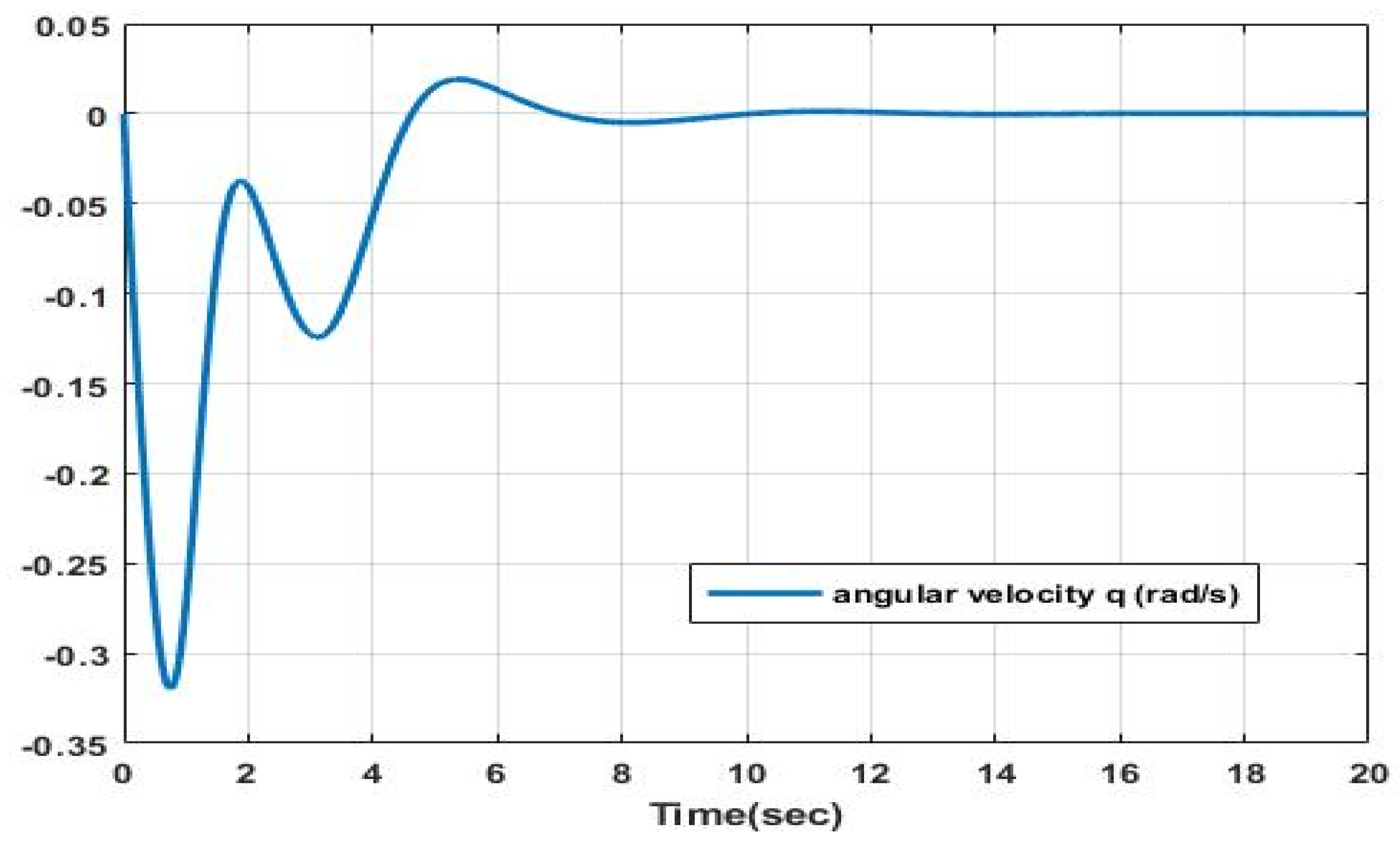
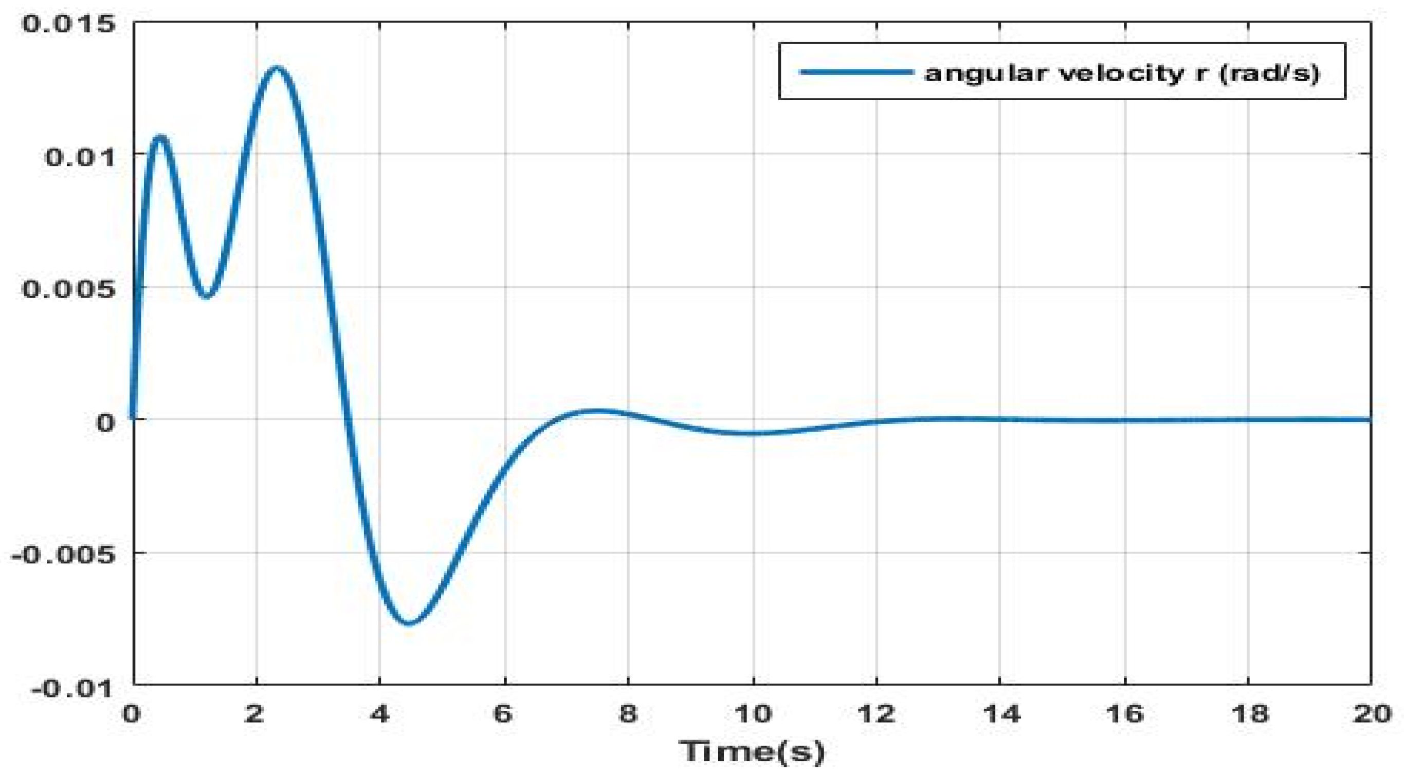
Figure 7, Figure 8 and Figure 9 provide substantiating evidence demonstrating that the implemented control law facilitates effective convergence and stabilization of the angular velocities p, q, and r.

On the other hand, Figure 10 shows the proper stabilization of the drone in the x and z positions.

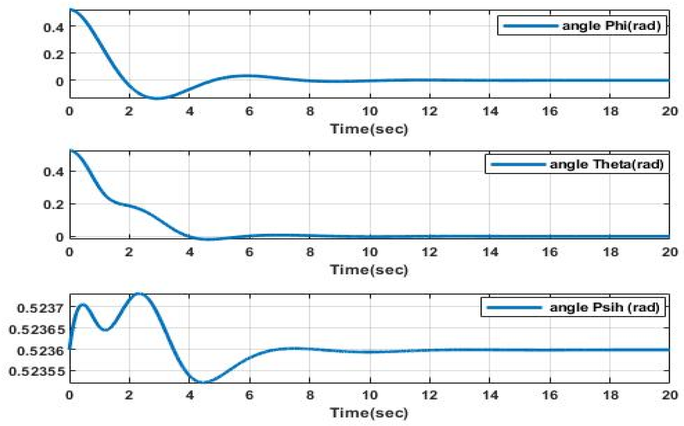
Figure 11, on the other hand, presents the time-based changes in the XSF’s orientation, highlighting minimal deviations and fast convergence toward a stable state.

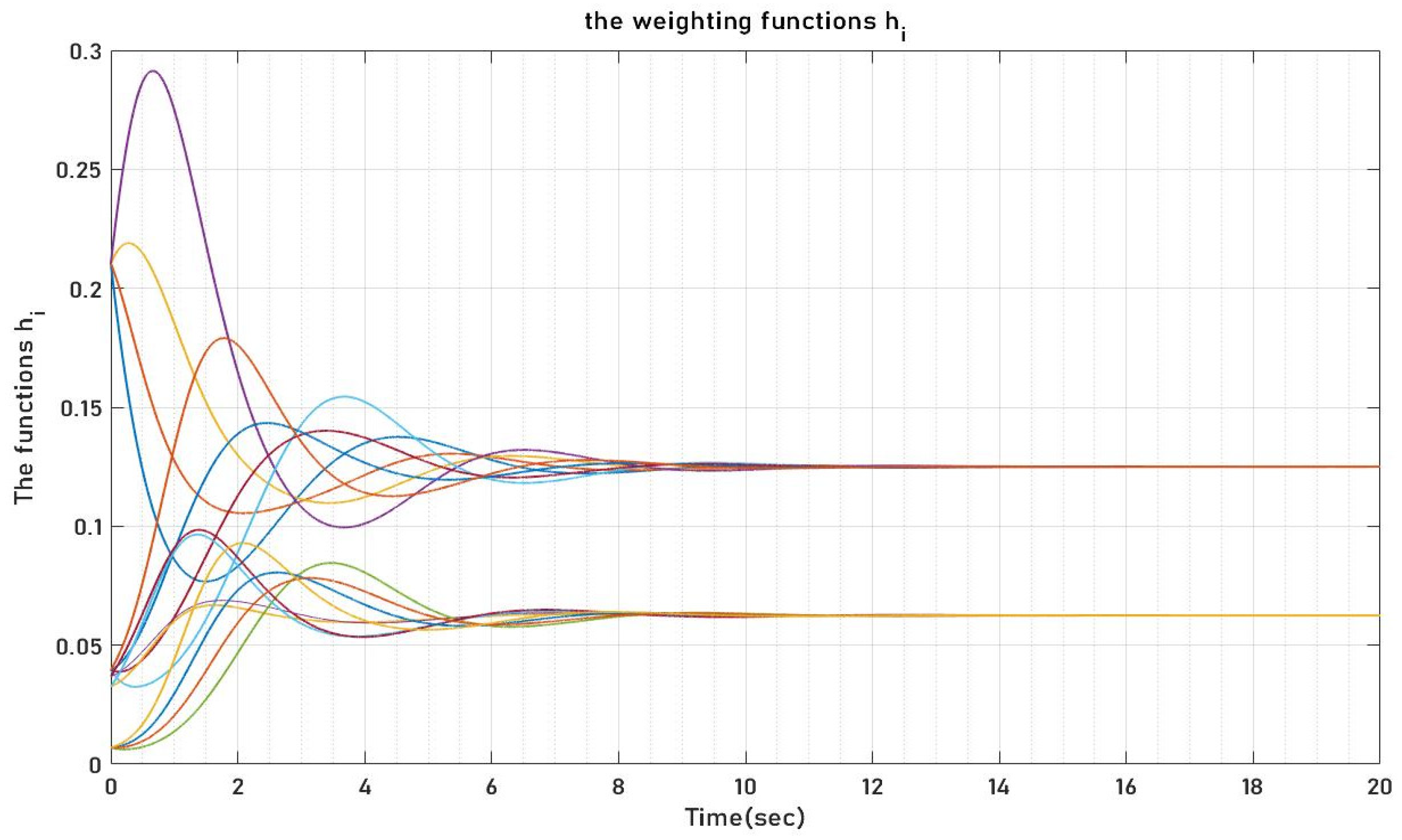
The graphical representation in Figure 12 distinctly reveals that the weighting functions h_i reside consistently within the range of 0 and 1. This observation underscores the convex nature of the polytope selected by the q-LPV strategy. The behavior of the different weighting functions h_i is shown below in Figure 12.

6. Comparison with Reference Results

To clearly demonstrate the performance and effectiveness of the quasi-LPV approach, it must be applied to other types of quadrotors; for example, we take the model of Torres et al. [24], and this type of quadrotor is modeled by the following system [24]:

$$\left\{\begin{array}{l}\ddot{\phi }={\displaystyle \frac{1}{I_x}}\left[\left(I_y-I_z\right)\dot{\theta }\dot{\psi }-k_{fax}{\dot{\varphi }}^2-J_r\dot{\theta }\overline{W}+l{U}_2\right]\\ \ddot{\theta }={\displaystyle \frac{1}{I_y}}\left[\left(I_z-I_x\right)\dot{\psi }\dot{\varphi }-k_{fay}{\dot{\theta }}^2+J_r\dot{\varphi }\overline{W}+l{U}_3\right]\\ \ddot{\psi }={\displaystyle \frac{1}{I_z}}\left[\left(I_x-I_y\right)\dot{\theta }\dot{\varphi }-k_{faz}{\dot{\psi }}^2+l{U}_4\right]\end{array}\right.$$

(33)

We can choose the state vector for the dynamic model of this quadrotor $X={[\varphi ,\theta ,\psi ,\dot{\varphi },\dot{\theta },\dot{\psi }]}^T$ and the control vector $U={[{\omega }_1,{\omega }_2,{\omega }_3,{\omega }_4,{{\omega }^2}_1,{{\omega }^2}_2,{{\omega }^2}_3,{{\omega }^2}_4]}^T$ such that: $\dot{X}=AX+BU$.

Now applying the quasi-LPV approach and taking as non-linear points the following variables:

$$\left\{\begin{array}{l}{z}_1=\dot{\varphi }\\ z_2=\dot{\theta }\\ z_3=\dot{\psi }\end{array}\right.\mathrm{These}\mathrm{points}\mathrm{are}\mathrm{bounded}\left\{\begin{array}{l}{z}_1^{\min }\le z_1\le z_1^{\max }\\ z_2^{\min }\le z_2\le z_2^{\max }\\ z_3^{\min }\le z_3\le z_3^{\max }\end{array}\right.$$

Then, the structural configuration of quasi-LPV is delineated as follows:

$$\begin{gathered} \dot{X}={\displaystyle \sum _{i=1}^8{h}_i(X)\left[A_{i}X+B_{i}U\right]}=A_{i}X+B_{i}U \\ \mathrm{with} \\ {A}_i=\left(\begin{array}{cccccc}0& 0& 0& 1& 0& 0\\ 0& 0& 0& 0& 1& 0\\ 0& 0& 0& 0& 0& 1\\ 0& 0& 0& {\displaystyle \frac{k_{fax}}{I_x}}\dot{\varphi }& 0& {\displaystyle \frac{I_y-I_z}{I_x}}\dot{\theta }\\ 0& 0& 0& 0& {\displaystyle \frac{k_{fay}}{I_y}}\dot{\theta }& {\displaystyle \frac{I_z-I_x}{I_y}}\dot{\varphi }\\ 0& 0& 0& {\displaystyle \frac{I_x-I_y}{I_z}}\dot{\theta }& 0& {\displaystyle \frac{k_{faz}}{I_z}}\dot{\psi }\end{array}\right);B=\left(\begin{array}{cccccccc}0& 0& 0& 0& 0& 0& 0& 0\\ 0& 0& 0& 0& 0& 0& 0& 0\\ 0& 0& 0& 0& 0& 0& 0& 0\\ {\displaystyle \frac{J_r}{I_x}}\dot{\theta }& -{\displaystyle \frac{J_r}{I_x}}\dot{\theta }& {\displaystyle \frac{J_r}{I_x}}\dot{\theta }& -{\displaystyle \frac{J_r}{I_x}}\dot{\theta }& -{\displaystyle \frac{l{k}_t}{I_x}}& 0& {\displaystyle \frac{l{k}_t}{I_x}}& 0\\ -{\displaystyle \frac{J_r}{I_y}}\dot{\varphi }& {\displaystyle \frac{J_r}{I_y}}\dot{\varphi }& -{\displaystyle \frac{J_r}{I_y}}\dot{\varphi }& {\displaystyle \frac{J_r}{I_y}}\dot{\varphi }& 0& -{\displaystyle \frac{l{k}_t}{I_y}}& 0& {\displaystyle \frac{l{k}_t}{I_y}}\\ 0& 0& 0& 0& {\displaystyle \frac{l{K}_d}{I_z}}& -{\displaystyle \frac{l{K}_d}{I_z}}& {\displaystyle \frac{l{K}_d}{I_z}}& -{\displaystyle \frac{l{K}_d}{I_z}}\end{array}\right) \end{gathered}$$

(34)

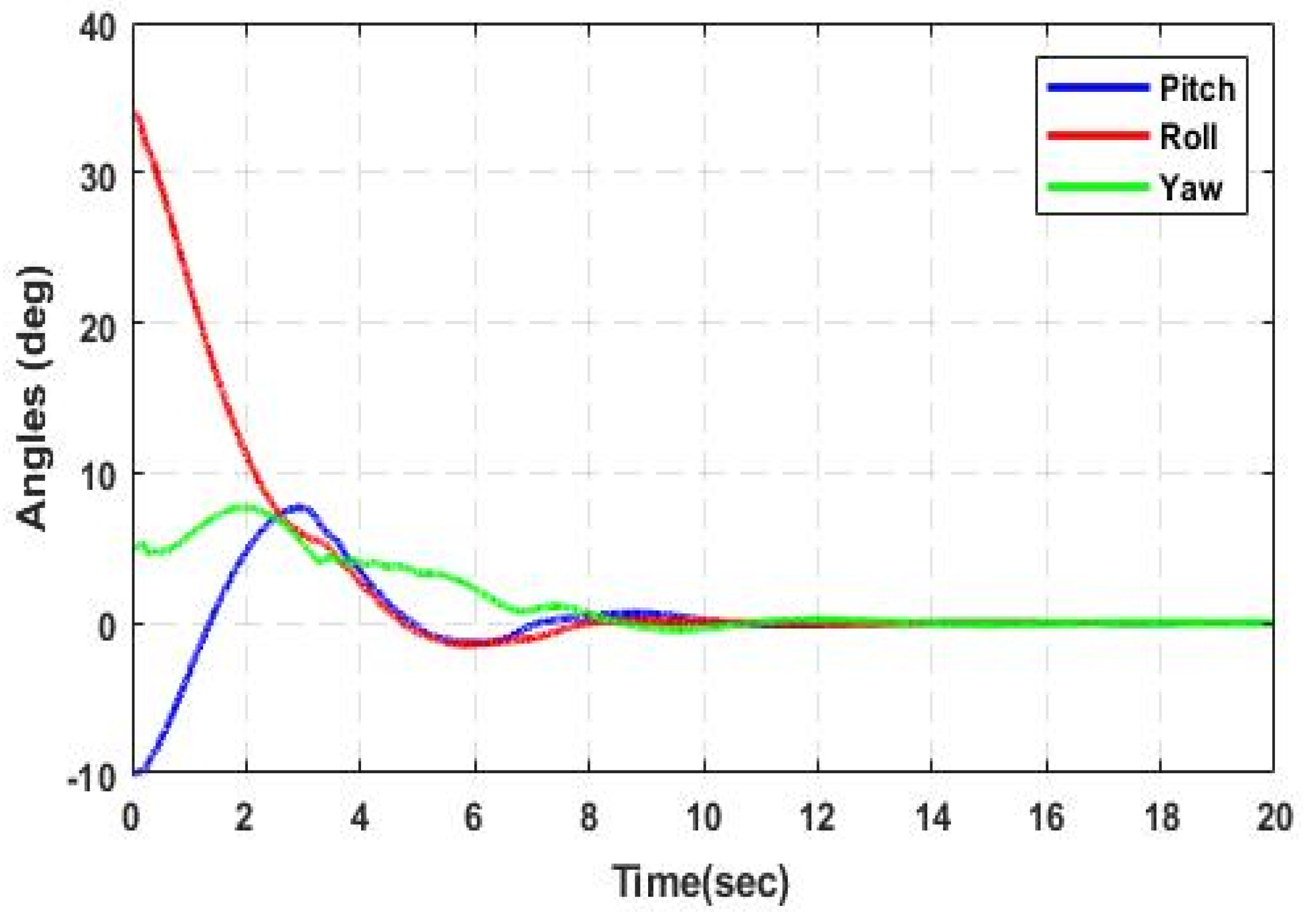
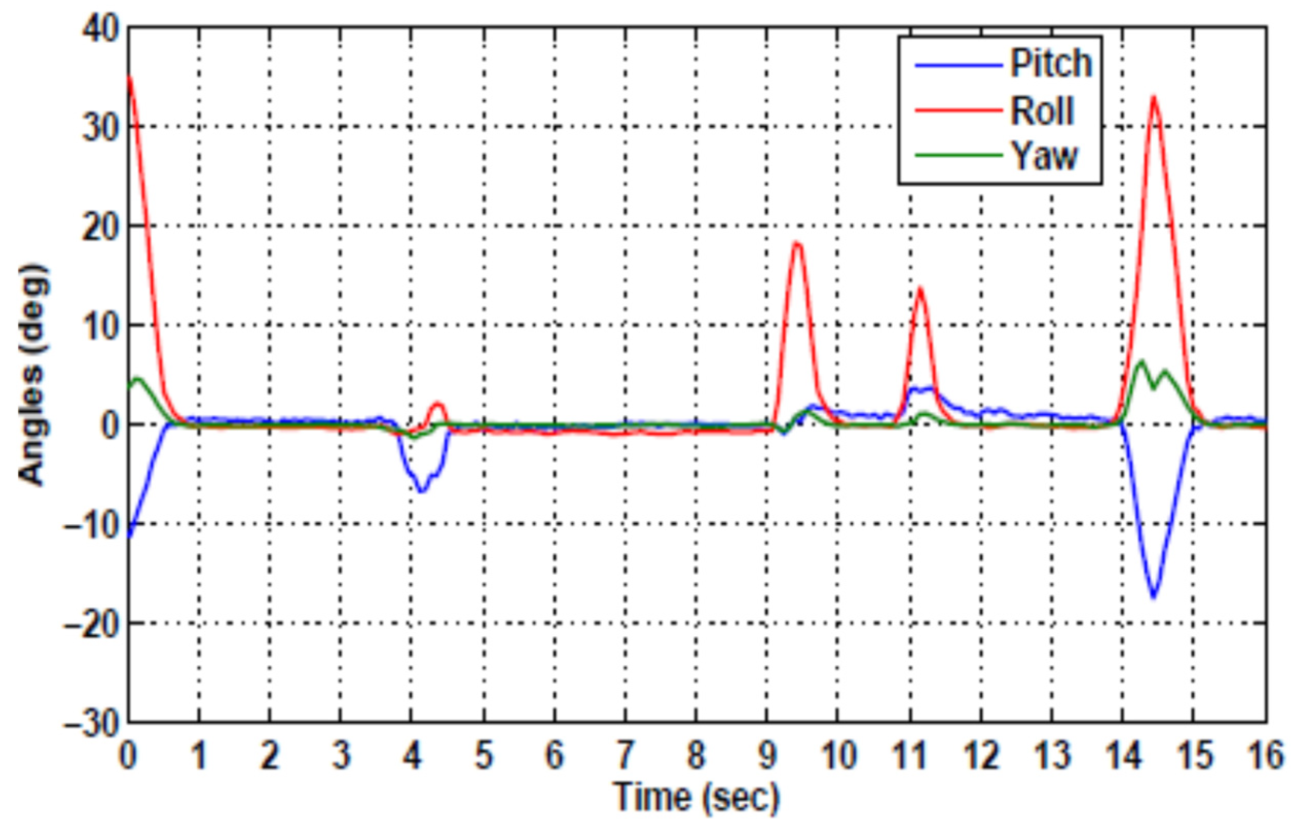
As illustrated in the comparative Figure 13 and Figure 14, the q-LPV (quasi-linear parameter-varying) control approach employed in our study exhibits a longer transient response time in stabilizing the quadrotor when compared to the performance reported by Torres et al. Although the initial stabilization phase is relatively slower, this behavior is an inherent consequence of the conservative design characteristics associated with polytopic control strategies. Nonetheless, the q-LPV method demonstrates a significant advantage in terms of robustness and sustained performance. Owing to its polytopic structure, which effectively captures the system’s dynamic variations across a defined parameter space, the proposed controller ensures persistent stability of the vehicle over time. This enables the quadrotor not only to reach but also to maintain a steady equilibrium state in the vicinity of the designated target position, thereby enhancing its suitability for missions requiring prolonged hovering or precise station-keeping capabilities.

7. Conclusions

This study began with the formulation of a comprehensive dynamic model for an X-shaped six-rotor flying (XSF) drone, incorporating the non-linear and coupled dynamics characteristic of such aerial vehicles. The central outcome of the work was the successful stabilization of the drone at a designated equilibrium point, confirming the effectiveness of the proposed control design. The primary focus was placed on developing a structured methodology for designing controllers tailored to non-linear systems influenced by time-varying and potentially unstructured external disturbances, all represented through a quasi-linear parameter-varying (Quasi-LPV) framework.

A major theoretical contribution of the paper lies in the derivation of sufficient stability conditions, cast in terms of linear matrix inequalities (LMIs), which guarantee robust performance across the entire parameter space of the polytopic system. These LMIs offer a convex and computationally tractable means to synthesize state feedback controllers capable of addressing the challenges posed by non-linearities and dynamic uncertainties within the system.

The effectiveness of the proposed method was validated through a set of numerical simulations, which confirmed reliable stabilization under realistic disturbance scenarios. Furthermore, a comparative assessment with an existing reference approach—focused on quadrotor stabilization—demonstrated the competitiveness and robustness of our control strategy, particularly in terms of its long-term stability and adaptability to parameter variations.

Future Work:

Several avenues remain open for further investigation. The first perspective concerns the generalization of this technique to trajectory tracking studies. Secondly, the extension of the proposed Quasi-LPV control methodology to accommodate actuator constraints and saturation effects would enhance its practical applicability. Thirdly, integrating online parameter estimation or adaptive gain scheduling mechanisms could allow the controller to dynamically adjust to changes in the drone’s operating conditions, thereby improving responsiveness and robustness. Additionally, experimental validation on a physical XSF drone platform is essential to confirm the real-world feasibility of the method. Finally, exploring decentralized or distributed control architectures for coordinated flight in multi-agent drone systems based on the Quasi-LPV formalism represents a promising direction for advancing autonomous aerial swarm technologies.