Stochastic Blade Pitch Angle Analysis of Controllable Pitch Propeller Based on Deep Neural Networks

Abstract

The accuracy of the blade pitch angle (BPA) motion in controllable pitch propellers (CPPs) is considered crucial for the efficacy and reliability of marine propulsion systems. The pitch adjustment process of CPPs is highly complex and influenced by various uncertain factors. A parametric kinematic model for the pitch adjustment process for CPPs was established, incorporating the geometric dimensions and material surface friction coefficients caused during workpiece production as uncertainty parameters. The aim was to establish the correspondence between these uncertainty parameters and the BPA of CPPs. A large dataset was generated by batch calling on Adams. Based on the collected dataset, five surrogate models (e.g., deep neural network (DNN), Kriging, support vector regression (SVR), random forest (RF), and polynomial chaos expansion Kriging (PCK)) were constructed to predict the BPA. Among these, the DNN approach demonstrated the highest prediction accuracy. Accordingly, the influence of uncertainties on the BPA was investigated using the DNN model, focusing on variations in the slider width, crank pin diameter, crank disc diameter, piston rod–slider friction coefficient, crank pin–slider friction coefficient, and hub bearing–crank disc friction coefficient. The high-fidelity model established in this study can replace the kinematic model of the CPP pitch adjustment process, significantly improving computational efficiency. The research findings also provide important references for the design optimization of CPPs.

1. Introduction

A controllable pitch propeller (CPP) is a maritime propulsion apparatus that facilitates blade rotation and pitch modification using an actuation mechanism incorporated into the hub assembly [1]. CPP systems dynamically adjust the blade pitch angle (BPA) under different conditions to maximize the prime mover power output and improve the propeller efficiency in off-design operational states [2]. Notably, CPPs stand out for their ability to reverse thrust without engine direction alteration. This capability boosts a ship’s maneuverability and quickness [3]. These advanced propulsors have gained widespread adoption in marine vessels requiring multi-mode operations and enhanced maneuverability, including tugboats, oceangoing fishing vessels, and icebreakers [4]. Systematic deviations between the theoretical and actual BPA often indicate kinematic parameter degradation and contact pair stiction effects caused by long-term wear at critical motion interfaces (e.g., piston rod–slider, crank pin–slider, and hub bearing–crank disc assemblies). When such cumulative deviations reach critical thresholds, they signal the requirement for maintenance cycle inspections or component replacements in CPP systems. Consequently, developing adaptive BPA prediction models based on critical component wear states holds significant engineering value for ensuring marine propulsion system reliability.

Through the development of a virtual prototype model for CPPs, Xie et al. [5] conducted dynamic simulations to comparatively analyze the force transmission characteristics and kinematic responses of pitch adjustment mechanism components under both frictional and friction-free conditions. Their study quantitatively evaluated hydraulic pressure requirements throughout the complete pitch adjustment cycle. Yan [6] conducted a kinematic analysis of the slider mechanism in CPPs, determining the motion parameters of individual components within the pitch adjustment mechanism under specified operational conditions. By systematically comparing the experimentally derived motion parameters with theoretical design values, this study established a critical theoretical foundation for optimizing the design and manufacturing processes of CPP pitch adjustment mechanisms. Dang et al. [7] designed an amphibious propeller for multi-rotor hybrid aquatic–aerial vehicles (HAAVs) utilizing a design optimization framework based on a deep neural network surrogate model and particle swarm optimization. Gebauer et al. [8] designed controllers for variable pitch propeller propulsion drives (VPPPDs) utilizing the pitch control algorithm (PCA) and adaptive pitch control algorithm (APCA) based on the knowledge of propeller and brushless motor properties.

However, scholarly investigations of CPP have predominantly focused on kinematic simulations and control optimization of pitch adjustment mechanisms. A critical research gap persists in systematically analyzing the motion characteristics under multi-joint clearance conditions and in developing efficient reliability assessment methodologies for propulsion functionality. Notably, clearance-induced deviations in key kinematic pairs—including piston rod–slider, crank pin–slider, and hub bearing–crank disc assemblies—generate discrepancies between actual pitch angles and feedback signals. When such deviations exceed critical thresholds, they compromise pitch adjustment accuracy, potentially destabilizing vessel navigation [9]. This functional gap necessitates a hybrid uncertainty analysis framework combining qualitative failure mode assessment with quantitative probabilistic modeling to evaluate the mechanism’s capability in executing specified operational functions.

In the past decade, machine learning and data-driven surrogate modeling have revolutionized computational mechanics through their unparalleled capacity to decode high-dimensional nonlinear interactions [10,11,12,13,14,15,16,17,18]. These methodologies excel in establishing input–output correlations that traditional physics-based models often struggle to quantify, particularly when addressing systems with coupled uncertainties [19]. Scholars initially used RF [20] and SVR [21,22] to study model uncertainty, achieving good predictive performance. Within marine propulsion engineering, mechanical systems, like CPPs, exhibit inherent nonlinear dynamics arising from multi-clearance couplings and transient friction effects—a complexity that conventional multibody dynamics simulations frequently oversimplify. Tahir et al. [23] predicted the buckling load of thin cylindrical shells under axial compression utilizing an artificial neural network (ANN) trained with experimental data. A non-intrusive Kriging-based reduced-order model [24] was developed to predict the brittle fracture propagation in quasi-static and dynamic regimes.

Traditional approaches can evaluate CPP motion, but they are computationally slow and struggle with complex concerns, like part clearances and friction variations. This work used DNN, PCK, and RF models to quickly estimate how critical aspects, like part size mistakes and friction coefficients, affect BPA. For the first time, we evaluated the combined effect of random fluctuations in six crucial parameters (slider width, crank pin diameter, crank disc diameter, and three friction coefficients) on the blade angle by extensive data simulations. Studies have revealed that the DNN model accurately analyzes real-world performance changes due to, by part, better wear than SVR and Kriging. This method speeds up CPP design optimization and reliability testing, especially for manufacturing defects and long-term wear.

2. Kinematic Simulation Analysis

In the CPP model, the BPA was adjusted through an internal mechanism within the hub, which rotates the blades to alter their geometric orientation. This dynamic adjustment enables the propeller to achieve optimal pitch regulation and to adapt to various operating conditions, thereby enhancing reverse thrust, acceleration, and braking performance. The blade actuation system employs a crank mechanism, where the linear reciprocating motion of the piston rod is converted into rotational motion of the blade section via a slider. Specifically, the sliding block translates the axial movement of the piston rod into an angular displacement of the crank disc through the engagement between the crank pin and the slider. However, during the pitch adjustment process, the operational reliability of this mechanism is significantly influenced by the mechanical clearances and friction coefficients at three critical interfaces: (1) the piston rod–slider interface, (2) the crank pin–slider interface, and (3) the crank disc–hub bearing interface. Variations in these geometric clearances and tribological properties can lead to operational inefficiencies, misalignment issues, and to the potential failure of the pitch control system under transient loading conditions.

The 1/5 scaled geometric model of a marine controllable pitch propeller was constructed in SolidWorks 2021, as shown in Figure 1, comprising the hub casing, crank disk, piston rod assembly, and slider transmission mechanism. A dynamic model was established in Adams based on the topological relationships among hub components. The kinematic constraints included the rotational drive of the hub assembly about the central axis (propeller RPM-based) and a zero-displacement translational constraint on the piston rod–hub sliding pair to immobilize axial movement.

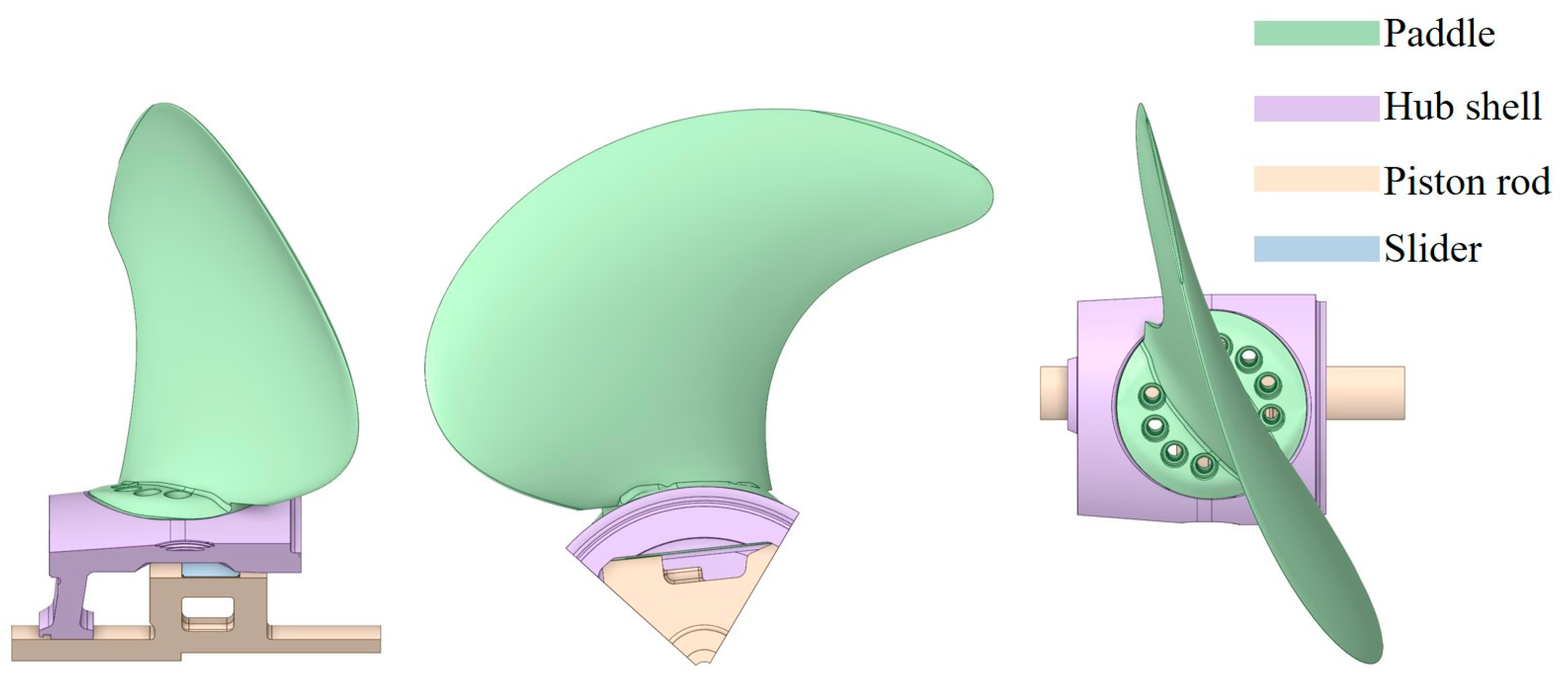
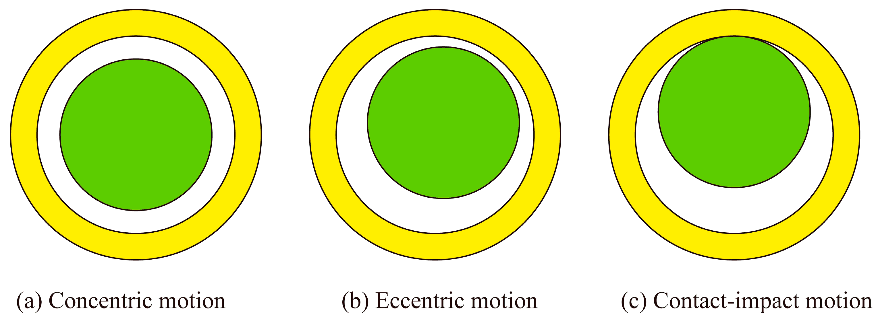
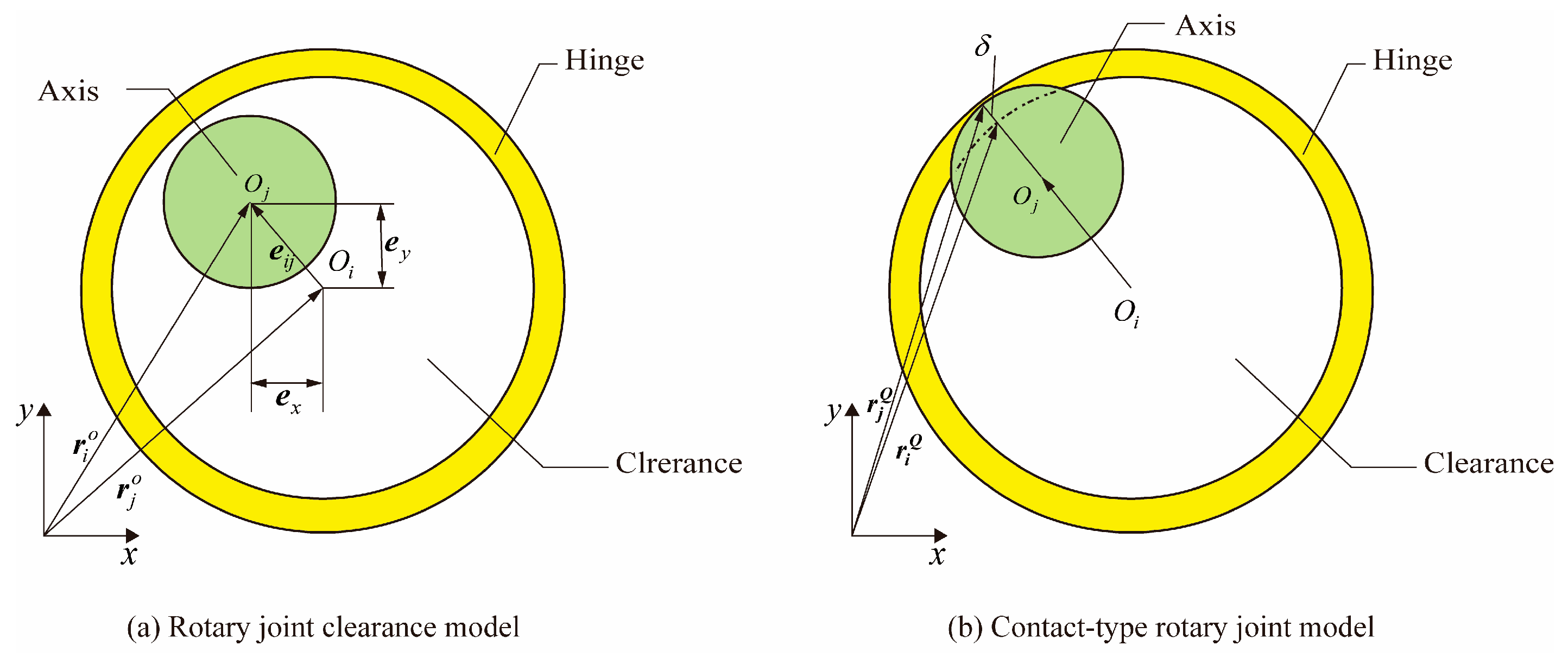
2.1. Rotary Clearance Joint Model

The wear generated by the slider–crank pin and hub bearing–crank disc during motion was simulated using the Rotary Clearance Joint Mode. This model simplifies the hinged portion into a rotational clearance joint model. The model was constructed based on a local floating Cartesian coordinate system, with the rotation axis center as the origin and the clearance vector pointing to the potential contact area between the hinge and the shaft center. Its value range is limited by the radius tolerance of the hinge and the axis, reflecting both manufacturing errors and the contact state of the kinematic pair elements, thus effectively reproducing the dynamic interaction between components.

The crank pin rotates within the slider, driving the propeller blade connected via blade root bolts. Due to the clearance between the crank pin and slider, three motion patterns may occur in the slider bearing, as shown in Figure 2. Simultaneously, the crank disk rotates within the propeller hub bearing, where the hub bearing–crank disk clearance constrains the crank disk’s operational envelope, causing deviations in BPA. The kinematic interactions between the hub bearing and crank disk also exhibit three corresponding states: concentric motion, eccentric motion, and contact–impact motion.

As shown in Figure 3, $O_i$ and $O_j$ represent the centers of the hinge and axis, respectively; while ${\mathit{r}}_i^o$ and ${\mathit{r}}_j^o$ denote the specific position vectors of the hinge and axis in the global coordinate system, respectively. The vector representation of the clearance is as follows:

$${\mathit{e}}_{\mathit{i}\mathit{j}}={\mathit{r}}_{\mathit{i}}^{\mathit{o}}-{\mathit{r}}_{\mathit{j}}^{\mathit{o}}.$$

(1)

The eccentricity of the clearance vector can be defined as follows:

$${\mathit{e}}_{\mathit{ij}}=\sqrt{{\mathit{e}}_{\mathit{x}}^{\mathbf{2}}+{\mathit{e}}_{\mathit{y}}^{\mathbf{2}}}.$$

(2)

The deformation $\delta$ caused by impact can be defined as follows:

$$\delta ={\mathit{e}}_{\mathit{ij}}-C.$$

(3)

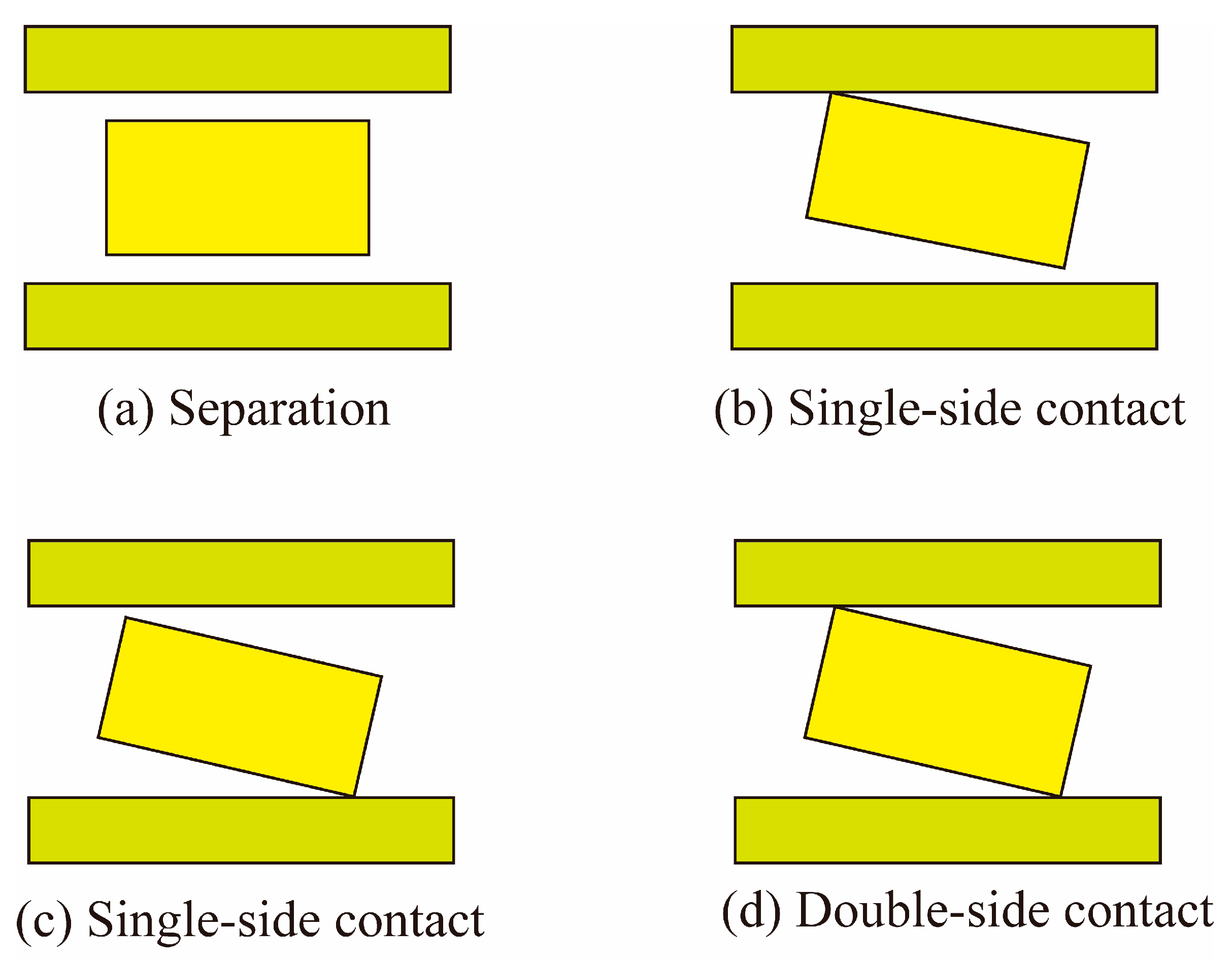
2.2. Contact Force Model

This study established a nonlinear equivalent spring-damping model to simulate the contact behavior between the hinge and the axis. By introducing nonlinear stiffness and damping coefficients, this model overcomes the limitations of traditional linear models, accurately depicting dynamic phenomena, such as collisions and impacts during the motion of systems with clearance. It effectively achieves the dynamic simulation of clearance mechanisms. This model can be expressed as follows:

$$F_n=F_k+F_d=K{\delta }^m+C(\delta )\dot{\delta },$$

(4)

where $F_n$ represents the normal contact force, $K$ represents the stiffness coefficient, $\delta$ represents the penetration depth, $m$ is an exponential term, $C(\delta )$ represents the damping coefficient related to $\delta$, and $\stackrel{·}{\delta }$ represents the relative velocity.

The elastic restoring force $F_k$ is determined by the Hertz contact theory:

$$F_k=K{\delta }^{1.5}.$$

(5)

To address the shortcomings of the linear damping model and meet the boundary conditions of the contact interface, a non-linear damping model was adopted. This model can more accurately describe the damping force, and it is used to precisely define the damping force $F_d$.

$$F_d=D\stackrel{·}{\delta },$$

(6)

$$C={\displaystyle \frac{0.75(1-e^2)K{\delta }^{3/2}}{V_0}},$$

(7)

where $C$ is the damping coefficient that is related to the coefficient of restitution and the contact stiffness, $e$ is the restitution coefficient, and $V_0$ is the initial velocity of the contact point.

The pitch adjustments capability of the CPP was realized by the synchronized interaction of its components. Clearance fit configurations were utilized between the slider and piston rod, the crank pin and slider, and the propeller hub bearing and crank disc, as depicted in Figure 4. The clearance dimensions between the components were affected by initial machining and assembly faults and were dynamically increased by frictional wear during operation.

Table 1. The clearance fit dimensions between components.

Number	Component	Initial Range of Clearance/mm
Clearance I	Piston Rod	[0.025, 0.075]
	Slider
Clearance II	crank pin	[0.015, 0.100]
	Slider
Clearance III	Hub Bearing	[0.160, 0.320]
	Crank Disc

enumerates the clearance fit dimensions among the various components, with the size ranges based on the allowable machining tolerances of the respective parts.

During pitch adjustment, the piston moves under differential oil pressure from both chambers, driving the piston rod displacement. This motion propels the slider within the piston rod slideway, thereby inducing crank pin rotation. The kinematic state of the slider critically governs BPA accuracy. Due to the clearance between the piston rod and slider, four distinct motion patterns may occur within the slideway, as shown in Figure 5.

2.3. Friction Model

In this study, the modified Coulomb friction model was selected due to its simplicity and effectiveness. This model is sufficient for handling most calculation scenarios and avoids the additional state—variables required by more complex models. The friction model chosen in this study can be expressed as follows:

$$F_T=-c_f{c}_d{F}_N{\displaystyle \frac{V_t}{\left|\left|V_t\right|\right|}},$$

(8)

where $c_f$ is the friction coefficient, and $V_t$ is the relative tangential velocity. In addition, the dynamic correction coefficient $c_d$ is given by the following formula:

$$c_d=\left\{\begin{array}{ccc}0& & ‖V_t‖\le V_0\\ {\displaystyle \frac{‖V_t‖-V_0}{V_1-V_0}}& & V_0\le ‖V_t‖\le V_1\\ 1& & ‖V_t‖\ge V_1\end{array}\right..$$

(9)

In the formula, $V_0$ and $V_1$ are the specified tolerances of the tangential velocity, and the parameters were obtained according to the research in the literature. The dynamic correction—factor $c_d$—can prevent the change in the friction–force direction when the tangential velocity is almost zero.

To analyze the influence patterns of the different clearance positions and sizes on the dynamic characteristics of components, a contact collision simulation model with clearance between two components was established. The contact between the slider and the piston rod groove was surface-to-surface contact; therefore, dummy objects were created on both sides of the slider and fixedly connected to the groove, thereby, respectively, establishing contact relationships with the slider.

Table 2. The parameters of contact and collision between the slider and the dummy body.

Model Parameters	Symbol	Value
Slider width (mm)	$L$	230
Stiffness coefficient (N/m)	$K$	$1.0\times {10}^5$
Damping coefficient (N·(s/m))	$D$	10.0
Restitution coefficient	$e$	2.2
Coefficient of maximum static friction	${\mu }_s$	0.3
Coefficient of kinetic friction	${\mu }_d$	0.1

presents the parameters of the contact and collision model between the slider and dummy object.

This study analyzed BPA under two conditions (the results of which are shown in Figure 6): the ideal condition and the collision model. The BPA was less than the ideal condition because, at that moment, the slider primarily makes contact with the left dummy object.

The influence of mechanical clearances on the BPA dynamics was systematically investigated through parametric variation of the dummy objects’ geometries. Five distinct clearance configurations (0.025 mm, 0.050 mm, 0.075 mm, 0.100 mm, and 0.125 mm) were implemented at three critical interfaces. The results are shown in Figure 7.

This study employed parametric modeling in Adams to adjust the geometric dimensions of the slider, crank disk, and crank pin. Through batch processing of Adams calculation files using MATLAB 2020R1, the .cmd files were iteratively invoked to systematically acquire data characterizing the correspondence between the BPA and input variables.

3. Methodology

3.1. Deep Neural Networks

The DNN model constructed in this study includes an input layer with six key parameters, an output layer that determines the BPA, and multiple hidden layers. Each hidden layer in the DNN model consists of numerous neurons. The number of neurons in the hidden and output layers, weights, biases, and activation functions collectively define the nonlinear relationship between the uncertainty parameters and the output blade rotation angle. The mathematical representation of a single neuron is as follows:

$$y_j^{(k)}=f\left(b^{k-1}+{\displaystyle \sum _{i=1}^{m^{k-1}}{w}_{i,j}^{(k)}}{y}_i^{(k-1)}\right),$$

(10)

where $y_j^{(k)}$ denotes the result of the $j^{th}$ neuron in the $k^{th}$ layer, $m^{k-1}$ represents the number of neurons in the previous layer, $w_{i,j}^{(k)}$ signifies the weight connecting to the $i^{th}$ neuron of the previous layer, and $b^{k-1}$ indicates the bias of the previous layer. In this study, Rectified Linear Unit (ReLU) was employed as the activation function due to its high computational efficiency and robust performance in mitigating issues of gradient vanishing or explosion, which is defined as follows:

$$f(x)=\left\{\begin{array}{l}0, x\le 0\\ x, x>0\end{array}\right..$$

(11)

The mean square error was used as the loss function, and it is defined as follows:

$$Loss={\displaystyle \frac{1}{n}}{\displaystyle \sum _{i=1}^n{({\widehat{y}}_i-y_i^{k_{out}})}^2},$$

(12)

where ${\widehat{y}}_i$ represents the predicted output value of the $i$-th by the DNN model, and $y_i^{k_{out}}$ represents the true label of the $i$-th sample. The DNN model used in this article consists of three hidden layers with 64, 32, and 16 neurons, respectively, as shown in Figure 8.

3.2. Other Surrogate Models

A CPP’s BPA is affected by various uncertain factors, exhibiting strong nonlinearity and randomness. SVR is a non-parametric machine learning algorithm based on statistical learning theory, as shown in Figure 9. Its core lies in mapping the original input space to a high-dimensional feature space using kernel functions, and it constructs an optimal hyperplane in this space to achieve a nonlinear mapping relationship between input variables and output responses with the goal of minimizing structural risk. Specifically, SVR can efficiently resolve the nonlinear coupling problem between the BPA and multiple uncertain factors by leveraging the nonlinear mapping capability of kernel functions. It can be expressed as follows:

$${\min }_{w,b,\xi ,{\xi }^{*}}{\displaystyle \frac{1}{2}}\Vert w{\Vert }^2+C{\displaystyle \sum _{i=1}^n({\xi }_i+{\xi }_i^{*})},$$

(13)

which is subject to

$$\left\{\begin{array}{c}{y}_i-w^T\varphi (x_i)-b\le ϵ+{\xi }_i\\ w^T\varphi (x_i)+b-y_i\le ϵ+{\xi }_i^{*}\\ {\xi }_i,{\xi }_i^{*}\ge 0\end{array}\right.,$$

(14)

where $w$ represents the weight vector, $b$ represents the bias term, $C$ is the regularization parameter used to balance the model’s complexity and fitting error, ${\xi }_i,{\xi }_i^{*}$ are slack variables allowing for a certain degree of error, $\varphi (x_i)$ is the function that maps input $x$ to a high-dimensional feature space, and threshold $ϵ$ is for insensitive loss, which does not calculate loss when prediction error is within [−ε, ε], and it is also a key parameter in controlling the ‘tolerable error range’ in SVR.

Kriging is widely used in constructing uncertainty surrogate models, with the core idea being to establish a stochastic process model through limited sample points. However, due to the uneven distribution of uncertain factors affecting BPA in the input space, and despite support for nonlinear kernel functions, Kriging’s modeling capability for extremely complex nonlinearities remains limited, which may significantly increase prediction errors. The Kriging model can be approximated as the sum of a random distribution function and a polynomial, and it is expressed as follows:

$$g_K(X)={\displaystyle \sum _{i=1}^p{f}_i}(X){\beta }_i+z(X),$$

(15)

where $g_K(X)$ represents the Kriging model to be solved, $f_i(X)$ is the basis function of the random vector $X$, ${\beta }_k$ is the coefficient of the trend function $f_i(X)$, and $z(X)$ is a stochastic process with local deviations having a mean of 0 and variance ${\sigma }^2$. Its covariance matrix components can be expressed as follows:

$$\mathit{Cov}\left[z\left({\mathit{x}}^{(i)}\right),z\left({\mathit{x}}^{(j)}\right)\right]={\sigma }^2\left[R\left({\mathit{x}}^{(i)},{\mathit{x}}^{(j)}\right)\right],$$

(16)

where $R\left({\mathit{x}}^{(i)},{\mathit{x}}^{(j)}\right)$ represents the correlation function of any two sample points.

According to Kriging theory, $g_K(\mathbf{X})$ follows a Gaussian distribution, and its ${\mu }_{g_K}$ and ${\sigma }_{g_K}^2$ can be expressed as follows:

$${\mu }_{g_K}(\mathit{x})={\mathit{f}}^{\mathrm{T}}(\mathit{x})\widehat{\mathit{\beta }}+{\mathit{r}}^{\mathit{T}}(\mathit{x}){\mathit{R}}^{-1}(\mathit{g}-\mathit{F}\widehat{\mathit{\beta }}),$$

(17)

$${\mathit{\sigma }}_{{\mathit{g}}_{\mathit{K}}}^2(\mathit{x})={\mathit{\sigma }}^2\left\{1-{\mathit{r}}^{\mathrm{T}}(\mathit{x}){\mathit{R}}^{-1}\mathit{r}(\mathit{x})+{\left[{\mathit{F}}^{\mathit{T}}{\mathit{R}}^{-1}\mathit{r}(\mathit{x})-\mathit{f}(\mathit{x})\right]}^{\mathrm{T}}{\left({\mathit{F}}^{\mathrm{T}}{\mathit{R}}^{-1}\mathit{F}\right)}^{-1}\left[{\mathit{F}}^{\mathrm{T}}{\mathit{R}}^{-1}\mathit{r}(\mathit{x})-\mathit{f}(\mathit{x})\right]\right\},$$

(18)

where $\widehat{\mathit{\beta }}$ is the estimated value of $\mathit{\beta }$, $\mathit{F}$ is the matrix composed of regression models, and $\mathit{r}(\mathit{x})$ is the vector of correlation functions between training samples and predicted values.

Polynomial chaos expansion (PCE) is a mathematical method for uncertainty quantification, and it is expressed as follows:

$$Y(X)={\displaystyle \sum _{i=0}^{\infty }{a}_i}{\varphi }_i(X),$$

(19)

where $a_i$ is a coefficient, ${\varphi }_i(X)$ denotes a polynomial basis function, and $X$ is the vector of input random variables. In Kriging interpolation, the local variations of the response variable are interpreted as functions of the neighboring experimental design points. Although PCK can integrate uncertainty quantification and nonlinear modeling in BPA prediction, it is constrained by high computational costs. Kriging and PCK are both interpolation methods, as shown in Figure 10, $x$ represents the input values of the model, and $g_K(x)$ represents the predicted values of the model. whereas PCE can effectively approximate the global behavior of PCK integrated model as follows:

$$Y(X)\approx {\displaystyle \sum _{\alpha }{y}_{\alpha }}{\psi }_{\alpha }\left(X\right)+{\sigma }^{2}Z\left(X,\omega \right),$$

(20)

where $y_{\alpha }$ is the coefficient of the PCE component, ${\psi }_{\alpha }\left(X\right)$ is based on a polynomial basis function with multiple indicators $\alpha$, $\sigma$ is the variance parameter for the Kriging section, and $Z\left(X,\omega \right)$ represents the random process in the Kriging model.

RF is a classic Bagging model. In the RF model, random sampling is carried out in the original dataset to form $n$ different sample datasets. Then, $n$ different decision tree models are built based on these datasets. Finally, for the regression model, the final result is obtained according to the average value of these decision tree models. RF only quantifies the main effects of single factors for variable importance and cannot explicitly distinguish first-order interaction effects from higher-order interaction effects. However, the coupling of multiple uncertain factors in BPA prediction often relies on higher-order interaction modeling. For a random forest regression model containing $T$ trees, the predicted value can be expressed as follows:

$$\widehat{y}={\displaystyle \frac{1}{T}}{\displaystyle \sum _{t=1}^T{f}_t}(x),$$

(21)

where $f_t(x)$ represents the prediction output of the $t$-th tree. $MSE$ is a commonly used splitting criterion for selecting branches in RF. During splitting, the feature and threshold that minimize the sum of $MSE$ values of the left and right child nodes are chosen. The expression of $MSE$ is as follows:

$$MSE={\displaystyle \frac{1}{n}}{\displaystyle \sum _{i=1}^n{(y_i-\overline{y})}^2},$$

(22)

where $n$ denotes the number of samples in the node, $y_i$ represents the actual response value of the $i$-th sample, and $\overline{y}$ is the mean of the response values in the node.

4. Results and Discussion

4.1. Data Sets

Parameters were sampled using Latin Hypercube Sampling (LHS) within the specified range $[{\mu }_i-5\sigma ,{\mu }_i+5\sigma ]$, where ${\mu }_i$ represents the mean and $\sigma$ represents the standard deviation, resulting in the generation of 1000 distinct datasets. These datasets were used as uncertainty parameters for multi-body dynamics simulations. The probabilistic characteristics of these parameters are presented in

Table 3. Probabilistic characteristics of the random variables.

Variable	Symbol	Distribution Type	Mean	Coefficient of Variation
Slider width	L	Normal distribution	230	0.03
Crank pin diameter	d	Normal distribution	75	0.03
Crank disc diameter	D	Normal distribution	354	0.03
Piston rod–slider friction coefficient	µ1	Normal distribution	0.15	0.03
Crank pin–slider friction coefficient	µ2	Normal distribution	0.15	0.03
Hub bearing–crank disc friction coefficient	µ3	Normal distribution	0.15	0.03

. To establish and validate the relationship between the six selected uncertainty parameters and BPA, 900 samples were used as the training set, and 100 samples were used as the test set.

To evaluate the calculation accuracy of the predictive model used in this paper for BPA, comparisons and analyses were conducted using the coefficient of determination $R^2$ and mean squared error ($MSE$). $R^2$ measures the model’s ability to explain the variability of the target variable, indicating the degree of fit between predicted values and true values. The $R^2$ value ranges between 0 and 1; the closer it is to 1, the stronger the model’s explanatory power for the target variable, and the higher the degree of fit between predicted and true values. $MSE$ is the average of the squared differences between predicted values and true values, and it is used to measure the magnitude of prediction errors.

$$R^2=1-{\displaystyle \frac{{\displaystyle \sum _{i=1}^n{(y_i-{\widehat{y}}_i)}^2}}{{\displaystyle \sum _{i=1}^n{(y_i-\overline{y})}^2}}},$$

(23)

where ${\widehat{y}}_i$ represents the predicted value, $\overline{y}$ represents the mean of the true values, and $n$ represents the sample size.

$$MSE={\displaystyle \frac{1}{n}}{\displaystyle \sum _{i=1}^n{({\widehat{y}}_i-y_i)}^2},$$

(24)

where ${\widehat{y}}_i$ represents the predicted value, and $n$ represents the sample size.

As shown in

Table 4. The impact of dataset splitting on the DNN accuracy.

Dataset Split (Training Set:Test Set)	${\mathit{R}}^2$	$\mathit{M}\mathit{S}\mathit{E}$
7:3	0.934	1.5 × 10−5
8:2	0.942	1.42 × 10−5
9:1	0.951	1.4 × 10−5

, this study employed three different dataset splitting methods on the same dataset to observe which splitting ratio would provide the highest accuracy for DNN. The $R^2$ and $MSE$ were calculated for each splitting method. It was found that when the training-set-to-test-set ratio was 9:1, DNN achieved the highest accuracy.

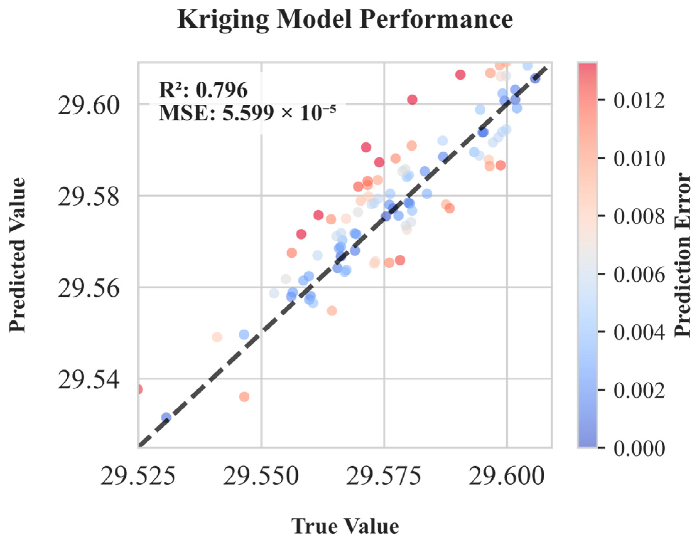
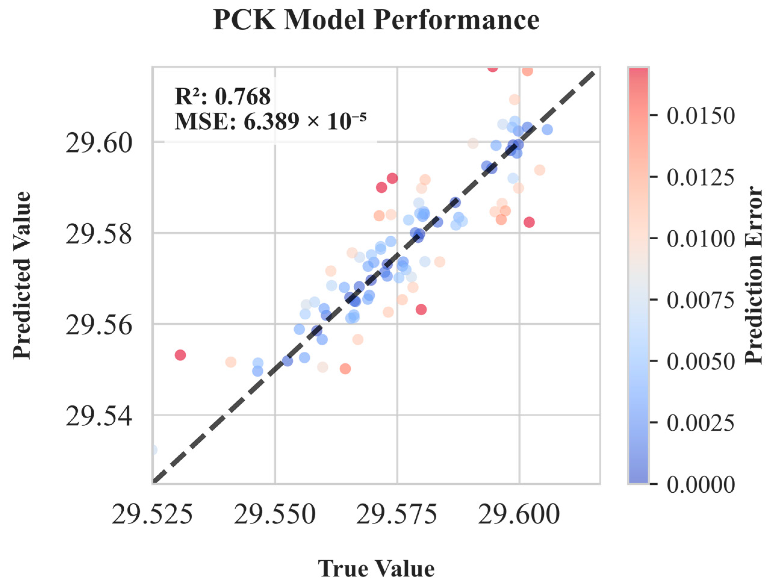
4.2. Comparison of the Precision of Different Surrogate Models

Table 5. Comparison of the blade angle test set errors under different surrogate model methods.

Method	${\mathit{R}}^2$	$\mathit{M}\mathit{S}\mathit{E}$
DNN	0.951	1.4 × 10−5
SVR	0.872	3.53 × 10−5
Kriging	0.796	5.599 × 10−5
RF	0.855	3.992 × 10−5
PCK	0.768	6.389 × 10−5

presents the $R^2$ and $MSE$ for five models, with the DNN model showing significantly better performance metrics compared to other surrogate models.

The above figures (Figure 11, Figure 12, Figure 13, Figure 14 and Figure 15) intuitively illustrate the relationship between model predictions and true values. The further the data points deviate from the line, the greater the difference between the model predictions and the true values. The color of the data points represents the magnitude of the prediction error, with colors leaning toward red indicating larger errors. It is evident that the DNN model’s predictions deviated less from the true values compared to the other surrogate models.

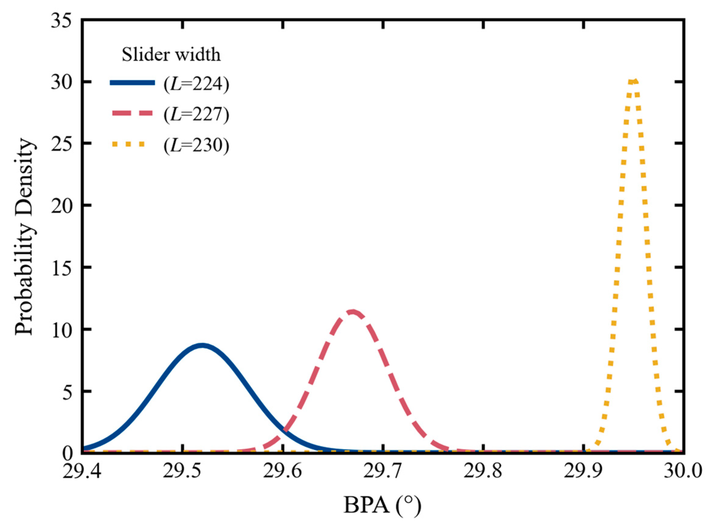
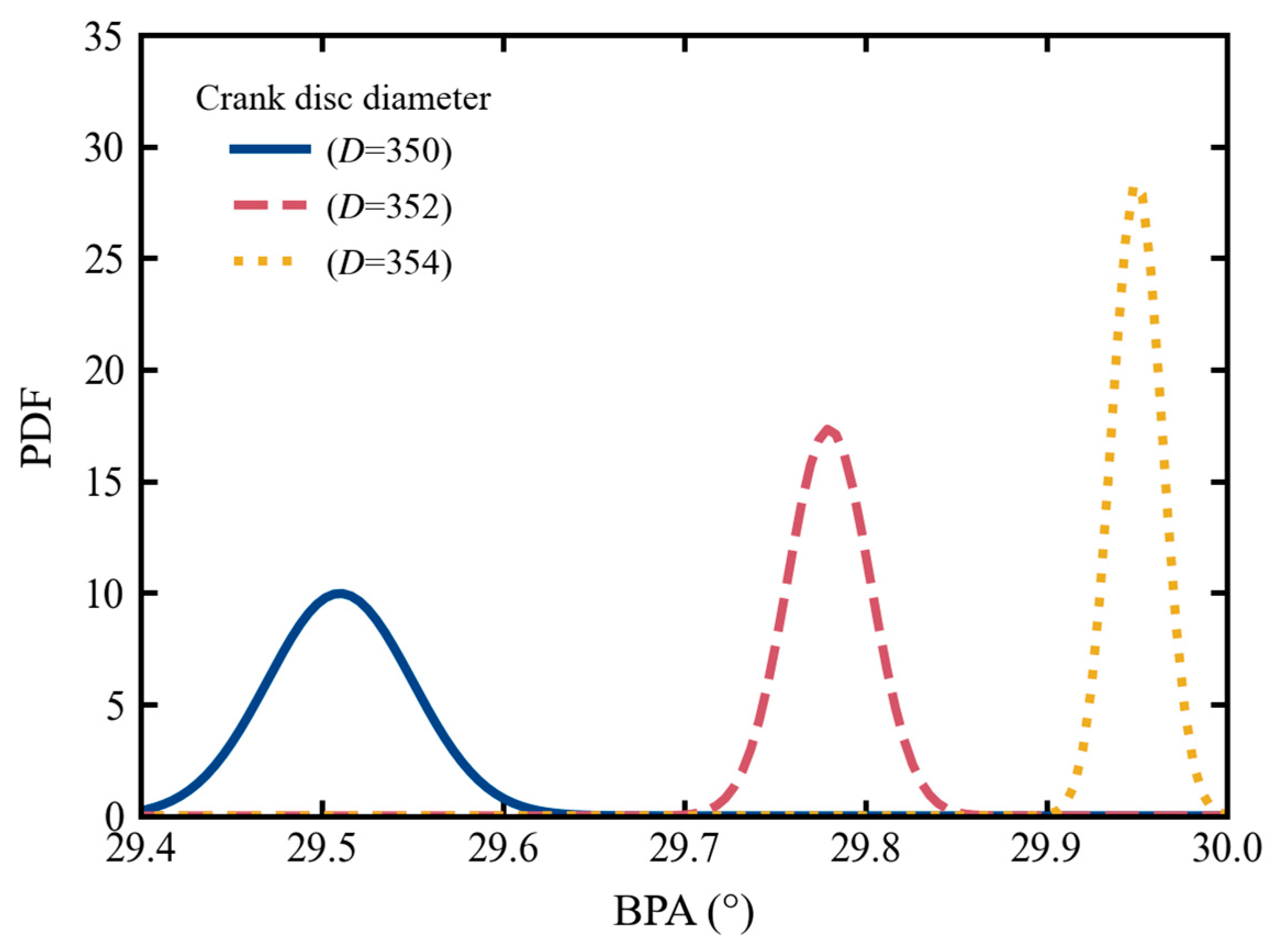
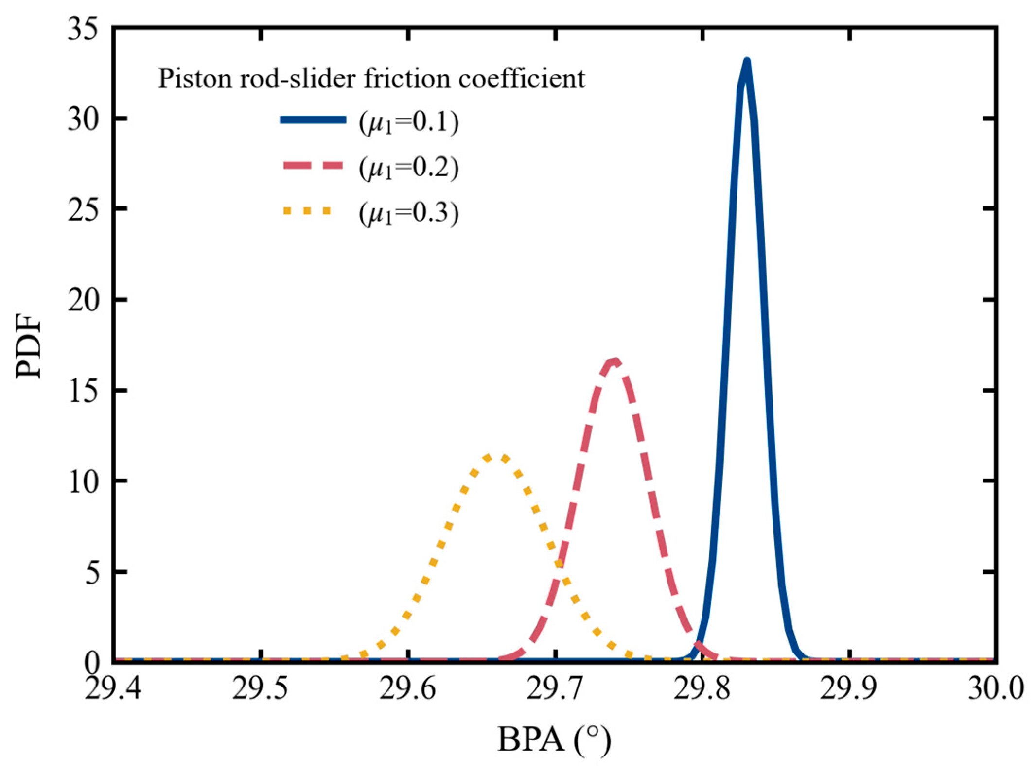
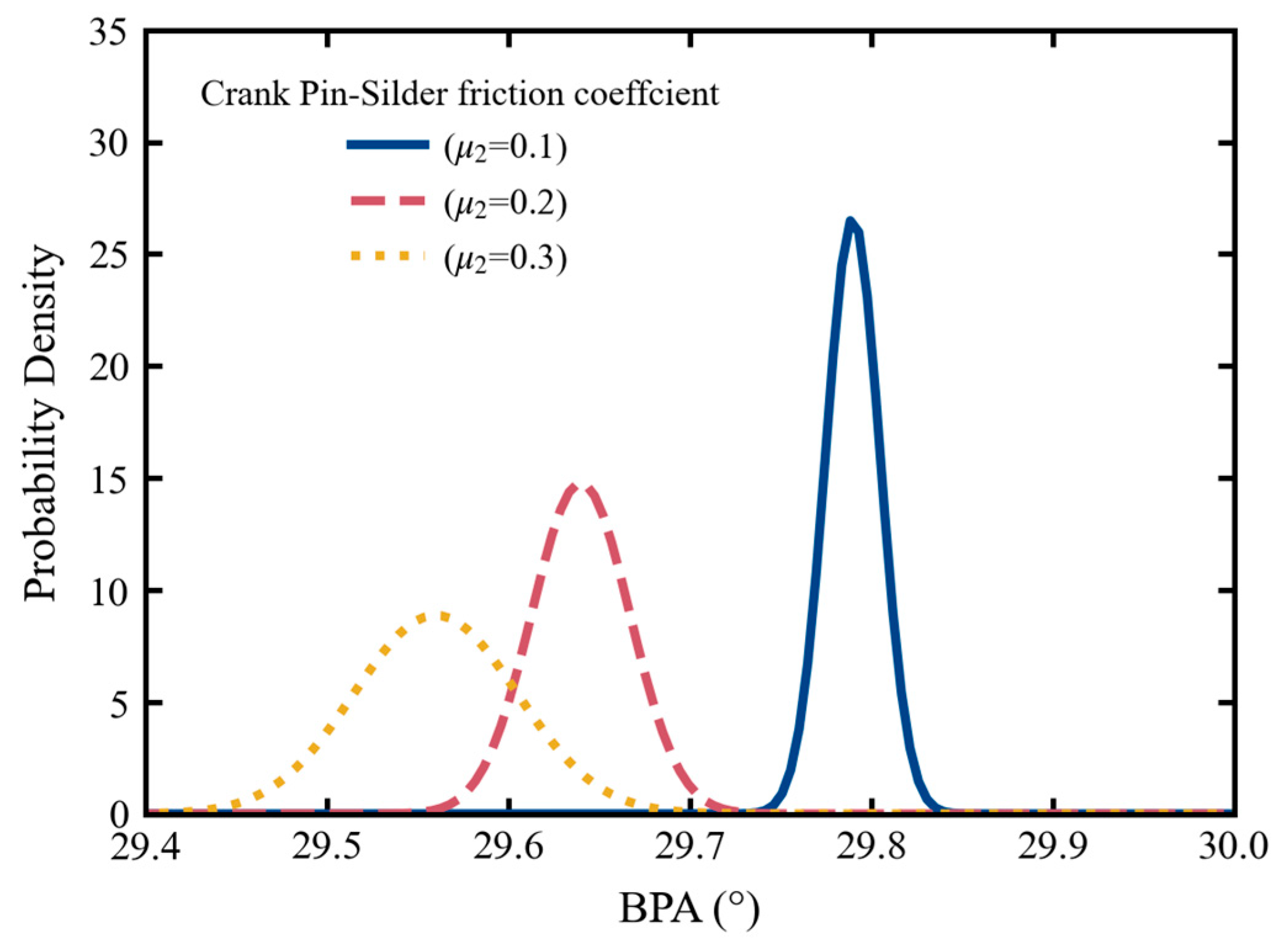
4.3. Results of Uncertainties on the BPA

Figure 16 displays the effect of slider width on BPA, with mean slider widths of 224 mm, 227 mm and 230 mm, as well as a corresponding coefficient of variation of 0.03. In addition to the slider width, the means of the other five variables were, 75 mm, 354 mm, 0.15, 0.15, and 0.15, respectively, with a coefficient of variation of 0.03 for each. Figure 16 illustrates that an increase in the slider width corresponded with a rise in the mean of the BPA distribution, and this was accompanied by a decrease in its standard deviation. This trend indicates that, as the slider width increases, the impact of the uncertainty related to the slider width on the BPA diminishes progressively.

Figure 17 shows the impact of the crank pin diameter on the BPA. The mean values for the crank pin diameter were taken as 71 mm, 73 mm, and 75 mm with a corresponding coefficient of variation of 0.03 for each. Apart from the crank pin diameter, the mean values of the other five variables were 230 mm, 354 mm, 0.15, 0.15, and 0.15, respectively, and their coefficients of variation were also 0.03 each. As shown in Figure 17, with an increase in the crank pin diameter, the mean of the BPA distribution increased slightly, but the standard deviation of its distribution decreased. This signifies that, when the crankpin diameter enlarges, the impact of the uncertainty in the crankpin diameter on BPA progressively lessens.

Figure 18 illustrates the effect of the crank disc diameter on the BPA, where the mean values of the crank disc diameter were set at 350 mm, 352 mm, and 354 mm with a corresponding coefficient of variation of 0.03 for each. Apart from the crank disc diameter, the mean values of the other five variables were 230 mm, 75 mm, 0.15, 0.15, and 0.15, respectively, and their coefficients of variation were also 0.03 each. As shown in Figure 18, as the crank disc diameter increased, the mean of the BPA distribution increased slightly, but the standard deviation of its distribution decreased. This indicates that, as the crank disc diameter increases, the impact of the uncertainty in the crank disc diameter on BPA gradually diminishes.

Figure 19 illustrates the impact of the piston rod–slider friction coefficient on the BPA, with mean values of 0.1, 0.2, and 0.3 for the piston rod–slider friction coefficient, as well as a corresponding coefficient of variation of 0.03 for each. For the remaining five variables, the mean values were 230 mm, 75 mm, 354 mm, 0.15, and 0.15, respectively, with a coefficient of variation of 0.03 for each, as shown in Figure 19. As the piston rod–slider friction coefficient increased, the mean value of the BPA distribution decreased. Notably, its standard deviation also increased. This indicates that, as the piston rod–slider friction coefficient decreases, the uncertainty associated with the piston rod–slider friction coefficient has a progressively smaller effect on the BPA.

Figure 20 illustrates the impact of the crank pin–slider friction coefficient on the BPA, with mean values of 0.1, 0.2, and 0.3 for the crank pin–slider friction coefficient, as well as a corresponding coefficient of variation of 0.03 for each. For the remaining five variables, the mean values were 230 mm, 75 mm, 354 mm, 0.15, and 0.15, respectively, with a coefficient of variation of 0.03 for each, as shown in Figure 20. As the crank pin–slider friction coefficient increased, the mean value of the BPA distribution decreased. Notably, its standard deviation also increased. This indicates that, as the crank pin–slider friction coefficient decreases, the uncertainty associated with the crank pin–slider friction coefficient has a progressively smaller effect on the BPA.

Figure 21 illustrates the impact of the hub bearing–crank disc friction coefficient on the BPA, with mean values of 0.1, 0.2, and 0.3 for the hub bearing–crank disc friction coefficient, as well as a corresponding coefficient of variation of 0.03 for each. For the remaining five variables, the mean values were 230 mm, 75 mm, 354 mm, 0.15, and 0.15, respectively, with a coefficient of variation of 0.03 for each, as shown in Figure 21. As the hub bearing–crank disc friction coefficient increased, the mean value of the BPA distribution decreased. Notably, its standard deviation also increased. This indicates that, as the friction coefficient of the hub bearing–crank disc declines, the uncertainty related to this coefficient increasingly exerts less of an influence on the BPA.

5. Conclusions

This study developed a surrogate model based on DNN to predict the accuracy of the BPA for CPPs, and the results show that, when the slider width is 230 mm, the crank pin diameter is 75 mm and the crank disc diameter is 354 mm; in addition, the friction coefficient of each clearance is lower, leading to the highest reliability of the BPA due to uncertainty factors.

This study established a parametric modeling framework to analyze the influence of the component dimensions and friction coefficients on the BPA of CPP systems. Among the five surrogate models developed, the DNN approach demonstrated superior predictive accuracy, effectively capturing the nonlinear relationships between design parameters and the BPA.

In engineering applications, surface treatment techniques are implemented at critical motion interfaces—specifically, the piston rod–slider, crank pin–slider, and hub bearing–crank disc assemblies—to reduce friction coefficients, thereby mitigating uncertainties in BPA regulation. During CPP operations, periodic maintenance inspections of mechanical clearances are essential. When the clearance exceeds 0.25 mm, experimental observations indicate a corresponding BPA reduction of approximately 0.5 degrees, which significantly compromises pitch adjustment accuracy and propulsion system reliability.

Future research will focus on the uncertainty design of CPPs, obtaining design parameters that enable CPPs to achieve superior motion accuracy through more advanced methods, as well as providing references for the manufacturing of CPPs.

References

1. Tian, W.; Lang, X.; Zhang, C.; Yan, S.; Li, B.; Zang, S. Optimization of Controllable-Pitch Propeller Operations for Yangtze River Sailing Ships. JMSE 2024, 12, 1579. [Google Scholar] [CrossRef]
2. Zhu, W.; Li, Z.; Ding, R. Effect of Pitch Ratio on the Cavitation of Controllable Pitch Propeller. Ocean Eng. 2024, 293, 116692. [Google Scholar] [CrossRef]
3. Bacalja Bašić, B.; Krčum, M.; Jurić, Z. Propeller Optimization in Marine Power Systems: Exploring Its Contribution and Correlation with Renewable Energy Solutions. JMSE 2024, 12, 843. [Google Scholar] [CrossRef]
4. Yurtseven, A.; Aktay, K. The Numerical Investigation of Spindle Torque for a Controllable Pitch Propeller in Feathering Maneuver. brod 2023, 74, 95–108. [Google Scholar] [CrossRef]
5. Pan, W.; Peng, L.; Xing, J. Simulation Study on Controllable Pitch Propeller’s Simulation Based on Virtual Prototype. In Proceedings of the 2011 Second International Conference on Mechanic Automation and Control Engineering, Hohhot, China, 15–17 July 2011. [Google Scholar]
6. Yan, T.; Li, X. The Kinematics Analytical Method and Simulation with ADAMS Based on Bias Slider-Crank Mechanism. Appl. Mech. Mater. 2014, 602–605, 185–188. [Google Scholar] [CrossRef]
7. Dang, Z.; Wu, M.; He, X.; Huang, Z.; Ying, Z.; Chen, Z.; Zheng, C. An Amphibious Propeller Design Optimization Framework Based on Deep Neural Network Surrogate Model. Aerosp. Sci. Technol. 2025, 159, 109967. [Google Scholar] [CrossRef]
8. Gebauer, J.; Wagnerová, R.; Smutný, P.; Podešva, P. Controller Design for Variable Pitch Propeller Propulsion Drive. IFAC-Pap. 2019, 52, 186–191. [Google Scholar] [CrossRef]
9. Wang, J.; Meng, B.; Zhang, L.; Yu, C. Degradation Modeling and Reliability Estimation for Mechanical Transmission Mechanism Considering the Clearance between Kinematic Pairs. Reliab. Eng. Syst. Saf. 2024, 247, 110093. [Google Scholar] [CrossRef]
10. Huang, P.; Wen, C.; Fu, L.; Peng, Q.; Tang, Y. A Deep Learning Approach for Multi-Attribute Data: A Study of Train Delay Prediction in Railway Systems. Inf. Sci. 2020, 516, 234–253. [Google Scholar] [CrossRef]
11. Li, L.; Chen, Y.; Xie, S.; Xiao, Y.; Fang, T.; Wang, C. Comprehensive Feature-Based Machine Learning for Fast Prediction of Marine Propeller’s Open-Water Performance. Appl. Ocean Res. 2025, 154, 104310. [Google Scholar] [CrossRef]
12. Lee, J.; Park, S.-K.; Bazher, S.A.; Seo, D. Development of a Fault Prediction Algorithm for Marine Propulsion Energy Storage System. Energies 2025, 18, 1687. [Google Scholar] [CrossRef]
13. Ye, Y.; Huang, P.; Sun, Y.; Shi, D. MBSNet: A Deep Learning Model for Multibody Dynamics Simulation and Its Application to a Vehicle-Track System. Mech. Syst. Signal Process. 2021, 157, 107716. [Google Scholar] [CrossRef]
14. Kim, J.-H.; Kim, Y.J.; Park, H.-G. Mechanics-Based Machine Learning for Failure Classification of Load-Bearing Walls. Eng. Struct. 2025, 322, 119110. [Google Scholar] [CrossRef]
15. Santos, V.B.; Cardoso-Ribeiro, F.L.; Brugnoli, A. Surrogate Modeling of a Lumped-Mass Multibody Structure Using Hamiltonian Neural Networks. IFAC-Pap. 2024, 58, 48–53. [Google Scholar] [CrossRef]
16. Fan, X.; Yang, X.; Liu, Y. Two-Stage Failure Probability Function Estimation Method Based on Improved Cross-Entropy Importance Sampling and Adaptive Kriging. Reliab. Eng. Syst. Saf. 2025, 263, 111272. [Google Scholar] [CrossRef]
17. Fan, X.; Yang, X.; Liu, Y. A Kriging-Assisted Adaptive Improved Cross-Entropy Importance Sampling Method for Random-Interval Hybrid Reliability Analysis. Struct. Multidisc. Optim. 2024, 67, 158. [Google Scholar] [CrossRef]
18. Tian, W.; Yang, X.; Liu, Y.; Shi, X.; Fan, X. Efficient Damage Prediction and Sensitivity Analysis in Rectangular Welded Plates Subjected to Repeated Blast Loads Utilizing Deep Learning Networks. Acta Mech. 2024, 235, 7223–7244. [Google Scholar] [CrossRef]
19. Han, X.; Liu, L.; Xia, Q.; Liu, D.; Tian, J. Physical-Based Surrogate Model and Its Application in 3D-1D Fusion Optimization of a Marine Two-Stroke Engine. Appl. Therm. Eng. 2025, 271, 126387. [Google Scholar] [CrossRef]
20. Geng, Z.; Zhang, C.; Ren, Y.; Zhu, M.; Chen, R.; Cheng, H. An Uncertainty Weighted Kriging-Random Forest Model for Real-Time Ground Property Prediction during Earth Pressure Balance Shield Tunneling. Appl. Soft Comput. 2025, 180, 113417. [Google Scholar] [CrossRef]
21. Xiao, Y.; Li, X.; Liu, B.; Zhao, L.; Kong, X.; Alhudhaif, A.; Alenezi, F. Multi-View Support Vector Ordinal Regression with Data Uncertainty. Inf. Sci. 2022, 589, 516–530. [Google Scholar] [CrossRef]
22. Liu, B.; Wang, R.; Guan, Z.; Li, J.; Xu, Z.; Guo, X.; Wang, Y. Improved Support Vector Regression Models for Predicting Rock Mass Parameters Using Tunnel Boring Machine Driving Data. Tunn. Undergr. Space Technol. 2019, 91, 102958. [Google Scholar] [CrossRef]
23. Tahir, Z.U.R.; Mandal, P.; Adil, M.T.; Naz, F. Application of Artificial Neural Network to Predict Buckling Load of Thin Cylindrical Shells under Axial Compression. Eng. Struct. 2021, 248, 113221. [Google Scholar] [CrossRef]
24. Nguyen, N.-H.; Nguyen, V.P.; Wu, J.-Y.; Le, T.-H.-H.; Ding, Y. Mesh-Based and Meshfree Reduced Order Phase-Field Models for Brittle Fracture: One Dimensional Problems. Materials 2019, 12, 1858. [Google Scholar] [CrossRef]
Figure 1. Geometric model schematic.
Modelling 06 00054 g001
Figure 2. Hinge collision model.
Modelling 06 00054 g002
Figure 3. Rotary clearance joint model.
Modelling 06 00054 g003
Figure 4. Schematic diagrams of the clearance configuration in controllable pitch propellers.
Modelling 06 00054 g004
Figure 5. Motion patterns of a slider in a piston rod slideway.
Modelling 06 00054 g005
Figure 6. Comparison of the BPA variations under ideal condition and collision model.
Modelling 06 00054 g006
Figure 7. Comparison of the final BPA degrees under multiple clearance configurations.
Modelling 06 00054 g007
Figure 8. A multi-layer DNN model for predicting BPA.
Modelling 06 00054 g008
Figure 9. SVR for regression prediction.
Modelling 06 00054 g009
Figure 10. Diagram of a Kriging/PCK prediction model.
Modelling 06 00054 g010
Figure 11. Comparison of the true and predicted values for the test set of the DNN approach.
Modelling 06 00054 g011
Figure 12. Comparison of true and predicted values for the test set of the SVR approach.
Modelling 06 00054 g012
Figure 13. Comparison of true and predicted values for the test set of the Kriging approach.
Modelling 06 00054 g013
Figure 14. Comparison of the true and predicted values for the test set of the RF approach.
Modelling 06 00054 g014
Figure 15. Comparison of the true and predicted values for the test set of the PCK approach.
Modelling 06 00054 g015
Figure 16. The influence of the slider width on the BPA.
Modelling 06 00054 g016
Figure 17. The influence of the crank pin diameter on the BPA.
Modelling 06 00054 g017
Figure 18. The influence of the crank disc diameter on the BPA.
Modelling 06 00054 g018
Figure 19. The influence of the piston rod–slider friction coefficient on the BPA.
Modelling 06 00054 g019
Figure 20. The influence of the crank pin–slider friction coefficient on the BPA.
Modelling 06 00054 g020
Figure 21. The influence of the hub bearing–crank disc friction coefficient on the BPA.
Modelling 06 00054 g021