Simulating Higher-Dimensional Quantum Communications Using Principal Modes

Abstract

Higher-dimensional communications in optical fiber enables new possibilities, including increased transmission capacity and hyper-entangled state transfer. However, mode coupling between channels during transmission causes interference between channels and limits detection. In classical optical communications, MIMO (modes in modes out) is a means to deal with this issue; however, it is not possible to utilize this technology in quantum communications due to power limitations. Principal mode transmission is another means to deal with mode coupling and signal interference between channels. Conceptually, this can be used in quantum communications with some limitations. In this study, we numerically simulated this process using the time delay method and show how it can be implemented using two and four higher-dimensional quantum states, such as W or GHZ states. These numerical simulations are very illustrative of how the implementation proceeds.

1. Introduction

Higher-dimensional quantum optical communications is a subject of very significant current interest [1,2,3]. It enables the transfer of higher-dimensional quantum states using structured light, enabling more resilient quantum protocols and the investigation of new quantum phenomena, such as hyper-entanglement. Methods for generating hyper-entangled states of light are found in [2]. However, mode coupling between photons traveling in different quantum channels during transmission causes interference between signals and limits detection. Principal mode transmission [4,5] is a means to deal with this limitation and can be implemented with quantum technologies.

A principal mode is a superposition of the N guided modes in a multimode fiber or few-mode fiber [5]. If N guided modes exist within the fiber, there exist N principal modes and the principal modes are a specific superposition of the fiber’s guided modes. The principal modes are orthogonal to each other, and therefore, cross-talk-free transmission can occur using these superpositions. They are independent of frequency to the first order, and this fact can be used to determine these modes [5]. 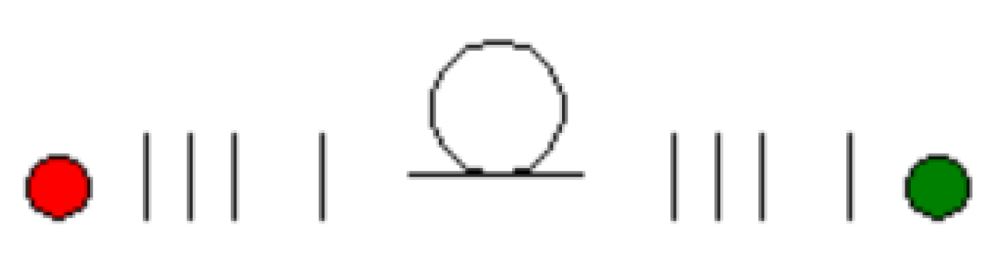Figure 1 is a simplified schematic showing the component figuration required to implement principal state transmission. A source suitable for implementing guided transmission in the fiber is first passed through a lens and a spatial modulator in order to implement the required phase transitions enabling the superpositions of modes. The light is then focused onto the fiber. At the output of the fiber, the superimposed modes are converted back to a specific guided mode or onto a detector. The guided mode can be hyper-entangled. For example, it can contain a specific polarization state and a specific spatial mode. It can then be stored in an appropriate memory for entanglement swapping. Determining these modes is a subject of significant interest and is the subject of Section 2.

Figure 1 is a simplified diagram of the of the component arrangement to implement principal modes in an optical fiber. The order of the components are source, lens, polarization splitter, spatial light modulator, lens, fiber, lens, spatial light modulator, polarization combiner, lens and detector. The principal modes are superpositions of guided modes in the fiber. Methods to generate higher-order modes in optical fiber and superpositions of these modes to form principal modes are documented in the literature. The intent of this publication was to develop the mathematics and algorithms required to implement the propagation and detection of the principal modes. Methods to generate higher-order modes in optical fibers using sources, lenses, polarization components and spatial light modulators have been documented by Berkhout et al. [6] and Lavery et al. [7]. Carpenter [8] showed how to generate principal modes in a fiber that contained 110 modes. The author gives an excellent description of the assembled components.

In a single-mode fiber, there exist two orthogonal polarization states. These two states are not necessarily principal modes, so cross-talk can occur when they are used to multiplex signals. However, principal polarization modes can be determined, and they are used to send information over two separate channels [5,9] without interference. In many quantum communication protocols, a polarization state in a single-mode fiber is used to communicate, and in quantum systems using entanglement swapping, relating the polarization state at the output to the input is necessary [10]. 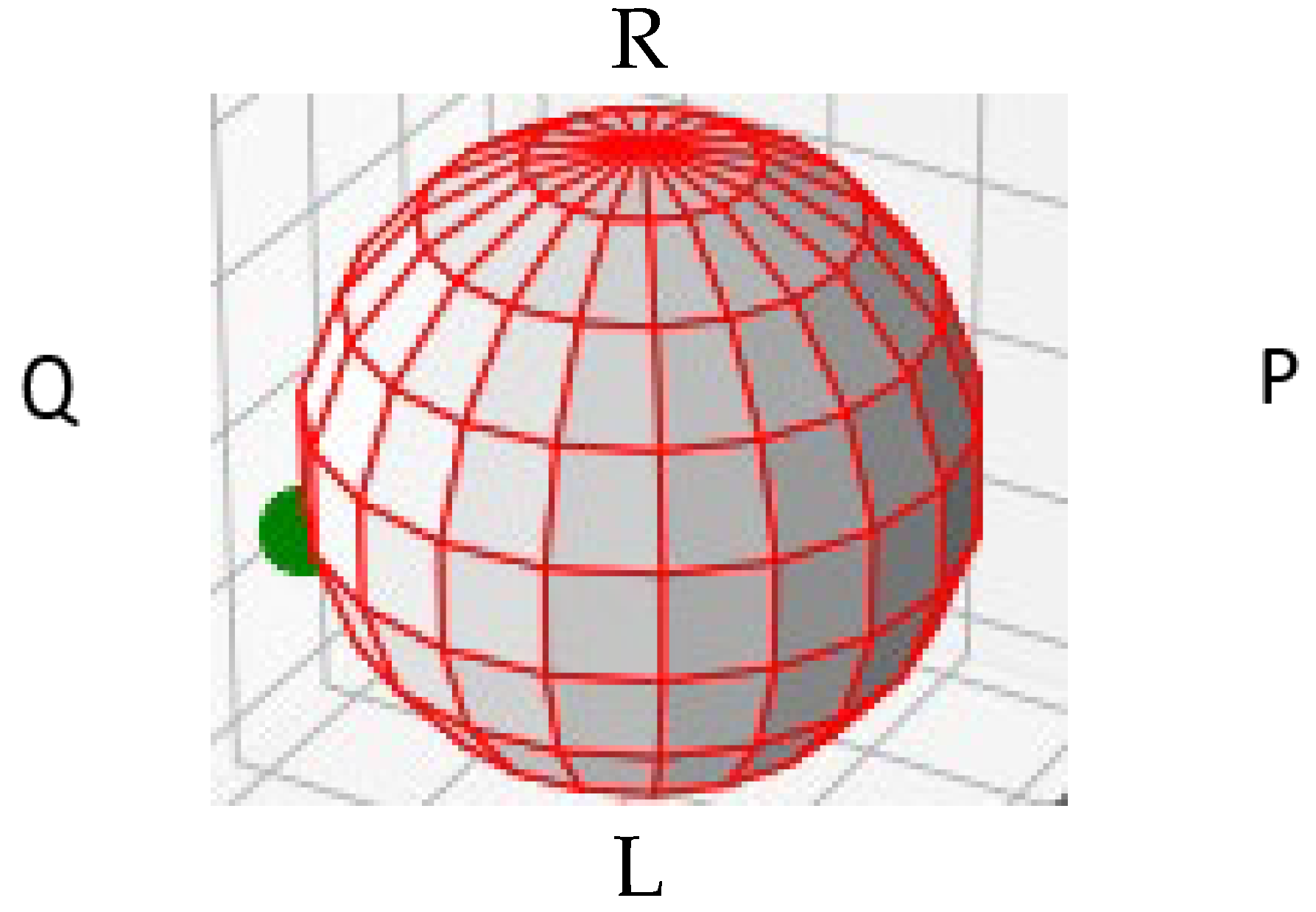Ulrich and Simon [11] theoretically investigated this polarization state evolution in a single-mode fiber. This understanding is critical for tracking the polarization state and its evolution during transmission in quantum communication protocols. They used the Poincare sphere to quantify this evolution. The polarization state in an optical fiber can be linearly, circularly or elliptically polarized, and this state can evolve as the pulse travels in time. The Poincare sphere enables us to display these states, and it is particularly important in relating the input polarization state to that at the output. On the sphere, P and Q represent positions of linear polarization, X and Y, while L and R represents points of circular polarization, left and right. In quantum communication systems, the output polarization is first set to be similar to the input state using classical communications and polarization controllers, which are well-known commercial devices. The output polarization state can drift in time on the order of seconds, so corrections are required. As an example, Figure 2 shows the Poincare sphere with the polarization displayed in a linear state. The notation R, L, P and Q refers to the right-hand circular, left-hand circular, horizontal linear and vertical linear polarization states, respectively.

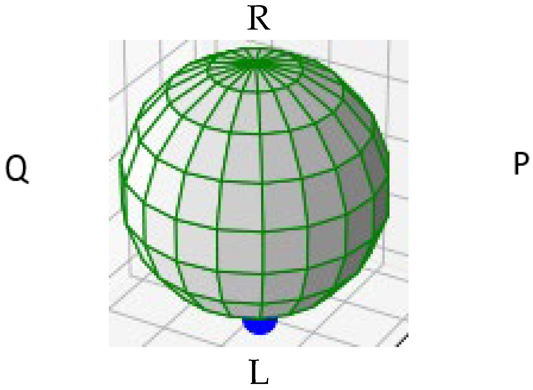
In a multimode fiber, and in the weak guidance approximation, each higher-order-spatial mode contains two polarization states. These spatial modes can be characterized using the well-known linearly polarized modal numbers LPnm [12]. Here, n quantifies the radial modal number and m quantifies the azimuthal number, and also quantifies the orbital angular momentum. Similar to the Poincare sphere, Milione, Sztul, Nolan and Alfano [13] introduced a higher-order Poincare sphere (HOPS) to display these states, as shown below. The colors are arbitrary but are chosen to be different than the Poincare sphere to distinguish between that sphere and the higher-order spatial sphere.

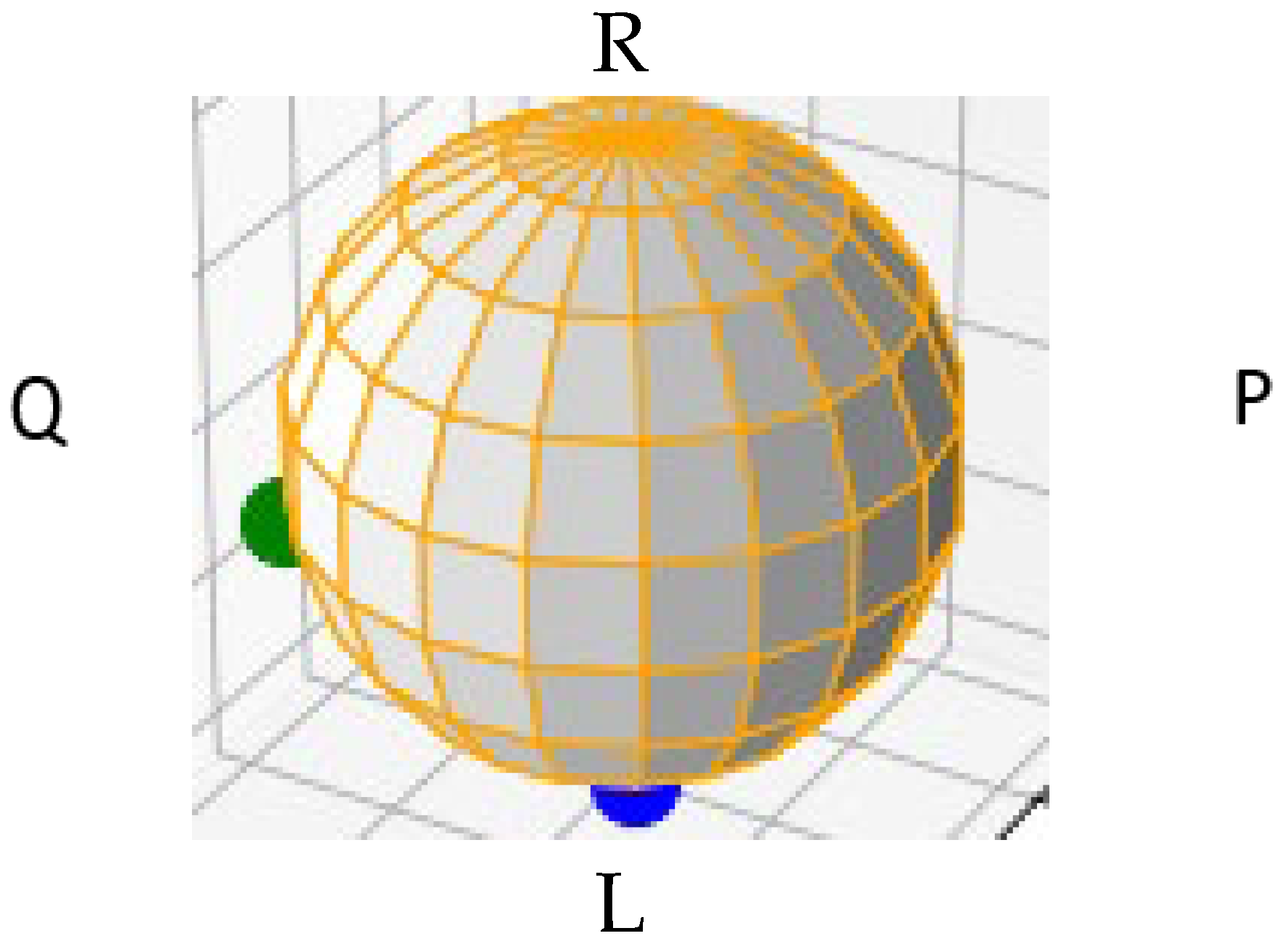
For a specific spatial LPnm mode, this state can be in an OAM (orbital angular momentum) state or it can be in a combination of OAM states, Figure 3. For this reason, it could be in a linear or elliptical state rather than a circular state. For this reason, displaying this mode on the higher-order sphere is very useful. Because spatial modes contain two polarizations, we propose a combined polarization–spatial sphere displaying both spatial and polarization states (Figure 4).

In higher-order quantum communications, when using spatial modes, it is important to recover not only the original polarization state but also the original spatial state. This can be achieved using polarization controllers for the polarization recovery and spatial light modulators to recover the spatial mode. In fact, spatial light modulators can be used to recover both the polarization and spatial states. This is discussed further below. Since the principal modes are orthogonal, one can use them for multiplexing.

2. Principal Modes

The principal modes for multiplexing multimode channels in optical fibers were first proposed by Kahn [4,5]. Carpenter [14] was the first to measure these modes using a few-mode fiber, polarization controllers and spatial light modulators. Using a configuration like the simplified schematic in Figure 1, the author measured a mode transfer matrix, and from this matrix found an approximation to the principal modes of the fiber. The approximation is valid for weak-mode coupling within the fiber. Xiong et al. [15] used a similar experimental configuration and the modal transfer matrix and then determined the principal modes in the case of strong coupling. Using transfer matrices at different wavelengths, they mathematically determined a group delay matrix and subsequently found a principal mode independent of the frequency to the first order. They showed the group delay matrix coincides with the Wigner–Smith time delay matrix, which is important in the study of the fundamentals of electromagnetics.

In a different approach, Milone, Nolan and Alfano [16] proposed a method to determine the principal modes of a fiber using pulse delay data. This work was based on a fundamental paper on polarization mode dispersion authored by Gordon and Kogelnick [17]. In this fundamental paper, they derived an eigenvalue equation to determine the two polarization principal modes propagating at the output of the fiber. In the presence of weak coupling, one can obtain the principal modes at the input by taking the complex of the principal modes at the output. In the case of strong coupling, one needs to send light from the output to the input and calculate the principal modes according to the protocol. The eigenvalues are the two different pulse delays and the eigenfunctions are the principal modes, giving the amplitude and phase of the light to be launched or received. They used SU(2) group theory and the Pauli spin matrices to derive their equations. Milione, Nolan and Alfano generalized this method to N modes using SU(N) group theory and the Gell-Mann general matrices. Later, Nguyen and Nolan et al. [17,18] used this method to experimentally determine the principal modes in a fiber propagating three spatial modes: the LP01 and LP11 modes.

For polarization mode dispersion with two modes, the method requires measuring three different time delays that launch light into three different orientations of the fiber. Each of these orientations contains two different propagating modes with prescribed input phases on these two modes of +1 +1, +1 −1 and +i − i. So, there are three different time delay measurements. Then, using this pulse delay data, one assembles a 2 × 2 eigenvalue matrix. Solving gives the principal mode delays (eigenvalues) and launch conditions (eigenfunctions).

For the case of N modes, the eigenvalue square matrix is (N² − 1) × (N² − 1). There are N² − 1 launch conditions, where each launch condition requires light to be launched simultaneously into multiple modes with defined phases. There are 15 launch conditions needed for a 4 × 4 matrix. These conditions are given in the appendix of reference [13]. These values are appropriate for using the LP11 or LP21 mode to transmit four photons, for example, each photon in a different modal or polarization position. The LP11 mode contains two spatial modes, each of which contain two polarizations. This is the case for all the LPm1 modes in a weakly guided fiber. So, for this reason, the LPM1 modes are useful for transmitting higher-order quantum states, such as GHZ or W states [19]. For example, the GHZ4 state is

$$|GHZ4>={({\displaystyle \frac{1}{2}})}^{0.5}(|0>|0>|0>|0>+|1>|1>|1>|1>)$$

(1)

And the W4 state is

$$|W4>={({\displaystyle \frac{1}{4}})}^{0.5}(|1>|0>|0>|0>+|0>|1>|0>|0>+|0>|0>|1>|0>+|0>|0>|0>|1>)$$

(2)

These states represent qudits, which have a probability amplitude of a photon in a modal slot or not. Each modal position is launched into a principal mode in order to traverse the fiber free of cross-talk. At the output, a principal mode can be projected back onto a specific LPm1 guided mode using a spatial light modulator. The mode can be stored in the optical memory or it can be projected onto a detector.

In Section 3, we show numerically how to assemble a 4 × 4 eigenvalue matrix to solve for the principal modes of the LPm1 modes. We mathematically relate the required 15 launch conditions and measured pulse delay times to the assembled matrix. We then simulate these time delay methods to determine the principal states for two modes, simulating polarization multiplexing in a single-mode fiber, and then determine the principal states in a four-mode fiber simulating the LPm1 modes, containing two spatial modes each with two polarizations. We calculate these modes under the fiber-deployment conditions with imposed mode-coupling sites, and also the situation where the fiber was created using the spin-drawing process. Fiber spinning during the fiber-drawing process is often performed in manufacturing to reduce the polarization mode dispersion.

3. Numerical Simulations to Determine Principal Modes

First, we consider the case for two principal modes. Gordon and Kogelnik [17] showed how to determine these modes using the three Pauli spin matrices to specify the launch amplitude and phases as pulses are launched into the two modes. This gives three time delays and they are determined from the three launches. These time delays Ti are inserted into an eigenvalue matrix, which is assembled by summing the three Pauli spin matrices. The time delays are the measured pulse–peak time delays as measured from the total pulse time delay pulse arrival edge. for the arrival–back edge path. The total pulse launch refers to the unpolarized launch. The eigenvalue matrix components disclosed in their paper are

$$\begin{gathered} H_{00}=T_1 \\ {H}_{01}=T_2-i{T}_3 \\ {H}_{10}=T_2+i{T}_3 \\ {H}_{11}=-T_1 \end{gathered}$$

(3)

As mentioned, solving this equation for the eigenvalues gives the principal mode delays (PMDs), and the eigenfunctions give the launch conditions, phases and amplitudes for the principal mode.

Milione et al. [13] derived these equations for the case of N principal modes, giving a square matrix of size N² − 1. The number of required time delays is also N² − 1. They also list the Gell-Mann matrices for 4 principal modes and 15 matrices in their appendix. This is especially useful for using the LPm1 modes in a fiber containing two spatial modes, each with two polarizations giving four modes. The 4 × 4 eigenvalue matrix components, using the 15 measured time delays and the 15 Gell-Mann matrices, are

$$\begin{gathered} H_{00}=T_3+{\displaystyle \frac{T_8}{3^{0.5}}}+{\displaystyle \frac{T_{15}}{6^{0.5}}} \\ {H}_{01}=T_1-i{T}_2 \\ {H}_{02}=T_4-i{T}_5 \\ {H}_{03}=-i{T}_9+T_{10} \\ {H}_{10}=T_1+i{T}_2 \\ {H}_{11}=-T_3+{\displaystyle \frac{T_8}{3^{0.5}}}+{\displaystyle \frac{T_{15}}{6^{0.5}}} \\ {H}_{12}=T_6-i{T}_7 \\ {H}_{13}=T_{11}-i{T}_{12} \\ {H}_{20}=T_4+iT5 \\ {H}_{21}=T_6+i{T}_7 \\ {H}_{22}+T_{15}/6^{0.5} \\ {H}_{23}=T_{13}-i{T}_{14} \\ {H}_{31}=i{T}_9+T_{10} \\ {H}_{31}=T_{11}+i{T}_{12} \\ {H}_{32}=T_{13}+i{T}_{14} \\ {H}_{33}=-3T_{15}/6^{0.5} \end{gathered}$$

(4)

We used these matrices to simulate several optical fiber deployment conditions. We first considered the situation of two polarization mode transmissions under the situation of an imposed mode-coupling site at 1/4th the transmission distance. We modeled the propagation of these two polarizations through the fibers similar to Matera and Someda [20]. We also considered the case of using spun fiber. We modeled the case of mode coupling in spun fiber similar to that of Li and Nolan [21].

As in [15,16], the polarization fields (i = 1, 2) are written as

$${\displaystyle \frac{d{A}_i}{dz}}=-i\beta A_i+k_{ji} A_j-k_{ij} A_i$$

(5)

We considered the beat length of the fiber to be 1 m with a fiber length of 1 km and a 50/50 mode-coupling site 1/4th the fiber’s total distance; also, the calculated principal mode vectors are of the form a + i b, with the phase θ given by acos(a/(a² + b²)^0.5. If θ = π/2 or 3 π/4, the state is circular and is plotted at the top or bottom vertex of the Poincare sphere. If θ = 0 or π. The state is linear and lies on the equator of the sphere. The principal modes at the fiber output for this mode-coupling situation, characterized as a + j b, were calculated to be

[−0.898 + 0.j          0.275 + 0.342j]
 [−0.275 + 0.342j          0.898 + 0.j]

(6)

It is important to point out that Python 3.11 code does not necessarily return orthogonal eigenstates. If not, one can use the well-known Gram–Schmitt orthogonalization procedure to guarantee orthogonality.

We now investigate the principal modes of a two-mode spun fiber, i.e., two polarization modes. A long-distance single-mode fiber is most often spun during the drawing process as it is fabricated. This is performed to limit the polarization mode dispersion of the fiber [21,22,23,24,25].

In spun fiber, as in [16], the polarization fields (i = 1, 2) are written as

$${\displaystyle \frac{d{A}_i}{dz}}=-i\beta A_i+k_{ji}{A}_j-k_{ij} A_i$$

(7)

For these fibers, the coupling coefficients are of the following forms:

$$\begin{gathered} K_{ij}=0.5\mathsf{\Delta }\beta \mathrm{e}\mathrm{x}\mathrm{p}\left(2iƪ\alpha \left(z\right)dz\right) \\ {K}_{ji}=0.5ᴧ\beta \mathrm{e}\mathrm{x}\mathrm{p}(-2iʅ\alpha \left(z\right)dz) \end{gathered}$$

(8)

Here, α is the spin rate of the fiber. For a fiber of length 100 m and a spin rate of 10 turns per meter, the principal modes at the output of the fiber were calculated to be

[−0.900 + 0.j           0.264 + 0.345j]
 [−0.264 + 0.345j           0.900 + 0.j]

(9)

Then, we considered a four-mode spun fiber using the 15 time delays and the 4 × 4 eigenvalue equations above. This simulated coupling between the LPm1 group modes in a fiber. This group contained two spatial modes, each with two polarizations. Coupling can occur between all the modes. A spatial mode of one polarization can couple to a different spatial mode of a different polarization. As an example, we used two spatial modes, each with two polarizations. We used a beat length of 2 m between the two polarizations of each spatial mode and a beat length of a meter between the spatial modes. The fiber was 100 m long and the spin rate was 10 turns per meter.

The four principal modes were calculated to be

[−0.740 + 0.j    0.409 + 0.240j; 0.198 + 0.258     0.082 + 0.336j]
 [−0.239 + 0.009j   −0.396 + 0.274j; 0.414 + 0.252     0.688 + 0.j]
 [−0.556 + 0.077j   0.648 + 0.j; 0.113 + 0.021     −0.082 + 0.491j]
 [−0.014 + 0.289j  0.202 − 0.100j; −0.505 − 0.118       0.771 + 0.j]

(10)

We used the Python eigen code (la.eig) to solve the eigenvalue equations, which again does not necessarily return orthogonal eigenfunctions.

It is of interest to transmit hyper-entangled states and not necessarily multiplex channels. In this case, one can convert an output principal mode to a state. In qubit-polarization-based quantum key distribution, one recovers the initial input launched polarization at the output. This is achieved not necessarily knowing the output principal state, but knowing this would be helpful. In the four-mode qudit situation, one will similarly need to recover the input qudit state. One can take an output four-mode principal state and project it onto a desired hyper-entangled state using a spatial light modulator. Methods to implement this are disclosed in [6,7,8,26].

4. Outlook

Higher-order dimensional quantum communication is of interest for applications that are related to increased transmission capacity, more resilient to noise and involve the transfer of hyper-entanglement. Methods for generating hyper-states of light can be found in [2]. Mode coupling is a serious issue, and the principal mode-transfer methods discussed in this report can deal with this problem. Beyond these theoretical considerations, new telecommunication-worthy robust devices and components, such as compact spatial light modulators, polarization controllers and metasurface-based lenses, will help hasten this implementation. These components exist and work well in the laboratory but are not yet tested enough for telecommunication deployment. In this report, we focused on mathematical methods and algorithms to determine the principal modes from pulse time delay measurements. The required temporal resolutions exist but are not yet demonstrated for the span of possible pulse delays, for example, short fiber spans. More laboratory demonstrations will help hasten the deployment of higher-dimensional quantum state transmission. Also, the transfer and analysis of hyper-entanglement could lead to new quantum effects.

Hyper-entanglement is a relatively new research topic as it relates to quantum optical communications. Applications using these states, such as implementing quantum optical networks, are new and exciting possibilities [3]. Using OAM modes for the purposes of hyper-entanglement benefits from the very significant worldwide research investigating structured light. The generation of structured light beams [27,28], including the propagation of this light in free space and optical fibers, is of great benefit to the implementation for spatial hyper-entanglement. In addition, there continues to be new understanding and new applications for few-mode and multimode fibers [29,30,31,32,33].

Again, hyper-entanglement is described as photons that are simultaneously entangled in multiple degrees of freedom, such as polarization, frequency, time and/or orbital angular momentum [34]. It can be expected that hyper-entanglement will find applications related to quantum optical networks. Research investigations into quantum network implementations are in an early stage. These implementations include multiply and/or hyper-entangled quantum states [35,36,37]. Methods to generate hyper-entangled states are undergoing significant worldwide research [2] and it can be expected that these methods will continue to expand. Preserving these states as they transmit through an optical fiber is challenging while using, for example, polarization and orbital momentum. Polarization entanglement alone is often used for entanglement transfer in optical fiber but requires the use of polarization controllers, as the state of polarization changes in time as the transmitting polarization evolves on the order of seconds. Polarization controllers enable one to convert to the original polarization at the input to the same polarization at the transmission output. Telecommunication-worthy controllers are already commercially available.

In this paper, we addressed the issue of using both orbital momentum and polarization to transmit hyper-entangled states. Now, one needs to obtain the initial hyper-entangled state at the fiber output, as it has been altered by mode coupling during transmission. This coupling includes both polarization coupling and orbital angular momentum coupling. As mentioned above, principal mode transmission enables one to unscramble the effects of the mode coupling. Using principal modes at the input and output, one can eliminate any mode-coupling distortions. One converts an input entangled state to a principal mode, transmits the principal mode through the fiber and converts the output principal mode to an output hyper-entangled state. In this study, we developed algorithms that enable such a transfer, including how to launch the input and detect the output principal states. We then simulated a transmission experiment under various mode-coupling conditions using the mode propagation equations. We then, using the developed algorithms, showed how to recover the initial hyper-entangled conditions. These algorithms can now be directly applied to experimentally demonstrate the transmission of hyper-entangled (polarization and OAM states) through optical fiber, thereby enabling the successful transfer of polarization–OAM entangled states.