1. Introduction
For rendering visible transparent structures, researchers have used several optical techniques. Applications abound in optical microscopy, optical testing and in fluid dynamics [
1,
2,
3,
4]. Foucault proposes the use of a knife-edge for visualizing departures of sphericity in mirrors and lenses [
5]. Provided that the optical system generates nearly spherical waves, the knife-edge has a high sensitivity when detecting phase gradients.
Toepler employed a knife-edge for visualizing changes in the density in a fluid [
6]. Toepler’s contribution initiated the field of Schlieren techniques, which can detect angular deflections of a parallel beam. Schlieren techniques generate irradiance distributions that are proportional to the first partial derivative of fluid density. In reference [
7], there is an overview of density-sensitive visualization techniques.
For generating irradiance distributions that are proportional to the fluid’s density, one commonly uses interferometric methods. If the density variations produce weak angular deflections, one can use Zernike’s phase contrast technique [
8]. Under the assumption of weak phase delays, this technique generates irradiance distributions that are proportional to the fluid density. Independently of Zernike, Lyot proposed a phase contrast technique for visualizing weak polishing inhomogeneities in a coronagraph [
9].
Advanced Schlieren techniques have benefited from improvements in digital photography, as well as from developments in computer algorithms [
10,
11,
12]. Further improvements are associated with the use of bright white-light sources, and the incorporation of suitable spatial filters. In reference [
13], the authors describe a method that helps to increase the dynamic range of a detector. For a good description of quantitative Schlieren techniques, readers are referred to reference [
14].
Our current discussion does not intend to make comparisons between well-described Schlieren techniques. Here, for visualizing phase gradients, we are proposing to employ the autocorrelation function of a suitably selected coded mask. For our rationale, we describe a simple scalar diffraction treatment, which provides a method for coding the source and for coding the spatial filter. We point out that there are numerical sequences that are useful for obtaining highly peaked autocorrelations. Consequently, there are sets of coded masks that can be applied for visualizing phase gradients. The use of the autocorrelation of a coded mask may help to increase the light gathering power of the Schlieren techniques.
As is common in Fourier optics, transfer functions are often discussed using gratings. As a natural extension, we employ nonconventional transfer functions that can describe the visualization of phase gratings. The discussions based on the use of gratings are regularly associated with deterministic signals. Here, we show that the use of an autocorrelation function (for visualizing phase gradients) is also valid when describing randomly located phase prisms.
In what follows, we unveil the use of a pair of optical masks for implementing a nonconventional Schlieren technique. Our proposal exploits the generation of highly peaked autocorrelation functions. To this end, we employ masks coded with the Barker sequences [
15]. Equivalent results can be achieved by using pseudorandom sequences [
16]. Our proposal does not include experimental verifications. Schardin used grids of transparent and opaque lines as coded light sources [
17], and Jeffree used multiple color-coded slits as a light source with a grid cutoff [
18]. However, these 2D methods are not based on an optical autocorrelation.
For developing our proposal, we make the following assumptions: (a) we assume that an extended source plane is under coherent illumination; (b) phase gradients are described in terms of either a weak phase grating, or of a randomly located prism; (c) we use a nonconventional transfer function, as proposed by Menzel et al. [
19,
20,
21,
22,
23,
24,
25]. The nonconventional transfer function maps the Fourier components of the phase gradient into the Fourier components of an irradiance distribution.
In
Section 2, we revisit the use of an effective transfer function [
26,
27]. In
Section 3, we discuss a simple statistical model of phase gradients. This statistical treatment is in good agreement with a treatment of deterministic signals. In
Section 4, we discuss the use of an autocorrelation function between a coded source and a coded spatial filter. This autocorrelation is described by an integral transformation, which is like those used in phase-space representations [
28,
29,
30,
31,
32,
33,
34,
35]. In
Section 4, we make some numerical comparisons between the autocorrelations obtained using pseudorandom sequences or those attained with the Barker sequences. In
Section 5, we summarize our contributions.
2. A Nonconventional Transfer Function
In
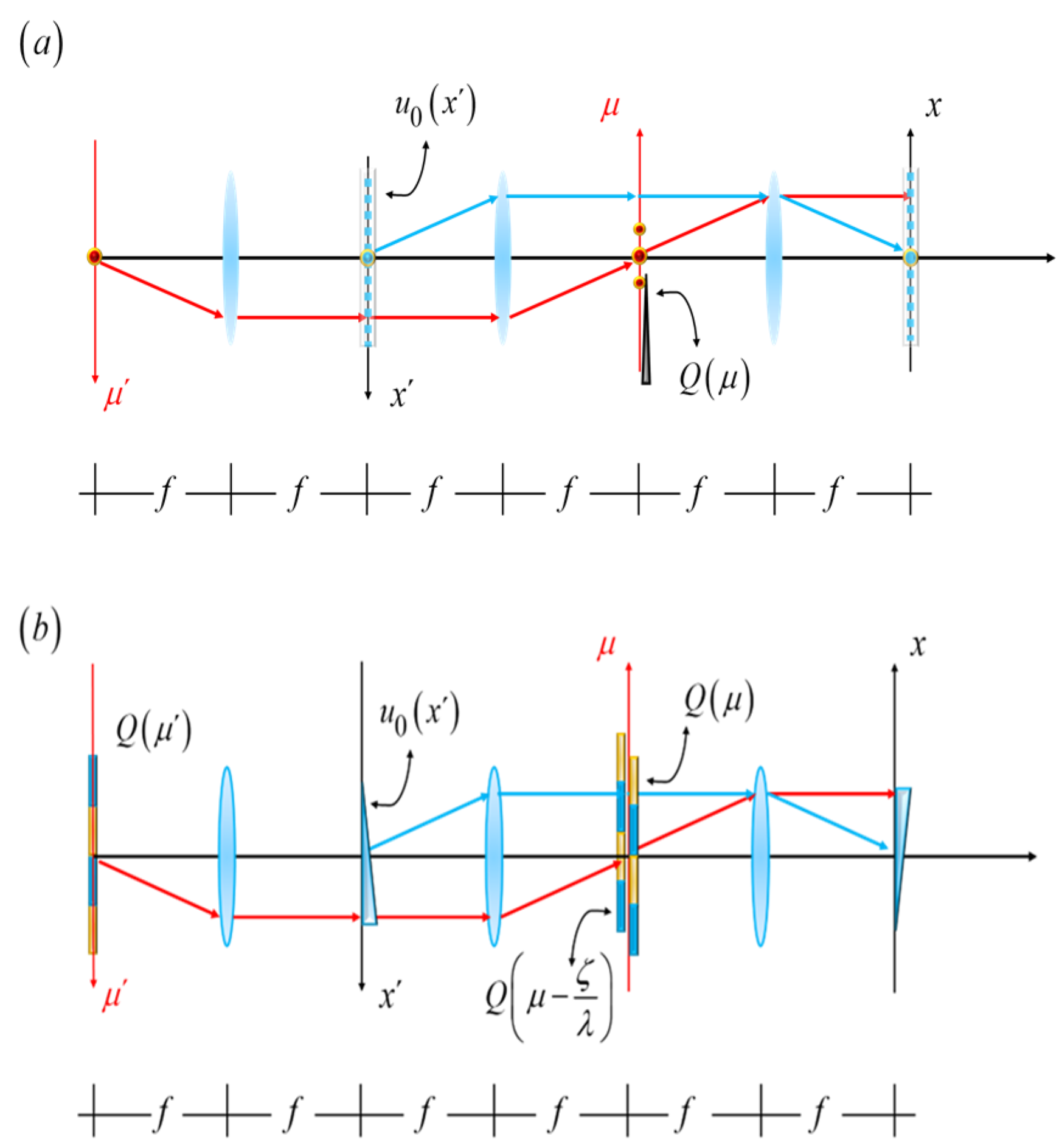
Figure 1, we show the schematics of an optical processor that depicts our proposal.
In
Figure 1b, a phase gradient is placed along the axis x’. Now, as a phase gradient, we consider a sinusoidal phase grating. The sinusoidal phase variations have in amplitude “a”, and a period “d”. The proposed complex amplitude transmittance is
In Equation (1), the lower-case Greek letter λ denotes the wavelength. It is convenient to consider that the grating has weak phase variations, which are
Under this assumption, Equation (1) can be approximated by two terms of a Taylor expansion. Then, the phase structure has a complex amplitude distribution that reads
The Fourier spectrum of Equation (2) is:
In Equation (3), the Greek letters, μ and ν, denote the spatial frequencies at the Fourier domain. In Equation (3), the mathematical expression represents the complex amplitude distribution that impinges on the spatial filter. If the amplitude transmittance of the spatial filter is
, then after the spatial filter, the amplitude transmittance reads
By taking an inverse Fourier transformation of Equation (4), we obtain the complex amplitude distribution at the image plane:
Here, we recognize that in a unique manner
can be expressed as the sum of two functions. The function
is an even function. And the function
is an odd function. For further details, see
Appendix A.
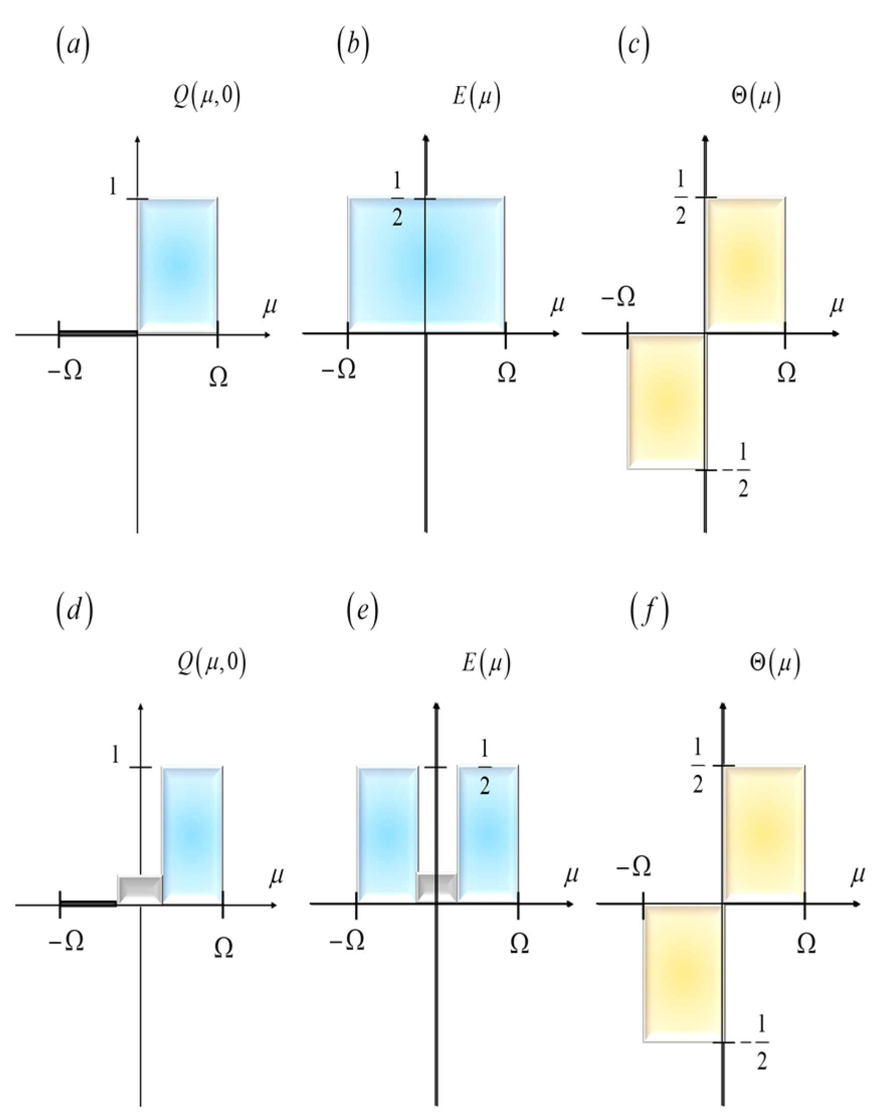
In
Figure 2, we depict the even component,
, and the odd component,
, associated with the amplitude transmittance of two spatial filters
If we substitute Equation (6) in Equation (5), we obtain
We define the normalized image irradiance as
From Equations (7) and (8), we obtain that the normalized image irradiance distribution is
Now, it is relevant to make the following comparison between Equations (2) and (9). The complex amplitude distribution, in Equation (2), is mapped as the image irradiance distribution in Equation (9). Equivalently, the initial sinusoidal variation is transferred as a cosinusoidal variation, with a modulation that is equal to
As depicted in
Figure 3, there is a spatial frequency mapping, which can be associated with an effective transfer function.
It is apparent from Equation (10) that the action of effective transfer function can be enhanced by reducing the transmittance at the center of the spatial filter. This observation is useful for proposing two nonconventional Schlieren techniques. Next, we consider Wolter’s phase-edge [
27]. Its amplitude transmittance is
In Equation (11), the Greek letter Ω denotes the cut-off spatial frequency. In
Figure 4a, we plot Equation (11). For the modulation contrast technique, the amplitude transmittance is
In Equation (12), the Greek letters α and ε denote two real numbers that have values lower than unity. The letter α represents an attenuation coefficient at the center of the mask and the letter ε indicates the fraction of the length associated with the central section. And the letter ε indicates the fraction of the length associated with the central section.
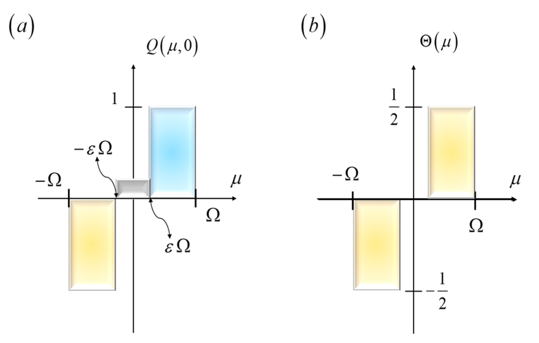
In
Figure 4, we plot the amplitude for an improved version, which incorporates a transmission equal to minus unity; as in Wolter’s phase edge [
27]. And it also incorporates a central attenuation coefficient, as in the modulation contrast technique. Its amplitude distribution reads
For grounding our above description, we simulate a phase gradient as a weak phase grating. Then, it is natural to ask whether the above results are valid for other types of phase gradients. We will answer this question in the next section.
3. Random Phase Gradients
We note the existence of heuristic descriptions for considering a transparent structure as a set of randomly located prisms. Each prism deflects a parallel beam. Then, a knife-edge can block the undeflected beam, allowing the passing of the deflected beam. In this manner, one can visualize the presence of a phase gradient.
This heuristic description ignores any discussions on scalar diffraction. For rectifying this limitation, next we develop a simple statistical model. As depicted in
Figure 5, we consider a set of prisms. Each prism has a random deflection angle ζ. Each member of the set is randomly located at the position X. The prism has a length equal to L. Then, its associated optical signal is:
Equivalently, Equation (14) can be written as
The statistical variations in
X are described by the probability density function
pX(
x). The Fourier transform pair of function p
X(
x) is the characteristic function Φ
X(
µ), namely
Now, the Fourier spectrum of Equation (15) is the amplitude impulse response of the optical system in
Figure 5,
As the value of L increases, the amplitude impulse response can be approximated as
Along the µ’-axis we place a coded mask. Its amplitude transmittance is Q(µ’). The µ-axis is the geometrical optics conjugate of the µ’-axis. At the image conjugate, one can use Equation (18) for obtaining the following complex amplitude distribution
By substituting Equation (18) in Equation (19), we obtain
Next, it is convenient to evaluate the ensemble average of Equation (20). That is,
By substituting Equation (20) in Equation (21), and using the definition of the characteristic function, we obtain
Since the complex amplitude distribution in Equation (22) impinges on the coded mask Q(ζ), just behind this mask the complex amplitude distribution is
The 2D Fourier transform of Equation (23) reads
In Equation (24), the integrand contains two mathematical operations. As in the autocorrelation function, the integrand contains a product of two laterally shifted signals. The integrand also contains the kernel of a Fourier transformation. This type of integrand appears when evaluating phase-space representations. For signals that evolve in time, a phase-space representation displays simultaneously the variations in time and in the temporal frequency. For signals that evolve in the space domain, a phase-space representation simultaneously displays the position and the spatial frequency. The Wigner distribution and the ambiguity function are two examples of these representations [
28,
29]. In fact, the Wigner distribution and the ambiguity function are Fourier transform pairs. Phase-space representations are useful in several branches of applied optics [
30,
31,
32,
33,
34,
35]. Any further discussions on this topic are beyond our current scope.
For the sake of completeness of our discussion, in the next section, we describe a deterministic treatment. The deterministic model has good agreement with the above statistical model.
4. Coded Source: A Deterministic Imaging Process
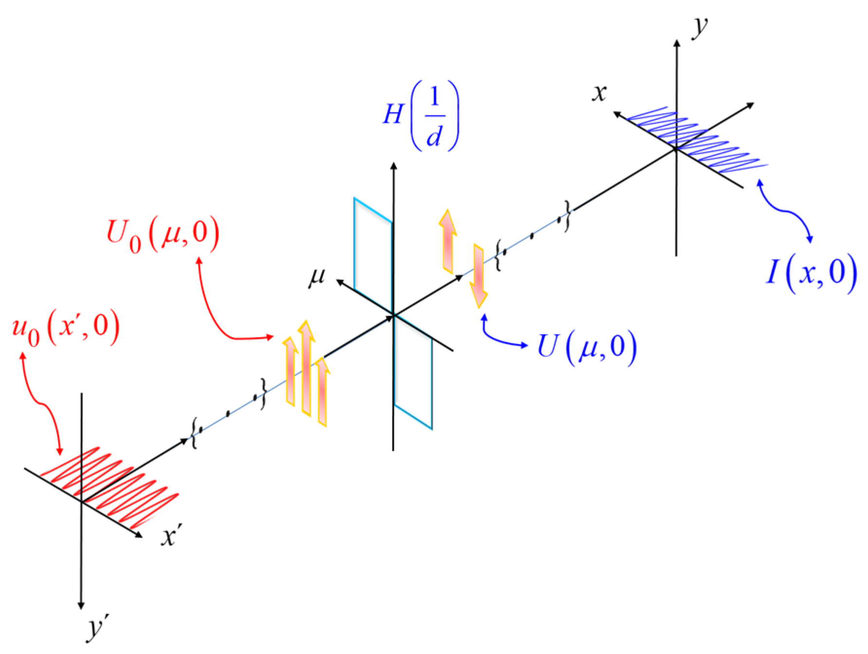
For complementing our previous discussion, on randomly located prisms, next we discuss a fully deterministic treatment. As part of our rationale, first we describe some heuristic arguments. As depicted in
Figure 6, we contemplate a coherently illuminated slit. At its conjugated image, (μ, ν), we place a second slit that acts as the spatial filter.
In the absence of phase gradients, the two slits coincide, and the light throughput achieves its maximum value. On the other hand, if a phase gradient is present then the image of the source is laterally shifted (say by the amount
ζ/λ). This mismatch generates a drop in light throughput. That is,
In Equation (25), the Greek letter Ω denotes the width of the slit that is used to cover the source. If one evaluates Equation (25), then one obtains:
It is apparent from Equation (26) that the light throughput varies slowly with the variable
ζ, except for a very narrow slit. However, the light throughput is reduced if one uses narrows slits. Hence, we search next for other options. To conclude, we consider that the source is coded with multiple slits. Then, at the source plane, the amplitude transmittance is:
In Equation (27), the Greek letters μ’ and ν’ denote spatial frequency coordinates at the source plane. At the input plane, the coordinates we employ the coordinates
x’ and
y’. At this plane, the amplitude distribution is the Fourier transform of Equation (30). That is,
In Equation (28), the function
is the 1D Fourier transform of the coded source. Next, we consider that a prism alters the amplitude distribution in Equation (28). Then, the new amplitude distribution reads
In Equation (29) we consider the presence of a phase gradient, with deflection angle
ζ. At the pupil aperture, the amplitude distribution is the inverse Fourier transform of Equation (29). That is,
Next, we consider that the amplitude distribution, in Equation (30), impinges on a second coded mask. The second coded mask acts as the spatial filter. Its amplitude transmittance is
Q*(
μ). Then, just after the mask, the amplitude transmittance is
It is straightforward to substitute Equation (30) in Equation (31), for obtaining:
As expected, at the pupil aperture, the amplitude distribution is the product of a laterally shifted version of the coded mask times the complex conjugate transmittance of the mask that acts as the spatial filter. Consequently, at the image plane, the amplitude distribution is
As in Equation (24), the mathematical expression in Equation (33) describes an integrand that contains two mathematical operations. It contains the product of two laterally shifted signals. The integrand also contains the kernel of a Fourier transformation. As previously pointed out, the integrand is like those employed when evaluating phase-space representations. Here, we concentrate on the use of Equation (33), if it is evaluated at the origin (
x = 0,
y = 0). Hence, we are currently interested in the following equation
Using Equation (34), we advance the following working hypothesis: if the source and the spatial filter are coded with the same sequence, then one can optically implement an autocorrelation operation. This autocorrelation can be usefully applied to the automatic detection of phase gradients. This working hypothesis is discussed in what follows.
5. Optical Visualization and Automatic Detection
The pseudorandom sequences and the Barker sequences can generate highly peaked autocorrelations. Then, they are good candidates for coding masks that employ the autocorrelation function for detecting phase gradients. For elaborating on this working hypothesis, we note that either the pseudorandom sequences, or the Barker sequences have a finite number of elements, say L. This integer number L is denoted as the sequence length. For applications in electronics, the sequences are used as cyclic sequences. However, in optics, due to the finite size of the mask, the coding sequences are noncyclic. We elaborate on this difference.
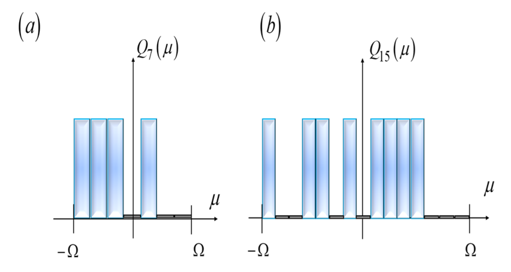
The pseudorandom sequences exhibit a high peak over an otherwise uniform value, as depicted in
Figure 7. The selected sequences have amplitude transmittance that are equal to unity, or equal to zero. Then, they are useful for implementing a Schlieren technique with white light. In
Figure 7a, the length of the pseudorandom is L = 7. And in
Figure 7b, the length is L = 15. These examples are selected for making comparisons with the results in reference [
15].
In
Figure 8, we show the cyclic autocorrelations associated with the sequences in
Figure 7. It is apparent that the autocorrelations exhibit peaks that overshoot a uniform value.
In
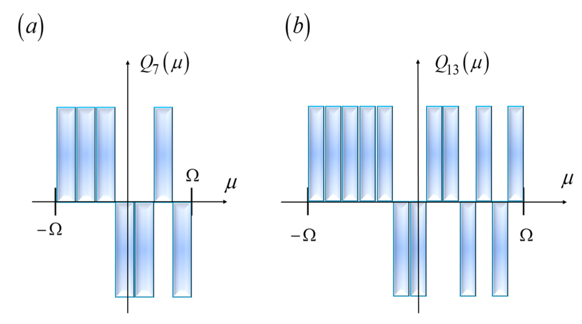
Figure 9, we show Barker sequences of length L = 7 and L = 13. Now, the amplitude transmittance has values that are either equal to unity, or equal to minus unity.
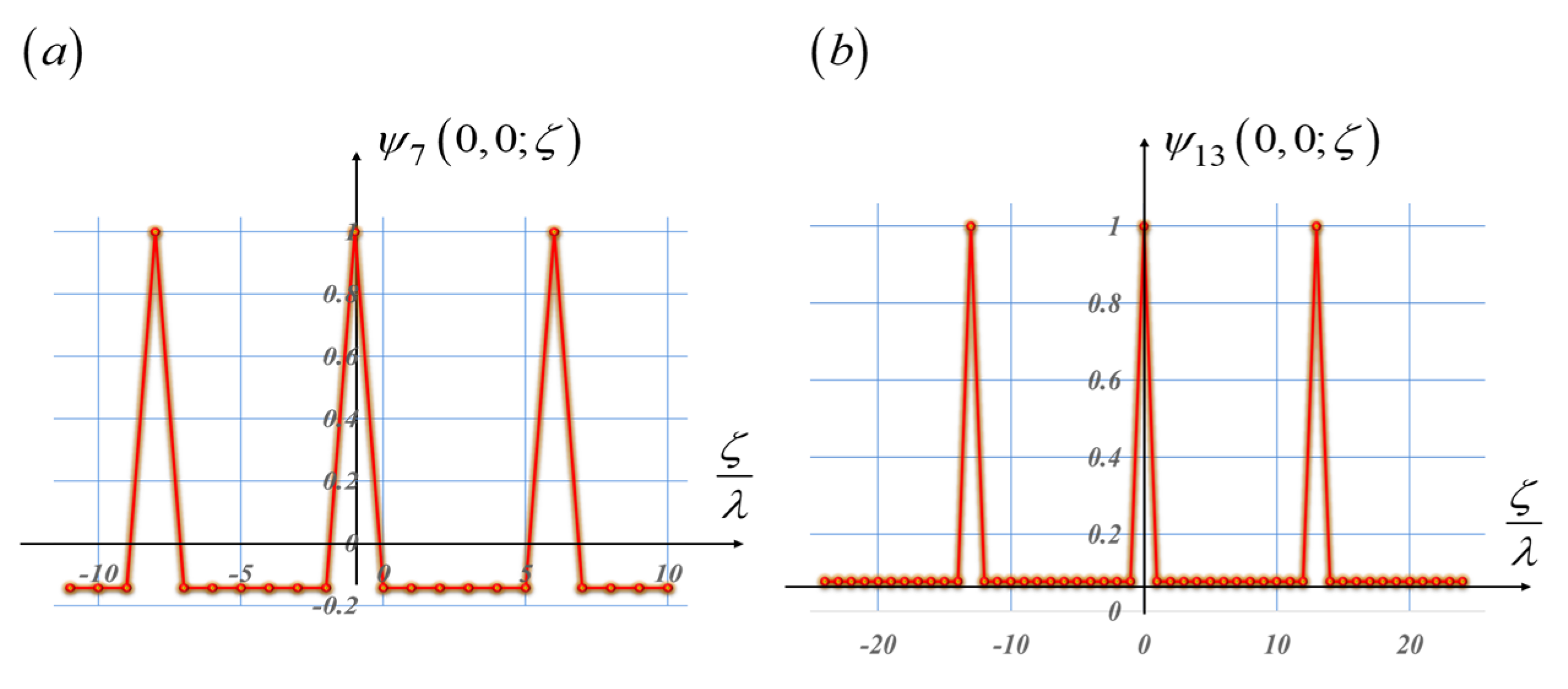
In
Figure 10, we plot the cyclic autocorrelation associated with the sequences in
Figure 9. It is apparent from
Figure 10 that the autocorrelations also have peaks that overrun the values of the adjacent sidelobes. We note that the peaks baselines narrow down, when going from the length L = 7 to the length L = 13.
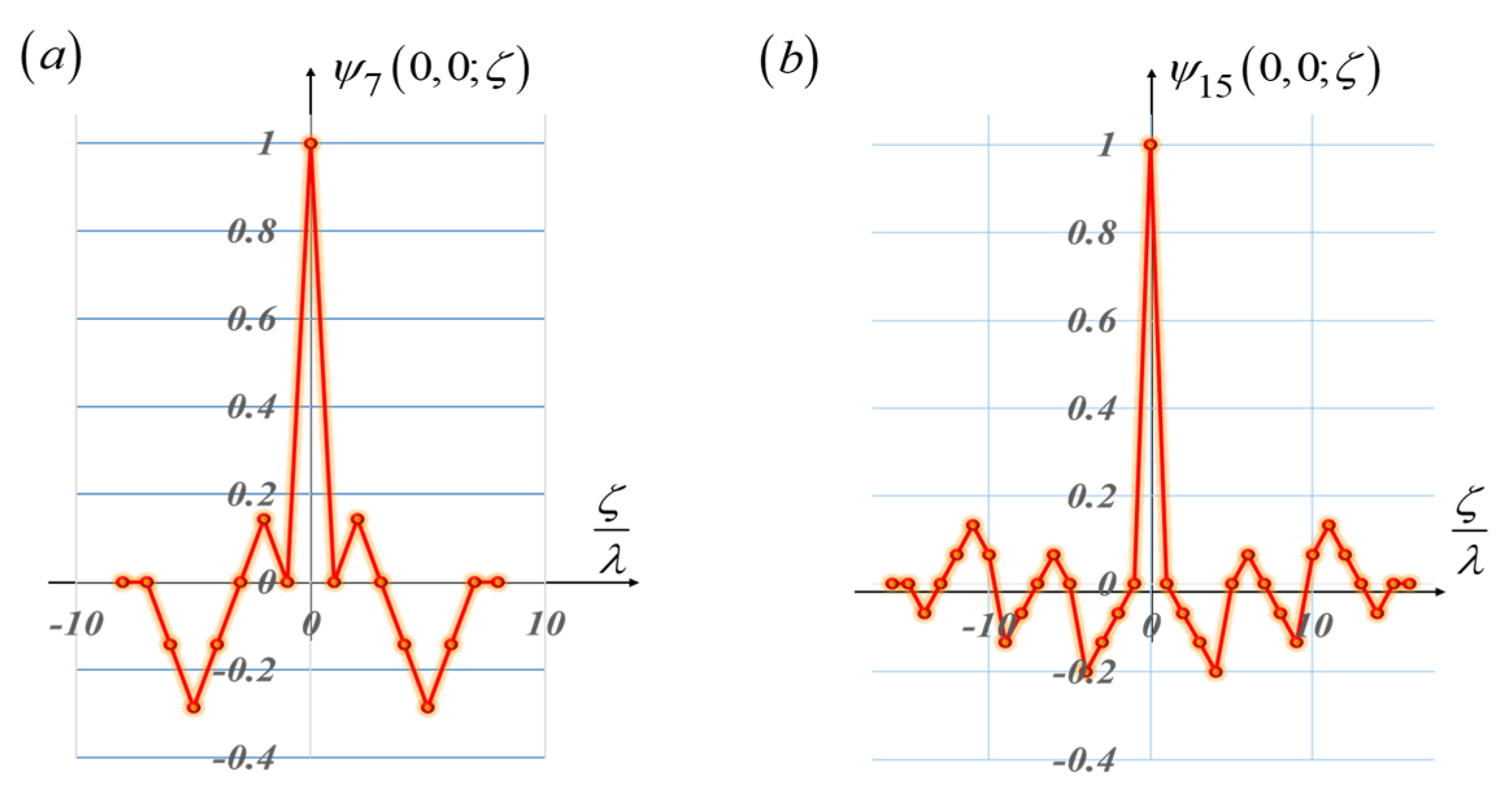
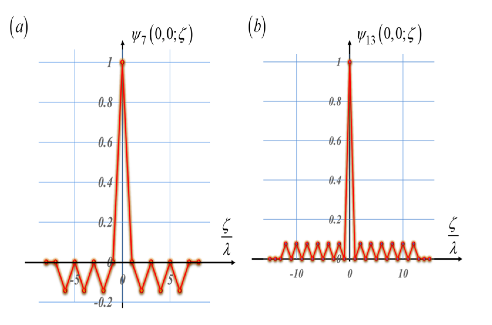
As previously indicated, in optics, one is dealing with noncyclic autocorrelations. This is due to the finite size of the masks. The autocorrelations do not repeat themselves. To visualize the impact of this feature, we present the noncyclic autocorrelations of the pseudo-random sequences, as well as the noncyclic autocorrelations of the Barker sequences. From
Figure 11 and
Figure 12, we note that the noncyclic autocorrelations do not have replicated peaks. Furthermore, associated with the pseudorandom sequences, the noncyclic autocorrelations exhibit sidelobes having variable values.
From
Figure 11 and
Figure 12, we note that the noncyclic autocorrelations do not have replicated peaks. Furthermore, associated with the pseudorandom sequences, the noncyclic autocorrelations exhibit sidelobes having variable values.
From
Figure 12, we observe that the Barker sequences generate noncyclic autocorrelations that exhibit a distinctive central peak, The sidelobes are replicated with equal values. We observe that in the absence of phase gradients, the noncyclic autocorrelations have a central distinctive peak.
Hence, the Barker codes are a desirable choice for implementing an optical autocorrelation sensor. For this purpose,
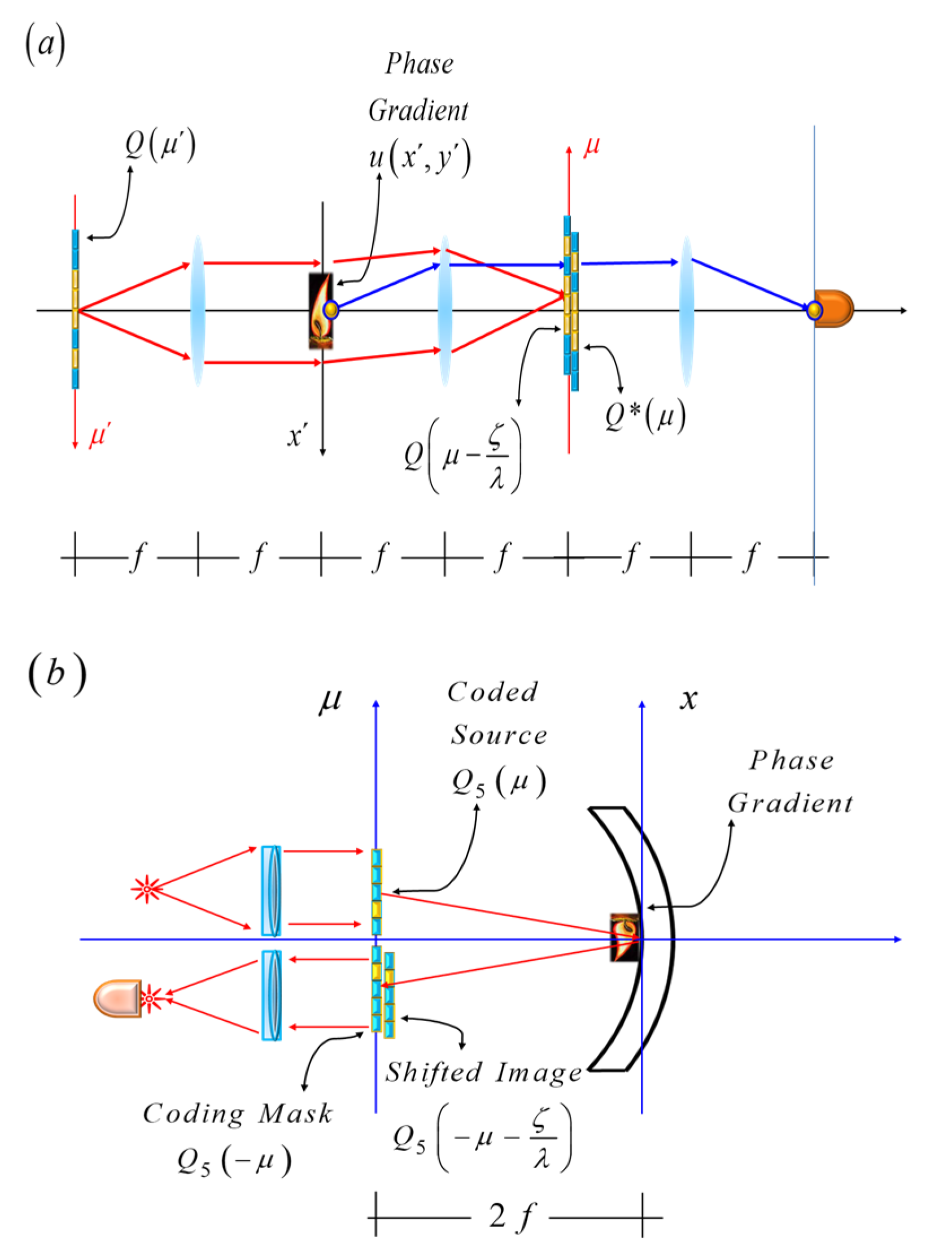
Figure 13 shows the optical setup, with (a) presenting the unfolded version and (b) depicting the folded version using a spherical mirror.
In
Figure 13b, the plane of the phase gradient cannot physically be in contact with the mirror at its center. But it must lie at some small distance in front of the mirror. This then leads to a slight doubling of the phase gradient when a Schlieren image is formed. Finally, we note that the proposed Schlieren technique has not yet been experimentally assessed.
6. Conclusions
We have described a theoretical framework for designing nonconventional Schlieren techniques. To this end, we have revisited the use of an effective transfer function. This discussion clarifies the relevance of employing arguments of symmetry, when designing Schlieren techniques.
We have presented a simple statistical model for describing phase gradients as randomly located prisms. This treatment is in good agreement with a deterministic model, which describes weak phase gradients.
The nonconventional Schlieren techniques employ a pair of coded masks, for implementing an optical autocorrelation. One element of the pair encodes a coherently illuminated plane, which acts as the source. And the second element of the pair acts as the spatial filter. The coded masks are located on geometric–optical conjugate planes.
The described autocorrelator exploits the use of Barker sequences for generating highly peaked, noncyclic irradiance distributions. We have indicated that equivalent results can be achieved by coding the masks with pseudorandom sequences.
The current discussion does not contain experimental verifications of the theoretical framework.
Author Contributions
Conceptualization, J.O.-C.; methodology, J.O.-C.; software, C.M.G.-S.; validation, J.O.-C. and C.M.G.-S.; writing—original draft preparation, J.O.-C.; writing—review and editing, C.M.G.-S. All authors have read and agreed to the published version of the manuscript.
Funding
This research received no external funding.
Data Availability Statement
Currently, we do not include the numerical procedures for evaluating the graphs and the figures in this paper.
Acknowledgments
We are indebted to two anonymous reviewers for their guidance and their many valuable suggestions.
Conflicts of Interest
The authors declare no conflicts of interest.
Appendix A. Symmetry Considerations
As pointed out in Equation (6), we write the amplitude transmittance as the sum of an even function and of an odd function
One finds the even function by using the formula:
By substituting Equation (A1) in Equation (5), in the main text, we have that:
Equation (A4) can also be written as:
Equation (A5) appears as Equation (7) in the main text.
Appendix B. Statistical Considerations
We use a Fourier transform for expressing the even component in Equation (19) as follows:
We note that the function is a real, even function of the variable x. We note that the odd component, in Equation (20), is a real function. Its Fourier transform is also an odd function. However, its Fourier transform is a purely imaginary function. Hence, it is convenient to use the following expression:
Thus, at the image plane, the average amplitude distribution is:
Or equivalently, the average amplitude distribution is:
Next, we use the following definition for the normalized, average irradiance distribution:
By substituting Equation (A9) in Equation (A10) we have that:
Equation (A11) appears as Equation (9) in the main text.
References
- Daria, V.; Glückstad, J.; Mogensen, P.C.; Eriksen, R.L.; Sinzinger, S. Implementing the generalized phase-contrast method in a planar-integrated micro-optics platform. Opt. Lett. 2002, 27, 945–947. [Google Scholar] [CrossRef] [PubMed]
- Teschke, M.; Sinzinger, S. Modified phase contrast for recording of holographic optical elements. Opt. Lett. 2007, 32, 2067–2069. [Google Scholar] [CrossRef]
- Teschke, M.; Heyer, R.; Fritzsche, M.; Stoebenau, S.; Sinzinger, S. Application of an interferometric phase contrast method to fabricate arbitrary diffractive optical elements. Appl. Opt. 2008, 47, 2550–2556. [Google Scholar] [CrossRef] [PubMed]
- Teschke, M.; Sinzinger, S. Phase contrast imaging: A generalized perspective. J. Opt. Soc. Am. A 2009, 26, 1015. [Google Scholar] [CrossRef]
- Foucault, L. Description des procédées employés pour reconnaître la configuration des surfaces optiques. Comptes Rendus Hebd. Des Séances De L’académie des Sci. 1858, 47, 958–959. [Google Scholar]
- Toepler, A. Beobachtungen nach einer Neuen Optischen Methode. Poggendorf’s Ann. Der Phys. Und Chemie 1866, 127, 556–580. [Google Scholar]
- Kleine, H. Measurement Techniques and Diagnostics. In Flow Visualization, Chapter 5, Handbook of Shock Waves; Academic Press: Cambridge, MA, USA, 2001. [Google Scholar]
- Zernike, F. Diffraction theory of the knife-edge test and its improved form, the phase-contrast method. Mon. Not. R. Astron. Soc. 1934, 94, 377–384. [Google Scholar] [CrossRef]
- Lyot, B. Procèdes Perme Hand d’Etudier les Irrégularités d’une Surface Optique Bien Polie. C. R. Acad. Sci. 1946, 222, 765. [Google Scholar]
- Elsinga, G.; Van Oudheusden, B.; Scarano, F.; Watt, D. Assessment, and application of quantitative schlieren methods: Calibrated color schlieren and background oriented schlieren. Exp. Fluids 2004, 36, 309–325. [Google Scholar] [CrossRef]
- Settles, G.S. Schlieren and Shadowgraph Techniques: Visualizing Phenomena in Transparent Media; Springer Science & Business Media: Berlin/Heidelberg, Germany, 2001. [Google Scholar]
- Cwik, A.; Ermert, H. A quantitative schlieren method for the investigation of axis-symmetrical shock waves. In Proceedings of the 1993 Proceedings IEEE Ultrasonics Symposium, Baltimore, MD, USA, 31 October–3 November 1993; pp. 789–792. [Google Scholar]
- Vogel, A.; Apitz, I.; Freidank, S.; Dijkink, R. Sensitive high-resolution white-light schlieren technique with a large dynamic range for the investigation of ablation dynamics. Opt. Lett. 2006, 31, 1812–1814. [Google Scholar] [CrossRef]
- Hargather, M.J.; Settles, G.S. A comparison of three quantitative Schlieren techniques. Opt. Lasers Eng. 2012, 50, 8–17. [Google Scholar] [CrossRef]
- Barker, R.H. Group Synchronizing of Binary Digital Systems. In Communication Theory; Butterworth: London, UK, 1953; pp. 273–287. [Google Scholar]
- Harwit, M.; Sloane, N.J.A. Hadamard Transform Optics; Academic Press: New York, NY, USA, 1979; pp. 200–2005. [Google Scholar]
- Schardin, H. Die Schlierenverfahren und ihre Anwendungen. Ergeb. Der Exakten Naturwissenschaften 1942, 20, 303–439. [Google Scholar]
- Jeffree, H. A wide range Schlieren system. J. Sci. Instrum. 1956, 33, 29–30. [Google Scholar] [CrossRef]
- Menzel, E. Die Darstellung verschiedener Phasekontrast Verfahren in der Optischen Ubertragungstheori. Optik 1958, 15, 460–470. [Google Scholar]
- Menzel, E. Transfer-functions in optics. Optik 1973, 39, 170–172. [Google Scholar]
- Menzel, E.; Mirandé, W. Weingaertner, Fourier-Optik und Holographie; Springer: Wien, Austria, 1973; pp. 77–80. [Google Scholar]
- Slansky, S. Images Partiellement Cohérentes de Faible Contraste. Opt. Acta 1962, 9, 277–294. [Google Scholar] [CrossRef]
- Ojeda-Castaneda, J. A proposal to classify methods employed to detect thin phase structures under coherent illumination. Opt. Acta 1980, 27, 917–929. [Google Scholar] [CrossRef]
- Ojeda-Castaneda, J. Chapter 5, Foucault wire and phase modulation tests. In Optical Shop Testing; Malacara, D., Ed.; John Wiley: New York, NY, USA, 1992; pp. 265–320. [Google Scholar]
- Gómez-Sarabia, C.M.; Ojeda-Castaneda, J. Schlieren masks: Square root monomials, sigmoidal functions, and off-axis Gaussians. Appl. Opt. 2020, 59, 3589–3594. [Google Scholar] [CrossRef]
- Hofmann, R.; Gross, L. Modulation Contrast Microscope. Appl. Opt. 1975, 14, 1169–1176. [Google Scholar] [CrossRef]
- Wolter, H. Schlieren-Phase Kontrast und Lichtschnittverfahren. In Handbuch der Physik 24; Springer: Berlin/Heidelberg, Germany, 1956; pp. 555–645. [Google Scholar]
- Bastiaans, M.J. Chapter 1, Wigner distribution in optics. In Phase-Space Optics; Testorf, M., Hennelly, B., Ojeda-Castañeda, J., Eds.; McGraw-Hill: New York, NY, USA, 2010; pp. 1–44. [Google Scholar]
- Guigay, J.-P. Chapter 2, The ambiguity function in optical imaging. In Phase-Space Optics; Testorf, M., Hennelly, B., Ojeda-Castañeda, J., Eds.; McGraw-Hill: New York, NY, USA, 2010; pp. 45–62. [Google Scholar]
- Hazra, L. Foundations of Optical System Analysis and Design; CRC Press: Boca Raton, FL, USA, 2022; pp. 157–178. [Google Scholar]
- Ojeda-Castaneda, J. Wavefront Shaping and Pupil Engineering; Springer: Berlin/Heidelberg, Germany, 2021; pp. 135–153. [Google Scholar]
- Papoulis, A. Ambiguity function in Fourier optics. J. Opt. Soc. Am. 1974, 64, 779–788. [Google Scholar] [CrossRef]
- Guigay, J.-P. The ambiguity function in diffraction and isoplanatic imaging by partially coherent beams. Opt. Comm. 1978, 26, 136–138. [Google Scholar] [CrossRef]
- Brenner, K.H.; Lohmann, A.W.; Ojeda-Castaneda, J. The ambiguity function as a polar display of the OTF. Opt. Comm. 1983, 44, 323–326. [Google Scholar] [CrossRef]
- Ojeda-Castaneda, J.; Berriel-Valdos, L.R.; Montes, E. Ambiguity function as a design tool for high focal depth. Appl. Opt. 1988, 27, 790–795. [Google Scholar] [CrossRef] [PubMed]
Figure 1.
Schematics of the optical setup. A spatial filter is located along the axis μ. This axis is the geometrical optics conjugate of the axis, μ’. In (a), a knife-edge acts as the spatial filter. In (b), a coherently illuminated mask substitutes for the point source used in (a), and a similar mask replaces the knife-edge. The notations in this figure are described in the text.
Figure 2.
Amplitude transmittance
of two spatial filters. The plots describe the even component and the odd component. In (
a), the amplitude transmittance describes the knife-edge. In (
b), we show its even component. In (
c), we plot its odd component. In (
d), we plot the amplitude transmittance describing the modulation contrast mask spatial filter, as in reference [
26]. In (
e), we show its even component. And in (
f), we display its odd component.
Figure 3.
Pictorial portraying the spatial frequency transfer of an initial amplitude sinusoidal distribution, into an irradiance distribution. At the center of the schematics, we depict the odd component of the spatial filter.
Figure 3.
Pictorial portraying the spatial frequency transfer of an initial amplitude sinusoidal distribution, into an irradiance distribution. At the center of the schematics, we depict the odd component of the spatial filter.
Figure 4.
Amplitude transmittance of an improved Schlieren technique. In (a), the amplitude distribution incorporates the light gathering advantage described in Equation (11). This mask also incorporates the advantage of reducing the amplitude transmittance, at the center of the mask, E(0), as in Equation (12). In (b), the odd component of the proposed mask is shown.
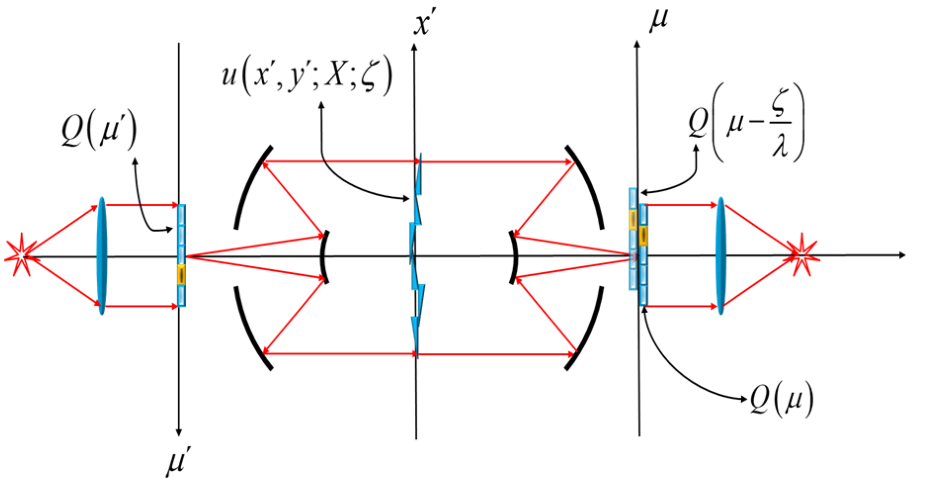
Figure 5.
Optical setup that employs two coding masks. Along the axis µ’the amplitude transmittance is Q(µ’). Along the axis µ the amplitude transmittance is Q(µ). Along the x’-axis, the object is a set of prisms. Each prism generates a deflection angle ζ, and each prism is randomly situated, at location X. In Equation (14), we indicate the amplitude transmittance of one element of the set of prisms.
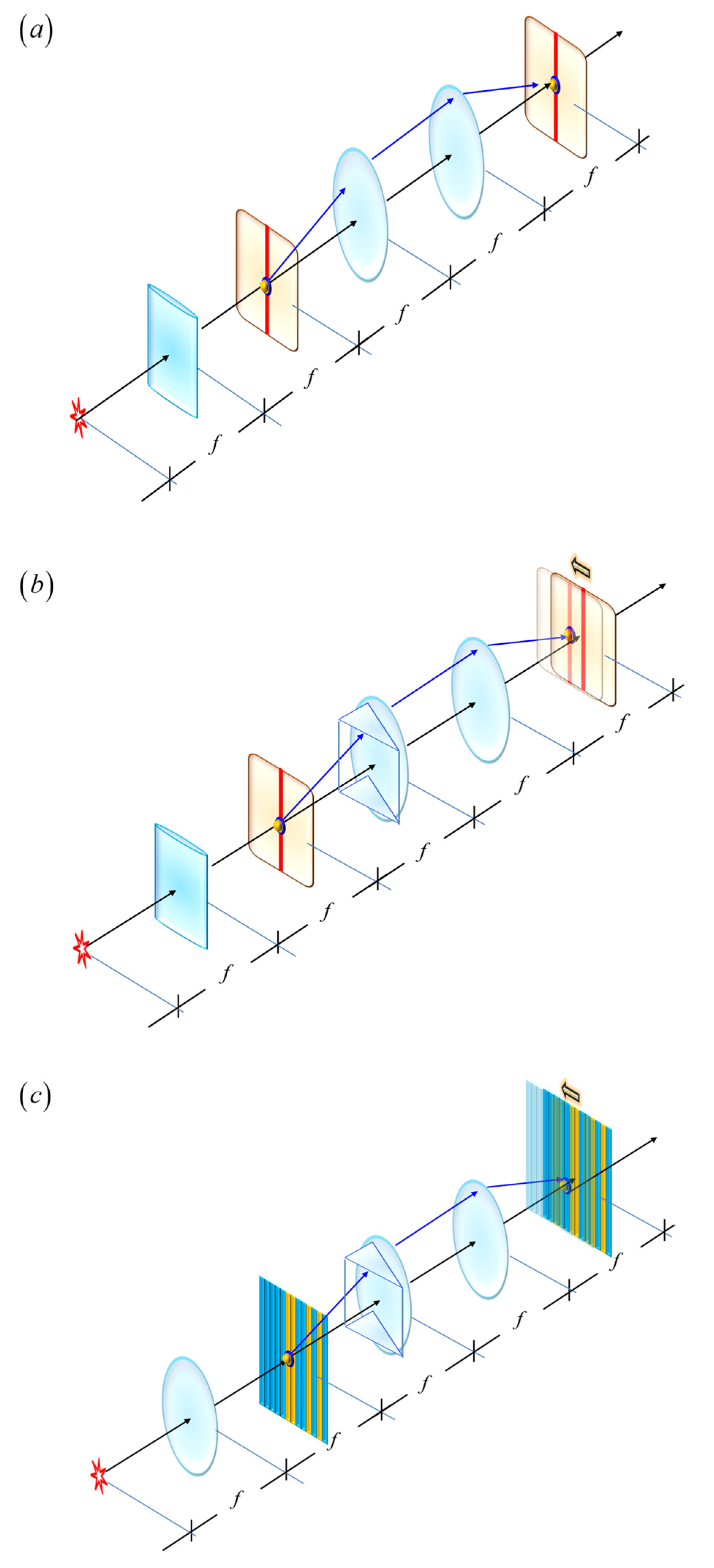
Figure 6.
Schematics depicting a coded source in conjunction with a coded spatial filter. In (a), we employ a cylindrical lens for generating a coherently illuminated slit. At its conjugate image, we employ a slit as spatial filter. In (b), we depict the impact of a phase gradient. In (c), we use a spherical lens for coherently illuminating a mask coded with a Barker sequence.
Figure 7.
Amplitude transmittance of the mask, QL (η), which is coded with a pseudorandom sequence of length L. In (a), the length is L = 7. In (b), the length is L = 15.
Figure 7.
Amplitude transmittance of the mask, QL (η), which is coded with a pseudorandom sequence of length L. In (a), the length is L = 7. In (b), the length is L = 15.
Figure 8.
Cyclic autocorrelations that are associated with the pseudorandom sequences in
Figure 7. In (
a), the length is L = 7. In (
b), the length is L = 15. The cyclic autocorrelations exhibit peaks that exceed uniform value.
Figure 8.
Cyclic autocorrelations that are associated with the pseudorandom sequences in
Figure 7. In (
a), the length is L = 7. In (
b), the length is L = 15. The cyclic autocorrelations exhibit peaks that exceed uniform value.
Figure 9.
Amplitude transmittance of the mask, QL (η), which is coded with a Barker sequence of length L. In (a), the length is L = 7. In (b), the length L = 13.
Figure 9.
Amplitude transmittance of the mask, QL (η), which is coded with a Barker sequence of length L. In (a), the length is L = 7. In (b), the length L = 13.
Figure 10.
Cyclic autocorrelation associated with the Barker sequences in
Figure 9. In (
a), the length is L = 7. In (
b), the length is L = 13.
Figure 10.
Cyclic autocorrelation associated with the Barker sequences in
Figure 9. In (
a), the length is L = 7. In (
b), the length is L = 13.
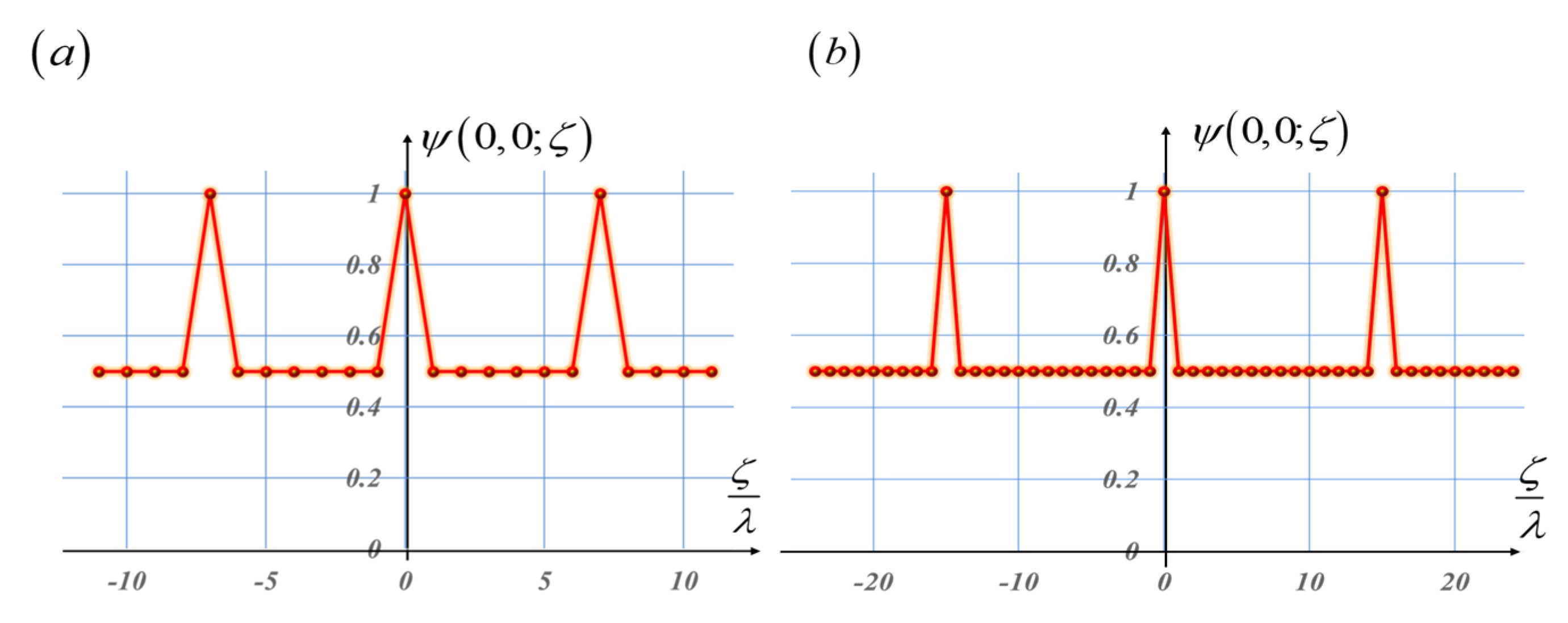
Figure 11.
The noncyclic autocorrelations have distinctive central peaks with nonuniform sidelobes. In (
a), the length is L = 7. In (
b), the length L = 15. This figure is like
Figure 7. But now, the autocorrelations are noncyclic. In this current case, the pseudo-random sequences have values that are either equal to unity, or to minus unity. The noncyclic autocorrelations have a distinctive central peak, with nonuniform sidelobes.
Figure 12.
Like
Figure 10. However, now the autocorrelations are noncyclic. In (
a), the length is L = 7. In (
b), the length L = 13. They exhibit a single central peak, with sidelobes that have constant value.
Figure 12.
Like
Figure 10. However, now the autocorrelations are noncyclic. In (
a), the length is L = 7. In (
b), the length L = 13. They exhibit a single central peak, with sidelobes that have constant value.
Figure 13.
Schematics of a Schlieren technique that acts as an automatic sensor of phase gradients. In (a), an unfolded version. In (b), a folded version.
Figure 13.
Schematics of a Schlieren technique that acts as an automatic sensor of phase gradients. In (a), an unfolded version. In (b), a folded version.
| Disclaimer/Publisher’s Note: The statements, opinions and data contained in all publications are solely those of the individual author(s) and contributor(s) and not of MDPI and/or the editor(s). MDPI and/or the editor(s) disclaim responsibility for any injury to people or property resulting from any ideas, methods, instructions or products referred to in the content. |
© 2025 by the authors. Licensee MDPI, Basel, Switzerland. This article is an open access article distributed under the terms and conditions of the Creative Commons Attribution (CC BY) license (https://creativecommons.org/licenses/by/4.0/).

