1. Introduction
Beam shaping based on diffractive optical elements enables the generation of spatial light patterns that can serve as markers for the observation of the tissue’s motion. Depending on what modality is to be observed, e.g., photoacoustics [
1], vocal fold oscillations [
2], etc., different properties of the back-scattered light should be used to evaluate the motion of the tissue. While in the case of vocal fold, 2D imaging techniques such as stroboscopy, videokymography [
3], phonovibrogram [
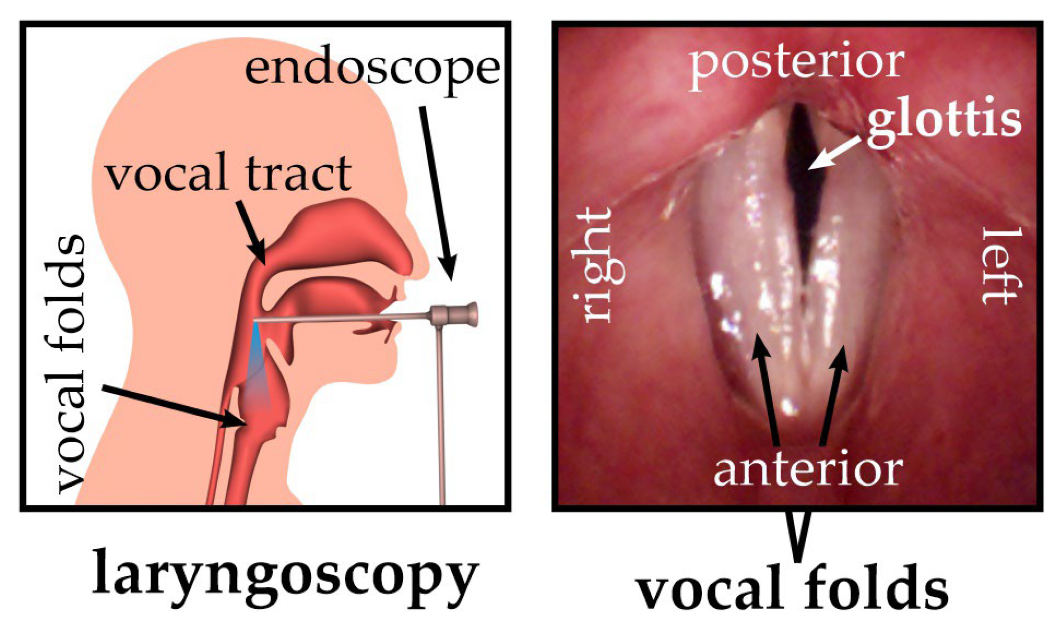
4], or high-speed videoendoscopy do not sufficiently reflect the complex 3D vocal fold dynamics (see
Figure 1), the observation of the apparent motion of the spots of a laser spot array through stereo-triangulation can be used to determine the 3D motion of the vocal folds [
5]. Early systems used individual laser points [
6,
7] or lines perpendicular to the glottal midline [
8,
9,
10], whereas later systems used regular grids for optimal coverage of the glottal plane, generated from microlens arrays [
5,
11,
12] or diffractive optical elements [
2]. This way, the vocal fold vibrations can be tracked at high frame repetition rates in both the vertical and lateral directions.
While such systems enable non-invasive in vivo observation of the vocal fold oscillations, the best results for coverage and resolution are only achieved for patients with suitable sizes of the vocal folds as well as suitable recording distances between endoscope and larynx (typically 10–15 mm VF length @ 40–70 mm recording distance in adults). For this, the divergence angle of the laser spot array and the focal plane positions of the beams need to be well chosen. Otherwise, the reconstruction of the vocal fold motion might be severely compromised as follows: (1) either by having too few points to secure sufficient coverage, (2) too large points, limiting the detection accuracy, or (3) too many points, which overlap and render the point detection impossible. In principle, this problem can be solved by commercially available dynamic diffractive optical elements [
13] as they would enable full control of, e.g., the divergence angle of the spot array, the number of beams in the array, and the focal plane position of each beam. Unfortunately, the current dynamic devices do not have the necessary small footprint to integrate them into an endoscope.
One possible solution for the above-mentioned problem is to use a static optical element to generate the spot array and then use liquid lenses to control the divergence of the spot array and the spot size by adapting the focal plane position. The versatility of liquid lenses arises from their ability to achieve large dynamic focusing ranges with rapid response times and non-mechanical actuation [
14,
15]. In electro-wetting liquid lenses, a focus variation can be induced by changing the curvature of the liquid–liquid interface between two immiscible transparent liquids with differing refractive indexes by applying a voltage via electrodes to the conductive liquid [
16]. This allows for precise adjustments within fractions of a second, making liquid lenses highly adaptable and effective, especially in many space-restricted applications. Because of this, the use of liquid lens systems plays an important role in endoscopic imaging, for beam shaping, steering, and beam delivery.
Various liquid lens-based zoom systems have been explored for compact imaging applications [
17,
18,
19]. For instance, Zhang et al. present a theoretical design and optimization of a micro zoom system employing liquid lenses for general imaging purposes [
20]. In contrast, our approach specifically targets laser spot array generation for endoscopic 3D reconstruction. Many aspects have to be considered when designing a spatially structured laser pattern for endoscopic illumination applications. This includes the device miniaturization aspects, robustness, flexibility, and patient safety. In this paper, as a proof-of-principle, we present a free-space optical system for non-mechanical beam manipulation using two liquid lenses and a static diffractive optical element (DOE). A DOE is basically a type of holographic grating that allows for a lens-free generation of arbitrary intensity patterns through diffraction; see [
21,
22,
23] for further reading. The specific DOE used here generates a laser spot array consisting of 21 × 21 individual beams and is placed between two electro-wetting liquid lenses so that the combination of the static DOE and the varioptic lenses functions as a dynamic spot array generator. The first tunable liquid lens controls the spot divergence in the final spot array, while the second liquid lens adjusts the zoom factor of the projected pattern. The system thus provides both an adjustable array size and spot size, making it particularly useful for endoscopic applications [
2]. While Semmler et al. [
2,
11,
24] provide in-depth detail of the imaging and diagnostic reasoning, this paper focuses on the specific features of the liquid lens optical design for illumination. Even though we describe our system from the viewpoint of laryngoscopy, we are positive that there are many other potential applications in the medical field, e.g., in laparoscopy [
25,
26].
2. Materials and Methods
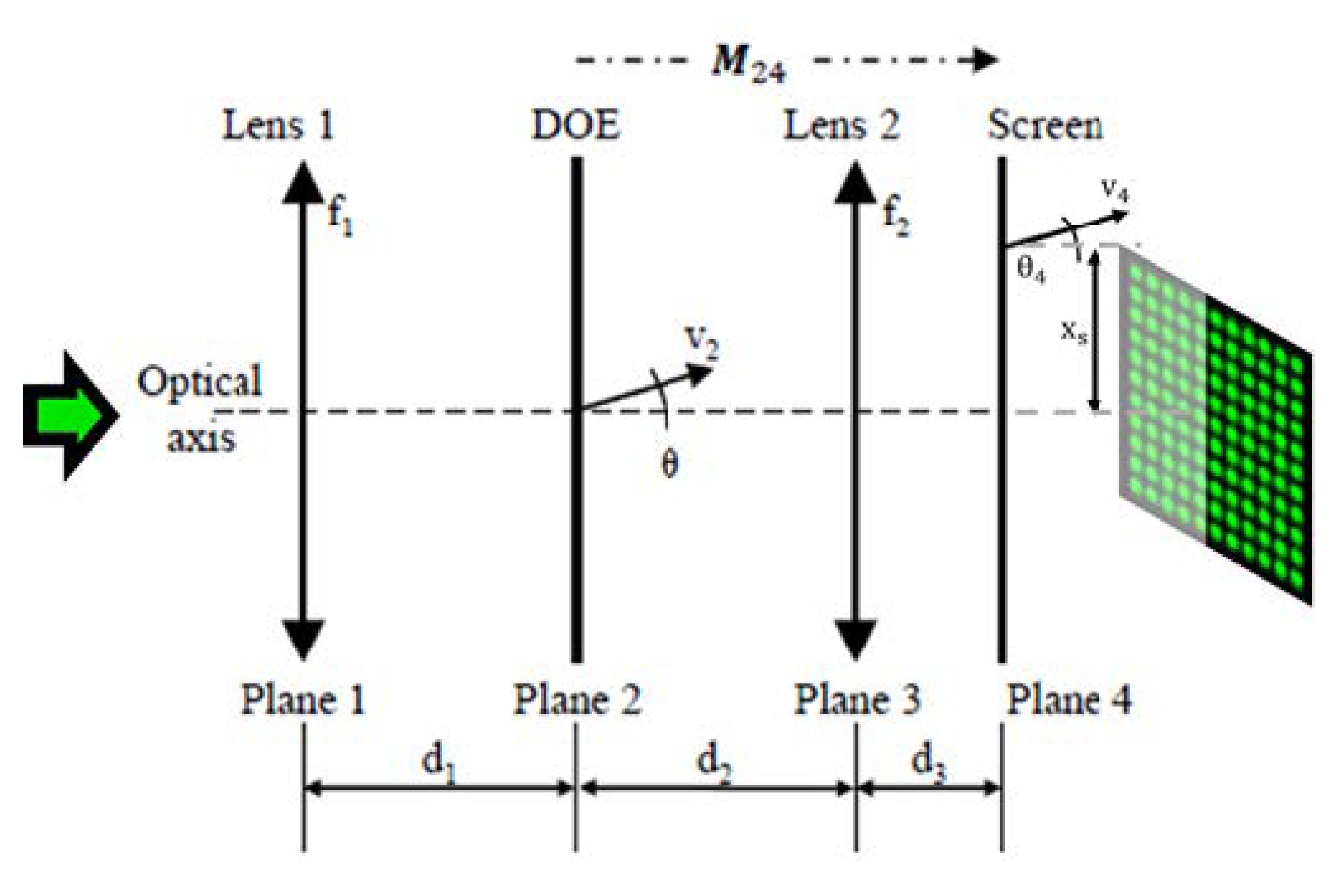
Figure 2 shows the schematic of the free-space optical setup. A diffractive optical element (DOE) custom-made from HOLOEYE is placed between two liquid lenses from Corning Inc., (New York, NY, USA), Type A-25HX-D0, whose focal lengths can be varied by adjusting the input voltage, between −35 m
−1 to +35 m
−1, with 7.75 mm outer diameter and 2.5 mm clear aperture. The DOE generates from a collimated laser beam at 532 nm a spot array of 21 × 21 beamlets of the same size and divergence as the input beam, with the 0th diffraction order suppressed down to the same intensity as the other beamlets. The divergence angle between the beamlets is 0.5°. We consider for the design of the optical system a dynamic zoom factor as follows:
We denote the physical distances between the successive optical elements as
d1,
d2, and
d3; see
Figure 2. A collimated laser beam with a beam radius of
ω1 = 179 µm is incident on the first liquid lens
L1, with the focal length
f1. The angles of the beamlets of the spot array generated by the DOE at plane 2 can be defined by the opening angle
θ between the outermost beamlet and the optical axis. The corresponding ray vector
v2, intended for the optimization of the setup via the ABCD matrix formalism (see e.g., [
27]), can be consequently defined as
v2 = {0,
θ}. Similarly,
v3 and
v4 are the ray vectors after planes 3 and 4, respectively. The liquid lens 2, with variable focal length
f2, is responsible for the zoom factor of the spot array and defines the spot array distribution at plane 4.
xs is the lateral half-width of the final intensity pattern at plane 4.
The spot array at plane 4 can be characterized in terms of the final grid size and the size of the individual spots. Both can be varied by changing the physical distances within the optical setup, as well as by adjusting the focal lengths of both the liquid lenses. In the next section, we provide the theory necessary to evaluate the operational boundaries of the tunable laser spot array generated using the given setup. An ideal dataset can be achieved by adjusting the values of d1, d2, θ, w1, f1, and f2.
2.1. Dynamic Zoom Factor
The main design objective is to maximize the dynamic zoom factor,
γ, which we define as
where max (
xs) and min (
xs) denote the maximum and minimum possible half-widths of the spot array, respectively. We note that the first lens does not affect
v2, because
v2 originates from a ray that runs on the optical axis in plane 1.
γ is thus independent of
d1 and
f1.
In order to express
γ in terms of the remaining system parameters
d2,
θ, and
f2, we set up the ray-transfer-matrix from plane 2 to plane 4 as follows:
where
L(
d) is the ray-transfer-matrix for the propagation of distance
d in air and
F(
f) is the ray-transfer-matrix for a thin lens of focal length
f. We know that
v2 is located on the optical axis and defined by the maximum beamlet deflection angle
θ given by the DOE
We can then calculate
v4:
where
will be determined by the system specifications, and as
θ is fixed by the DOE,
is dependent only on the variables
d2 and
f2, which can be chosen freely (within the boundaries of the setup and available equipment). Since we do not restrict
, Equations (5) and (6) are reduced to
and consequently,
where
and
are the focal lengths that correspond to the maximum and minimum
, respectively.
Equation (7) shows that the adjustment of the spot array size is dependent on the focal length of the second lens. Equation (8) demonstrates that
γ is independent of
θ. Hence, we are, in principle, also free to pick
θ. Equation (8) diverges for
, which corresponds to the well-known single-lens imaging condition from plane 2 to plane 4, and thus results in min (
xs) = 0 for that condition. Taking the first derivative of Equation (8) with respect to
d2, we realize that
γ increases strictly monotonously in the relevant region from
d2 = 0 mm, to the point where
d2 obeys the imaging condition. Therefore, stacking the DOE and the second lens closely together (i.e., small
d2), results in diminishing the dynamic zoom factor. Large distances (i.e., large
d2), however, require large clear apertures of the second lens, as
θ is significantly larger than zero; see
Figure 2. Picking a liquid lens component should therefore aim at a maximum clear aperture while keeping the component diameter small enough for an endoscope. Equally important, the selected component should have the largest possible dynamic adjusting range. We choose, therefore, the variable focus lens (Type A-25HX-D0) from Corning Inc. with a diopter range from −35 m
−1 to +35 m
−1 and
a3 = 2.5 mm clear aperture (7.75 mm outer diameter) over the A-16F variable focus lens with an outer diameter of 6.2 mm but only 1.6 mm free aperture [
28].
Given these constraints, we allow for
v3, a maximum aperture utilization of 66%, in order to prevent clipping for beam diameters up to 500 µm. Basic trigonometric considerations give
where
is the clear aperture in plane 3. Correspondingly,
d2 should be kept smaller than 9.4 mm. We set for our setup
.
2.2. Conservation of Étendue
Due to the conservation of Étendue [
29,
30,
31,
32], the area of illumination will change (e.g., the spot size
ω4) whenever the second lens changes the array opening angle. A smaller opening angle leads to larger spots and the spots will be spaced out on a smaller area. As a consequence, the spots will interfere for too small opening angles. In contrast, larger opening angles lead to smaller spots with a wider spacing. However, in this case, the laser fluence might increase (due to the smaller spot size) far enough to potentially lead to tissue damage and should thus be taken into account.
Since in both cases, the adjustment of the magnification factor leads to an undesired change in the spot size at plane 4, the spot size must be precompensated by the liquid lens 1 before the beamlets pass the DOE and lens 2. To determine how to adjust the focal length of lens 1 according to the magnification factor set by lens 2, we use the q-parameter method for Gaussian beams. In plane 1,
q is given by
where
z is the axial distance to the beam waist (i.e., the focal spot position),
i is the imaginary unit, and
zR1 is the Rayleigh length, given by
where
ω1 is the beam waist (radius) and
λ is the wavelength. The system is arranged such that the beam waist is located in plane 1 and hence
z1 = 0. We can prepare the transfer matrix from plane 1 to plane 4 as follows:
and calculate the beam parameter in plane 4 as
The real part of
q4 will yield
z4 and the imaginary part will yield
zR4. We can use Equation (11) and
zR4 in order to obtain
ω04, the corresponding beam waist—which is axially shifted from plane 4 by
z4. We can then calculate the actual beam radius in plane 4 using
Here,
ω4 is predefined by system requirements. As the dynamic ranges of the liquid lenses are symmetric around zero diopters, we set the incident beam radius
ω1 such that the desired beam radius in plane 4 is realized for zero refractive power applied at both lenses. Taking the successful motion tracking of the vocal fold in [
2] as a reference, we choose for our case
ω4 = 200 µm and
d3 = 75 mm. With this and
f1 =
f2 =
∞, Equation (14) gives
ω1 = 179 µm. We set this value in our experiment by placing an adjustable demagnifying telescope into the collimated 532 nm laser beam in front of the lenses shown in
Figure 2.
3. Results
For the investigation of the performance of the optical design, we recorded plane 4 on a camera sensor for five different working distances
d3, ranging from 40–70 mm, as is typical for laryngoscopy [
11]. For each working distance, we changed the liquid lens voltages such that we obtained a recording of the smallest possible spot array, one medium-sized spot array, and the largest spot array, defined by the value
xs, the half-width of the spot array size. For each of these array sizes, we also recorded the smallest possible spot size, a medium spot size, and one too large a spot size
ω4. By large spot sizes, we mean significant intensity overlap between spots.
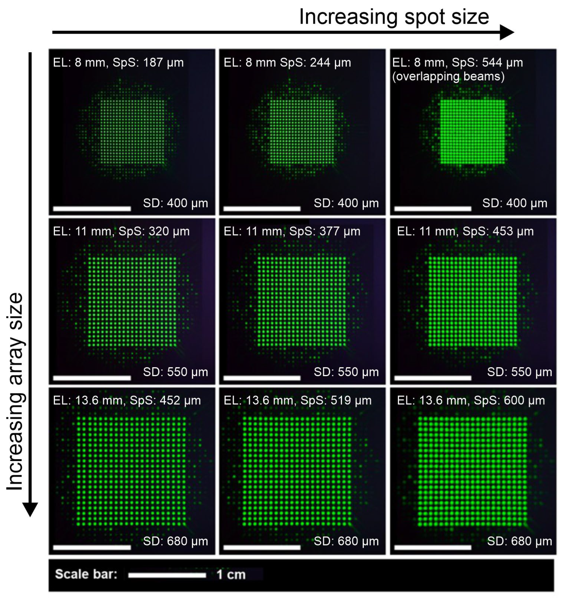
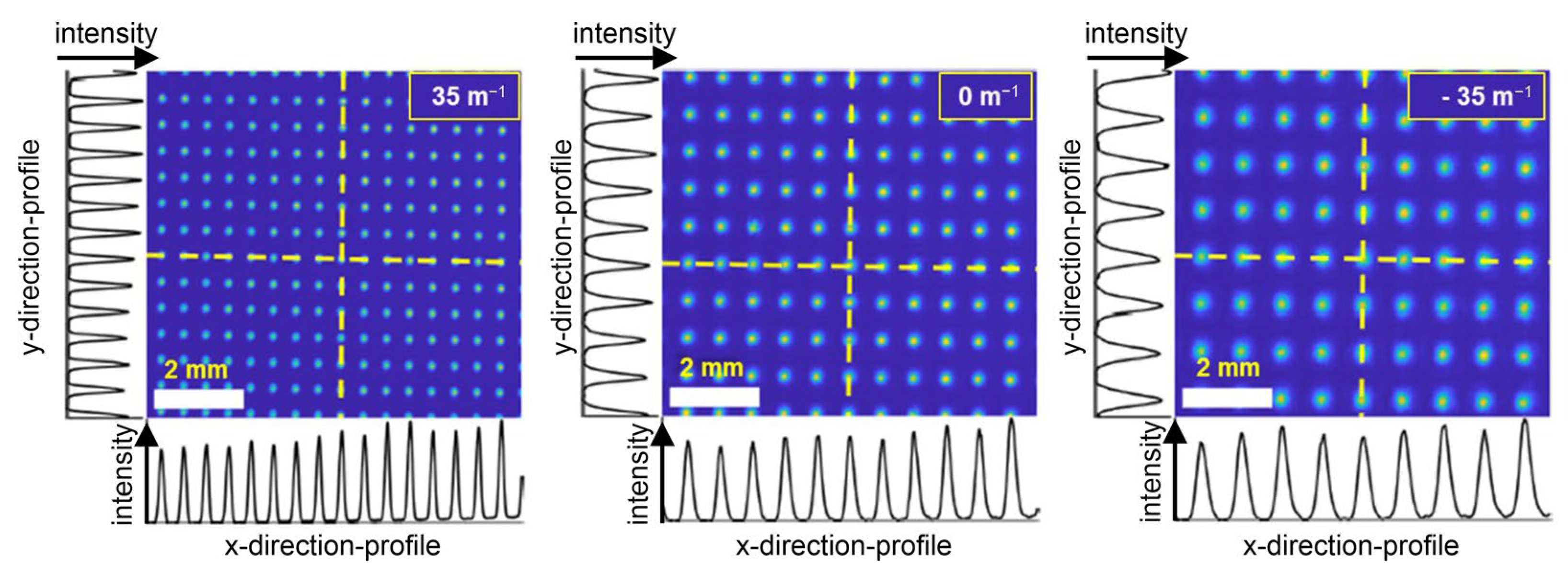
The process was conducted on two camera sensors: One was a beam profiling camera (Coherent LaserCam HR, Saxonburg, PA, USA, sensor size 8.576 mm × 6.860 mm, pixel pitch 6.7 µm) with a high dynamic range but a small image sensor, which therefore cropped the number of observable beamlets. The other sensor was a digital single lens camera sensor (a Nikon D610 camera, Tokyo, Japan, with a sensor size of 36 mm × 24 mm and a pixel pitch of 6.0 µm), with a sufficiently large area to observe all beamlets but not with the high dynamic range of the beam profiling camera. This way it was possible to investigate the action of the liquid lenses on both the spot size, spot array magnification, and any potential aberrations (see
Section 4) and uniformity deviations of all the beamlets generated by the DOE. Exemplary recordings of the beamlet array are shown in
Figure 3.
In order to accommodate the measurements for any potentially necessary hardware to encapsulate the liquid lenses, their electronic control busses as well as the DOE, we apportion 10 mm additional space behind lens 2. We thus define our working distance
zWD for future reference as
3.1. Spot Array Sizes
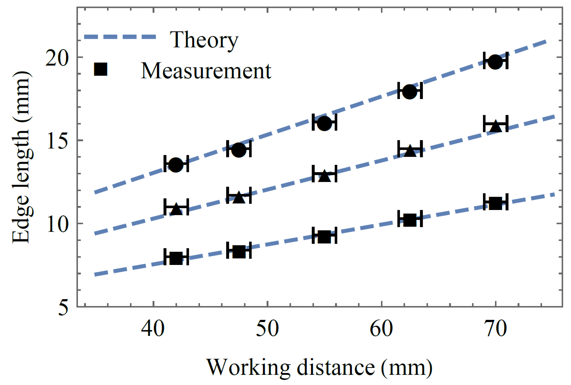
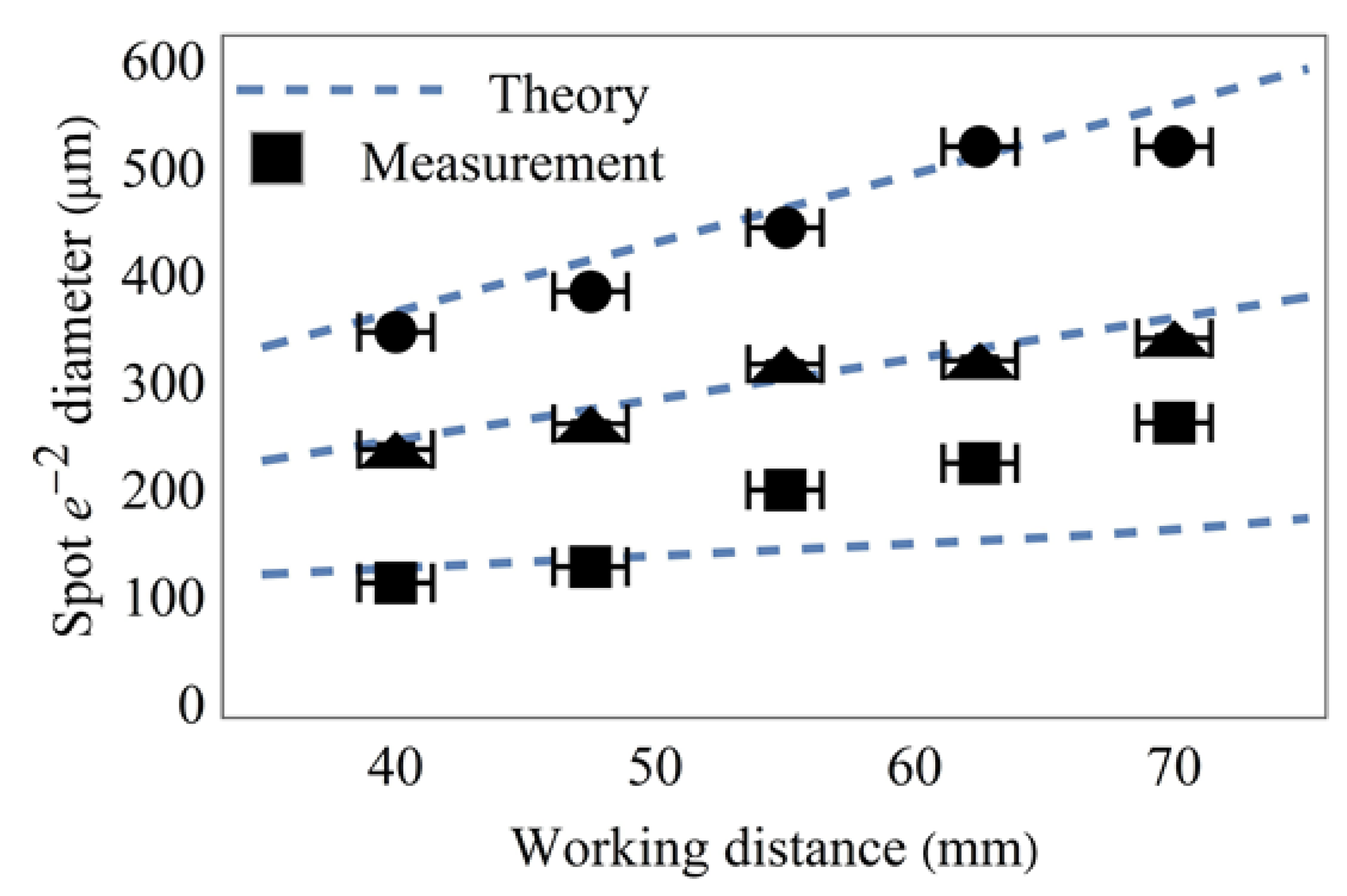
The typical working distance for laryngoscopy ranges from 40 mm to 70 mm. Due to the physical location of the camera sensor inside the housing of each of the used cameras, the smallest possible working distance was 42 mm. Therefore, we recorded at working distances of 42 mm, 47.5 mm, 55 mm, 62.5 mm, and 70 mm. In order to analyze the spot array size, we used the Nikon D610 camera (without lens or objective), set to the manual mode.
Figure 4 shows the theoretical and experimental values of the spot array size at the above-discussed working distances. Since the spot array size is dependent only on the focal length of the second lens (Equation (7)), the experiment is conducted with the refractive power of lens 1 being kept constant, while the refractive power of lens 2 is set to −35 m
−1 (circles), 0 m
−1 (triangles), and +35 m
−1 (squares). We find that the theory from
Section 2 adequately matches the measurement. In order to receive the optic design dynamic zoom factor, we divide the slope of the −35 m
−1 line (with circles) and the slope of the +35 m
−1 line (with squares) and get
γ = 1.8.
3.2. Spot Sizes at 55 mm Working Distance
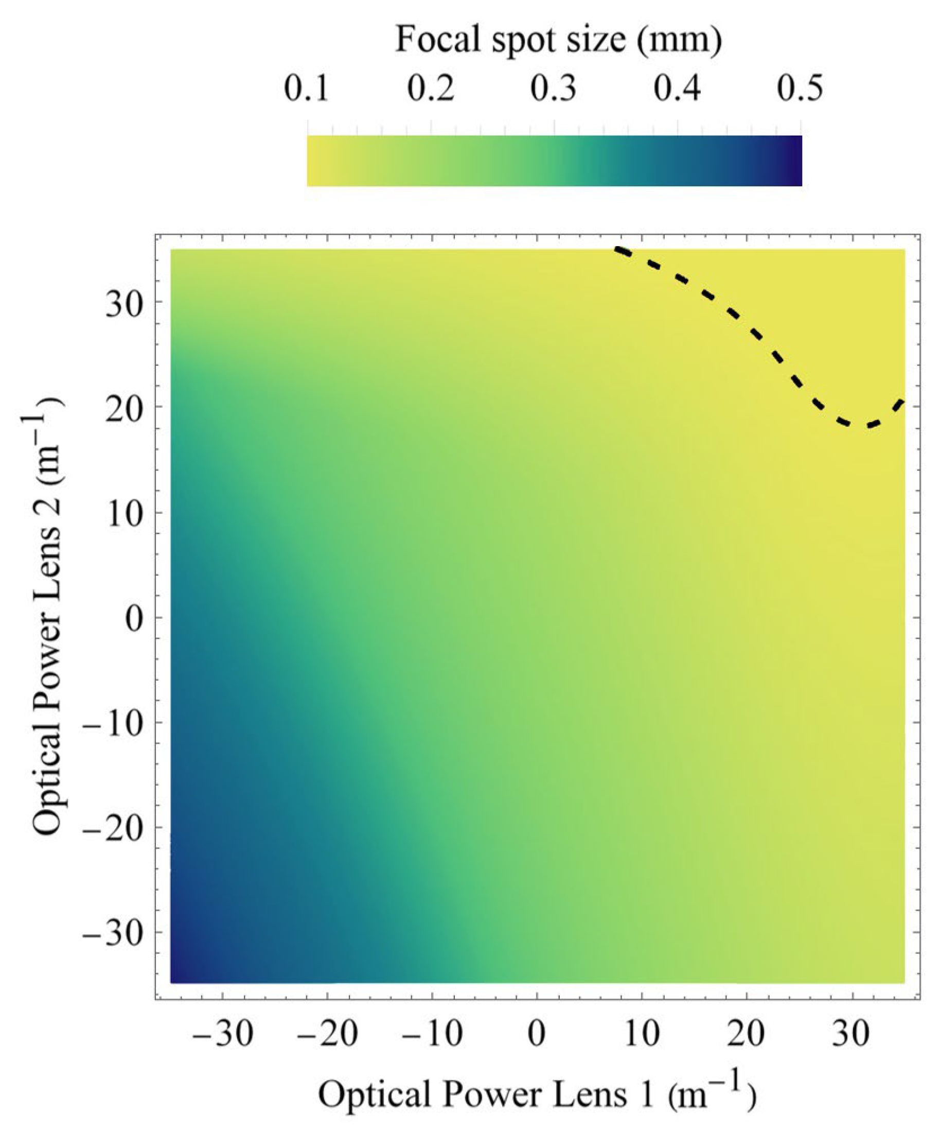
Figure 5 shows the theoretical predictions for the individual laser spot sizes as a function of the refractive powers of both liquid lenses (lens 1 and lens 2) at a working distance of 55 mm. This provides a visual representation of the entire dynamic range at this working distance. Since the array size is solely dictated by the refractive power of lens 2, a horizontal line in
Figure 5 would refer to a fixed array size. By adjusting the refractive power of lens 1, the actual working point on this horizontal line can be chosen freely, and consequently, the spot size adjusted. Spot sizes smaller than 100 µm are colored in red, and spot sizes larger than 600 µm are colored in yellow, as those cases are undesired. The colors for spot sizes between 100 µm and 600 µm are specified using the color range shown in the color bar of
Figure 5. The dashed curve indicates the contour where 100 µm waist diameter will be achieved somewhere along the beam direction; i.e., at a different working distance than 55 mm. We nevertheless plot this curve as it shows a parameter region that should be avoided at all costs due to possible laser safety issues.
The minimum possible spot sizes for each array magnification and each working distance were further investigated using the Coherent LaserCam HR. Measurement and theory are shown in
Figure 6. The spot sizes of each beamlet were calculated by fitting each spot on the camera sensor using a two-dimensional Gaussian model with rotational freedom. Taking the mean value of all fits from one recording gives the spot sizes (1
/e2 diameter) depicted in
Figure 6.
3.3. Minimum Focal Spot Sizes
Because the beamlets undergo diffraction during propagation to the tissue’s surface, the actual spot size on the tissue will not only depend on the actual chosen refractive powers of both lenses, but also on the actual distance of the tissue to the endoscope’s end; i.e., on the three-dimensional shape of the vocal fold. Since too small spot sizes are particularly critical due to possible tissue damage, the transverse beam profile outside the endoscope’s housing must be carefully evaluated. To be on the safe side, we calculate for each possible refractive power setting at lens 1 and 2 the spot size of the beam waist (i.e., the focal spot diameter) independently of how far away it might be located from the exit of the endoscope.
Figure 7 shows the beam waist diameter 2
ω04. In contrast,
Figure 5 shows the spot diameter at a working distance of 55 mm. The dashed curve indicates again the contour where the focal spot size would become 100 µm or smaller. Spot sizes smaller than this should be avoided. This is because, for the recording of the oscillations of the vocal fold, a high-speed camera (typically around 4000 fps with only 250 µs exposure duration per frame) is used that requires, due to signal-to-noise ratio (SNR) considerations, an illumination intensity while still complying with laser safety regulations [
2]. Going towards 100 µm spot diameter or below would restrict the applicable laser power, thus significantly degrading the achievable SNR of the high-speed camera.
4. Discussion
To date, all previous studies in the field of 3D imaging of the human larynx were based on a fixed geometry of the laser projection unit. There are setups with one or more laser lines as well as regular laser dot grids. There are approaches with microlens arrays or DOEs [
2,
5,
10,
11]. However, none of the previous approaches allow the laser projection to be adapted to the anatomical conditions of the subject during the recording.
As the distance from the endoscope to the larynx and the vocal fold length vary depending on the sex and age of the test subjects, in a fixed laser spot array without the proposed liquid lens design, the laser grid can only be optimized for a certain spot-to-spot distance and an average vocal fold length. Due to the necessary divergence of the laser beams between the exit window (2 mm) at the endoscope and the vocal folds in the larynx (10–20 mm), the laser points could unnecessarily hit the laryngeal tissue around the vocal folds, or conversely, the points could be so close that they overlap with each other. Compounding the problem further, the diameter of the laser spots can, in a static case, only be adjusted to lie within a certain spot size range, which means that the laser spots may be too large for exact detection. By adjusting the spot distance and spot diameter, we are able to tailor the laser grid for each larynx size so that the vocal folds are completely covered while the points can still be clearly distinguished from each other. With the achieved zoom factor of 1.8 (see
Section 3.1), the design is matched to the recording situation during human in vivo laryngoscopy, including the distance from the oral cavity to the vocal folds (40–70 mm) as well as the vocal fold length (10–20 mm).
However, just adjusting the size or edge length of the spot array by lens 2 only would lead to problems, as illustrated by
Figure 7. This is because, at higher refractive powers of lenses 1 and 2 (i.e., especially when lens 2 is used for getting shorter edge lengths of the beamlet array), there is a chance to achieve a beam spot below 100 µm, as depicted by the dashed line. This poses the risk of exceeding laser safety regulations. As this must be safeguarded against, lens 1 needs to be set to smaller diopters, even below zero, in order to increase the spot size. On the other hand, when lens 2 is used to generate large array sizes, the divergence of the beamlets increases significantly. In order to have for the high-speed camera sufficiently bright beamlets, their spot size must be smaller than their size if only lens 2 were to be involved.
Uniformity
Optical aberrations, induced by the change in refractive power of lens 2 when setting the magnification factor, could have serious effects on the visibility of individual spots and the resolution the spot array can offer. While lens 1 might also induce optical aberrations as long as the laser beam entering into lens 1 remains small enough and enters in the center along the optical axis, the aberrations should remain nearly negligible, because even for an imperfect lens, a paraxial approximation would be valid in this case. However, into lens 2, enters an already spread-out beamlet array, where the paraxial approximation might no longer be valid. Thus, refractive aberrations, such as cushion/barrel distortions, might cause a varying inter-spot distance across the spot array, while other types of aberrations, e.g., vignetting, coma, spherical aberrations, etc., might change the spot shapes and certainly decrease the available maximum intensity at aberrated spots. Therefore, they would heavily depend on the zoom factor, as the zoom factor is effectively set by controlling the curvature of the liquid in the lens.
To investigate the presence and strength of potential aberrations due to the refractive power modulation of lens 2, we measured the standard deviation of the spot-to-spot distance, the spot diameters’ standard deviation, and the standard deviation of the spot intensities depending on the refractive powers at lens 2 for different working distances. We measured at the refractive powers +35 m
−1, 0 m
−1, and −35 m
−1. All spots of a spot array using the Coherent camera sensor, shown in
Figure 8, were fitted with a two-dimensional Gaussian model, taking into account principal axis transformation. Measuring the spot positions, diameters, and amplitudes from the fit parameters, standard deviations
σ were calculated.
We chose the standard deviation because it reveals the strength of the variation in a group of measurements. The expectation is that with increasing aberrations, the standard deviation for spots of the spot array will also increase. To show only changes induced by the refractive power setting we chose to normalize the standard deviation measurements to their respective average value for all variational parameters. The graphical results are presented in
Figure 9, while the numerical results are given in
Table 1, for the sake of completeness.
As can be seen, there is no clear tendency for the standard deviations to increase when modifying the refractive power or the working distance. This is good because any clear trend would hint at the presence of optical aberrations. Furthermore, standard deviations for the spot diameter and the spot intensity seem to be rather constant, with the inter-spot distance having an exception at 47.5 mm working distance and −35 m−1 refractive power. Nevertheless, the standard deviation at this point is still only 1.2% and thus still negligible. With the standard deviations for beamlet distances below 1.2%, the beamlet’s size below 5.2%, and the beamlet’s amplitude below 10.8%, the system easily meets the requirements for three-dimensional endoscopic imaging at different working distances and magnification settings.
5. Conclusions
In this work, we introduced a dual-liquid-lens optical design that flexibly adjusts the spot size and spot distance in a laser grid generated from a static DOE. Our experiments demonstrated a dynamic zoom factor of approximately 1.8 across clinically relevant working distances and confirmed that this adaptable configuration maintains optimal coverage of the vocal folds and minimal optical aberrations. These findings establish that using tunable liquid lenses for laser-based 3D laryngoscopy can effectively address inter-patient variability, such as differing vocal fold sizes and variable laryngoscope-to-larynx distances, thereby paving the way for improved 3D reconstructions of vocal fold oscillations.
Although our proof-of-concept system has not yet been incorporated into a fully miniaturized endoscope, it serves as a conceptual foundation for future integration demonstrating the feasibility of liquid lenses in laser projection. We have shown that the combination of a static DOE with two variable focus liquid lenses offers the flexibility needed to adapt illumination parameters in real time, which is an essential step toward truly personalized and optimized laryngoscopic 3D imaging. By enabling precise control of both the laser spot array size and individual spot diameters, our approach promises to enhance reconstruction accuracy and clinical utility, and ultimately addresses many of the practical and methodological concerns surrounding next-generation endoscopic imaging systems. We anticipate that further engineering for miniaturization and control systems will facilitate the application of this design in a clinical setting, thereby offering a valuable advance over existing fixed-geometry laser projection units for endoscopy.
One issue in integrating the liquid lens principle of the current setup is the large size of the liquid lenses, as they have an outer diameter of 7.75 mm; see
Section 2. As a consequence, the placing of these lenses, and consequently the DOE, needs to occur as far as possible from the distal end of the endoscope. However, this bears the challenge of how to relay the beamlet array with its angles and beamlet divergences. One possible solution for this would be to use after lens 2, a long gradient index lens (GRIN lens) [
33] that can relay the aperture of lens 2 through 1:1 imaging of the lens’s plane. This way the spot array can be easily extended by a large margin, similar to in [
34,
35]. While commercially available GRIN lenses that offer a suitable numerical aperture to support the beamlets’ divergence angles used in the here-described setup do exist, GRIN lenses are known for inducing aberrations on abaxial beams [
36,
37]. This might lead to a non-uniform spacing of the laser spots as well as a deterioration of the spot quality at the edges. While these aberrations can be measured and precompensated in principle [
38] by using a suitably designed DOE, this is beyond the scope of this work, as we implemented a custom-designed static DOE with a regular beamlet array, which is far easier to design and manufacture. Consequently, for a miniaturization into an endoscopic setup, the interplay between the DOE and the GRIN lenses would need to be re-evaluated in greater detail.


 ,
, 


