Article

Acetone Absorption Cross-Section in the Near-Infrared of the Methyl Stretch Overtone and Application for Analysis of Human Breath

Department of Physics and Astronomy, Texas A&M University, College Station, TX 77843-4242, USA
*
Author to whom correspondence should be addressed.
Optics 2025, 6(1), 9; https://doi.org/10.3390/opt6010009
Submission received: 31 January 2025 / Revised: 26 February 2025 / Accepted: 28 February 2025 / Published: 12 March 2025

Abstract

:
We present an empirical model for the cross-section of low concentration acetone gas in the range of 1671.5–1675 nm that encompasses the absorption band of the methyl stretch overtone. This model is experimentally validated with cavity ring-down spectroscopy (CRDS) measurements performed with a calibration gas and its diluted mixtures with breath samples. Particular attention is paid to accurate wavelength measurements with an interferometric wavemeter. The theoretical framework for analysis of gas mixtures with several absorbing species is presented. We show that the proposed empirical model can be used to accurately determine the concentration of acetone vapor in human breath samples. The comparison of the acetone absorption cross-section with previous results is also presented.

1. Introduction

Spectroscopic detection of acetone is a task that arises in several fields. In the medical domain, it has attracted significant interest due to the potential of acetone as a biomarker for diseases like type-1 diabetes (T1D) and possibly type-2 diabetes (T2D) [1], and heart failure [2,3]. It can also be used for monitoring patients with ketoacidosis [1,4] and those on a ketogenic diet rich with fats [5]. Typical concentrations of acetone in exhaled breath of healthy individuals are from 0.2 ppm to 1.03 ppm, which for T1D patients can be elevated to 1.7–3.8 ppm and even higher [1]. The concentration of acetone in atmospheric air normally is much lower, within 1–10 ppb [6,7], which requires even more sensitive techniques for environmental monitoring. The need for spectroscopic analysis of acetone also appears in astronomical observations [8,9].
Multiple spectroscopic techniques have been employed to accurately detect volatile organic compounds (VOCs) in air and exhaled breath: cavity ring-down spectroscopy (CRDS) [10,11,12], tunable diode laser absorption spectroscopy (TDLAS) [13], wavelength modulation spectroscopy (WMS) [14,15], frequency comb laser absorption spectroscopy (FC-LAS) [16], and the results are summarized in recent reviews [17,18,19]. Another sensitive technique that can be used for detection of VOCs is photoacoustic spectroscopy (PAS) [20,21].
Besides spectroscopic approaches, other sensitive techniques such as gas chromatography-mass spectrometry (GC-MS), proton transfer reaction mass spectrometry (PTR-MS), and selected ion flow tube mass spectrometry (SHIFT-MS) have been used for breath analysis, and some references and results with these techniques can be found in review papers [1,17]. The main advantages of the NIR-CRDS approach presented here are its relative simplicity, low cost, and small footprint, combined with sufficiently high sensitivity and specificity.
For the detection of acetone, electronic transitions in the UV region [22,23] as well as vibrational absorption bands in the near-infrared (NIR) and mid-infrared (MIR) spectral regions were employed. In the UV range, the attenuation due to scattering starts prevailing over the absorption coefficient of acetone when it reaches the value of 2 × 10 6 cm−1 [18]. The reflectivity of the mirrors limited at this wavelength by about R = 0.993 also reduces the sensitivity limit to about 10 6 cm−1 [18], which at practical pressures does not make it possible to reach the required sensitivity level of portions of ppm.
In the MIR, several fundamental vibrational modes of acetone are located, which offer strong absorption cross-sections and ultimately a very high sensitivity can be realized with quantum cascade lasers. With WMS near 3367 nm, detection limits as low as 0.12 ppm with 60 s signal averaging time were achieved [15], and with PAS near 8270 nm, the detection limit of 0.25 ppb with the lock-in integration time 10 s was reported [20]. However, compared to NIR, laser sources and detectors in the MIR range are more expensive, and the noise level at room temperature is relatively high, which requires cooling of the detector. For CRDS, the achievable reflectivity of the mirrors in the MIR are typically substantially lower than what is possible in the NIR. Even with the cross-sections in the NIR about 100 times smaller than in the MIR, still NIR CRDS provides sufficient sensitivity for detection of acetone in exhaled breath.
The absorption cross-sections for acetone in the MIR were determined in the 830–1950 cm−1 (5.128–12.05 μ m) spectral range using a high-resolution FTIR spectrometer [24]. In the NIR, the absorption cross-section of the C–H overtone was determined for isoprene, 1,3-butadiene, and 2,3-dimethyl-1,3-butadiene [23], using continuous wave cavity ring-down spectroscopy (CW-CRDS) and known absorption cross-sections in the UV region. Results on the absorption cross-sections of acetone in the NIR region are scarce, especially measurements performed in a gas mixture. Some previously obtained results are presented in the discussion in Section 5.
In this work, we perform measurements of the absorption cross-section of acetone for the overtone of the C-H stretching mode in the spectral range of 1671.5–1675 nm. For this purpose, NIR-CRDS was used. The technique leverages an optical cavity with highly reflective mirrors, causing light to circulate multiple times through the sample. This extended path length enhances the interaction between the light and the sample, making it possible to detect trace amounts of acetone and other accompanying gases. The high sensitivity of NIR-CRDS allows for detection limits down to the level of tens of ppb, which is sufficient for measurements of breath samples.
NIR-CRDS offers several advantages compared to other spectroscopic techniques. It can target specific overtones and combination bands in the near-infrared region since the laser sources in this spectral range are readily available. The NIR-CRDS setup is relatively simple and can be used in applications such as medical diagnostics or environmental monitoring. Since the technique measures the decay rate of light rather than absolute absorption intensity, it can perform with minimal interference from environmental noise or fluctuations in laser power unlike some other absorption techniques where the light intensity must be carefully monitored for accurate concentration results. The selected wavelength interval provides the advantage of only minor interference of the absorption lines of water vapor and CO2, which are significantly present in human breath and the atmosphere. NIR-CRDS benefits from the long effective path lengths created by the highly reflective mirrors in the optical cavity. In fact, an interaction length as long as 137 km was reached in our setup.
In the NIR, acetone has a relatively broad absorption band which peaks at a wavelength of 1672.44 nm [25]. The broadband absorption can be seen in the main plot of Figure 1, while the inset shows a zoom of the peak absorption feature. This feature shown in the inset of Figure 1 is particularly interesting because it can be measured with the tuning range of a typical DFB diode laser, and it is this feature that we aim to characterize. The shape and magnitude of this absorption feature of acetone have been measured for pure gas samples and those diluted with laboratory air at low pressure. However, it has yet to be verified if there are distortions in the spectrum shape occurring in the presence of other gas species at breath concentrations and at higher pressures.
In this investigation, we show that the absorption cross-section of acetone in the range of 1671.5–1675 nm has a consistent shape that is independent of pressure in the range of 30–500 Torr and is not affected by the high concentrations of water vapor present in human breath. Additionally, we characterize this absorption feature by providing an empirical formula for the cross-section valid to high accuracy, which we demonstrate is useful for providing an accurate determination of acetone concentration in human breath samples. The developed NIR CRDS setup, despite its simplicity, is robust and efficient in performing breath analysis in the desired sensitivity range down to tens of ppb level for acetone.

2. Theoretical Basis

2.1. Description of Spectral Measurement with CRDS

The method of CW-CRDS [27] allows for calibration-free measurement of the absorption coefficient of weakly absorbing species present in the mode volume of a high finesse optical cavity. The presence of this absorbing species modifies the finesse of the optical cavity, and this change can be sensitively observed through the ring-down time of the cavity [28].
The ring-down time of the optical cavity is measured with CW-CRDS by coupling laser light into the cavity and rapidly shutting off this laser with an external modulator. The light intensity, which is transmitted through one of the cavity mirrors, can then be observed to undergo and exponential decay, which is well modeled by the function
y ( t ) = A e t / τ + B
where τ is the ring-down time, and A, B are two fitting constants.
In the absence of any absorbing species, the optical cavity will have some baseline ring-down time which, in terms of the speed of light c and the round-trip length of the cavity L, is
τ 0 ( λ ) = L / c 1 R 2 ( λ ) + X
which is in general dependent on wavelength. Here, R ( λ ) is the wavelength-dependent reflectivity of the cavity mirrors, which we assume is the same for both mirrors. Additional losses in the cavity (diffraction and scattering) are taken into account by the X term. This baseline can be measured by evacuating the chamber which houses the optical cavity to remove any gaseous species.
In the presence of a species having absorption coefficient α which is weakly absorbing ( α L < < 1 ), the ring-down time is given for a two-mirror cavity of round-trip length L by [28]
τ ( λ ) = L / c 1 R 2 ( λ ) + X + α ( λ ) L
In the limit of small absorptions ( L / c τ < < 1 ), the absorption coefficient can be extracted in a calibration-free manner by the use of
α ( λ ) = 1 c 1 τ ( λ ) 1 τ 0 ( λ )
By scanning the laser wavelength over the interval of interest, we obtain a measurement of the absorption spectrum α ( λ ) . Since the quantities (2) and (3) cannot be measured simultaneously for the optical cavity, we must conduct two separate scans of the baseline and filled chamber. To evaluate τ 0 ( λ ) at some wavelength, we evaluate the straight line fit to the baseline measurement. Our experimental results show that this is a valid approximation for the behavior of the baseline. The behavior of the baseline is fairly stable as long as the cavity mirrors are not contaminated.

2.2. Retrieving Concentrations from Absorption Measurements: Analysis of a Gas Mixture

For a gas mixture having m different absorbing species with mole fractions y j (which we will refer to as concentrations) and absorption cross-sections σ j ( λ ) , we can write the absorption coefficient as
α ( λ ) = P k b T y 1 σ 1 ( λ ) + y 2 σ 2 ( λ ) + + y m σ m ( λ )
In general, the cross-sections σ j depend on the presence of other gas species [29] and the temperature T and pressure P of the mixture [30].
σ j ( λ ) = σ j ( λ ; T , P , y 1 , , y m )
We give the analytic solutions for the concentrations y j in Equations (8) and (A29) which are computed under the assumption that the cross-sections do not depend explicitly on y i . For the gas species measured in this work, which are cataloged in the HITRAN database [30], only very small corrections [29] to the lineshape functions are known to be arising from the interaction with other gas species. The NIR absorption of acetone is not well cataloged in the HITRAN database, but it was also found in Section 4.1 that the acetone cross-section displayed neither pressure dependence nor distortion in the presence of other species. Therefore, we maintain the assumption that the cross-sections do not depend on y j .
In the case where the cross-section has explicit dependence on y j , iteration can be used. Using an initial guess for y j to compute the cross-section, the analytic solution of either (8) or (A29) is used to compute a new set of concentrations which can then be used to update the cross-section σ j ( λ ; T , P , y 1 , , y m ) . By iterating this process only a few times, a solution is obtained which includes the effect of other gas species on the cross-section. For the rest of this work, we will only consider cross-sections which have dependence on the total temperature and pressure σ j ( λ ) = σ j ( λ ; T , P ) .
For a measured spectrum consisting of N values of the absorption coefficient α i at wavelength λ i , we have for m different absorbing species having each cross-sections σ j
α 1 α 2 α 3 α N = P k B T σ 1 ( λ 1 ) σ 2 ( λ 1 ) σ m ( λ 1 ) σ 1 ( λ 2 ) σ 2 ( λ 2 ) σ m ( λ 2 ) σ 1 ( λ 3 ) σ 2 ( λ 3 ) σ m ( λ 3 ) σ 1 ( λ N ) σ 2 ( λ N ) σ m ( λ N ) y 1 y 2 y m
Here, α i = ( 1 / τ i 1 / τ 0 ) / c is the absorption coefficient determined from the measured ring down time τ i conducted at wavelength λ i . We denote the N by m matrix in Equation (7) as A, the length N column vector on the left as α , and the length m vector on the right as y . For N > m , the over-determined system (7) can then be written as α = A y , and the least squares solution is given by
y = ( A T A ) 1 A T α
The above expression gives values of the concentrations y i which provide the best fit to the data after they have been converted to absorption. This simple analytic solution can be written since α model is linear in the gas concentrations y j . The use of the weighting function can give reduced squared deviation from the data to the fitting curve in spaces other than absorption, as described in Appendix B. We also show in Appendix C that the weighting function can improve the estimates for the concentrations recovered from the spectrum fitting. It is possible to account for baseline instability by the inclusion of additional terms in the fitting model such as the α B ( λ ) models described and analyzed in Appendix C.

3. Experimental Setup and Methods

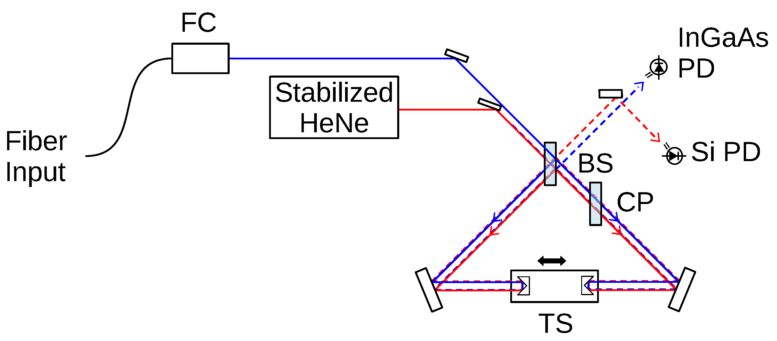
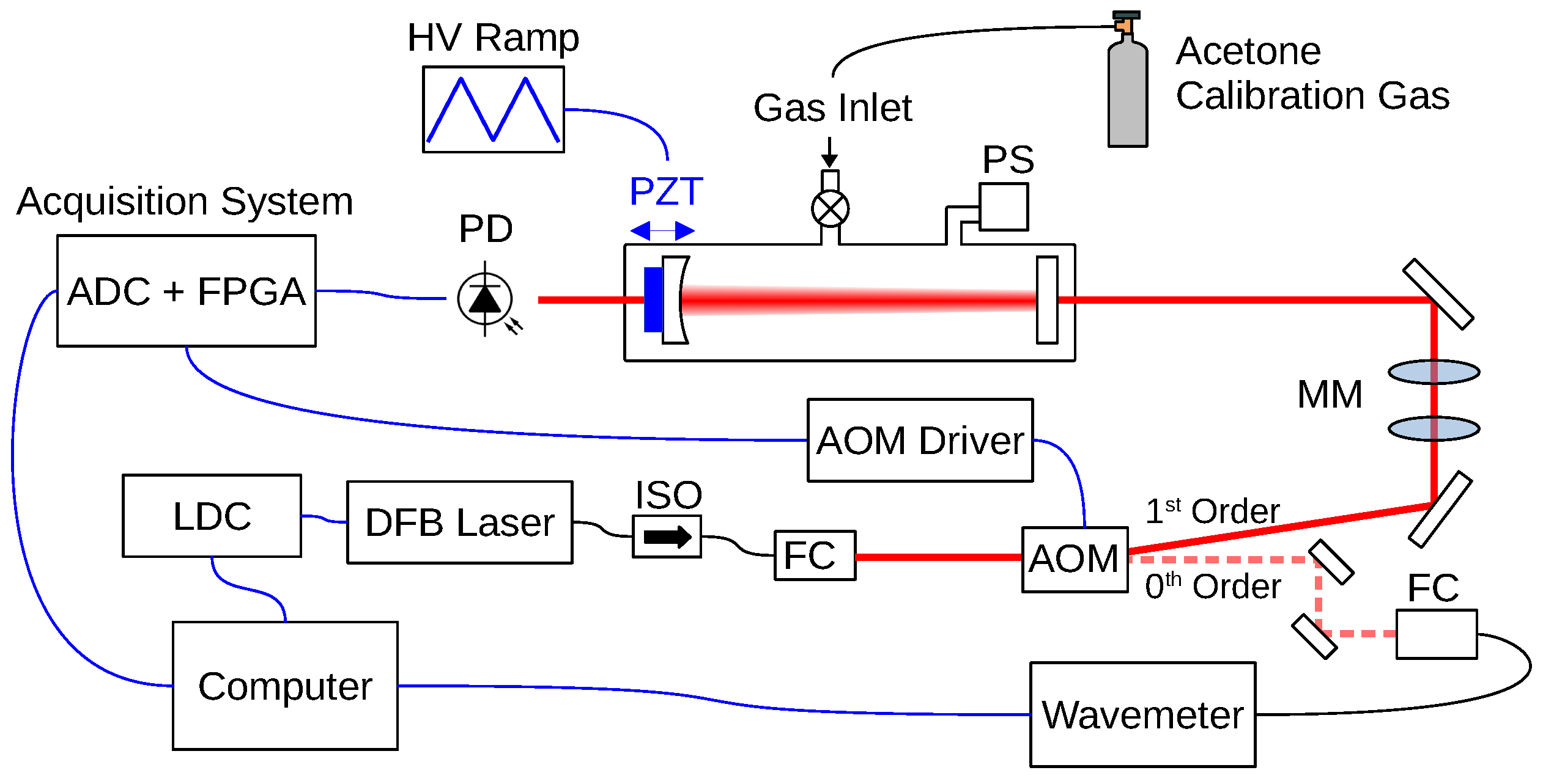
3.1. Experimental Apparatus

The schematic of the experimental setup is shown in Figure 2. The laser source is a commercially available distributed feedback diode laser (DFB) (Eblana Photonics EP1673-7-DM-B01-FM). It is available as a 14-pin butterfly package. The output of this fiber pigtailed laser is fed through a fiber-coupled isolator (ISO) and then collimated using a fiber collimator (FC) package. In order to use this CW laser source, it was necessary to employ a fast optical modulator [27]. This is accomplished by using the first diffraction order output of an acousto-optic modulator (AOM) operated in the Bragg regime, as this allows for a high extinction ratio and fast switch-off times of the first-order deflected beam. The optical high finesse optical cavity is of hemispherical type, consisting of a planar and concave high reflectivity mirrors separated by a distance of 1.72 m. The input coupler is a flat mirror, and the output coupler has a concave shape with 2 m radius of curvature. The output coupler is mounted to a ring-shaped piezoelectric transducer (PZT), which slightly alters the length of the cavity. The output beam passes through the middle of the PZT, out of the chamber using a wedged AR-coated window, and is focused onto an amplified photodiode (Thorlabs PDA10CS) with an off-axis parabolic mirror.
The first-order deflected beam is mode-matched to the optical cavity with a mode matching telescope consisting of two planoconvex lenses. The alignment and mode-matching of the cavity were verified by eliminating the presence of higher-order transverse modes. These could be seen by sweeping the length of the cavity using the PZT and monitoring the cavity transmission using the photodiode.
The cavity resonance excitation is performed by applying a high voltage triangular wave (shown as HV ramp) to the PZT, which modulates the optical frequency of the cavity resonances. The amplitude of the triangle wave is chosen such that a single cavity resonance always sweeps over the frequency of the laser. Also shown is the laser diode controller (LDC) and GPIB connection to the computer. The acquisition system consists of a single board computer (Red Pitaya STEMlab 125-14, Solkan, Slovenia) which has onboard 14-bit analog-to-digital converter (ADC) and a field-programmable gate array (FPGA), which is used to provide a low-latency switching signal to the AOM driver, allowing the laser to shutoff when resonant excitation of the cavity is detected on the photodiode (PD) by a rapid signal rise to a pre-defined threshold. This single board computer also performs the fitting of the exponentially decaying signal of the transmitted through the cavity light with the model Equation (1). The amplitude term A captures variations in the coupling between the laser and cavity.
The analog ring-down signal is processed using a low-noise pre-amplifier (Stanford Research Systems SR560, Sunnyvale, CA, USA) which features a 1 MHz single-pole low-pass filter. This signal is acquired at 125 MHz sampling rate by the acquisition system, which is down-sampled to 125/64 MHz. Additional digital filtering is performed by the FPGA prior to down-sampling in order to reduce noise aliased to low frequency [31]. The down-sampled signal is stored in the RAM of the single-board computer and passed to the operating system, which is then fit using an optimized fitting routine written in C. The initial portion of the recording is trimmed to remove the cavity buildup and corresponding transients [31].
The signal is recorded using 4000 data points and the fit is conducted with 20 iterations of the Levenberg–Marquardt algorithm. This fitting is performed on the same single board computer which performs the measurement to avoid additional latency from transferring the analog trace. An initial guess of the parameters is calculated using the Fourier transform method of [32] using the FPGA of the acquisition system to perform the Fourier integrals in real time.
From the fit of the model Equation (1) to the recorded signal, we obtain the measured cavity ring-down time τ . The amplitude term A captures variations in the coupling between the laser and cavity. The B term allows for the small offset that is output by the photodetector electronics.
For precise control of the gas mixture measured by the cavity ring-down technique, the optical cavity is constructed inside of a vacuum chamber. The pressure of the chamber is monitored by a pressure sensor (PS). Two separate pressure transducers are used; one is a diaphragm-type pressure gauge (Vacuum Research 902321, Pittsburgh, PA, USA), providing a measure of the total pressure inside the chamber which is independent of gas composition. The other is a thermocouple gauge (Varian 531) used to verify that a pressure of < 10 3 Torr is obtained when evacuating the chamber using a fore-pump (Leybold, Scrollvac SC15D, Cologne, Germany).
The ring-down time of the cavity, which is in general wavelength-dependent, gives a sensitive measure of the intracavity losses including the contribution from absorbing gas species present between the cavity mirrors. The zero-order beam emerging from the AOM is coupled into a single mode fiber and sent to the wavemeter, which is described in the next section.

3.2. Scan of the Wavelength

The laser wavelength is tuned by changing the temperature and injection current of the laser diode, both of which are controlled by GPIB communication between the computer and the laser diode controller (LDC in Figure 2). Fine control of the laser wavelength is established by adjusting the laser diode injection current. The laser current is stabilized within 25 ppm with a resolution of 0.01 mA using a Newport LCM-39420 module in an LDC-3900 laser diode controller. For course wavelength adjustment, the temperature of the diode is actively stabilized by the LCM-39420 module. The set point of this stabilization can be adjusted to a precision of 0.1 °C.
The scan of the laser wavelength is conducted by first scanning the laser current from 110.00 to 109.00 mA. After finishing the scan of laser current, the temperature is changed by 0.2 °C and the current scan is reset. This scan order is preferred to minimize the frequency of temperature changes of the laser diode since there is a longer time required for the laser to settle into a stable wavelength with temperature variations compared to changes in the current.
At each point in the scan, the AOM trigger is disabled and the wavelength is measured from the zero-order output beam of the AOM. This is achieved by fiber coupling this beam and then sending the output of the fiber to a home-made precision wavemeter (Appendix A). The AOM trigger is disabled so that the intensity changes caused by the AOM on the zero-order beam do not affect the wavelength measurement. The AOM creates a small shift equal to our driving frequency of 80 MHz between the zero- and first-order AOM beams. This discrepancy is much smaller than any of the spectrum features in this investigation and we will not be concerned with it.

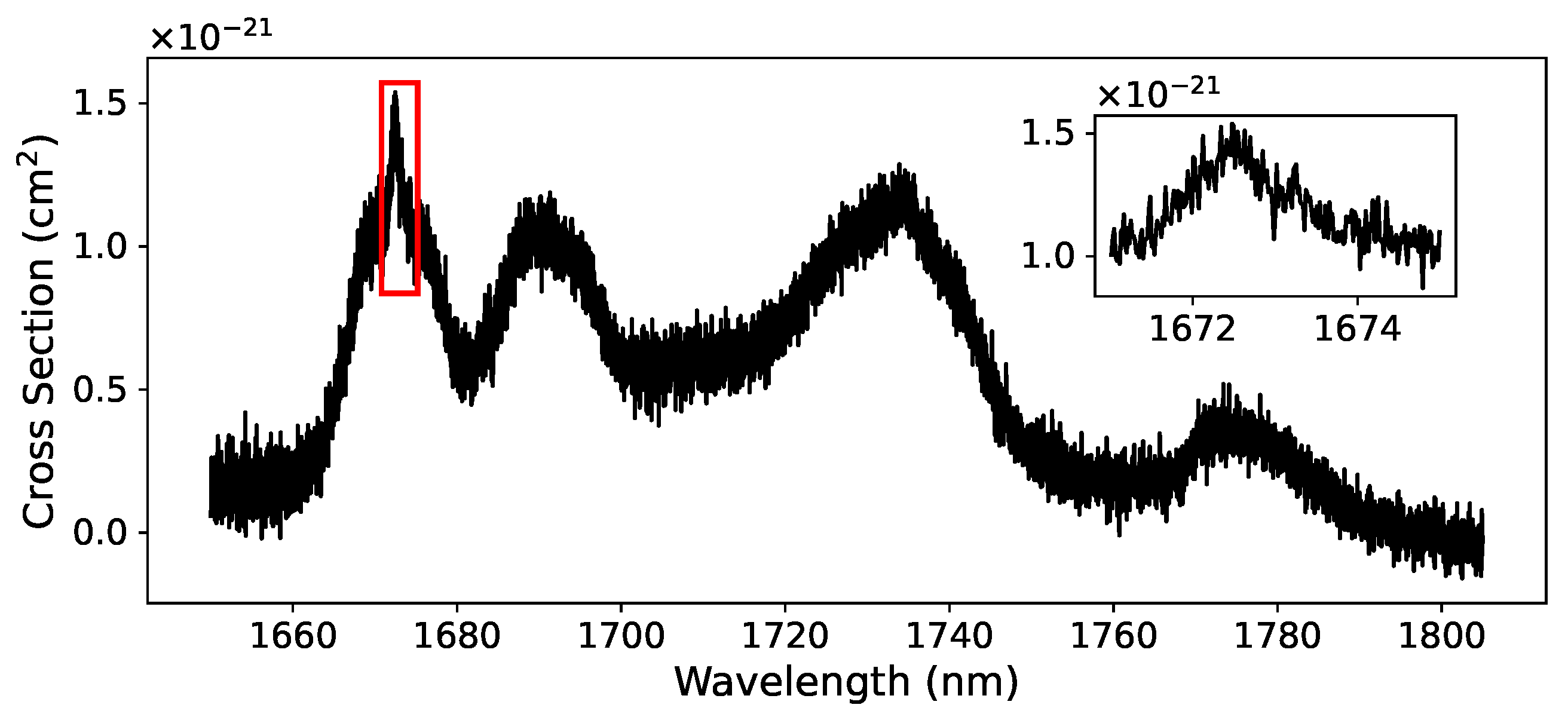
3.3. Acetone NIR Absorption Characterization

Calibrated gas mixtures of acetone were obtained from GasCo at 5 ppm and 30 ppm. The calibration of the mixtures are NIST-traceable, and the calibration certificates of the mixtures claim 10.02 ppm ± 2% and 27.33 ppm ± 5%, respectively. We investigate the shape of the NIR absorption spectrum of acetone by measuring the sample of 27.33 ppm calibration gas under various pressures and conditions of dilution, including conditions of human breath samples.
The chamber was first evacuated and the baseline ring-down time measured. A linear fit of the baseline ring-down time against wavelength is later used to evaluate τ 0 ( λ ) when the absorption is calculated from (4). The evacuated chamber was filled with an initial pressure measured on the diaphragm gauge, and the wavelength dependent ring-down time of the cavity was determined by taking the average of 100 separate ring-down measurements conducted at 1000 different wavelengths. The duration of the scans was in the range of 1–2 h, with spectra containing larger absorptions taking longer due to the decreased light being transmitted from the cavity.
The calibration gas was first measured with minimal dilution to establish that the acetone absorption cross-section does not show any detectable pressure dependence in the range of 30–141 Torr. Using the same sample of calibration gas, we also investigated the acetone absorption in the range of 141–500 Torr by diluting with ambient air. No distortions of the acetone cross-section were detectable at these increased pressures.
During this investigation, it was found that the amount of time spent vacuuming the chamber had an effect on the long-term stability of the acetone absorption measurement. This effect is investigated in more detail in Section 4.2. In light of this drift, an optimized procedure was used to minimize the effect and to report the parameters for the acetone cross-section in Section 4.3.
In Section 4.4, we demonstrate the utility of the acetone cross-section model by measuring the acetone concentration in samples of human breath. We further demonstrate the accuracy of this process by diluting these samples with a known amount of calibration gas and showing that the subsequently measured spectrum is consistent with the amount of acetone gas added and the initial measurement.
The ring-down time measurement noise is characterized in Section 4.5, and this information is used in Appendix C to simulate the effect of this noise on the spectrum fitting process and quantify the error which is propagated to the final gas concentration determination.

4. Results

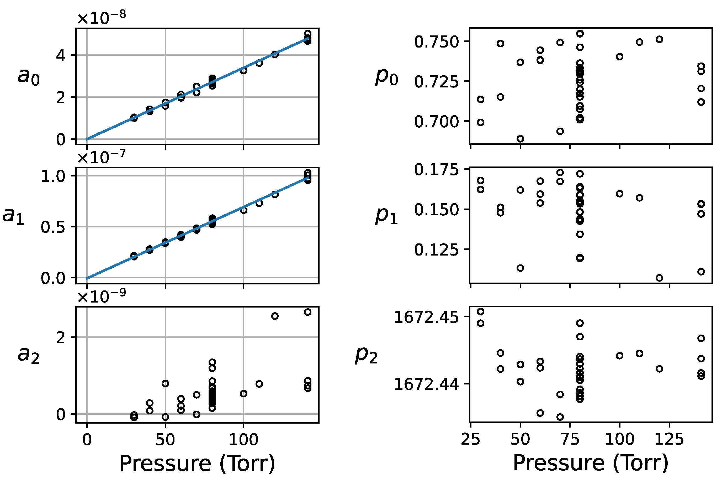
4.1. Pressure Dependence of the NIR Acetone Absorption

Cavity ring-down spectroscopy provides an absolute measurement of the absorption coefficient α [28], which is defined as the absorption cross-section σ times the number density of molecules n,
α ( λ ) = n σ ( λ )
The cross-section can, in general, be dependent on the pressure, temperature, and presence of other gas species. The linearity of the acetone NIR absorption with number density has been established for pure acetone samples in [33] from 2 × 10 3 to 9 × 10 2 Torr, indicating that the NIR cross-section for acetone must, to some degree, be independent of pressure. In this paper, we extend the range of conditions under which the NIR absorption of acetone is known to be linear.
We monitored the broadband shape of the NIR acetone absorption feature in the range of 1671.5–1675 nm by constructing an empirical model of the peak shape. We give a normalized peak shape σ ˜ ac in the form
σ ˜ ac ( λ ) = Γ 2 ( λ p 2 ) ( λ p 2 ) 2 + Γ 2 ( λ p 2 )
where the width parameter Γ ( λ ) is given by a linear dependence on wavelength
Γ ( λ ) = p 0 + p 1 λ
The p 1 term characterizes the asymmetry of the peak, and for p 1 = 0 the above function reduces to a symmetric Lorentzian peak. We scale σ ˜ ac ( λ ) to an amplitude c 0 and offset by a constant c 1 to give the model acetone cross-section
σ ac ( λ ) = c 0 σ ˜ ac ( λ ) + c 1
The peak of this model cross-section occurs at λ = p 2 with a magnitude c 0 + c 1 .
The proposed shape of the NIR acetone absorption cross-section (12) fits well with the experimental data in the wavelength range of this investigation, but results in difficulties when this function must be extrapolated to fit extended wavelength ranges in future investigations.The peak shape function σ ˜ ac ( λ ) approaches a constant at large values of λ p 2 and has a zero at Γ ( λ p 2 ) = 0 . To amend this, the function Γ ( λ ) can be clamped such that a linear behavior is displayed in this wavelength range but then rolls off to a constant value outside of it before encountering the zero of Γ . These considerations could be used to construct a modified model which extrapolates well.
To model the experimentally observed spectra, we include the effect of water vapor contamination and an imperfect absorption baseline. The calibration gas mixtures used for this measurement were not perfectly pure and contained some additional absorption primarily due to water vapor. This contamination was small in comparison to the desorption of water from the aluminum chamber walls. Due to limitations of the chamber construction, the setup could not be heated to remove this outgassing. It was therefore necessary to separate the contributions from acetone and water vapor absorptions. The need for baseline corrections results from the drift which is discussed in Section 4.2.
In order to fit the experimentally measured spectra of the calibration gas at different pressure values, the following model is used:
α ( λ ) = a 0 σ ˜ ac ( λ ) + a 1 + a 2 ( λ λ 0 ) + a 3 σ H 2 O ( λ )
The a 0 , 1 are related to the c 0 , 1 cross-section parameters by the ideal gas number density P / k B T and the concentration of acetone y ace , and similarly, the a 3 is related to the concentration of water vapor y 3 by
a 0 , 1 = y ace P k B T c 0 , 1 a 3 = P k B T y 3
The a 2 term is included to reduce the effect of drift which tends to tilt the observed spectra when the acetone absorption is slightly drifting. This was necessary for some of the calibration gas measurements since a long-term drift in the acetone absorption was observed (see Section 4.2). The use of this term corresponds to the B = 1 fitting model discussed in Appendix C, and offers improved immunity to spectrum tilt at the expense of degraded a 0 , 1 determination. It was also found that the use of the a 2 baseline slope parameter introduced a slight amount of crosstalk with the p 1 parameter and hence was not used in the final determination of the cross-section parameters. The λ 0 parameter does not affect the final expanded form of the baseline polynomial a 1 + a 2 ( λ λ 0 ) , but choosing λ 0 = 1673.5 nm in the center of the scan reduced correlation between a 1 and a 2 .
The absorption cross-section of water σ H 2 O ( λ ) was calculated using the HAPI Python module [34], which can simulate the absorption cross-sections of many atmospheric molecules using parameters in the HITRAN database [30]. For these calculations, measurements of the total chamber pressure and temperature are needed. The broadening parameters were initially calculated under the assumption of a dry air mixture, with this assumption iteratively relaxed (Section 2.2).
The fit of the model was performed using Levenberg–Marquardt algorithm to vary the nonlinear model parameters p 0 , p 1 , p 2 , and the wavelength correction factor p λ from Equation (A2). For each trial value of these parameters, the linear coefficients a 0 3 of the model absorption were determined using the unweighted linear decomposition procedure (8).
The fit of Equation (13) to the observed absorption spectrum yields the concentration of water vapor from the values of a 3 using the relation of Equation (14) and the relative contributions of the offset term a 1 and the peak amplitude a 0 . The baseline slope term a 2 includes the contribution from a tilt of the spectrum which was attributed to the long-term drift (see Section 4.2) occurring during the course of the acquisition.
The p 0 2 define the shape of the acetone absorption, and changes in these values are indicative of a changing cross-section. In this investigation, we confirmed that the values of p 0 2 stayed relatively constant and the values of a 0 and a 1 were linear with acetone number density over a range of 30–500 Torr, indicating that the cross-section showed no dependence on pressure. Additionally, we confirmed this behavior in the presence of laboratory air in the range of 141–500 Torr.

Absorption Linearity in the Range of 30–500 Torr

For pressures in the range of 30–141 Torr, we investigated the absorption pressure dependence of a sample of dry air mixture 27.33 ppm calibration gas. The sample was used as provided from the supplier, preventing dilution by flushing the gas lines several times and evacuating the measurement chamber before filling. The linear behavior of the absorption magnitude is seen from a 0 , 1 when plotted against pressure, indicating that there is very little effect of pressure and self-broadening on the absorption cross-section.
Shown in Figure 3 are two sequences of acetone calibration gas measurements along with their fits to the model absorption of Equation (13). The pressure was changed by partially evacuating the chamber using the scroll pump. For the measurements shown, the chamber was filled at 120 Torr and 50 Torr. A slight upward tilt of the measured absorption spectrum can be seen on the larger wavelength side of these two measurements, which was later attributed to a long-term drift of the acetone absorption (Section 4.2). The narrow absorptions of water can be seen superposed on the acetone absorption. The values of the coefficients obtained from the fit to the absorption curve are shown as by the points of Figure 4 plotted against pressure.
Very little distortion of the peak shape was revealed by the near constant values of p 0 and p 2 resulting from the fitting, as seen in Figure 4. The relatively large variance of p 1 is attributed to a coupling with the a 2 baseline slope term. Due to the presence of drift, we could not remove the interfering term without detrimentally affecting the fit. Because of this, we did not use the data presented in Figure 4 for the final resolution of the coefficients p 0 2 . This is discussed further in Section 4.3. Additionally, this drift resulted in poor control of the calibrated mixture, so we did not use the slope of the fit line (as was done in [33]) to resolve the final value for the cross-section magnitude.
In the range of pressures 141–500 Torr, we further investigated the linearity of the absorption by diluting the same sample of acetone calibration gas using ambient laboratory air in several increments. In this case, diluting the sample does not appreciably change the number density n, but only changes the pressure of the measurement environment and introduces contaminants. We therefore expect the absorption magnitudes a 0 and a 1 of the resulting fit to remain approximately constant as the dilution is performed for a linear absorption.
Indeed, a 0 and a 1 did not show any effect of the dilution and only showed a long-term dependence which is shown in the left panel of Figure 5 and resembles the long-term drift behavior further investigated in Section 4.2. A similar drift behavior can be seen in Figure 6a. With the exception of a few outliers, the values for p 0 2 shown in the right panel of Figure 5 showed stable behavior, indicating that the shape of the acetone peak was unchanging.
The only indication that there is some distortion of the peak shape can be seen in the bottom left of Figure 5, where there is a slight fluctuation of a 0 / a 1 . This ratio characterizes the height of the acetone absorption peak to the local offset and is independent of acetone concentration in our model. We attribute this small variation over time to contaminants which result in an apparent broadband and featureless absorption that increases the value of a 0 in the fit. This could result from increased scattering as an increasing amount of atmospheric gas is let into the chamber.

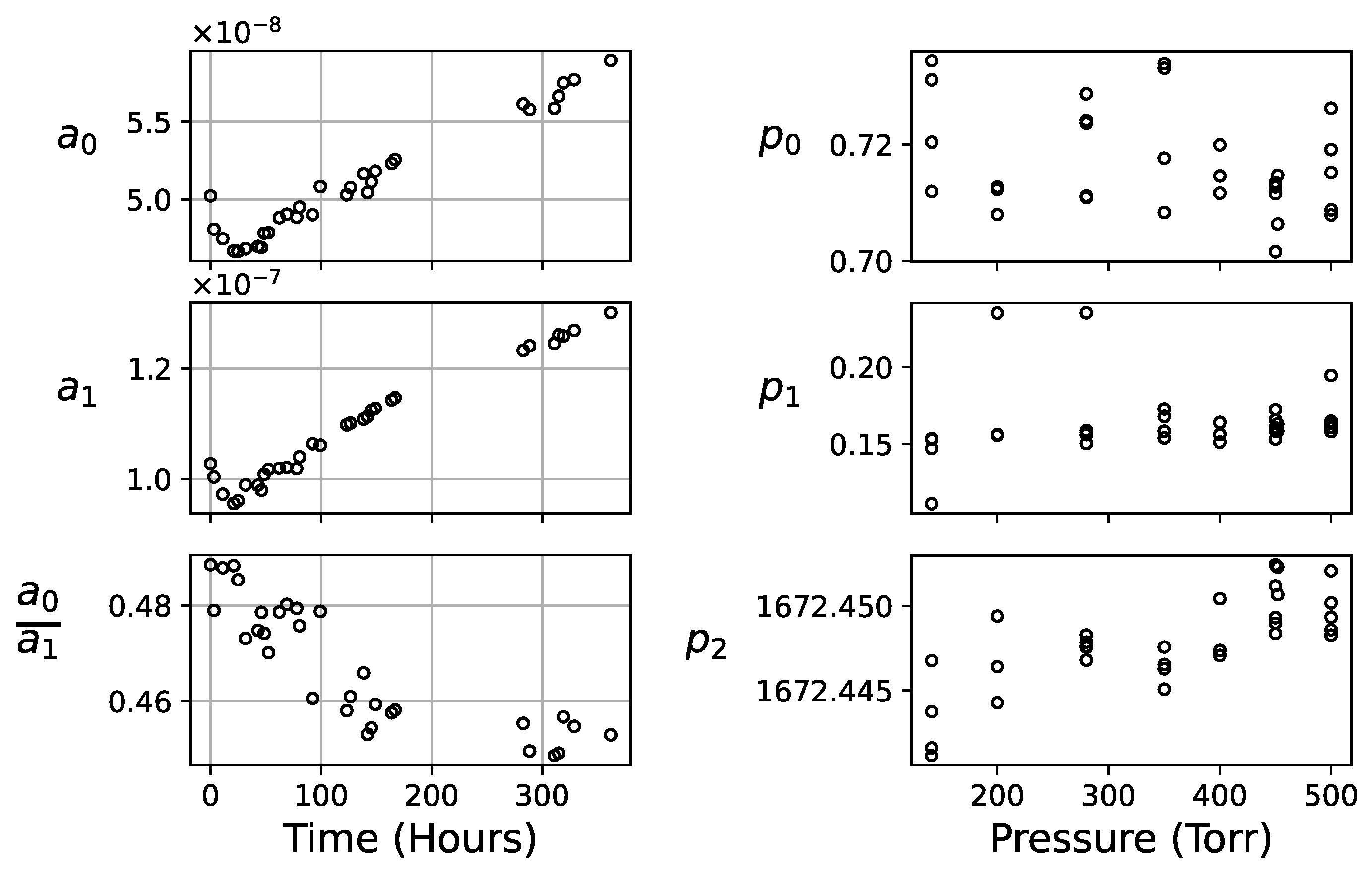
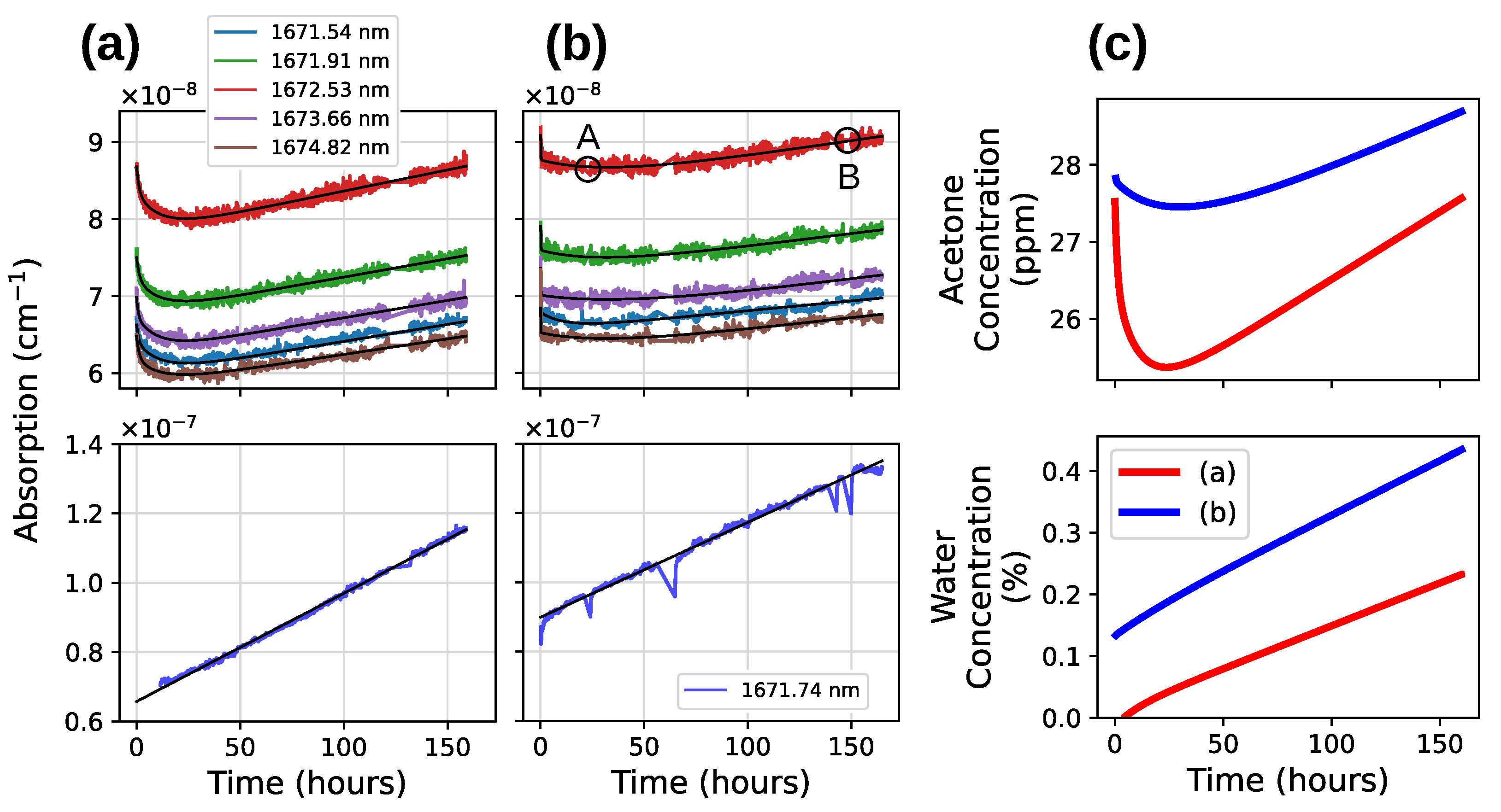
4.2. Drift of the Acetone Absorption

It was determined that the main limiting factor in our spectrum measurements was the apparent drift of the acetone absorption over a span of many hours. Since scans of the spectrum took a period of 1–2, h this drift was accounted for by using the a 2 slope term in the fit Equation (13). Coupling of this term with the p 1 resulted in a degraded ability to resolve the value of this coefficient.
To quantify the nature of the spectrum drift, we choose five wavelengths which reside on the acetone feature between the sharp water features, and a sixth wavelength was chosen to monitor an isolated water peak. The results of two different long-term drift measurements is shown in Figure 6. It was found that the time dependence of these absorption values was well modeled by a double exponential function plus a linear term
α ( t ) = m t + b + A 1 e t / T 1 + A 2 e t / T 2
In Figure 6, two different drift measurements are shown in panes (a) and (b) and compared in pane (c). The preparation of the sample was nearly identical in both cases except for the amount of time spent by the chamber under low vacuum prior to acetone calibration gas introduction. In (a), the chamber had been continuously pumped for six hours after the thermocouple gauge had reached its minimum reading of 0.001 Torr, and in (b) the chamber was only pumped down to 0.1 Torr. A much greater defect between the initial absorption value and that obtained roughly 20 h later is observed in the conditions of (a). It should be noted that the values of peak acetone absorption obtained in other studies agree most closely with this initial absorption value. In light of this finding, we decided to conduct the measurements for the coefficients in Table 1 under the conditions of (b), where the defect is smallest.
For each wavelength in the drift measurement, we fit a curve to the absorption coefficient over time using Equation (15). The water absorption was fit using a simple linear equation. The fit equations are shown as black curves in panes (a) and (b) of Figure 6. The evaluation of these curves was used to check for distortions of the acetone absorption profile.
We additionally used the model drift Equation (15) to evaluate five different absorption values from which a fit of p 1 , a 0 , and a 1 was obtained. This was done to eliminate the considerable time required for the laser to fully stabilize to a new wavelength, as evaluating the temporal fit equation allows us to know the absorption at several wavelengths simultaneously. To recover the shape of the acetone absorption, p 0 and p 2 were held fixed and a 2 was held at zero. This three-parameter model was used to fit to the five different acetone probe points to monitor for changes of the peak shape during the time evolution of the spectrum. It was found that the value of p 1 extracted from these fits then became stable and all of the spectrum evolution was contained in a 0 and a 1 , which seemed to vary together keeping the ratio a 0 / a 1 nearly constant. This indicates that the acetone absorption evolved as a scale factor, and the drift is most likely due to a changing number density of acetone, and not a distortion of the NIR peak.
Under the assumption that the change in the acetone absorption profile is due to a changing acetone concentration, Figure 6c was constructed from the measurements shown in panes (a) and (b). For a set of chosen times in the measurement interval, the fit equations to the changing absorption were evaluated to yield six absorption measurements at six known wavelengths. These were used to set up the system of Equation (7) to be established from which the concentrations of acetone and water vapor could be solved using (8). By repeating this procedure for many selected times in the measurement interval, we construct the curves shown in Figure 6c.
From Figure 6c, we see that, in the first 20 h, the drift is much more severe for the case wherein the chamber walls were dried with vacuum desiccation prior to sample introduction. Due to the long time scale, we attribute the drift to an interaction of acetone with the aluminum walls of the chamber, but this requires further investigation. The chamber in our case was rather large, having the shape of a rectangular prism of approximate internal dimensions 9 × 13 × 76 cm.

4.3. Determination of Model Coefficients

Determination of the cross-section coefficients was performed by fitting the model
α ( λ ) = a 0 σ ˜ ac ( λ ) + a 1 + a 2 σ H 2 O ( λ )
to the absorption measurements conducted at the relatively stable laboratory temperature of 21.8 °C, as measured by an AccuRite Iris weather station located in the laboratory. It was found that the slope term contained in (13) was not necessary for achieving a good fit to the data when the drift was minimized. The above model gave improved stability of the p 1 coefficient contained in the σ ˜ ac term and is equivalent to the B = 0 model simulated in Appendix C. The resulting fit parameters allow the offset a 1 and peak amplitude a 0 to be determined independently, which correspond to c 0 , 1 through (14).
In determining the values in Table 1, care was taken to evaluate only spectra which had been taken in the minimum of the temporal variation observed in Figure 6. This point is marked by the black circle marked A in pane (b). At this point, the tilt of the spectrum induced by the drift of the acetone absorption is minimized and we can uniquely determine the spectrum shape. Additionally, we analyzed data collected in the linear portions of the drift with the wavelength scan conducted in a back-and-forth motion, allowing the relatively slow drift to make roughly equal and opposite contributions across the scan. Such a point is marked B in Figure 6b.
The shape of the spectrum was not found to show any dependence on pressure or the presence of other species under the conditions that were investigated. Since the coefficients of this model resulting from the fitting procedure gave stable values, we simply took an average of the results to report the numbers in Table 1.
Table 1. Values of the coefficients resulting from the fit of the acetone cross-section at T = 21.8 °C. The peak of the model acetone cross-section is given by a 0 + a 1 1.22 ± 0.01 cm 2 .
CoefficientValueUncertaintyUnit
c 0 3.92 × 10 22 0.05 × 10 22 cm 2
c 1 8.3 × 10 22 0.1 × 10 22 cm 2
p 0 0.704 0.002nm
p 1 0.174 0.002unitless
p 2 1672.442 0.001 nm

4.4. Measurements with Diluted Breath Samples and Breath Dilution Procedure

We demonstrate that the concentration of acetone can be recovered from the NIR spectrum of a breath sample using the acetone model cross-section (12) with coefficient values from Table 1. We first measure the absorption spectrum of a breath sample, dilute this sample with a known amount of acetone calibration gas, and then measure the absorption spectrum again. If the concentration of acetone is accurately recovered from the two breath samples, then the concentrations obtained from the two spectra should be consistent with the known dilution.
A pressure around 70 Torr was found to be the optimum to measure breath samples in our apparatus in this wavelength range. A higher sample pressure would cause the water peaks to saturate the measurement such that τ 0 , resulting in the cavity producing nearly zero transmission signal. Operating just before this point allows for the highest signal-to-noise ratio of the observed signal while still fully capturing the large water absorptions.
We first filled the chamber (after the baseline τ 0 ( λ ) is characterized) with a breath sample to 70 Torr and measured the spectrum. The cavity was then partially evacuated to 65 Torr and then diluted with calibration gas to the original pressure of 70 Torr. To transfer the breath sample to the measurement chamber, the volunteer is asked to fill a latex balloon, which is then temporarily sealed with a binder clip. This balloon is placed in a refrigerator for approximately 15 min to quickly reduce the temperature of the sample. This is done to prevent condensation on the inside of the chamber and gas lines, since fresh breath gas is warmer than the 21.8 °C laboratory environment. The final transfer to the evacuated measurement chamber was performed by attaching the balloon to a 1″ KF connector and opening a needle valve in a controlled manner to avoid disturbing the optics. The chamber filling rate can be monitored with high sensitivity by monitoring the positions of the cavity resonances in the scan of the PZT (shown in Figure 2), since the refractive index of the gas changes monotonically with pressure. The final filling pressure is determined using the diaphragm gauge.
The measurements of both the diluted and un-diluted spectra were conducted at 1000 different wavelengths with 100 averages each. This number of averages is smaller than the optimum (see Section 4.5) but this smaller number of averages enabled a faster scan, limiting the effect of the drift mentioned in Section 4.2. This smaller number of averages also places our measurement in the regime of Gaussian white noise (the linear portion of the Allan plot in Figure 8b), which enables a more direct comparison with the simulation results of Appendix C.
The concentrations of the various gas species recovered from the fitting procedure are shown in Table 2 for the sample shown in Figure 7 before and after the dilution. The calibration gas used for the dilution was measured to contain only a trace amount <0.01 ppm of methane and <100 ppm water. The pre-dilution concentrations recovered from the fit are used to compute the expected concentrations resulting from a dilution with pure acetone calibration gas and these are shown in the fourth column of Table 2 and compared to the values resulting from the spectrum fit of the diluted gas.

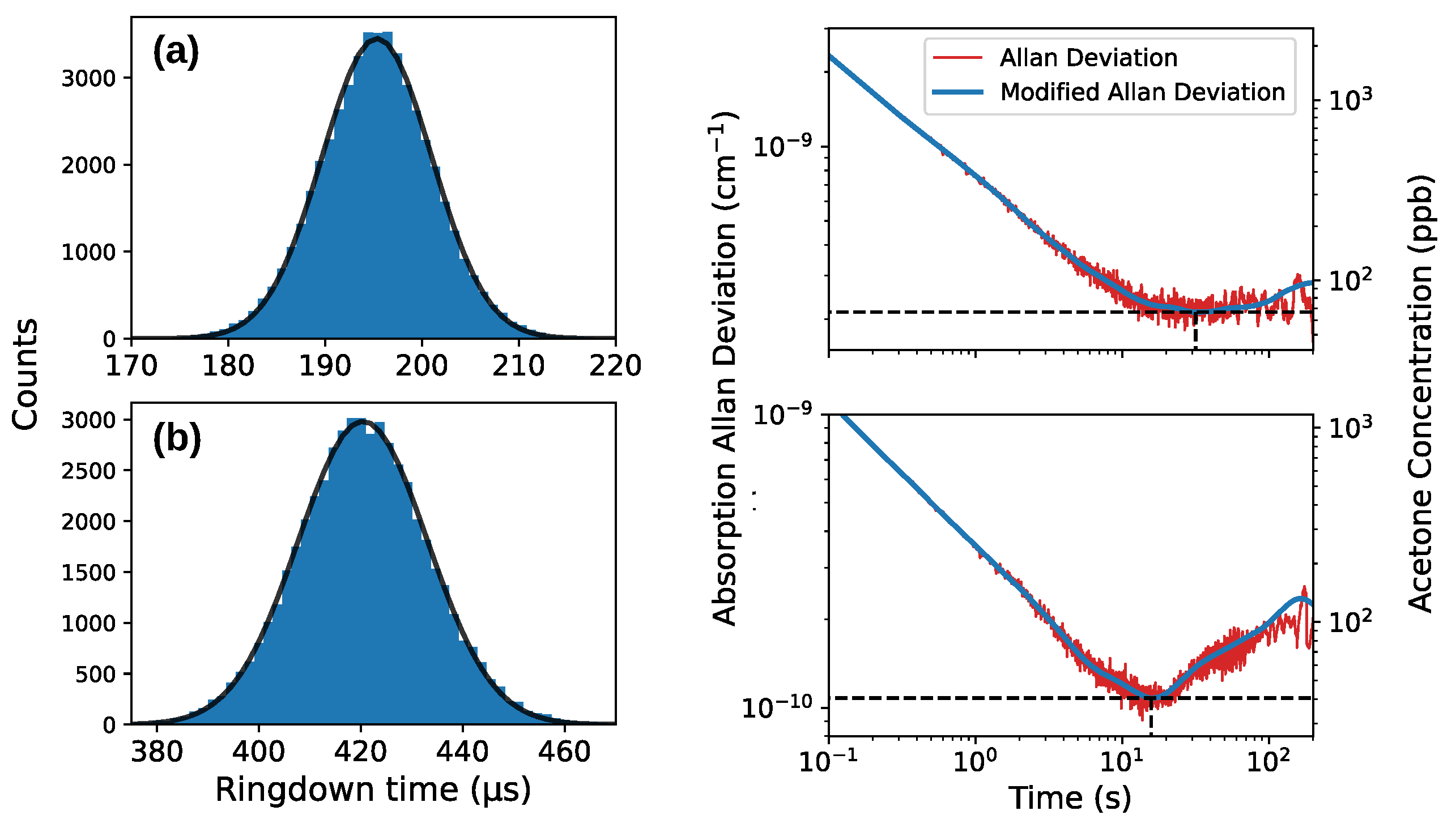
4.5. Detection Limit

We can evaluate the detection limit of our system by the fluctuations in the measured ring-down time [35] near the baseline. For a weak absorption, the measured ring-down time τ is nearly that of the empty cavity baseline τ 0 , and must be distinguished from the intrinsic fluctuations of the measurements. For a single ring-down measurement, the detection limit is defined as the absorption which produces a change in ring-down time equal to the standard deviation of the baseline ring-down time Δ τ . This gives the detection limit of a single ring-down measurement as
Δ α = 1 c τ 0 2 Δ τ
When the measurement is conducted, many averages of the ring-down time are taken at each wavelength to effectively reduce the deviation Δ τ of the measurements. However, this cannot be continued indefinitely due to drift. The modified Allan variance [35] can be used to determine the optimum averaging time and the minimum possible value of Δ τ that can be obtained through averaging. This allows the minimum detectable absorption to be determined. Equivalently, we can calculate the Allan variance directly from measurements of the absorption coefficient to give directly the minimum variance of absorption coefficient Δ α . This is shown in Figure 8, where the minimum of the modified Allan deviation of the absorption coefficient gives the (1 σ ) minimum detectable absorption. For 15.8 s of averaging time, we obtained a detection limit of 1.1 × 10 10 cm−1. This corresponds to an acetone concentration of 44 ppb at 70 Torr when the absolute value of the peak absorption cross-section is considered, and 134 ppb when just the height of the characteristic peak is considered.

5. Discussion

The overtone absorption bands, as the C-H stretch band that we investigate in this paper, appear due to anharmonicity [36]. The overtones with relatively high transition frequencies, observed in the NIR region, involve primarily small mass hydrogen atoms coupled with larger atoms [37].
The profiles of the overtone absorption bands often show similarity with the profiles of the corresponding bands of fundamental wavelength. Indeed, the fundamental band [38] around ν f = 3320 cm−1 and the overtone absorption band that we are investigating around ν 0 = 5979 cm−1 both show a central peak on an elevated base. The anharmonicity is reflected in the fact that ν 0 < 2 ν f and leads to the frequency of the overtone being smaller than the corresponding multiple of the fundamental frequency. This was used for the determination of the molecular structure from spectroscopy of overtones [39]. The assignment of the observed band to the first overtone 2 ν a of the asymmetric stretching vibration of the methyl group CH3 of acetone with certainty follows from previous research [33,40,41].
Our determination of the absorption cross-section is based on the formula of Equation (8) and is not relying on the known cross-section of acetone for a different absorption band (in UV) as in ref. [23]. Strictly speaking, Equation (13) determines the total attenuation cross-section, which also includes losses due to scattering. To the scattering losses contribute all gas components that are present in the optical cavity. However, the scattering cross-section at the used wavelengths is many orders of magnitude smaller than the absorption cross-section [42] and can be neglected. We note that the absorption from hot band transitions [43] at our temperature is also negligible.
We performed measurements with a mixture of gases and used the well-known absorption cross-sections of methane, water, and carbon dioxide in the NIR region. The relatively high concentration of acetone and methane compared to other VOCs and high spectral resolution made it possible to accurately determine their concentrations in gas mixtures of exhaled breath. The peak value of the acetone NIR cross-section and position of the peak absorption for the investigated absorption band are shown in Table 3 in comparison to the values obtained in previous research. The obtained value of the peak absorption of 1.22 × 10 21 cm 2 is in good agreement with refs. [33,40,44], and the position of the peak of 1672.4 nm is also in good agreement with refs. [25,40].
Some variations in the observed absorption and consequently in the retrieved acetone concentration as determined from spectroscopic measurements can be related to the equilibration process after the admission of the gaseous sample into the chamber, partial condensation, and interactions in the mixture of acetone and water molecules. Such mixtures can show azeotropic behavior [45], adsorption effects on condensed fraction and on the walls of the chamber [46,47], and interactions due to hydrogen bonds [48,49,50]. These effects can be especially important before the equilibrium is achieved. Indeed, in our measurements, the initially observed absorption gradually reduced by about 10% on a time scale of hours, as seen in Figure 6.
Our measurements with diluted samples of the calibration gas show that the achieved detection limit for acetone of 44 ppb at 70 Torr total pressure and 15.8 s integration time is low enough for the analysis of human breath samples, since the typical range of concentrations even for healthy individuals is from 0.2 ppm to 1.03 ppm [1]. This is comparable in sensitivity with the MIR sensor employing a 7.32 µm quantum cascade laser and a multi-pass cell [51], which demonstrated the detection limit of 21.4 ppb with a 78 s integration time. Note that our sensor does not require any preliminary acetone enrichment or separation as is the case for acetone detection with a chemoresistive sensor combined with a catalytic filter and separation column [52]. Despite a relatively narrow measured spectral interval (as compared, for instance, to the frequency comb spectroscopy [19]), it also enables the detection of methane as is shown in Figure 7 and Table 2, which often requires a specialized sensor [53]. The high spectral resolution allowed for the identification of spectral lines contributed by different isotopes, as presented in Table 2. Of particular interest are carbon isotopes for breath analysis [54] and for monitoring atmospheric environments [55].

6. Conclusions

We performed cavity ring-down spectroscopy of the C-H stretch overtone absorption band in the NIR spectral range of 1671.5–1675.0 nm. The absorption cross-section was determined from the measurements with calibration gas and its mixtures with breath samples. We have shown that a simple empirical model gives good agreement with the absorption cross-section of dilute acetone gas in the measured wavelength range. The peak absorption value of 1.22 × 10 21 cm 2 positioned at 1672.442 nm in the investigated spectral range is in agreement with some of the previous measurements. The absorption peak of acetone is distinct enough from those of other molecules present in human breath to allow for quantitative analysis of acetone in human breath samples. These measurements required multispecies analysis of gas mixtures that was developed and demonstrated on human breath samples. Some variations in the observed absorption of acetone due to interactions with water and the walls of the measuring chamber were observed and discussed. The detection limit down to 44 ppb at 70 Torr total pressure in the chamber with 15.8 s integration time was demonstrated as sufficient for sensitive analysis of exhaled breath. Thus, the measurements of the C-H stretch overtone absorption band within the tuning range of a diode laser present a viable and inexpensive approach to measure acetone content in exhaled breath.

Author Contributions

Conceptualization, J.B., H.S. and E.A.; methodology, J.B., H.S. and A.K.; software, J.B.; validation, A.K. and H.S.; formal analysis, J.B.; investigation, J.B. and E.A.; resources, A.K. and H.S.; data curation, J.B.; writing—original draft preparation, J.B. and A.K.; writing—review and editing, J.B. and A.K.; visualization, J.B.; supervision, H.S.; project administration, H.S.; funding acquisition, H.S. and A.K. All authors have read and agreed to the published version of the manuscript.

Funding

This research was supported in part by Robert Welch Foundation, grant A1546.

Data Availability Statement

The original contributions presented in the study are included in the article, further inquiries can be directed to the corresponding author.

Acknowledgments

The authors would like to thank Timothy Johnson of Pacific Northwest National Laboratory for providing quick and easy access to the broadband acetone spectrum, which significantly facilitated our investigation.

Conflicts of Interest

The authors declare no conflicts of interest.

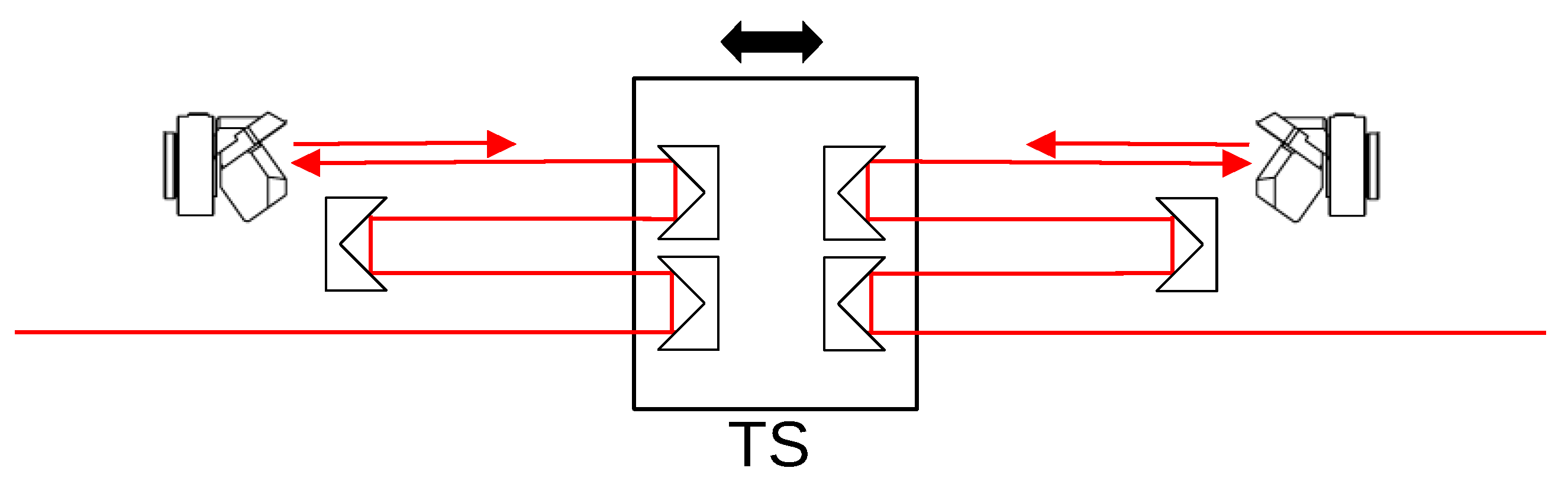
Appendix A. Wavelength Measurement

The DFB laser wavelength was measured at the zero-order output of the AOM using a scanning Michelson interferometer. This wavelength is measured relative to a reference laser, which in this case is a Zeeman stabilized helium neon laser, by counting the number of zero crossings which occur in the interference fringes of the two lasers. Using the arrangement shown in Figure A1, we measure these interference fringes separately for each laser and record the times of zero crossings. The wavelength of the DFB laser λ DFB can be estimated from
λ DFB N HeNe N DFB λ HeNe
where N HeNe / N DFB is the ratio of the number of zero crossings in the two interference fringes, and the known reference laser wavelength is λ HeNe . The counting error in the zero crossing number can be reduced [56] by recording the time information of the zero crossings, resulting in a much improved estimate of the wavelength than that given by Equation (A1), but still proportional to the known reference laser wavelength λ HeNe . This improved estimate was used in our measurements.
The wavelength is measured at ambient pressure, and there is an expected mismatch between the refractive index inside the chamber and the ambient air in which wavelength is measured. Additionally, the reference laser is stabilized against short-term drifts, but long-term drifts of the reference laser wavelength are possible. The combination of these two effects requires a correction to the measured wavelength λ meas by multiplying by a constant factor p λ
λ = p λ λ meas
In this investigation, the measured spectra all contained contributions from water vapor. As can be seen from Figure 3, these absorptions from water vapor are narrow and serve as well-defined markers of wavelength. The vacuum wavelengths of the water vapor lines are used to find the value of the correction factor p λ . We do this by scaling the wavelength axis of the measurements so that the observed absorption peaks attributed to water vapor occur at the vacuum wavelengths which are predicted by the parameters in the HITRAN database [30].

Interferometric Wavemeter

The design of the home-made wavemeter is shown in Figure A1 and the arrangement of the back reflectors allowing for a 16 times multiplication of the translation stage distance is presented in Figure A2.
The repeatability of the wavelength measurements using this instrument is better than one part in 10 8 when a full scan of the 5.2 m delay distance is performed. This is accomplished by folding the beam many times in the delay arms to extend the available scanning distance to 16 times that of the 325 mm translation stage (Newport DL325). This folding can be seen in Figure A2.
For the measurements conducted in this investigation, a scan step consists of a laser wavelength change of ∼0.03 nm. The full precision of the instrument was not necessary for resolving these scan steps, and we instead measured wavelength with a shorter delay, allowing for quicker measurements. A 0.4 m scan of delay was chosen and five separate measurements of wavelength were performed in a single movement of the translation stage lasting two seconds. The median of these values was assigned to be the wavelength of each spectrum point.
Figure A1. Simplified diagram of home-made wavemeter consisting of a symmetric Michelson interferometer aligned to a reference He-Ne laser and fiber collimator (FC). The central beam-splitter (BS) and compensation plate (CP) form two arms of variable distance which is scanned by a translation stage (TS). The retro-reflector configuration is such that the return beam from each arm is anti-parallel and displaced. Two pairs of spatially separated beams are obtained at the BS; one pair, consisting of two overlapped reference He-Ne beams (shown in red), is directed to a Si photodiode (PD). The other pair is formed by two IR beams (shown in blue) and is directed to the InGaAs detector. The IR input of the instrument is connected via a single mode fiber to ensure consistent beam profile and pointing direction.
Optics 06 00009 g0a1
Figure A2. Expanded view of translation stage and retro-reflectors. Multiple passes and translation of both interferometer arms allow for a total of 16 times multiplication of the translation stage distance.
Optics 06 00009 g0a2

Appendix B. Choice of Weighting Function

For this discussion, we will drop the dependence on the wavelength of the baseline ring-down time τ 0 ( λ ) τ 0 and assume it is constant. This is both for notational simplicity and because it is a valid approximation for our experimental conditions, as evidenced by Figure 7.
Throughout the investigation, we fit models which were linear combinations of known functions
α m ( λ ) = a 0 σ 0 ( λ ) + + a 1 σ n ( λ )
having unknown proportional coefficients. These proportional coefficients are determined by setting up the over-determined system
α 1 α 2 α 3 α N = σ 1 ( λ 1 ) σ 2 ( λ 1 ) σ m ( λ 1 ) σ 1 ( λ 2 ) σ 2 ( λ 2 ) σ m ( λ 2 ) σ 1 ( λ 3 ) σ 2 ( λ 3 ) σ m ( λ 3 ) σ 1 ( λ N ) σ 2 ( λ N ) σ m ( λ N ) a 1 a 2 a m
and then the least-squares solution to the above system is given at once by
a = ( A T A ) 1 A T α
where A is the N by m matrix in (A4), α is a vector containing the absorption measurements calculated from
c α i c α ( τ i ) = τ i 1 τ 0 1
The set of coefficients a j given by this solution are such that the quantity
E α = i α i α m ( λ i ) 2 = i 1 c 1 τ i 1 τ 0 α m ( λ i ) 2
is minimized. A potential problem with this scheme is that the deviation in the absorption measurements Δ α is not homoscedastic and the deviation changes over the potential range of absorption magnitudes.
For a ring-down time measurement dominated by technical noise rather than systematic effects, the relative deviation of these measurements Δ τ / τ ¯ is approximately constant [57], where τ ¯ is the mean of the measurements. This behavior is confirmed in our experiment, as indicated by the histograms in Figure 8. If we transform the measurements by a function f ( τ ) , then the deviations in the resulting function values are Δ f = f ( τ ¯ ) Δ τ . Choosing f ( τ ) = ln ( τ / τ 0 ) gives a variance Δ f = Δ τ / τ ¯ which is approximately constant. This implies that we should minimize the error in log-space
E L = i ln τ i τ 0 ln τ model ( λ i ) τ 0 2 = i ln τ i τ 0 + ln 1 + c τ 0 α m ( λ i ) 2
where we have the simulated ring-down time from the inverse of Equation (A6) applied to the model absorption
τ model ( λ ) = 1 c α m ( λ ) + 1 / τ 0
We will also consider the solution which minimizes the error sum in the space of ring-down time
E τ = i τ i 1 c α m ( λ i ) + 1 / τ 0 2
Unlike E α , the unknown a i coefficients do not appear linearly in the transformed errors E L and E τ , and the solutions for a i which minimize these sums cannot be written as a simple equation. We instead proceed by choosing a weight function which transforms the solution for E α into one which approximates that of E L or E τ .
The set of N equations given by (A4) can each be multiplied by a constant factor without affecting the equality of each equation. If we choose this factor to depend on the value of the ring-down time measurement w ( τ i ) , then the least-squares solution (A5) is affected by shifting the relative importance of each equation in the sum. The least-squares solution which is obtained from the weighted set of equations is that which minimizes the sum
E α , w = i α ( τ i ) w ( τ i ) α m ( λ i ) w ( τ i ) 2
We analyze this sum by Taylor expanding the terms separately for small absorption. Specifically, we expand the left term about the corresponding point of ring-down time nearly equal to the baseline τ τ 0 , and the right term about the point of zero absorption c τ 0 α m 0 .
E α , w 1 c τ 0 2 i [ A 1 τ i τ 0 τ 0 + A 2 τ i τ 0 τ 0 2 + + w ( τ 0 ) c τ 0 α m ( λ i ) + c τ 0 α m ( λ i ) w ( τ i ) w ( τ 0 ) ] 2
where the
A n = ( 1 ) n 1 k = 0 n 1 ( τ 0 ) k k ! w ( k ) ( τ 0 )
result from the Taylor expansion of α ( τ i ) w ( τ i ) about the point τ 0 , and the use of the generalized Leibniz rule to evaluate the derivative terms. We give the first few values of the number A n which are expressed as derivatives of the weight function evaluated at the baseline ring-down time
A 1 = w ( τ 0 )
A 2 = τ 0 w ( τ 0 ) w ( τ 0 )
A 3 = 1 2 τ 0 2 w ( τ 0 ) τ 0 w ( τ 0 ) + w ( τ 0 )
It can be seen that the A n obey the recursion relation
A n + 1 = ( τ 0 ) n n ! w ( n ) ( τ 0 ) A n
We expand the expression (A10) for E τ in small absorption
E τ τ 0 2 i τ i τ 0 τ 0 + c τ 0 α m c 2 τ 0 2 α m 2 +
First-order agreement between the expansions of E α , w and E τ in (A12) and (A18) for small ( τ i τ 0 ) / τ 0 and c τ 0 α m is obtained when we set w ( τ 0 ) = 1 . We can achieve something like second-order agreement if we assign A 2 = 0 and w ( τ i ) w ( τ 0 ) = c τ 0 α ( τ i ) . Since we do have a priori knowledge of the model prediction at the measurement wavelength α m ( λ i ) , we instead use the measured absorption coefficient α i to make the expansion agree to second order. Using (A6), we make the replacement c τ 0 α m ( λ i ) τ 0 τ i 1 τ i τ 0 τ 0 and we then have
w ( τ i ) w ( τ 0 ) ( τ i τ 0 ) / τ 0
The assignment A 2 = 0 gives for the first derivative of the weight function w ( τ 0 ) = 1 / τ 0 . This condition combined with w ( τ 0 ) = 1 gives the first-order Taylor expansion of the weight function as
w τ ( τ ) = 1 + τ τ 0 τ 0 = τ τ 0
It can be seen that this expression agrees with the condition (A19). If we try to continue the process to higher order, then we must demand that A 3 = 0 , which immediately gives w ( τ 0 ) = 0 , and a truncation of the Taylor series. It was confirmed in the simulations of Appendix C that the weight function w τ ( τ ) consistently yielded the smallest values for E τ compared to the other weight functions considered in this work.
We can perform a similar analysis on the expansion of the log-space error E L given by (A8) in small absorption
E L i [ τ i τ 0 τ 0 τ i τ 0 2 2 τ 0 2 + τ i τ 0 3 3 τ 0 4 + c τ 0 α m ( λ i ) + c τ 0 α m ( λ i ) 1 2 c τ 0 α m ( λ i ) + 1 3 c 2 τ 0 2 α m 2 ( λ i ) ] 2
First-order agreement between (A12) and (A21) is again obtained when we set w ( τ 0 ) = 1 . Second-order agreement of the two expansions in ( τ i τ 0 ) / τ 0 is obtained when we set A 2 = 1 / 2 which gives w ( τ 0 ) = 1 / 2 τ 0 .
To compare the terms in the parentheses of (A21) to equivalent terms in the weighted sum (A12), we must linearize these terms in the absorption model α m . We replace the higher-order terms of α m with the measured absorption α i using the rule c τ 0 α m ( λ i ) τ 0 τ i 1 . This gives the auxiliary condition for agreement between (A12) and (A21)
w ( τ i ) w ( τ 0 ) 1 2 τ 0 τ i 1 τ i τ 0 2 τ 0
The condition above, along with w ( τ 0 ) = 1 and w ( τ 0 ) = 1 / 2 τ 0 , is satisfied by w L ( τ ) 1 + τ τ 0 2 τ 0 . Note that this linear function is already determined by the conditions on w ( τ 0 ) and w ( τ 0 ) , but happens to also fulfill the auxiliary condition.
We can continue this process to higher order indefinitely by setting A n = ( 1 ) n + 1 / n to match each term appearing from the expansion of ln τ i / τ 0 . From (A17), we can then solve for the nth derivative of the weight function
w ( n ) ( τ 0 ) = n ! ( 1 ) n 1 τ 0 n 1 n 1 n + 1
allowing us to construct the full Taylor series for the weight function
w L ( τ ) = 1 + n = 1 ( 1 ) n 1 1 n 1 n + 1 τ τ 0 τ 0 n
This sum can be seen to equal
w L ( τ ) = τ ln τ τ 0 τ τ 0
The weight function w L ( τ ) we have constructed also satisfies the same auxiliary condition demanded earlier to all orders
w L ( τ i ) w L ( τ 0 ) = 1 2 τ 0 τ i 1 + 1 3 τ 0 τ i 1 2 1 4 τ 0 τ i 1 3 +
which is obtained using the replacement c τ 0 α m ( λ i ) τ 0 τ i 1 in the parenthetical terms of Equation (A21) and comparing to (A12).
The expansion of ln ( 1 + c τ 0 α m ) used to go from (A8) to (A21) is only valid for c τ 0 α m 1 . This can be improved if instead we expand about the point c τ 0 α m = 1 , giving an improved radius of convergence up to a larger absorption of c τ 0 α m 3 . We must correspondingly expand ln ( τ / τ 0 ) about the point τ = τ 0 / 2 . The radius of convergence of this expansion still captures the entire dynamic range 0 < τ < τ 0 . The result of performing the above process about this new expansion point and normalizing to w ( τ 0 ) = 1 is the weighting function
w L 2 ( τ ) = w L ( 2 τ ) / w L ( 2 τ 0 )
It was found in the simulations of Appendix C that the weight functions (A25) and (A27) both lower the value of the error E L compared to the unweighted least squares solution, indicating that our process was successful. Additionally, it was found that the use of these weighting functions improved the accuracy of gas concentration determination in simulated datasets, especially as noise becomes large. The effect is largest for gas species having absorption features which encompass a significant fraction of the measurement dynamic range, where the absorption feature results in ring-down measurements spanning a range of at least τ 0 / 3 .
We show explicitly here the process of solving the weighted system. We can construct the system as we did earlier in (A4) but we modify the system by multiplying each term by w ( τ i ) giving the weighted system
α 1 w ( τ 1 ) α 2 w ( τ 2 ) α 3 w ( τ 3 ) α N w ( τ N ) = σ 1 ( λ 1 ) w ( τ 1 ) σ 2 ( λ 1 ) w ( τ 1 ) σ m ( λ 1 ) w ( τ 1 ) σ 1 ( λ 2 ) w ( τ 2 ) σ 2 ( λ 2 ) w ( τ 2 ) σ m ( λ 2 ) w ( τ 2 ) σ 1 ( λ 3 ) w ( τ 3 ) σ 2 ( λ 3 ) w ( τ 3 ) σ m ( λ 3 ) w ( τ 3 ) σ 1 ( λ N ) w ( τ N ) σ 2 ( λ N ) w ( τ N ) σ m ( λ N ) w ( τ N ) a 1 a 2 a m
The weighted least squares solution is given at once by
a = ( A T A ) 1 A T α
where the A and α are the above N by m matrix and length-N vector, respectively, which have their terms multiplied by the weight function w ( τ ) .

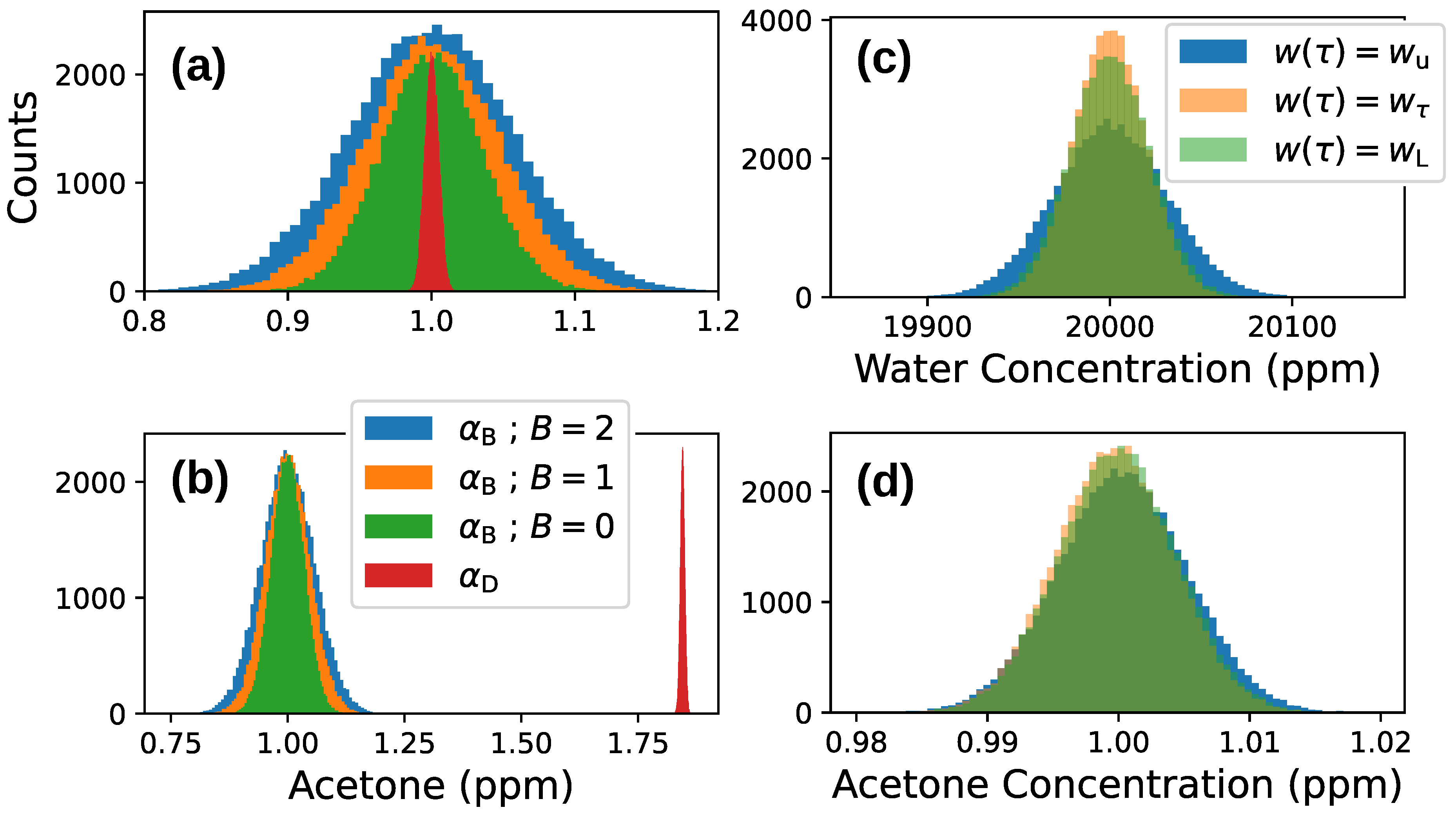
Appendix C. Simulation of Fitting Procedure

We perform Monte Carlo simulation of the effect of ring-down time measurement noise on the fitting process and compare the effect of using different weighting functions on simulated breath samples. From the simulations, we are able to estimate uncertainty in the concentrations of all gas species measured in this investigation as well as quantify the effect of using different weighting functions and artificial baselines.
We simulated a breath spectrum similar to Figure 7 containing 1 ppm acetone at 70 Torr. Using parameters in the HITRAN database [30] and the concentrations y i shown in the right-most column of Table A1, we simulated the absorption cross6section of all components reported in Figure 7 and summed them to give a simulated breath spectrum α ( λ ) = P k B T i y i σ i ( λ ) . We added to this spectrum the expected absorption of 1 ppm acetone using the model reported in this paper.
We converted the simulated breath spectrum into a curve of τ ( λ ) using a typical fit of the baseline ring-down time τ 0 ( λ ) and added Gaussian noise. At each simulated wavelength λ i , the deviation Δ τ of this Gaussian noise was chosen to be proportional to τ ( λ i ) , which is typical of ring-down measurements limited by statistical noise [57]. To model the performance of our spectrometer, the value of Δ τ / τ was chosen to be 0.003, which is typical of a measurement of our setup having 100 averages. This number of averages is well within the linear portion of the dependence shown in the right of Figure 8 and corresponds to a Δ τ , which is decreasing as the square root of the number of averages.
For each of these simulated noisy ring-down measurements τ i , we converted them to absorption using α i = ( τ i 1 τ 0 1 ( λ i ) ) / c and with Equation (A29) found the set of concentrations y i which give the weighted least squares fit (A29) of the simulated breath spectrum. We evaluated the four weighting functions
w u ( τ ) = 1 w τ ( τ ) = τ τ 0 w L ( τ ) = τ ln τ τ 0 τ τ 0 w 2 L ( τ ) = w L ( 2 τ ) w L ( 2 τ 0 )
on the performance of the recovered concentrations as well as monitored the root mean square deviations E α , E τ , E L , and E 2 L .
We additionally tested the performance of different models of the absorption baseline. For the fitting model, we used the model absorption directly with the offset term
α D ( λ ) = a 0 σ ac ( λ ) + i a i σ i ( λ ; T , P )
and compared this to the modified absorption model
α B ( λ ) = a 0 σ ˜ ac ( λ ) + n = 0 B b n ( λ λ 0 ) n + i a i σ i ( λ ; T , P )
where σ ˜ ac is normalized peak function from Equation (10). This modification allows us to determine the acetone cross-section independently of baseline errors, essentially only using the shape of the broadband peak for concentration determination. The sum over n is a function used to model the baseline and is a polynomial of order B. The term λ 0 is a term used to center the terms in the range of the scan and we used a value of λ 0 = 1673.5 nm for both simulation and data analysis in this work. The sum over i is over the different molecular cross-sections modeled using the HITRAN database at a temperature of T = 296 K and P = 70 Torr.
The coefficients a 0 , i give the gas component concentrations from (14) and the b n coefficients define the polynomial baseline. Both sets of coefficients are determined using (A29) and we compare the different weighting functions w u ( τ ) , w τ ( τ ) , and w L ( τ ) . The choice of λ 0 affects the b i coefficients, but gives the same resulting polynomial when expanded for a particular simulated spectrum. However, the numerical stability of the routine used to evaluate (A29) can be improved by choosing λ 0 in the center of the scan and normalizing the small cross-section values for each species.
The results are shown in Figure A3 and Table A1 and Table A2. The use of different baseline polynomial orders B did not significantly affect the determination of the concentrations of the different gas species calculated from the HITRAN database since these correspond to narrow spectrum features. However, since acetone concentration is determined from a broadband feature, the accuracy of concentration determination was generally degraded with increasing B.
The model α D ( λ ) gave the best results when the offset of the absorption feature could be definitively determined, as seen in Figure A3a. The results of adding a constant offset of 2 × 10 9 cm−1 to the simulated absorption spectra can be seen in Figure A3b, where the α D ( λ ) model is severely displaced from the expected mean of 1 ppm acetone concentration. The α B ( λ ) models showed complete immunity to this shift at the expense of higher deviations in the concentration estimate. Although the increased deviations of the α B ( λ ) models became worse as the baseline polynomial order B increased, they were increasingly immune to distortions of the baseline.
Shown in Table A1 and Table A2 are the relative errors in the concentrations of various gas species resulting from the fitting process for simulated experimental conditions. The values shown in the table are in agreement with the experimental data repeatability. The choice of weighting function used to fit the simulated spectra did not significantly affect the results for simulated experimental conditions, except for the most common isotopologue of water (see Figure A3c) and acetone (see Figure A3d). Since the absorption peaks of water encompass the largest dynamic range of the measurement, the effect of the weighting function is largest on this species.
To further investigate the effect of the weighting functions on the recovered concentrations, we additionally simulated 100,000 spectra which had a much larger relative noise of Δ τ / τ = 5 % . Under the condition of increased noise, the choice of weighting function had a larger effect which can be seen in the results of Table A3. The unweighted fitting procedure tended to slightly overestimate the gas concentrations, while the weighting function w τ tended to slightly underestimate concentrations. The weighting functions w L and w L 2 gave the best agreement to the exact values and produced the only results which agreed to the exact values’ one standard error.
We conclude from these simulations that the best performance is offered by the weighting functions w L and w L 2 given by Equations (A25) and (A27). The direct fitting model α D given by Equation (A30) gave the best performance in terms of acetone concentration estimation. However, in the case where the absorption baseline cannot be determined or has some distortion, the best results are then offered by the α B ( λ ) model given by Equation (A31) with B chosen to capture the effect of the distortion.
Figure A3. Simulation results showing histograms of recovered concentrations from a simulated breath spectrum spectrum having 1000 points evenly spaced in the range of 1671.5–1675 nm superimposed with Gaussian noise characterized by Δ τ / τ = 0.3 % . Shown in (a,b) is the effect of changing the absorption model. It can be seen in (a) that the best acetone concentration estimate is obtained using the direct model α D ( λ ) , but suffers from sensitivity to baseline offset. Seen in (b) are the results where a constant 2 × 10 9 cm−1 absorption was added to the simulated spectra, causing a severe shift of the mean acetone concentration recovered by the α D model. Shown in (c,d) is the effect of the weighting function w ( τ ) . The improvement to the water concentration estimate when using the weighting function is shown in (c). A slightly improved acetone concentration estimate is also obtained when using the weight function, as seen in (d).
Optics 06 00009 g0a3
Table A1. Relative error calculated for each gas concentration y i as the ratio of the standard deviation to the mean for a set of simulated breath sample measurements having noise characterized by Δ τ / τ = 0.3 % . These results are essentially the same for the different weighting functions with the exception of H2O and acetone (marked with * in the table), which are shown with the values obtained using the specf w ( τ ) = τ / τ 0 . The results are also nearly identical for the different models with the exception of acetone, which is shown with the results from the direct fitting model α D .
SpeciesRelative ErrorConcentration
(ppm)
CH40.26%2
13CH421%0.02246
H2O *0.10%23,000
CO20.33%32,000
13CO21.2%359.36
CO(18O)0.32%128.32
CO(17O)7.9%24.0
H2(18O)9.6%46.0
Acetone *0.45%1.0
Table A2. The effect of the diffent models α D and α B for different values of B on the concentration of acetone extracted from the fits of a set of 50,000 simulated breath sample measurements having noise characterized by Δ τ / τ = 0.3 % . The relative error is calculated as the standard deviation divided by the mean, and can be seen graphically in Figure A3a. These simulations reflect the situation where there is no unknown offset or distortion in the absorption baseline.
ModelAcetone Relative Error
α D 0.45%
α B = 0 3.3%
α B = 1 4.6%
α B = 2 5.5%
Table A3. Results of using the different weight functions discussed in this work to fit 100,000 simulated measurements of a breath sample having a particularly large relative noise of Δ τ / τ = 5 % . Shown is the average of the concentration estimates in parts-per-million for some select gas species. The percentage shown is the relative error, computed as the ratio of the standard deviation of these estimates to their mean. The weight functions w L and w L 2 are seen to give the most accurate estimate of the gas concentrations. On average, the unweighted estimates are seen to slightly overestimate the concentrations, and the weight function w τ is seen to slightly underestimate concentrations.
Weight FunctionCH4H2OCO2 CO(18O)Acetone
w ( τ ) = 1 2.00620,051.732,080.3128.71.0860
(Unweighted)4.5%2.6%5.5%5.4%7.6%
w ( τ ) = w τ 1.99919,953.131,955.6128.00.9125
4.4%1.7%5.4%5.3%8.3%
w ( τ ) = w L 2.00219,991.232,005.1128.30.9987
4.4%1.8%5.4%5.3%7.6%
w ( τ ) = w L 2 2.00219,996.532,012.5128.41.0087
4.5%1.9%5.4%5.3%7.5%
Exact2.020,000.032,000.0128.321.0

References

  1. Wang, Z.; Wang, C. Is breath acetone a biomarker of diabetes? A historical review on breath acetone measurements. J. Breath Res. 2013, 7, 037109. [Google Scholar] [CrossRef]
  2. Marcondes-Braga, F.G.; Gioli-Pereira, L.; Bernardez-Pereira, S.; Batista, G.L.; Mangini, S.; Issa, V.S.; Fernandes, F.; Bocchi, E.A.; Ayub-Ferreira, S.M.; Mansur, A.J.; et al. Exhaled breath acetone for predicting cardiac and overall mortality in chronic heart failure patients. ESC Heart Fail. 2020, 7, 1744–1752. [Google Scholar] [CrossRef]
  3. Marcondes-Braga, F.G.; Gutz, I.G.R.; Batista, G.L.; Saldiva, P.H.N.; Ayub-Ferreira, S.M.; Issa, V.S.; Mangini, S.; Bocchi, E.A.; Bacal, F. Exhaled acetone as a new biomaker of heart failure severity. Chest 2012, 142, 457–466. [Google Scholar] [CrossRef]
  4. Owen, O.E.; Trapp, V.E.; Skutches, C.L.; Mozzoli, M.A.; Hoeldtke, R.D.; Boden, G.; Reichard, G.A., Jr. Acetone Metabolism During Diabetic Ketoacidosis. Diabetes 1982, 31, 242–248. [Google Scholar] [CrossRef]
  5. Stafstrom, C.E.; Rho, J.M. Epilepsy and the Ketogenic Diet; Springer Science and Business Media: New York, NY, USA, 2004. [Google Scholar]
  6. Singh, H.B.; O’Hara, D.; Herlth, D.; Sachse, W.; Blake, D.R.; Bradshaw, J.D.; Kanakidou, M.; Crutzen, P.J. Acetone in the atmosphere: Distribution, sources, and sinks. J. Geophys. Res. Atmos. 1994, 99, 1805–1819. [Google Scholar] [CrossRef]
  7. Schade, G.W.; Goldstein, A.H. Seasonal measurements of acetone and methanol: Abundances and implications for atmospheric budgets. Glob. Biogeochem. Cycles 2006, 20, GB1011. [Google Scholar] [CrossRef]
  8. Snyder, L.E.; Lovas, F.J.; Mehringer, D.M.; Miao, N.Y.; Kuan, Y.J.; Hollis, J.M.; Jewell, P.R. Confirmation of Interstellar Acetone. Astrophys. J. 2002, 578, 245. [Google Scholar] [CrossRef]
  9. Lykke, J.M.; Coutens, A.; Jørgensen, J.K.; van der Wiel, M.H.D.; Garrod, R.T.; Müller, H.S.P.; Bjerkeli, P.; Bourke, T.L.; Calcutt, H.; Drozdovskaya, M.N.; et al. The ALMA-PILS survey: First detections of ethylene oxide, acetone and propanal toward the low-mass protostar IRAS 16293-2422. Astron. Astrophys. 2017, 597, A53. [Google Scholar] [CrossRef]
  10. Kosterev, A.A.; Malinovsky, A.L.; Tittel, F.K.; Gmachl, C.; Capasso, F.; Sivco, D.L.; Baillargeon, J.N.; Hutchinson, A.L.; Cho, A.Y. Cavity ringdown spectroscopic detection of nitric oxide with a continuous-wave quantum-cascade laser. Appl. Opt. 2001, 40, 5522–5529. [Google Scholar] [CrossRef]
  11. Manne, J.; Sukhorukov, O.; Jäger, W.; Tulip, J. Pulsed quantum cascade laser-based cavity ring-down spectroscopy for ammonia detection in breath. Appl. Opt. 2006, 45, 9230–9237. [Google Scholar] [CrossRef]
  12. Wang, C.; Surampudi, A.B. An acetone breath analyzer using cavity ringdown spectroscopy: An initial test with human subjects under various situations. Meas. Sci. Technol. 2008, 19, 105604. [Google Scholar] [CrossRef]
  13. Ghorbani, R.; Schmidt, F.M. ICL-based TDLAS sensor for real-time breath gas analysis of carbon monoxide isotopes. Opt. Express 2017, 25, 12743–12752. [Google Scholar] [CrossRef]
  14. Philippe, L.C.; Hanson, R.K. Laser diode wavelength-modulation spectroscopy for simultaneous measurement of temperature, pressure, and velocity in shock-heated oxygen flows. Appl. Opt. 1993, 32, 6090–6103. [Google Scholar] [CrossRef]
  15. Xia, J.; Zhu, F.; Kolomenskii, A.A.; Bounds, J.; Zhang, S.; Amani, M.; Fernyhough, L.J.; Schuessler, H.A. Sensitive acetone detection with a mid-IR interband cascade laser and wavelength modulation spectroscopy. OSA Contin. 2019, 2, 640–654. [Google Scholar] [CrossRef]
  16. Thorpe, M.J.; Balslev-Clausen, D.; Kirchner, M.S.; Ye, J. Cavity-enhanced optical frequency comb spectroscopy: Application to human breath analysis. Opt. Express 2008, 16, 2387–2397. [Google Scholar] [CrossRef]
  17. Wang, C.; Sahay, P. Breath Analysis Using Laser Spectroscopic Techniques: Breath Biomarkers, Spectral Fingerprints, and Detection Limits. Sensors 2009, 9, 8230–8262. [Google Scholar] [CrossRef]
  18. Stacewicz, T.; Bielecki, Z.; Wojtas, J.; Magryta, P.; Mikolajczyk, J.; Szabra, D. Detection of disease markers in human breath with laser absorption spectroscopy. Opto-Electron. Rev. 2016, 24, 82–94. [Google Scholar] [CrossRef]
  19. Xia, J.; Zhu, F.; Bounds, J.; Aluauee, E.; Kolomenskii, A.; Dong, Q.; He, J.; Meadows, C.; Zhang, S.; Schuessler, H. Spectroscopic trace gas detection in air-based gas mixtures: Some methods and applications for breath analysis and environmental monitoring. J. Appl. Phys. 2022, 131, 220901. [Google Scholar] [CrossRef]
  20. Pangerl, J.; Moser, E.; Müller, M.; Weigl, S.; Jobst, S.; Rück, T.; Bierl, R.; Matysik, F.M. A sub-ppbv-level Acetone and Ethanol Quantum Cascade Laser Based Photoacoustic Sensor—Characterization and Multi-Component Spectra Recording in Synthetic Breath. Photoacoustics 2023, 30, 100473. [Google Scholar] [CrossRef]
  21. Szabó, A.; Ruzsanyi, V.; Unterkofler, K.; Mohácsi, A.; Tuboly, E.; Boros, M.; Szabó, G.; Hinterhuber, H.; Amann, A. Exhaled methane concentration profiles during exercise on an ergometer. J. Breath Res. 2015, 9, 016009. [Google Scholar] [CrossRef]
  22. Wang, C.; Mbi, A. A new acetone detection device using cavity ringdown spectroscopy at 266 nm: Evaluation of the instrument performance using acetone sample solutions. Meas. Sci. Technol. 2007, 18, 2731. [Google Scholar] [CrossRef]
  23. Cias, P.; Wang, C.; Dibble, T.S. Absorption Cross-Sections of the C—H Overtone of Volatile Organic Compounds: 2 Methyl-1,3-Butadiene (Isoprene), 1,3-Butadiene, and 2,3-Dimethyl-1,3-Butadiene. Appl. Spectrosc. 2007, 61, 230–236. [Google Scholar] [CrossRef] [PubMed]
  24. Harrison, J.J.; Humpage, N.; Allen, N.D.; Waterfall, A.M.; Bernath, P.F.; Remedios, J.J. Mid-infrared absorption cross sections for acetone (propanone). J. Quant. Spectrosc. Radiat. Transf. 2011, 112, 457–464. [Google Scholar] [CrossRef]
  25. Sharpe, S.W.; Johnson, T.J.; Sams, R.L.; Chu, P.M.; Rhoderick, G.C.; Johnson, P.A. Gas-Phase Databases for Quantitative Infrared Spectroscopy. Appl. Spectrosc. 2004, 58, 1452–1461. [Google Scholar] [CrossRef] [PubMed]
  26. Johnson, T.J.; Hughey, K.D.; Blake, T.A.; Sharpe, S.W.; Myers, T.L.; Sams, R.L. Confirmation of PNNL Quantitative Infrared Cross-Sections for Isobutane. J. Phys. Chem. A 2021, 125, 3793–3801. [Google Scholar] [CrossRef] [PubMed]
  27. Romanini, D.; Kachanov, A.; Sadeghi, N.; Stoeckel, F. CW cavity ring down spectroscopy. Chem. Phys. Lett. 1997, 264, 316–322. [Google Scholar] [CrossRef]
  28. Zalicki, P.; Zare, R.N. Cavity ring-down spectroscopy for quantitative absorption measurements. J. Chem. Phys. 1995, 102, 2708–2717. [Google Scholar] [CrossRef]
  29. Karman, T.; Gordon, I.E.; van der Avoird, A.; Baranov, Y.I.; Boulet, C.; Drouin, B.J.; Groenenboom, G.C.; Gustafsson, M.; Hartmann, J.M.; Kurucz, R.L.; et al. Update of the HITRAN collision-induced absorption section. Icarus 2019, 328, 160–175. [Google Scholar] [CrossRef]
  30. Gordon, I.E.; Rothman, L.S.; Hargreaves, E.R.; Hashemi, R.; Karlovets, E.V.; Skinner, F.M.; Conway, E.K.; Hill, C.; Kochanov, R.V.; Tan, Y.; et al. The HITRAN2020 molecular spectroscopic database. J. Quant. Spectrosc. Radiat. Transf. 2022, 277, 107949. [Google Scholar] [CrossRef]
  31. Laane, J. Chapter Optimal Signal Processing in Cavity Ring-Down Spectroscopy. In Frontiers of Molecular Spectroscopy, 1st ed.; Laane, J., Ed.; Elsevier: Amsterdam, The Netherlands, 2009. [Google Scholar]
  32. Istratov, A.A.; Vyvenko, O.F. Exponential analysis in physical phenomena. Rev. Sci. Instruments 1999, 70, 1233–1257. [Google Scholar] [CrossRef]
  33. Wang, C.; Scherrer, S.T.; Hossain, D. Measurements of Cavity Ringdown Spectroscopy of Acetone in the Ultraviolet and Near-Infrared Spectral Regions: Potential for Development of a Breath Analyzer. Appl. Spectrosc. 2004, 58, 784–791. [Google Scholar] [CrossRef] [PubMed]
  34. Kochanov, R.; Gordon, I.; Rothman, L.; Wcisło, P.; Hill, C.; Wilzewski, J. HITRAN Application Programming Interface (HAPI): A comprehensive approach to working with spectroscopic data. J. Quant. Spectrosc. Radiat. Transf. 2016, 177, 15–30. [Google Scholar] [CrossRef]
  35. Huang, H.; Lehmann, K.K. Long-term stability in continuous wave cavity ringdown spectroscopy experiments. Appl. Opt. 2010, 49, 1378–1387. [Google Scholar] [CrossRef] [PubMed]
  36. Sandorfy, C. Overtones and Combination Tones: Application to the Study of Molecular Associations. In Infrared and Raman Spectroscopy of Biological Molecules; Theophanides, T.M., Ed.; Springer: Dordrecht, The Netherlands, 1979; pp. 305–318. [Google Scholar]
  37. Weyer, L.; Lo, S.C. Spectra–Structure Correlations in the Near-Infrared. In Handbook of Vibrational Spectroscopy; John Wiley & Sons, Ltd.: Hoboken, NJ, USA, 2006. [Google Scholar] [CrossRef]
  38. Harrison, J.J.; Allen, N.D.; Bernath, P.F. Infrared absorption cross sections for acetone (propanone) in the 3µm region. J. Quant. Spectrosc. Radiat. Transf. 2011, 112, 53–58. [Google Scholar] [CrossRef]
  39. Henry, B.R. The local mode model and overtone spectra: A probe of molecular structure and conformation. Accounts Chem. Res. 1987, 20, 429–435. [Google Scholar] [CrossRef]
  40. Peale, R.E.; Muravjov, A.V.; Fredricksen, C.J.; Boreman, G.D.; Saxena, H.; Braunstein, G.; Vaks, V.L.; Maslovsky, A.V.; Nikifirov, S.D. Spectral signatures of acetone vapor from ultraviolet to millimeter wavelengths. Int. J. High Speed Electron. Syst. 2008, 18, 627–637. [Google Scholar] [CrossRef]
  41. Hanazaki, I.; Baba, M.; Nagashima, U. Orientational site splitting of methyl C-H overtones in acetone and acetaldehyde. J. Phys. Chem. 1985, 89, 5637–5645. [Google Scholar] [CrossRef]
  42. Penndorf, R. Tables of the Refractive Index for Standard Air and the Rayleigh Scattering Coefficient for the Spectral Region between 0.2 and 20.0 μ and Their Application to Atmospheric Optics. J. Opt. Soc. Am. 1957, 47, 176–182. [Google Scholar] [CrossRef]
  43. Levine, I. Quantum Chemistry; Pearson Advanced Chemistry Series; Pearson: London, UK, 2014; p. 73. [Google Scholar]
  44. Denzer, W.; Hancock, G.; Islam, M.; Langley, C.E.; Peverall, R.; Ritchie, G.A.D.; Taylor, D. Trace species detection in the near infrared using Fourier transform broadband cavity enhanced absorption spectroscopy: Initial studies on potential breath analytes. Analyst 2011, 136, 801–806. [Google Scholar] [CrossRef]
  45. Mahdi, T.; Ahmad, A.; Nasef, M.M.; Ripin, A. State-of-the-Art Technologies for Separation of Azeotropic Mixtures. Sep. Purif. Rev. 2015, 44, 308–330. [Google Scholar] [CrossRef]
  46. Duan, S.X.; Jayne, J.T.; Davidovits, P.; Worsnop, D.R.; Zahniser, M.S.; Kolb, C.E. Uptake of gas-phase acetone by water surfaces. J. Phys. Chem. 1993, 97, 2284–2288. [Google Scholar] [CrossRef]
  47. Chen, J.; Hsiung, G.; Hsu, Y.; Chang, S.; Chen, C.; Lee, W.; Ku, J.; Chan, C.; Joung, L.; Chou, W. Water adsorption–desorption on aluminum surface. Appl. Surf. Sci. 2001, 169–170, 679–684. [Google Scholar] [CrossRef]
  48. Coutinho, K.; Saavedra, N.; Canuto, S. Theoretical analysis of the hydrogen bond interaction between acetone and water. J. Mol. Struct. 1999, 466, 69–75. [Google Scholar] [CrossRef]
  49. Max, J.J.; Chapados, C. Infrared spectroscopy of acetone–water liquid mixtures. I. Factor analysis. J. Chem. Phys. 2003, 119, 5632–5643. [Google Scholar] [CrossRef]
  50. Max, J.J.; Chapados, C. Infrared spectroscopy of acetone–water liquid mixtures. II. Molecular model. J. Chem. Phys. 2004, 120, 6625–6641. [Google Scholar] [CrossRef]
  51. Li, G.; Liu, Y.; Jiao, Y.; Zhang, Z.; Wu, Y.; Zhang, X.; Zhao, H.; Li, J.; Song, Y.; Li, Q.; et al. Mid-infrared acetone sensor for exhaled gas using FWA-LSSVM and empirical mode decomposition algorithm. Measurement 2023, 213, 112716. [Google Scholar] [CrossRef]
  52. Bastide, G.M.G.B.H.; Remund, A.L.; Oosthuizen, D.N.; Derron, N.; Gerber, P.A.; Weber, I.C. Handheld device quantifies breath acetone for real-life metabolic health monitoring. Sens. Diagn. 2023, 2, 918–928. [Google Scholar] [CrossRef]
  53. Kwaśny, M.; Bombalska, A. Optical Methods of Methane Detection. Sensors 2023, 23, 2834. [Google Scholar] [CrossRef]
  54. Shao, L.; Mei, J.; Chen, J.; Tan, T.; Wang, G.; Liu, K.; Gao, X. Simultaneous Sensitive Determination of δ13C, δ18O, and δ17O in Human Breath CO2 Based on ICL Direct Absorption Spectroscopy. Sensors 2022, 22, 1527. [Google Scholar] [CrossRef]
  55. Bakkaloglu, S.; Lowry, D.; Fisher, R.E.; Menoud, M.; Lanoisellé, M.; Chen, H.; Röckmann, T.; Nisbet, E.G. Stable isotopic signatures of methane from waste sources through atmospheric measurements. Atmos. Environ. 2022, 276, 119021. [Google Scholar] [CrossRef]
  56. Demtröder, W. Spectroscopic Instrumentation. In Laser Spectroscopy: Vol. 1 Basic Principles; Springer: Berlin/Heidelberg, Germany, 2008; pp. 99–233. [Google Scholar] [CrossRef]
  57. van Zee, R.D.; Hodges, J.T.; Looney, J.P. Pulsed, single-mode cavity ringdown spectroscopy. Appl. Opt. 1999, 38, 3951–3960. [Google Scholar] [CrossRef] [PubMed]
Figure 1. Absorption spectrum of acetone in the NIR plotting the data from the Pacific Northwest National Lab (PNNL) Gas-Phase Databases for Quantitative Infrared Spectroscopy [25,26]. Shown spectrum is a composite spectrum of 10 different measurements at 25.00 ± 0.02 °C of different concentrations of acetone vapor back filled with nitrogen to 760 ± 5 Torr taken with a Bruker-66V FTIR spectrometer. The inset plot displays this data in the same wavelength range which is investigated in this work.
Optics 06 00009 g001
Figure 2. Setup of Cavity Ring-Down Spectroscopy (CRDS) using a continuous wave laser. The setup includes distributed feedback (DFB) laser diode, an isolator (ISO), a fiber collimator (FC), an acousto-optic modulator (AOM), switching-off the first-order deflected beam, a high finesse optical cavity with planar and concave high reflectivity mirrors, a pressure sensor (PS), a piezoelectric actuator (PZT), a laser diode controller (LDC), the acquisition system (ADC + FPGA), and the AOM driver. The zero-order beam emerging from the AOM is coupled with a fiber coupler (FC) into a single mode fiber and sent to the wavemeter.
Optics 06 00009 g002
Figure 3. Absorption measurements for 27.33 ppm acetone calibration gas at different pressures. The measured absorption is shown in black, and the fit to these data is shown in red using the acetone cross-section model given by (13) with the water vapor contributions (seen as the sharp peaks in the data) subtracted out by setting a 3 to zero after the fitting process. The model fits well to the data and shows no direct dependence on pressure. A slight upward tilt of these plots can be seen on the right (where the wavelength scan started) for the 120 and 50 Torr measurements. This was attributed to the drift discussed in Section 4.2. It can be seen that the a 2 slope term of the fitting model effectively accounts for these distortions allowing for analysis of the peak shape.
Optics 06 00009 g003
Figure 4. Coefficients resulting from the fit of Equation (13) to the spectrum measurements of 27.33 ppm calibration gas at pressures 30–141 Torr. The linear behavior of a 0 , 1 indicates the non-changing behavior of the acetone cross-section with pressure, which is additionally verified by the consistent values of the p 0 2 coefficients.
Optics 06 00009 g004
Figure 5. Air dilution results: 141 Torr of 27.33 ppm calibration gas was diluted with laboratory air over an extended period of time. Due to the linearity of the acetone absorption, no direct correlation with the parameters was observed when pressure was increased. Instead, the main pattern that was observed was the same long-term drift that was reported in Section 4.2 and Figure 6.
Optics 06 00009 g005
Figure 6. Shown in (a,b) are long-term measurements of similar samples of calibration gas which had been loaded into the chamber with differing amounts of prior vacuum desiccation of the chamber walls. In (a), the chamber was actively vacuumed for over six hours prior to loading the sample, and in (b), the chamber was only vacuumed long enough to reach 0.1 Torr. In the tops of (a,b) are absorption measurements at five different wavelengths corresponding to points on the acetone absorption profile intentionally chosen to avoid water contributions. The red trace at 1672.53 nm is near the peak acetone absorption. In the lower plots of (a,b), absorption measurements of the water peak near 1671.74 nm are shown during the same time. Shown with the black circles labeled A and B in pane (b) are two spectrum measurement points where the drift is minimized and nearly linear, respectively. The black curves are fits to the absorption measurements, and these six curves are evaluated at selected times to give absorption measurements at the six measurement wavelengths. Using Equation (8), these absorptions are converted to concentrations of water and acetone and the results are shown in pane (c), where the two different measurement conditions are compared using the red and blue curves. It can be seen that when the amount of water vapor in the chamber is initially minimized using vacuum desiccation (shown by the red curves in (c)), there is a more pronounced drift of the observed acetone concentration after the sample is introduced to the chamber.
Optics 06 00009 g006
Figure 7. Shown is a breath sample which has been diluted from 65 Torr to a total of 70 Torr using 27.33 ppm acetone calibration gas. On the left, the entire measured breath spectrum is shown alongside the baseline measurement and fit. The species included in the fit are shown graphically in the middle graphs and are plotted by showing the theoretical ring-down response for each species in isolation. The concentrations recovered from the fit of this spectrum are tabulated in the third column of Table 2 and show good agreement with the values expected from the dilution. On the bottom, the residual is calculated as the difference in the measured ring-down time from the fit equation showing good agreement. The plots on the right are enlarged to show the small contribution from the acetone absorption.
Optics 06 00009 g007
Figure 8. Statistics of ring-down measurements. Here, we show two continuous measurements at two concentrations of acetone calibration gas, (a,b). The histograms of these measurements are shown in the left pane, along with a Gaussian fit to the bin centers. The wavelength is near the peak acetone absorbance and the measurement shown in (a) is of 27.33 ppm calibration gas at 80 Torr. The measurement shown in (b) is of the empty chamber. The mean ring-down time in (a) is 195 µs with standard deviation 5.9 µs, and for (b) the mean ring-down time is 421 µs and the standard deviation is 13.1 µs. The relative deviation Δ τ / τ is approximately 3% in both cases. On the right, the Allan deviation plots are shown alongside the results of the modified algorithm [35]. The minimum of the modified Allan plot using the data from (b) is used to determine a minimum detectable absorption of 1.1 × 10 10 cm−1 at an averaging time of 16 s. The minimum is greater in (a) because this minimum detectable absorption change sits on top of an already relatively large absorption. The right vertical axis shows the equivalent acetone absorption at 70 Torr calculated using the maximum value of the cross-section. The linear region on the left of the Allan plots has slopes very near 1 / 2 in both cases, which is indicative of Gaussian noise.
Optics 06 00009 g008
Table 2. Results for breath samples diluted by calibration gas. The breath was intially measured at 70 Torr resulting in the pre-dilution concentrations shown in the second column. The breath sample was then reduced in pressure to 65 Torr using a vacuum pump, and then diluted with 27.33 ppm calibration gas until the total pressure again reached 70 Torr. After this final dilution, the spectrum was measured again, resulting in the post-dilution concentrations in the third column. The fourth column shows the concentrations which are expected of the post-dilution if the initial concentrations are accurate. The percentages of fractional change from these expected numbers are shown in the last column. The final diluted breath spectrum is shown in Figure 7.
GasPre-Dil.Post-Dil.ExpectedDeviation
Species(ppm)(ppm)(%)
CH47.346.746.326.57%
( 13 C ) H 4 0.0920.0880.08011.6%
H2O21,73020,94018,74011.7%
CO231,40028,60027,0005.8%
( 13 C ) O 2 3443002962.7%
CO ( 18 O ) 128.0119.5110.38.27%
CO ( 17 O ) 24242117%
H 2 ( 18 O ) 32362829%
Acetone0.342.312.290.74%
Table 3. Cross-sections and positions of the peak absorption for the stretching 2 ν a overtone of CH3 group in acetone.
SourceCross-SectionPeak Absorption
σ  (cm2)Wavelength  λ  (nm)
This Work 1.22 × 10 21 1672.442
 [40] 1.2 × 10 21 1672.15
 [33] 1.2 × 10 21 1677.8
 [25] 1.4 × 10 21 1672.44
 [44] 1.3 × 10 21 1672.48
Disclaimer/Publisher’s Note: The statements, opinions and data contained in all publications are solely those of the individual author(s) and contributor(s) and not of MDPI and/or the editor(s). MDPI and/or the editor(s) disclaim responsibility for any injury to people or property resulting from any ideas, methods, instructions or products referred to in the content.

