A Non-Destructive Study of Optical, Geometric and Luminescent Parameters of Active Optical Fibers Preforms

Abstract

This work is devoted to the scientific and technical aspects of individual stages of active optical fibers preforms’ optical-geometric parameters metrological control. The concept of a system presented makes it possible to carry out a study of a rare earth element distribution in the preform of an active optical fiber and to monitor geometric parameters, and also to study the evolution of the refractive index profile along the length of the sample at a qualitative level. As far as it is known, it is the first description of the preform optical, geometric, and luminescent properties measurement within a single automated laboratory bench. Also, the novelty of the approach lies in the fact that the study of the refractive index profile variation along the length of the preform is, for the first time, conducted using the “dry” method, that is, without immersing the sample in synthetic oil, which makes the process less labor-intensive and safer.

1. Introduction

Optical fibers are used in telecommunication and sensors [1,2,3] owing to their unique properties, such as high bandwidth, low signal attenuation and flexibility, as well as sensitivity to temperatures and deformations, [4,5], including dynamic ones. In the modern optical fiber industry, the main trend is product quality improvement and cost reduction. This can be achieved by means of technical solutions such as increase in production process automation and purity of raw materials, optimization of fiber preform production and drawing, and, finally, quality control improvement at all stages of the manufacturing. The abovementioned make it possible to produce optical fibers with a more stable quality for lower costs, also helping to expand the field of their application.

Strict adherence to optical and geometric parameters is required for the successful manufacturing of optical fiber preforms. Notably, for active fibers, including polarization maintaining active ones, the production of the preform also needs the precise control of luminescence characteristics. All these features will be subsequently transferred to the optical fiber, which is drawn from these preforms [6,7,8]. It is optimal if all the main characteristics of the optical fiber (including its longitudinal uniformity) are inherited as correctly as possible from the preform.

The first publications concerning control of the optical fiber preform parameters appeared back in the 1980′s [9,10]. These mainly involved white-light or laser scanning of a sample placed in a special synthetic oil called immersion liquid. In the case of the laser technique, the beam passing through the sample is deflected at certain angles, which are recorded by a matrix of photodetectors. This is how a discretely specified data array is formed, called the deviation function. This function is then used to calculate the refractive index profile [11].

Of course, the concentration of erbium oxide in the preform must be subject to mandatory control. The luminescent properties of the optical fiber will depend on its value. This problem was solved in [12]; however, the author exclusively narrowed the functionality of the system he created to study the distribution of the active additive concentration. In the mentioned work, simulation and practical verification of a method for the measurement of the concentration of active erbium in a preform are described. Just as in our setup, pump radiation enters the core of the preform, and the detector receives the luminescence level. In a series of works [13,14,15], the functionality of such a system was expanded to the refractive index profile control, but the complexity of the presented setup indicates its possible high price and low reliability. In addition, it is obvious that there are restrictions on the laser pump power since its beam passes through a flammable immersion liquid. Thus, it is difficult to measure small concentrations of erbium oxide using the method outlined in the work discussed. It may seem quite confusing, but complex and high-tech refractive index profile monitoring systems cannot reconstruct the sample surface geometric features accurately. This is due to the fact that, in horizontal systems such as the classic P101 and P102 (York Technologies, Stockport, UK), the preform is repeatedly re-centered relative to the measuring cell. In a modern vertical measuring system, such as the PK2600 laser scanner, only one end of the preform is mechanically fixed and centered. When the latter rotates, the second end outlines circles with a diameter of up to several millimeters, making it difficult to accurately reconstruct the shift in the sample geometric center in each cross section. Thus, the problem is to detect the geometric center and measure the diameter of the preform in each section.

The refractive index profile is formed by all the dopants deposited or otherwise formed in the preform. The refractive index of the material could be expressed as [16]:

n = n(SiO₂) + F(GeO₂)x(GeO₂) + F(Al₂O₃)x(Al₂O₃)

(1)

where the first term, n(SiO₂), indicates the pure silica refractive index, x(GeO₂) and x(Al₂O₃) represent molar fractions of germanium and aluminum oxides, F(GeO₂)x(GeO₂) + F(Al₂O₃)x(Al₂O₃), and F(dopant) is a coefficient describing the contribution of each individual dopant to the refractive index. The main contribution to it comes from germanium oxide. If a rare earth metal such as erbium is present, it leads to a change in the refractive index in almost undetectable small ranges, mainly due to the fact that its amount is not large enough compared to germanium oxide. Aluminum oxide, which is also quite often present in active optical fiber preforms, along with germanium oxide, demonstrates a significant instrumentally recorded effect on the refractive index. This substance forms luminescent properties and is involved in the deposition of erbium; therefore, measuring its concentration, both at the stage of deposition itself and during subsequent technical control, is extremely important. However, it is quite difficult to separate the influence of aluminum and germanium oxides on the refractive index at a particular point in the cross-section of the preform using the refractive index profile. It is expected that this work will help evaluate how and in what format aluminum oxide can be studied in preforms.

A serious drawback of the existing measuring operations is the need to perform them sequentially. In this paper, the concept of a system that allows the integration of multiple measurements into a single procedure is described. This significantly saves time during the entire preform research process. In addition, the approach presented does not require immersing the sample in the so-called immersion liquid, which is necessary to align the refractive indices of the preform and of the environment in which it is located. In most cases, the immersion liquid is a synthetic oil that can ignite at high pump powers. Some brands of this oil are quite difficult to remove from clothing, they are poisonous to humans, and practically do not evaporate from the surface. Thus, in the absence of this liquid, the researchers do not risk their own health and do not waste time cleaning the surface of the sample before the next stage of production or research.

2. Materials and Methods

When designing the system, it was appropriate to assume that the sample would have a horizontal orientation in space during the study. The preforms can have an operational part length of up to one and a half meters and, with holders (special technical quartz adapter tubes), the length of samples produced by chemical vapor deposition can reach 2 m. When implementing this system in a vertical design, a technical hole may be required in the ceiling of a laboratory or manufacturing room, complicating the installation, maintenance, and operation of the equipment. The instrument was held by a steel frame with a 220 cm movable aluminum rail 12 attached to it (Figure 1). The figure shows the cross section of this rail.

The movement of the rail is carried out by a kind of “parallel transfer” along the upper surface of the steel frame in increments of 50 microns. It is implemented using a ball screw controlled by a stepper motor. At the center of the system there are vertical minirails (14), driven by a motor (15), along which, under the control of a stepper motor (11) connected through another ball screw, a Thorlabs PDF10C/M femtowatt infrared photodetector (Newton, NJ, USA) (10) moves, equipped with a collimator and an optical filter (20) that cuts off all spectral components of the signal with wavelengths below 1 μm. Opposite the photodetector (on the other side of the rail), on a static bracket, there is an Ausdom AW335 (La Puente, CA, USA) CCD camera in an aluminum box (6). The box is equipped with a motorized zero-aperture iris diaphragm (18) to protect against SK08IDM laser pump radiation. The same diaphragm (18) is located horizontally between the frame and the rail—when closed, it protects the white LED (17) with a color temperature of 6000 K, a luminous flux of 150 lm, and a power of 2 W installed in the box (16) from the powerful radiation of the pump diode. The “LED & camera” complex is necessary to measure the geometric parameters of the preform. A broadband diode was deliberately chosen since the use of monochromatic radiation can lead to the appearance of undesirable interference phenomena in the measuring cell and subsequent decrease in the measurement accuracy. This is true both for preform geometric parameters and for layer boundary measurement. Visible radiation was chosen based on the convenience of recording it with widely available video capture means. The emission from the broadband diode has no effect on the measurement of active erbium concentration, since, during luminescence data collection, the pump is provided by a narrow-band laser diode with a wavelength of 980 nm and the broadband diode is turned off.

Above the rail, on a static bracket in a V-shaped groove (5), a fiber optic multimode patch cord (7) is laid. One of its ends is equipped with a collimator directed vertically downward into the preform under investigation, and the other is connected to a semiconductor pump diode (4) (BWT K976AB2RN-3.000 W, Beijing, China) with a stabilization wavelength of 976 nm and a power of 3 W. Directly below the diode collimator is a splitter–scatterer (19), which splits off part of the pump radiation to the Thorlabs PDA05CF2 reference photodetector (Newton, NJ, USA) (8). This detector is needed to monitor fluctuations in the optical power of the pump diode. Another stepper motor, through gears, drives a chain to which the holders (1) are rigidly connected. The test sample (3) is installed within the holders, and, thus, its horizontal movement is carried out with a spatial positioning accuracy of up to 1 mm (along the length of the preform). The fourth stepper motor (9) rotates the preform around its axis. All actuators and positioners are equipped with limit switches that are triggered when the positioners move beyond the scanning ranges. A special cuvette is installed in one of the holders, where a fragment of the preform with a known concentration of active erbium is fixed, i.e., the so-called reference preform (or standard, 2). In addition, a sequence of cooling fans is installed inside the instrument. All electronic devices are driven by a microcontroller, and the signals are digitized by an analog-to-digital converter with an 8-bit resolution and a sampling frequency of 50 kHz. This frequency was selected according to the erbium ion excited state lifetime, the value of which was experimentally and theoretically obtained in [12].

The following parts of the work will describe how measurements of certain parameters are made.

3. Measurement Methods and Their Results

3.1. Preform Luminescence Parameters Measurement

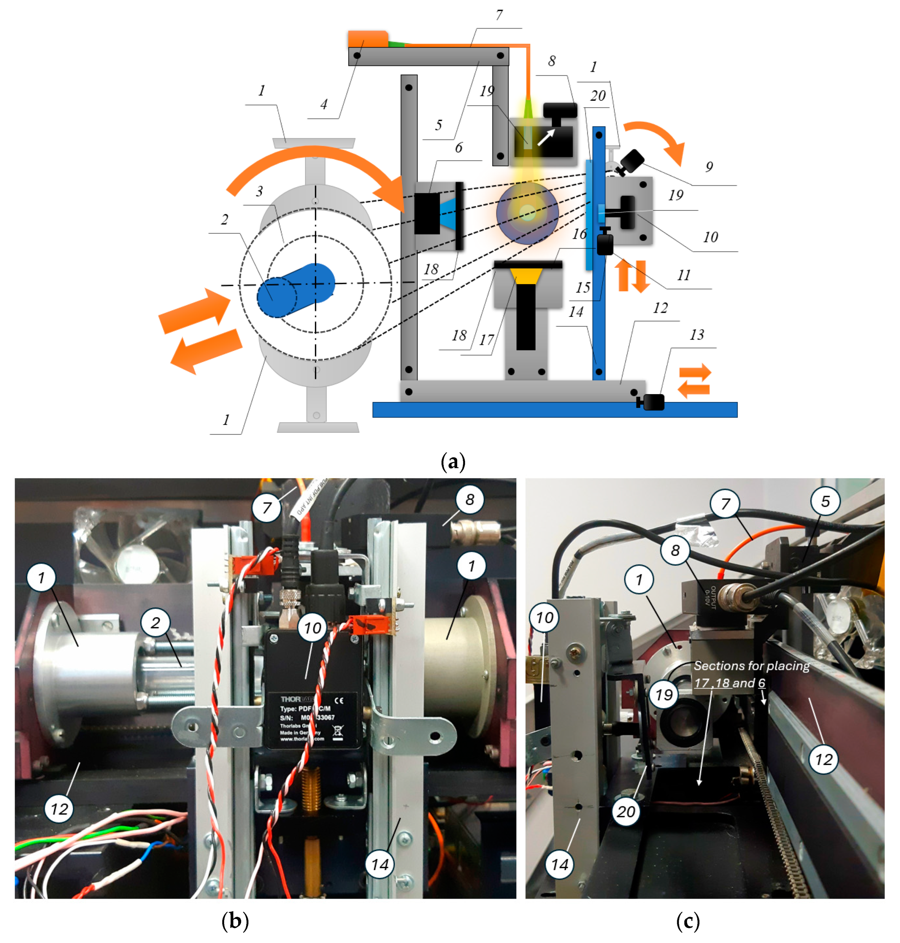
After the preform is installed in the holders, the device lid is closed to prevent reflected or scattered pump radiation from escaping outside—this is a safety requirement when working with the system. The laser diode turns on and operates, allowing measurements to be made at the center point of the reference preform. The system waits until the voltage fluctuations received from both photodetectors (8) and (10) cease to exceed critical values and become acceptable for measurement. Practice has shown that the maximum time for such a wait is about 20 min, and about 7 min on average. The pump radiation is transmitted through a multimode fiber to the collimator and, after passing through the splitter–scatterer (19), enters through the side surface first into the reflective cladding of the optical fiber preform and then into the core, where, among other reagents, active erbium is contained. The active metal begins to luminesce at a wavelength of 1530 nm. It is this radiation that is registered by the detector (10).

After the diode enters the operating mode, the controller gives the motors a command to move the preform so that the pump radiation is directed to the first measurement point. In tomography mode, the rail moves to the zero position and begins translational motion in increments of 50 microns. At each position, the voltages received from photodetectors (10) and (8) are measured with accumulation for 500 ms. This is how the luminescence intensity profile of the active element (erbium and/or ytterbium) is constructed along the diameter of the preform. In the fast-scanning mode, measurements are conducted with the rail moving thanks to a stepper motor (13) from the zero position to the end of the scanning range with a variable step: at the periphery of the cross section, it can reach 400 μm, but, as the rail approaches the core, it decreases to 50 μm. At the point with maximum intensity, the rail stops, and the system performs the same procedure with another stepper motor (11). After the maximum intensity is reached again, the signal is acquired for 1 s. After, a command is given to the longitudinal movement stepper motor (not shown in Figure 1) and the preform moves to the second measurement point. If fast scanning is used, the search area for the core is reduced based on the luminescence profiles in both axes at the previous point, saving time and resources, e.g., elements (11) and (13) and all associated mechanics. If the tomography mode is used, the rail moves to the zero position and scanning begins at a constant step of 50 microns. This continues until the last measurement point is reached. If necessary, the stepper motor (9) performs axial rotation. At each point, the system records the following quantities: voltages received from both photodetectors, the position of motorized positioners for the X coordinate (rail) and Y coordinate (minirails along which the detector (10) moves), laser temperature.

An example of these quantities is shown in Figure 2 and Figure 3.

After receiving the measured values in volts, the pump diode intensity fluctuations are compensated over time using the data obtained by detector (8), and the values of detector (10) are recalculated from the concentration of erbium or ytterbium oxide. For this purpose, the measurement should be obtained during stabilization of the pump diode, when its beam traverses the reference sample, and the photodetector (10) registers the luminescence intensity.

The data obtained by the system was verified using X-ray diffraction analysis (XRDA). To do this, one of the samples with a deliberately created uneven distribution of erbium oxide concentration along its length was divided into fragments, each of which was subjected to XRDA. The correlation coefficient of two dependences of erbium concentration on the coordinate along the length of the preform, obtained by different methods, was 0.98. The fact that the correlation coefficient turned out to be different from 1 can be explained by several factors. Firstly, the reason could be a certain measurement error (possible imperfection of the pump diode intensity fluctuation compensation algorithm); secondly, it is worth noting that XRDA detected all erbium, including clustered one, that is, incapable of luminescence. However, active fibers developers and manufacturers are mainly interested in precisely that erbium that emits radiation at a wavelength of 1.5 microns when pumped at 970–980 nm.

3.2. Preform Geometric Parameters Measurement

It should be noted that already at the stage of luminescent parameters measuring, as mentioned earlier, the XYZ coordinates of the positioners are registered. Since the search algorithms when scanning along both axes find the maximum intensity, this means that the maximum amount of erbium oxide in a given section is concentrated in these areas of the preform. It can be said that a kind of “luminescence geometric center” is being found. Practice has shown that, in most cases, it coincides with the geometric center of the core (which is determined by the refractive index profile). However, in some cases, the geometric center of the core may not correspond to the geometric center of the cladding. Therefore, it is necessary to measure the parameters of the outer surface of the preform. So, after the luminescence features study, the pump diode is turned off and both iris diaphragms are opened. Voltage is applied to the LED and the CCD camera begins to stream the data.

It was previously found that sample side illumination is one of the most effective. Firstly, this brings the problem closer to the already solved one: television measurement of the preform diameter during the chemical vapor deposition process, where the sample is illuminated by the flame of an oxygen–hydrogen torch. Secondly, experiments have shown that face illumination, although possible, is more suitable for the glass surface defects visualization. 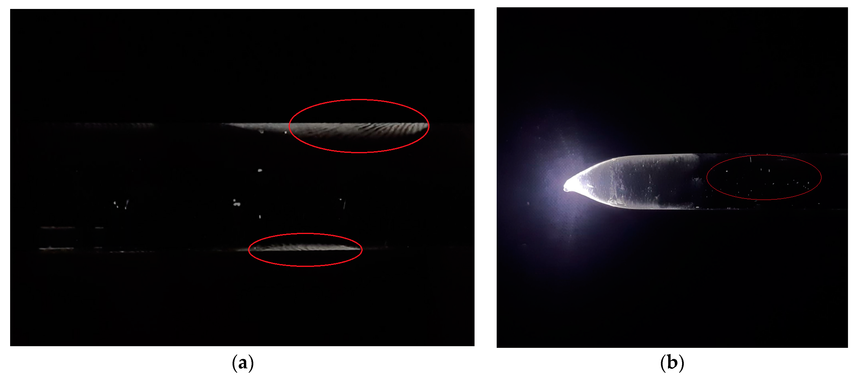Thus, Figure 4 shows a system design variant, where the LED radiation is injected into the technical holder and subsequently propagates along the sample to its opposite end.

In Figure 4a, a human fingerprint is clearly visible, while in Figure 4b there are small scratches (which, of course, according to the optical fiber preforms handling rules, should not exist). In this case, clean preform areas are quite poorly visualized (excluding local narrowings, see figure above). Thus, it is recommended to use side illumination for surface flaw detection. 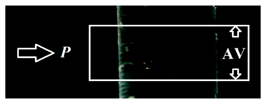An example of side illumination for a preform diameter and center measurement is shown in Figure 5.

In this measurement, the CCD camera captures a rectangular area, which is a raster image containing color information. An area of the preform about 10 mm long is used for averaging (color information is accumulated along the length and then divided by the number of pixels per 10 mm of the preform):

$$I_S=N^{-1}{\displaystyle \sum }_{i=0}^{N-1}{I}_i,$$

(2)

where N is the number of pixels within 10 mm of preform length. Experiments have shown that, for typical preforms with a diameter from 10 mm to 16 mm, it is optimal to select the averaging window in such a way that there are at least 400 pixels per preform diameter. The intensity in the image is also described as [17]:

$$I_S=2^{Q\left(m+2\right)}R+2^{Q\left(m+1\right)}G+2^{Qm}B,$$

(3)

where Q is the bit depth for each color component (R, G, and B), in our case of Q = 8, and m coefficient = 0. Then the R, G, B color components can be obtained as follows:

$$R=\frac{I_s-2^{Q\left(m+1\right)}-I_S\mathrm{mod}{2}^Q}{2^{Q\left(m+2\right)}} ,$$

(4)

$$G=\left[(I_S-I_S\mathrm{mod}{2}^Q)\mathrm{div}{2}^{Q\left(m+1\right)}\right]\mathrm{mod}{2}^{Q\left(m+1\right)},$$

(5)

$$B=I_S\mathrm{mod}{2}^Q,$$

(6)

where ‘div’ and ‘mod’ are the operations that return the result of division with the remainder discarded and the remainder of the division, respectively. Then, the “gray” component is calculated:

$$G{r}_1=\frac{\left(R+G+B\right)}{3},$$

(7)

$$G{r}_2=\frac{\min \left(R,G,B\right)+\max \left(R,G,B\right)}{2},$$

(8)

where Gr₁ and Gr₂ are the two methods for the “gray” component calculation which can be selected depending on the preform illumination type. The profile with the highest contrast among them is selected and assigned to the Gr values. Then, the intensity of the “gray” image is:

$$I_{Gr}=\left(2^{Q\left(m+2\right)}+2^{Q\left(m+1\right)}+2^{Qm}\right)Gr,$$

(9)

The $I_{Gr}$ set of intensities can be visualized as shown in Figure 6.

Ideally, color boundaries can be described by a straight line $H\left(x\right)$ and inverted with the Heaviside function $H^{inv}\left(x\right)$:

$$H\left(x\right)=\left\{\begin{array}{c}0,\hspace{0.33em}x<R\\ 1,\hspace{0.33em}x\ge R\end{array}\right.;\hspace{0.33em}{H}^{inv}\left(x\right)=\left\{\begin{array}{c}1,\hspace{0.33em}x<F\\ 0,\hspace{0.33em}x\ge F\end{array}\right.,$$

(10)

where R and F are coordinates of the leading and trailing edge of the burst (reflection). Straight $H\left(x\right)$ and inverted $H^{inv}\left(x\right)$ Heaviside functions can be represented in continuous form:

$$H\left(x\right) \approx \frac{1}{2}+\frac{1}{2}th\left(kR\right)=\frac{1}{1+e^{-2kR}},$$

(11)

$$H^{inv}\left(x\right) \approx 1-\frac{1}{1+e^{-2kF}},$$

(12)

where k is the “sharpness” of the difference between the zero and one states.

In this case, it seems technically feasible to calculate the correlation coefficient of the obtained data with this function, as well as with functions specified in a table and saved in the system database. Previously, it was shown that calculating the correlation coefficient in a similar way ensures the specified accuracy of localization of layers, including the boundaries of the surface of the fiber light guide preform [18]. However, later, this option was excluded due to the fact that calculating the Pearson’s coefficient in the scanning window loads the system computing resources quite heavily and allows for the result to be obtained only with a delay of 15–30 min, which is quite significant under industrial production conditions.

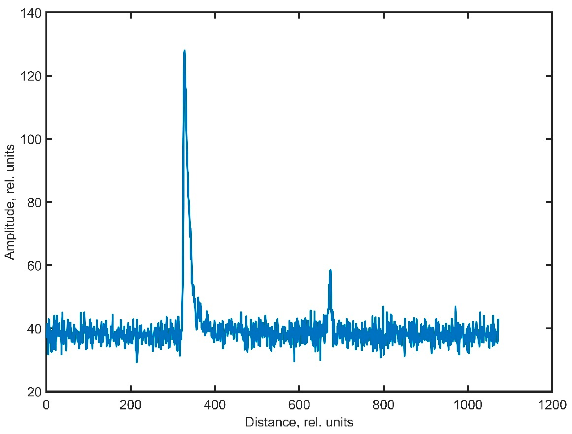
Figure 6 shows that the intensities of the two peaks corresponding to the preform outer layer boundaries are not the same. This is due to the fact that illumination occurs only on one side of the preform under test; therefore, the opposite side of the outer surface is illuminated less intensely. In this regard, with large diameters of the preform, as well as with intense noise during image digitization, mixing of the useful signal (second peak) with noise may take place. There are several ways to get rid of the noise component:

• Expanding the area where the preform is captured by the CCD camera and, as a result, obtaining more data for accumulation, thereby increasing the signal-to-noise ratio (SNR) of the data entering the system. This solution seems to be the most obvious; however, it requires an increase in the distance between the camera and the sample under test and, as a consequence, an increase in the dimensions of the product. This is unacceptable since the system is already quite large. In addition, the spatial resolution of the method will decrease;
• Increased data accumulation time. This measure will also lead to an increase in the SNR, although at the cost of the technological process lengthening;
• Digital signal processing. A method was recently presented that can increase the signal-to-noise ratio by more than 10 dB when using optical sensors. The ability to do so lies in the fact that a one-dimensional discretely specified array of real or integer data can be processed in such a way that their various components can be either averaged or left unchanged according to a specially defined law. In the simplest case, this may be a law that describes the dependence of the averaging parameter (for example, the size of the scanning window) on the signal parameter (suppose its intensity at a particular frequency or in a certain spatial coordinate).

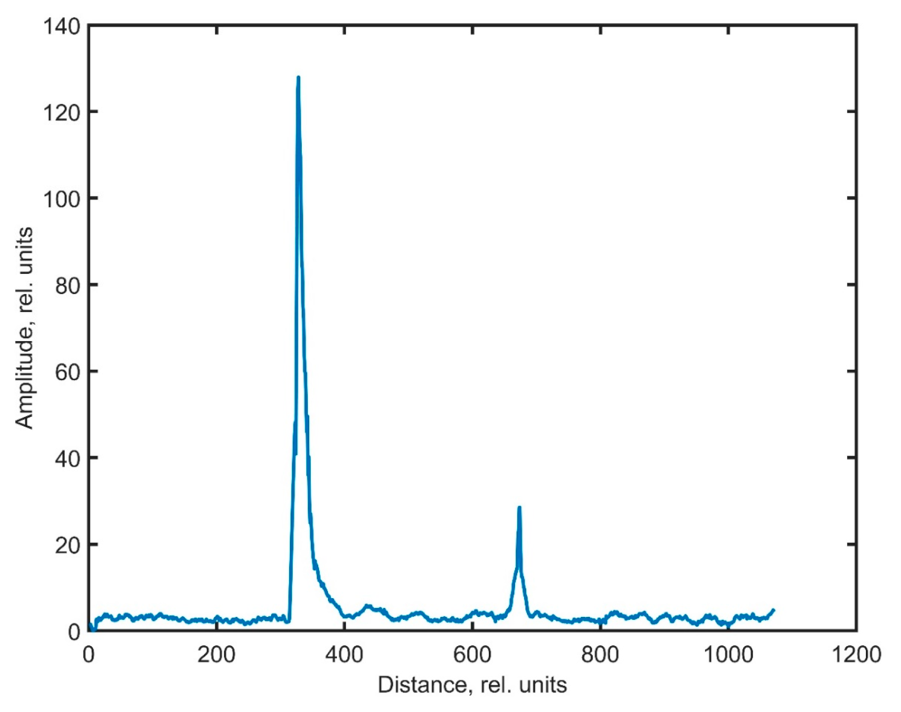
Thus, Figure 7 shows the result of the obtained noisy data processing using the activation function dynamic averaging (AFDA) method [19]. This is an improved algorithm based on the frequency domain dynamic averaging (FDDA) technique, which was originally created for optical frequency domain reflectometers and coherent optical time domain reflectometers data processing [20].

The AFDA/FDDA techniques are based on the following approach. First, all values in an I_(j) array of N elements are normalized from 0 to 1. After this, the I_a(j) filtered array is written [21]:

$$i-\frac{w_j}{2}\ge 0;\hspace{0.33em}i-\frac{w_j}{2}<N,$$

(13)

$$I_{a\left(j\right)}=\frac{1}{w_j}{\displaystyle \sum }_{i-\frac{w_j}{2}}^{i+\frac{w_j}{2}}{P}_i,$$

(14)

$$w_j=w^{\prime }\left(1-I_{\left(j\right)}\right),$$

(15)

where I_a(j) stands for filtered signal, j is the pixel number, $w^{\prime }$ is the maximum event (burst) size in pixels.

The noise distribution of detectors that register backscattering in reflectometers is similar to the noise of the photosensitive elements of video cameras—this can be concluded by comparing the histograms presented in [22,23]. The useful signal, just as in the works above, is a sharp “outburst”. This means that FDDA-like approaches can also work for the data types studied in this work. Obviously, Equation (15) describes the linear function $w_j=f\left(I_{\left(j\right)}\right)$. It has been shown that the choice of a linear function is not always appropriate in this case [18]. In this work, Turov et al. justify the use of the GELU function (neuron activation function described by Gaussian Error Linear Unit) [24]. 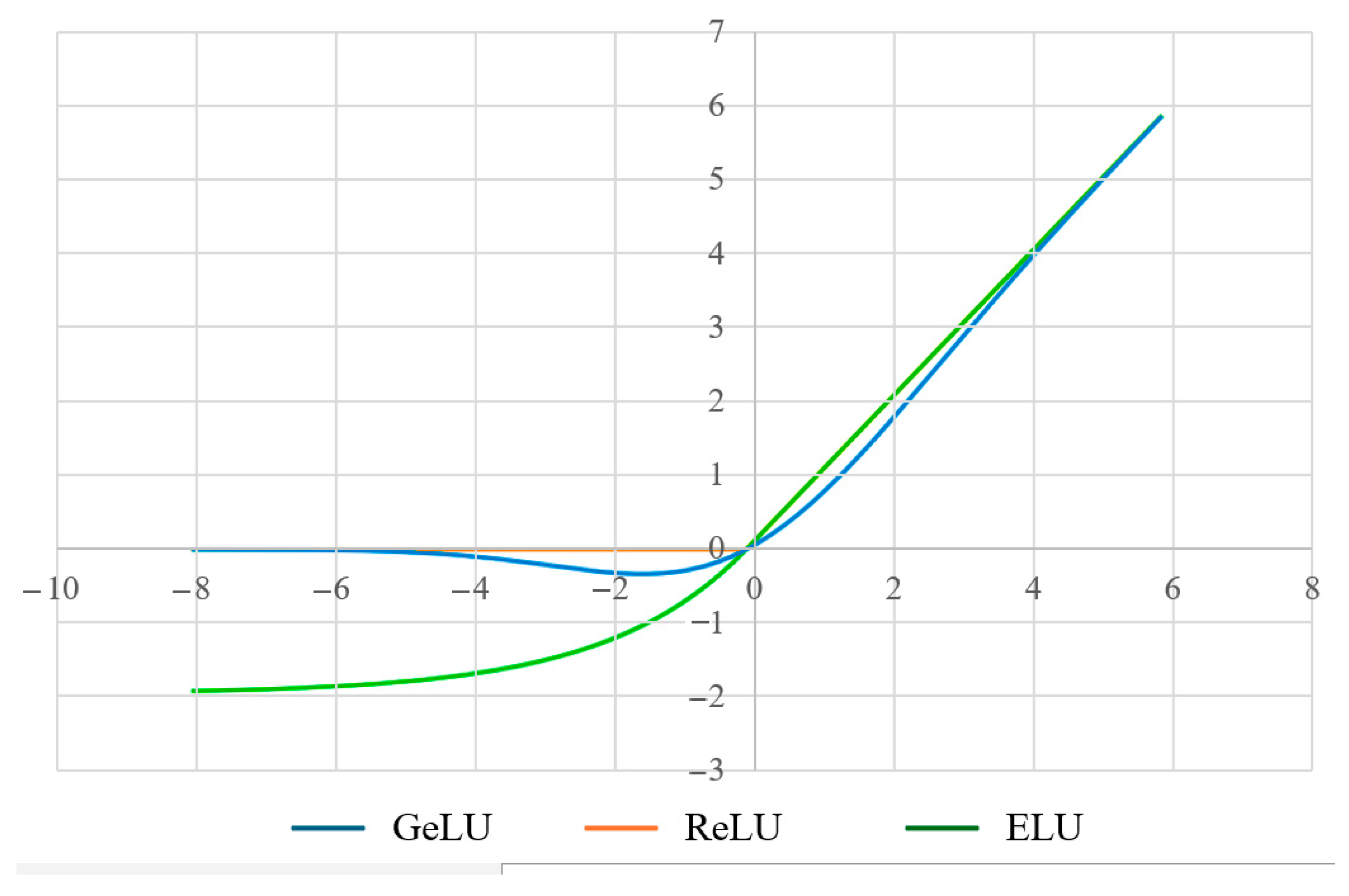Of course, [19] allows one to assume that the features leading to the choice of the GELU function as a characteristic of a digital filter processing data from reflectometers of various types, owing to the similarity of the data, can be projected onto the preform external borders identifying problems. However, it is necessary to note a number of its advantages over others—precisely for conducting the research described in this work. Thus, below, other neuron activation functions are presented analytically (16)–(19) and graphically (Figure 8) [24]. Of all these expressions, the GELU function is the most flexible and suitable for the problem. The reasons are described below.

Rectified Linear Units (ReLU) is a type of activation function that grows linearly when the argument is positive but is zero when the argument is negative. The kink of this function ensures the nonlinearity of its response:

$$w_j=0\mathrm{when} I_{\left(j\right)}\le B;w_j=I_{\left(j\right)}\mathrm{when} I_{\left(j\right)}>B,$$

(16)

where B is the kink point (which can occur not only at zero, but at any other position). Essentially, the use of this activation function for dynamic averaging and noise filtering is a combination of the FDDA method and a threshold algorithm, as demonstrated in [19]. Fairly high processed signal SNR values were obtained in it. However, the filtered useful signal had a number of disadvantages. New distortions were introduced, some of which were associated with edge effects, and some with the incorrect choice of function (in particular, presumably, with the presence of an obvious kink point). The exponential linear unit (ELU) function does not have such problems [25]:

$$w_j=I_{\left(j\right)} \mathrm{when} I_{\left(j\right)}\le B;w_j=(e^{I_{\left(j\right)} }-1)\alpha \mathrm{when} I_{\left(j\right)}>B,$$

(17)

where α > 0 and B is the coordinate where the exponential and the straight line intersect.

However, this activation function divides the signal intensity region into only two zones, determined by the parameters B and α, which may not be enough for flexible adjustment of the filtering function. Therefore, as in [19], it is proposed to use an inverted GELU function combined with another exponential instead:

$$w_j=-0.5I_{\left(j\right) }\left[1+\frac{2}{\sqrt{\pi }}{{\displaystyle \int }}_0^{\frac{I_{\left(j\right)}}{\sqrt{2}}}{e}^{-t^2}dt\right]\mathrm{when} I_{\left(j\right) }<B;$$

(18)

$$w_j={\left(1+e^{-3y+C}\right)}^{-1}\mathrm{when} I_{\left(j\right) }\ge B,$$

(19)

where y and C are the adjustment parameters of the filtering function. It is known that the resulting function can be approximated, to some extent, by the logistic activation function (sigmoidal), and its GELU component can be simplified to:

$$w_j=0.5I_{\left(j\right) }\left[\sqrt{\frac{2}{\pi }}\left(I_{\left(j\right) }+0.044715x^3\right)\right]$$

(20)

However, according to [26], this does not provide a significant gain in computing resources consumption, and also deprives the function of a large number of tuning coefficients.

Before dynamic filtering, binary and threshold filters can be applied to each original image row instead of the averaged one. The image is converted to binary with a T threshold: if the pixel brightness is less than T, then it is equal to 0, otherwise it is equal to 1. After this, a threshold filter is applied to eliminate events containing less than k pixels. The image is then averaged and subjected to AFDA. 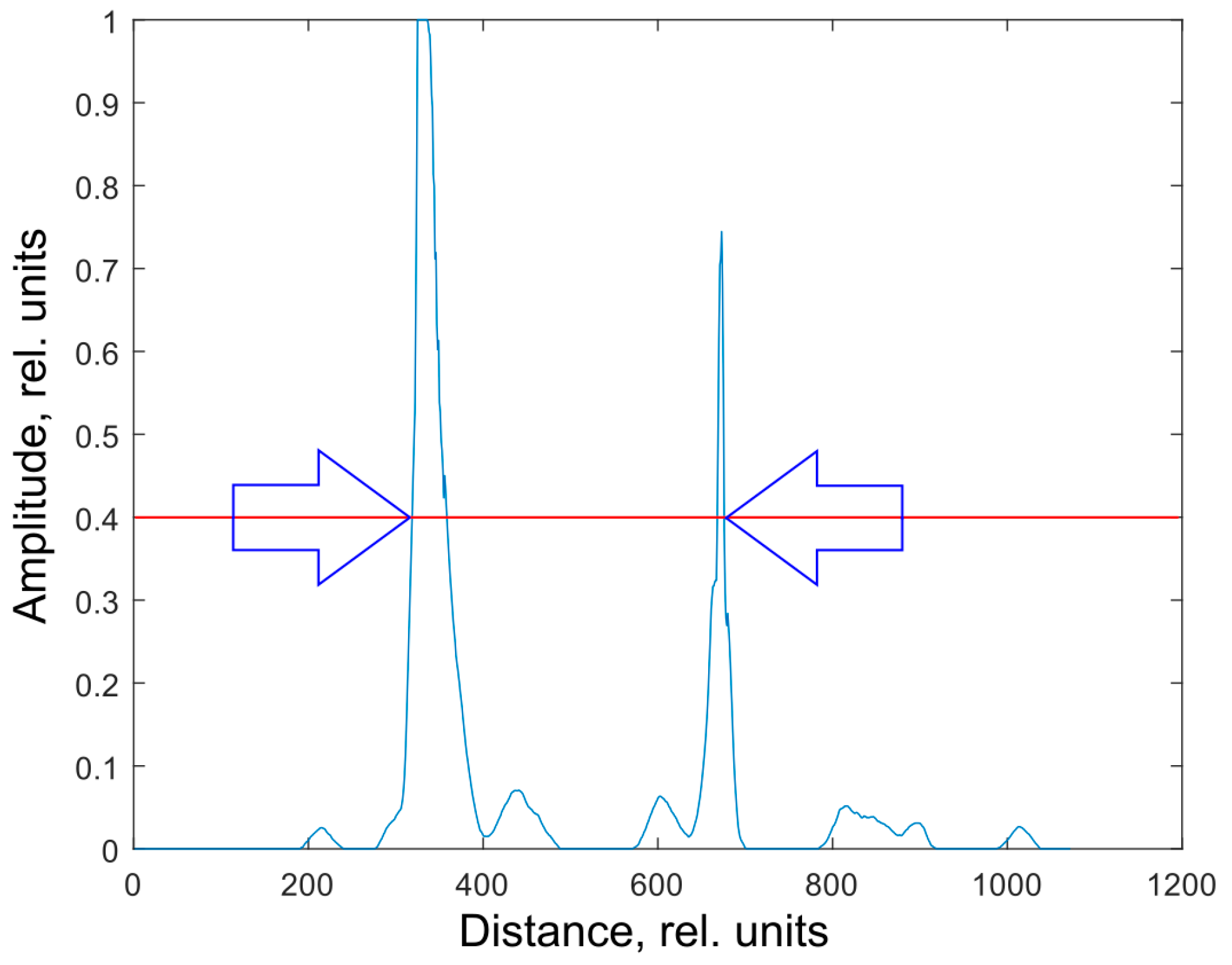The output data for k = 180 and T = 15 are presented in Figure 9.

It can be seen from the figure that the leading edge of the first event and the trailing edge of the second are represented by the lines almost perpendicular to the abscissa axis. The experiment showed that their strict perpendicularity is occasionally violated only by a line displacement of 1 pixel, which, with a preform diameter of about 10 mm, is 12–25 microns (depending on the focal length of the camera). This accuracy is enough to detect defects at an early stage. After the boundaries of the outer layer are determined from the event edges, the geometric center of the preform is calculated at the location where the measurement takes place:

C = 0.5 (F_b + F_a) K,

(21)

where F_a is the coordinate of the leading edge of the first event, F_b is the coordinate of the trailing edge of the second event, K is the conversion factor from pixels to SI length units.

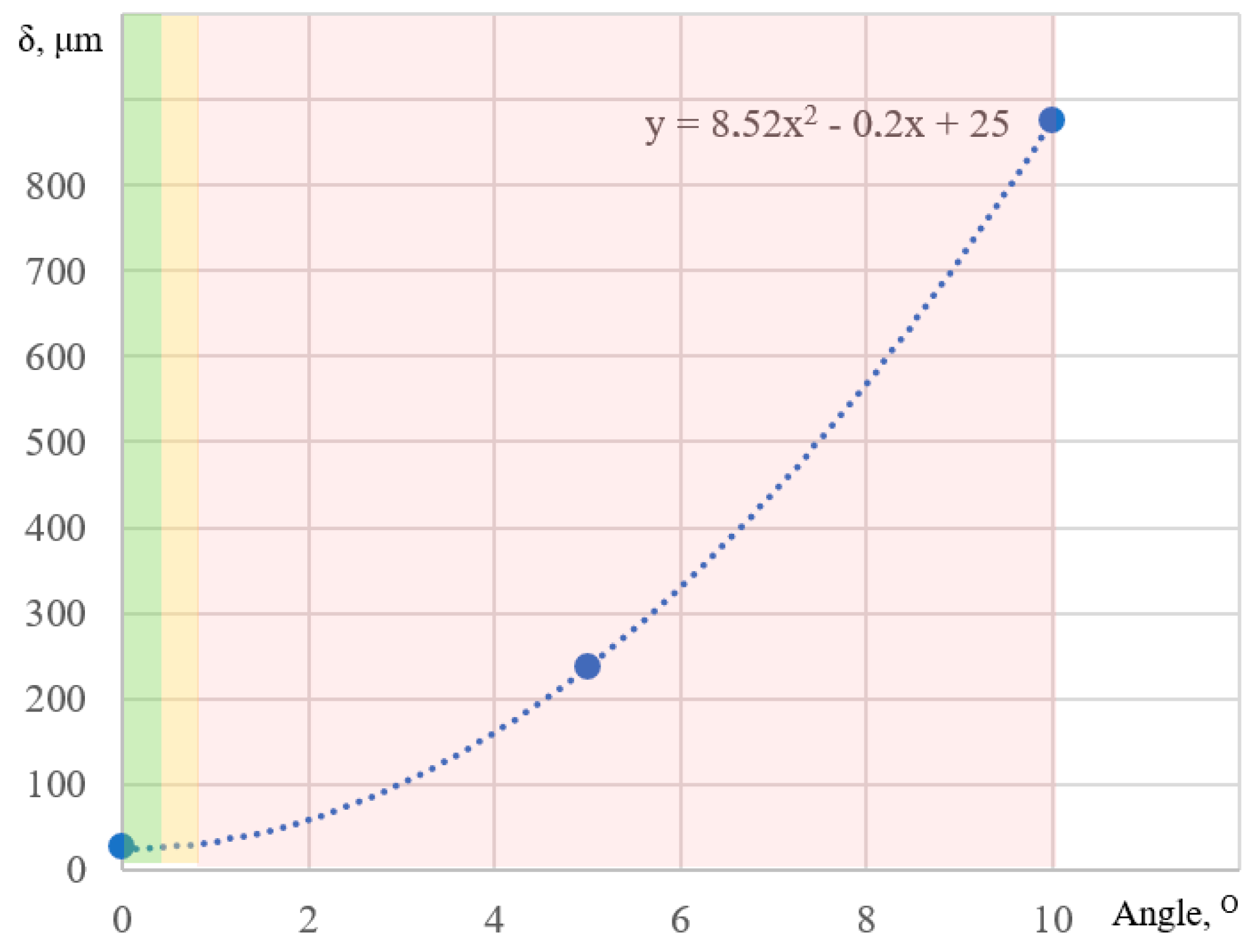
It is worth noting, however, that the sample geometric center detecting accuracy at the location under testing deteriorates with the increasing sample cylindricity deviation. This is due to the fact that, during the tilted preform image averaging, the lines of a two-dimensional array containing information about the boundaries are shifted relative to each other and this gives rise to the edge “blurring”. 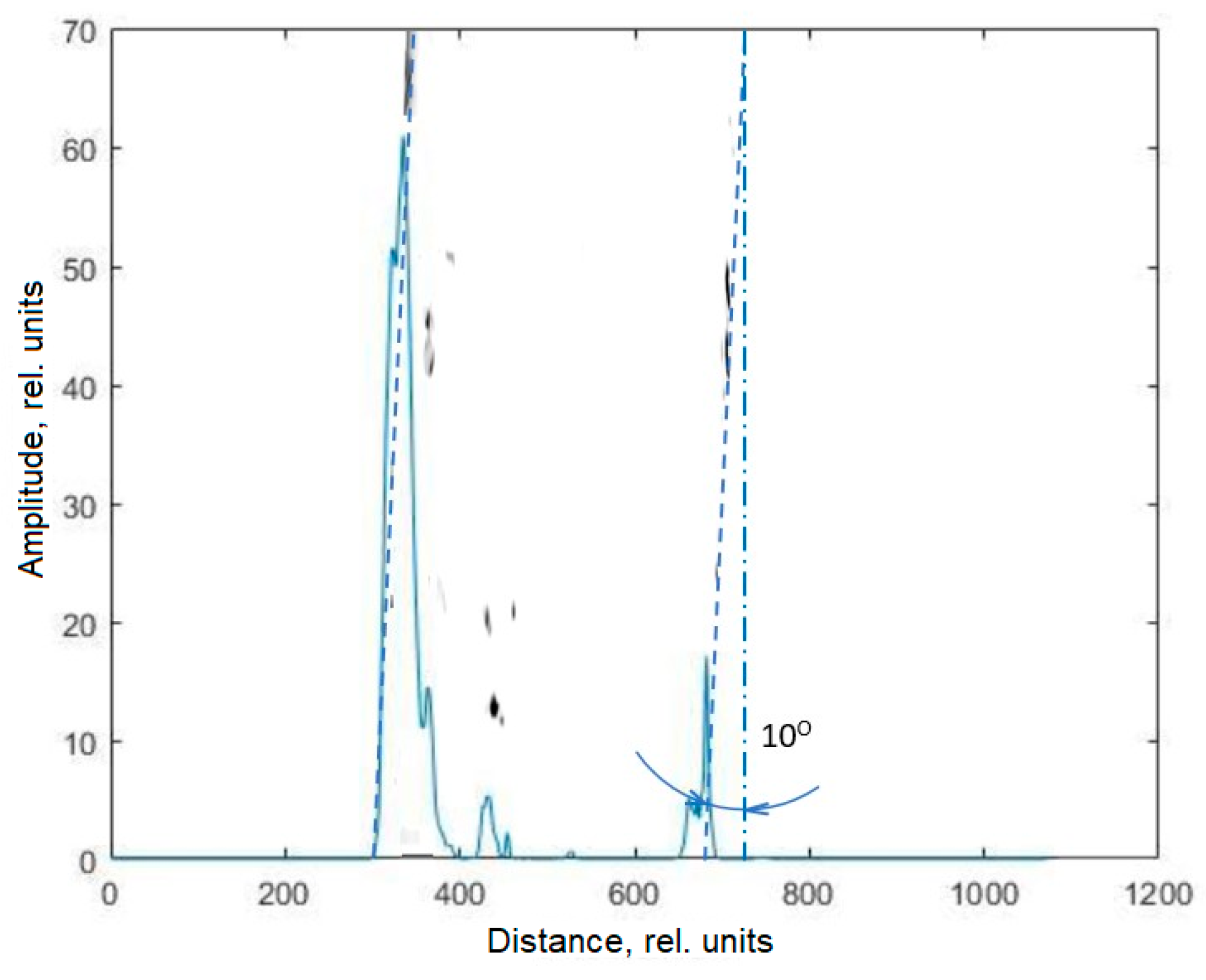This can be seen quite clearly from Figure 10.

Figure 10, which also overlays the inverted color image from the camera (as well as dotted lines highlighting the boundaries), shows the extreme cylindricity deviation when the preform is rotated 10° relative to the camera. This practically unrealistic case will result in a measurement error of up to 850 µm; a deviation of 5° will result in an error of up to 240 µm. Real deviations rarely exceed 0.25°. The figure shows that, with such deviations, the inaccuracy of preform boundaries or geometric center detecting does not exceed 30 μm (Figure 11).

It can be seen from the figures that, when the preform is rotated, the width of the events increases. That is why the width of both peaks at half maximum is additionally calculated. If, for some reason, the peak edges were not steep enough to obtain correct data, then this indicator value warns of a possible drop in the measurement accuracy in a particular location.

3.3. Refractive Index Profile Stability Monitoring

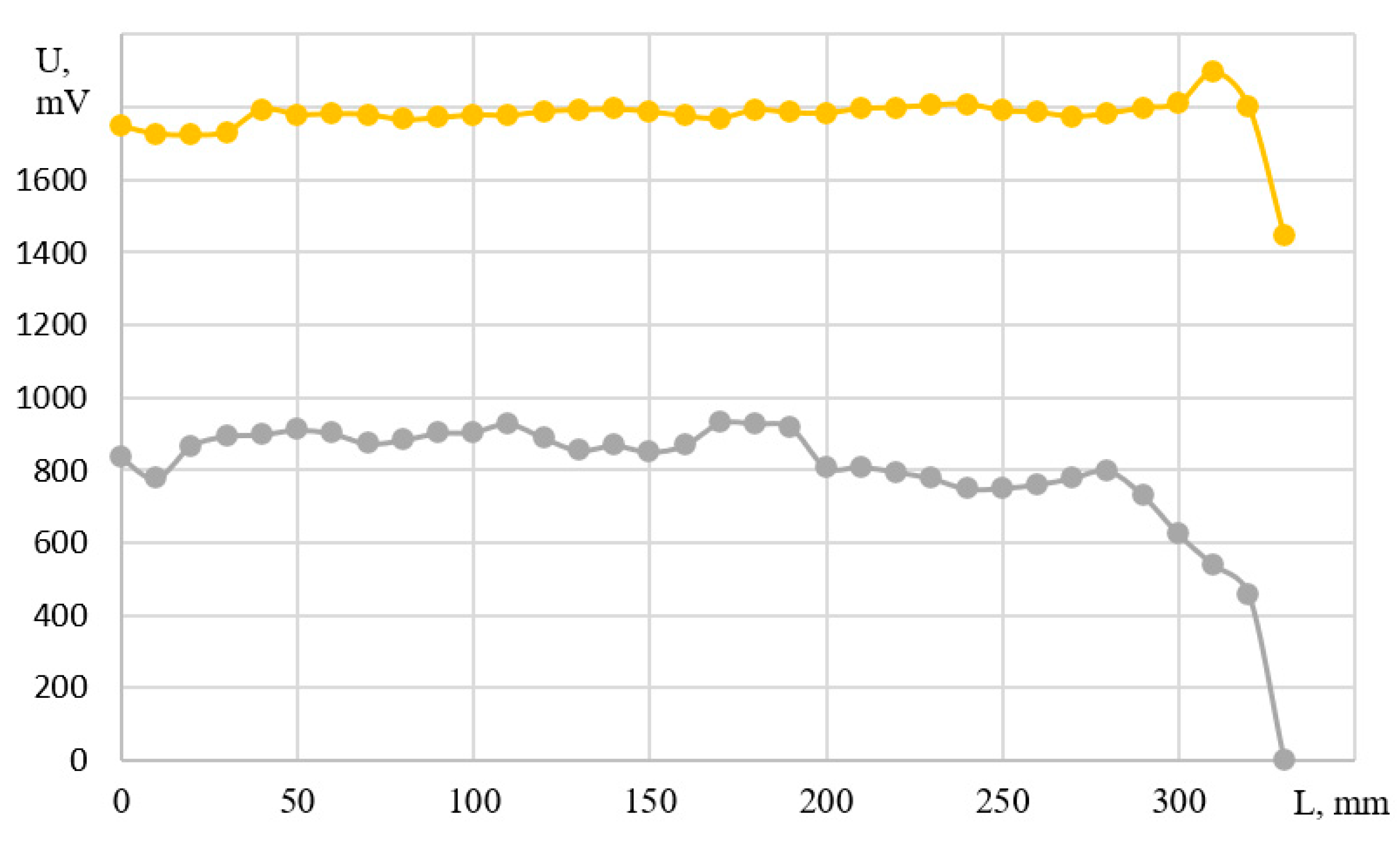
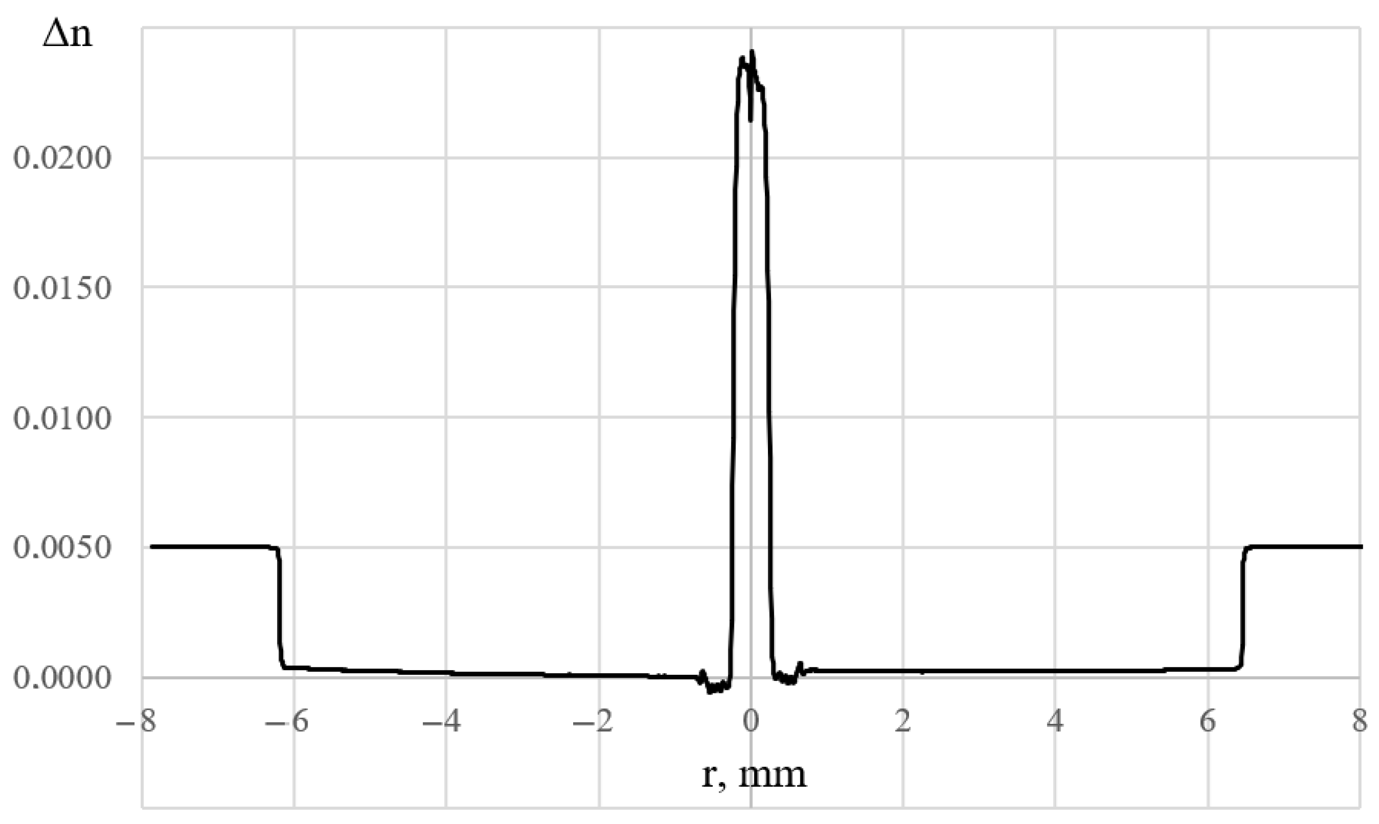
The distribution of optical–geometric characteristics along the length of the optical fiber is determined by the stability of the refractive-index–preform radius function in each position and projection. To save time in the overall process, detailed examination of the refractive index profile can be carried out using special equipment in one position of the preform. Figure 12, for example, illustrates the refractive index profile of a silicon oxide, germanium oxide, aluminum oxide, and erbium oxide doped preform, obtained using a commercial testing setup PK2600 (Photon Kinetics, Beaverton, OR, USA).

Unlike the PK2600 setup, the proposed system uses a simple white light source instead of a red laser scanning over the cross section of the preform. The rays emerging from it pass at different angles and different points through the preform; therefore, what the CCD camera records is not the deflection function of any individual ray, but a certain integral dependence common to all these individual trajectories of light and unique for each section.

The measurement operates as follows. An aluminum plate, which is fixed to the side of the optical filter and a few centimeters from the beam of the pump diode, has a color code printed on its surface using heat-resistant paint—this is similar to a QR code, consisting of different areas. For measurement, the camera, radiation source, and sample may not be in a straight line because the white light diode in a multi-reflective measurement cell acts almost as an omnidirectional source. Reflecting from the color-coded plate, light passes through the preform and creates a color pattern on its side surface. This pattern I′ is captured by the camera and converted into a one-dimensional array using the formula:

$$D_j=po{s}_{max}\left|I_{\left(i+1,j\right)}^{\prime }-I_{\left(i,j\right)}^{\prime }\right|d^{-1},$$

(22)

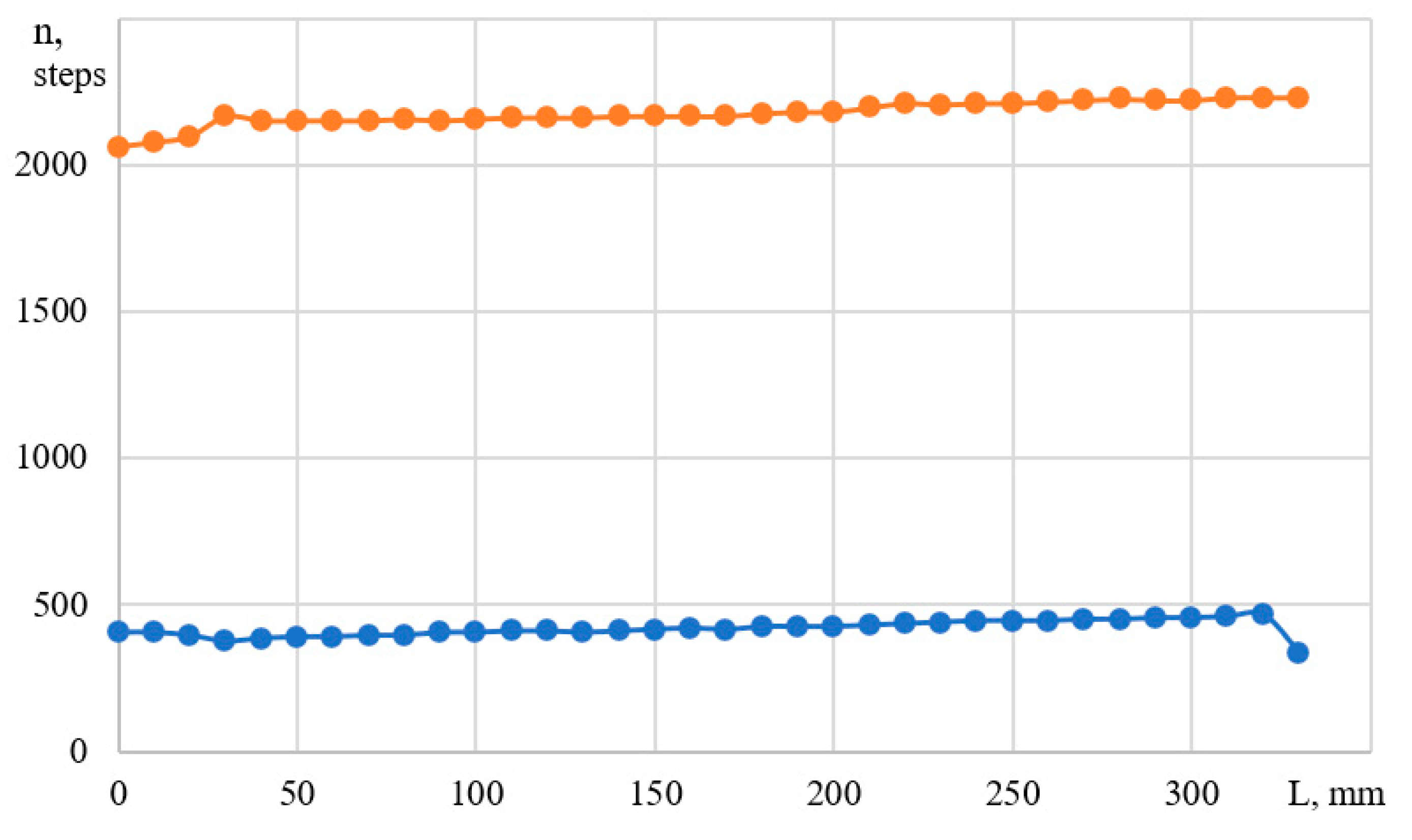
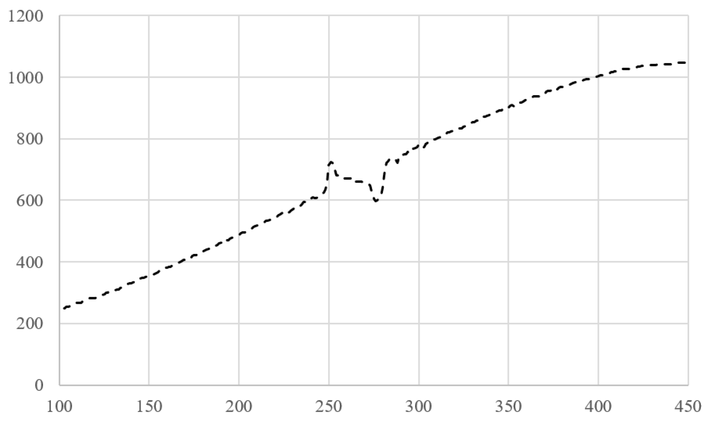
where pos_max returns the peak coordinate in pixels and d is a derivative step. The D_j dependence is presented in Figure 13. It is easy to see that, visually, it resembles the deflection function obtained by typical preform analyzers. We call this function ‘integral’ because it is obtained by the interaction of a large number of rays reflected at different angles, as mentioned above.

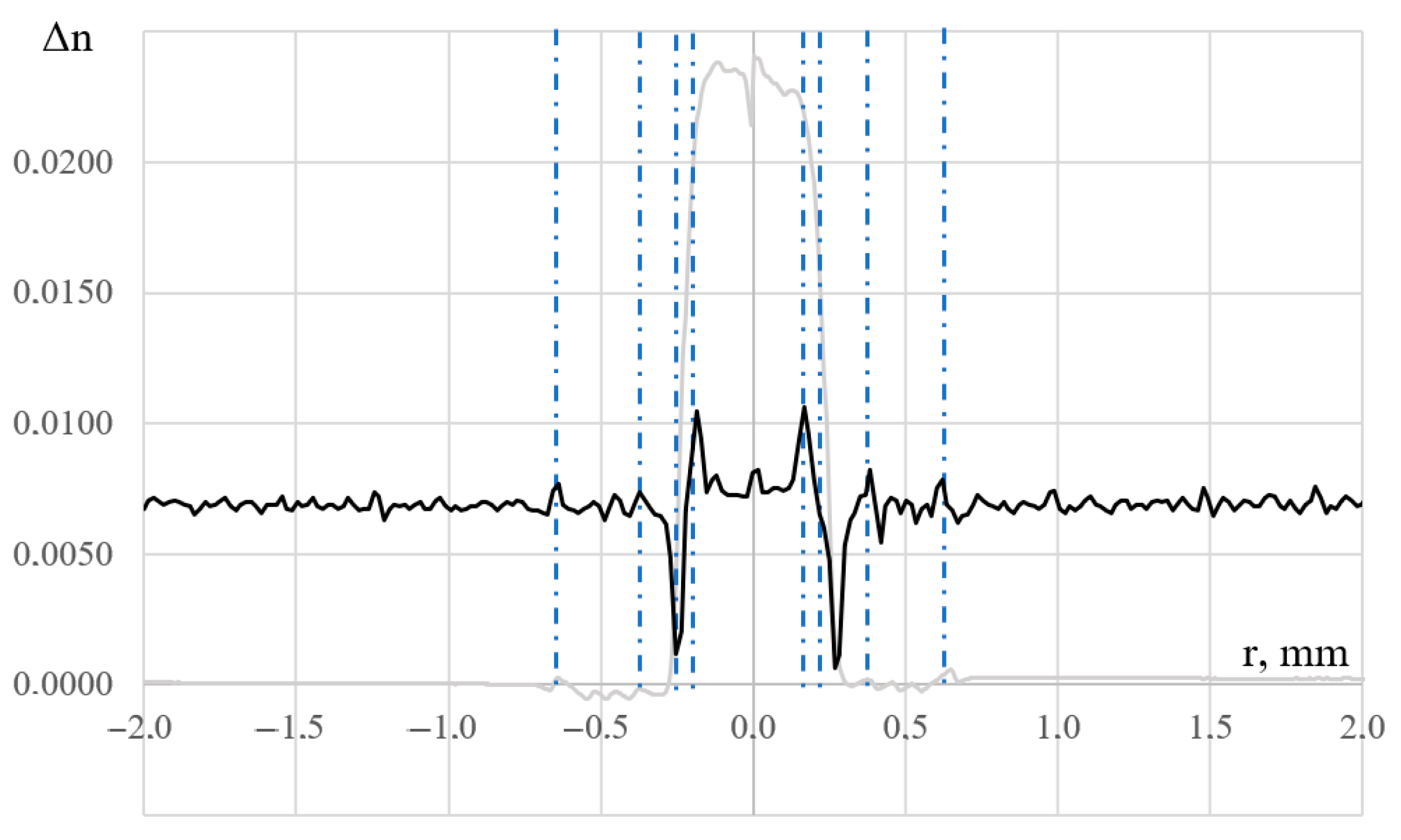
However, in the future, it is proposed to operate with the modulus of its derivative (with respect to the spatial coordinate), since the integral deflection function itself contains an undesirable large bend, against the background of which small changes in the refractive index are not very noticeable (Figure 14). This function could be expressed as:

$$D_j^{\prime }=\left|D_{j+\Delta }-D_j\right|{\Delta }^{-1}$$

(23)

Part of the previous one is superimposed on this figure to give a visual representation of the events (layer boundaries) having some relationship with the refractive index profile obtained with the PK2600. Unfortunately, the resulting function, unlike the standard deviation function in a preform analyzer, cannot be converted into a refractive index profile due to the large number of unknown parameters. However, since it is possible to obtain this function in any position of the preform, using correlation analysis it is possible to compare this function in each position with a “reference” function previously stored in the device memory. Such a standard must be stored for each type of optical fiber preform. Of course, it is quite difficult to produce two or more identical preforms, but production always requires an increase in the suitable products percentage. The reference does not contain a refractive index profile in the classical sense: it contains information about the boundaries of the sample layers. This can be compared to the settings file of a typical refractive index profile analyzer, which stores the search area for layer boundaries. Of course, it is almost impossible to achieve a correlation coefficient of 1 between the test sample and the reference; therefore, the user must set the required threshold value based on the conditions imposed by the preform manufacturer. If the function u obtained in the form of a discrete one-dimensional array is compared to the reference function v, the correlation coefficient between them, R, will be written as [27]:

$$R={\displaystyle \sum }_{i=0}^n\left(u_i-〈u〉\right)\left(v_i-〈v〉\right){\left[{\displaystyle \sum }_{i=0}^n{\left(u_i-〈u〉\right)}^2{\displaystyle \sum }_{i=0}^n{\left(v_i-〈v〉\right)}^2\right]}^{-\frac{1}{2}},$$

(24)

where < > means the average value.

Initially, the value of R_min is entered into the system, which is in the range of −1 to 1. If all correlation coefficients calculated for each section have a value of R > R_min, the preform is recognized as the one having acceptable quality and proceeds to further stages of production. Otherwise, it is subjected to additional tests using a refractive index profile analyzer.

4. Discussion

Data characterizing the quality and accuracy of certain physical quantity measurements using the system presented in this work are given in

Table 1. Presented techniques features and accuracy.

Measurement Type	Accuracy
Erbium oxide concentration distribution	Accuracy along the sample: 1 mm; 0.2 dB/m with the dynamic range of 50 dB/m (in units of rare earth metal absorption in the drawn fiber)
Diameter and geometric center coordinate measurement	12–25 µm
Refractive index profile	(Indicator measurement)

.

When studying the active erbium ions concentration distribution in an optical fiber preform, a sufficiently high dynamic range was obtained, making it possible to measure not only erbium, but also ytterbium preforms. Since the data obtained are often compared with the absorption loss of erbium in a specific type of optical fiber, it will be convenient to say that the dynamic range allows one to measure preforms from which fibers will be drawn with an absorption loss coefficient of the optical signal in the region of 980 nm, not exceeding 50 dB/m, and with an accuracy of 0.2 dB/m. The accuracy of surface boundary allocation in the absence of gross cylindricity deviations is determined by the type of camera, its distance to the sample, the correctness of the illumination, and by whether it is in the range of 12–25 microns. The quality of the refractive index profile uniformity test along the preform is more difficult to assess. Firstly, it will also be determined by the pitch of the photodetector matrix. Secondly, the multi-beam nature of light in the study area forms the so-called integral deflection function, which is quite difficult to recalculate into a metrologically correct refractive index profile as is done in serial analyzers. However, by assessing the correlation between the integral deflection function at each point and the reference array formed for each type of fiber preform, it is possible to qualitatively assess the uniformity of the optical–geometric characteristics. This type of research can be classified as an indicator measurement method.

Practice has shown that the data obtained make it possible to flexibly control the technological process of producing active optical fibers, as well as save raw materials and semi-finished products, while reducing the duration of the technological process.

As a future work, it will be appropriate to consider the possibility of an aluminum oxide concentration study, as aluminum is one of the most important components in the active optical fiber preform. Theoretically, it can be studied using the photofluorescent method, pumping aluminum ions with a xenon lamp and reading the useful signal with a detector sensitive to radiation at the edge of the ultraviolet and visible ranges [28]. However, such a hardware complication of the system presented in this work can lead to a significant complication of operating regimes and an increase in the technological process duration. So, in the future, it is proposed to utilize the MCVD method preform production features. The final stage of the process is the so-called collapse, in which part of the deposited germanium oxide evaporates from the central region of the preform subject to high temperatures and the refractive index profile gets a kind of “dip”, with a refractive index independent of the germanium concentration (Figure 15).

Then, the level of the bottom part of this “dip” will be determined mostly by the influence of aluminum oxide on the refractive index in the location under testing. It is easy to notice that the resulting integral deflection function also has an event in the central part of the sample. The size of this burst (D₂) is closely related to the size of D₁. Of course, taking into account the fact that the process is also contributed to by the possible collapse mode non-reproducibility, the core refractive index instability, the difficulty of recording the deflection function at its center, as well as the presence of an obvious but so far undescribed connection of events (layer boundaries) on the integral deflection function and refractive index profile, there is no need to talk about a full measurement of the aluminum oxide concentration along the preform. This approach will result rather in an indicator study of aluminum oxide. If D₂ increases, then the concentration of aluminum oxide is most likely higher than in the previous position; if, on the contrary, it decreases, then there is less aluminum oxide in this position.

5. Conclusions and Future Work

In this work, the measurement of the optical, geometric, and luminescent properties of a preform within a single automated laboratory bench was described. All processes are highly automated and provide distributed research of the required physical quantities. The study of the refractive index profile variations along the length of the preform is carried out without immersing the preform in synthetic oil, making the process less labor-intensive and safer. It was shown that the study of the erbium oxide concentration in the active form, the evolution of the refractive index profile along the length, as well as the geometric parameters of the preform can be carried out not in a sequential mode, but in a parallel one.

For all distributed measurements made on this instrument, a spatial resolution of 1 mm is valid. According to XRDA, the error in measuring the concentration of active erbium is no more than 5%, and a significant portion of this error is explained by the fact that the XRDA method also detects clustered erbium. In already drawn fibers, the content of active erbium is estimated by absorption losses in the region of 980 nm. According to preliminary estimates, it is about 0.2 dB/m; however, to obtain a more accurate value, it is necessary to carry out a long collection of statistics. This is a future task for our scientific group.

Another important upcoming task is the variation of system component parameters. The diode, having a spectrum similar to that presented in [29] which is used to illuminate preforms, can be replaced with other radiation sources, while the accuracy of sample boundary determination, as well as the integral deviation function, should be studied.

It is also necessary to conduct research to reconstruct the full refractive index profile from the integral deflection function. Since it is quite difficult to establish an analytical relationship between these two functions, it is advisable to use artificial intelligence algorithms in the future [30,31].

References

1. Abdhul Rahuman, M.A.; Kahatapitiya, N.S.; Amarakoon, V.N.; Wijenayake, U.; Silva, B.N.; Jeon, M.; Kim, J.; Ravichandran, N.K.; Wijesinghe, R.E. Recent Technological Progress of Fiber-Optical Sensors for Bio-Mechatronics Applications. Technologies 2023, 11, 157. [Google Scholar] [CrossRef]
2. Kim, T.H. Analysis of Optical Communications, Fiber Optics, Sensors and Laser Applications. J. Mach. Comput. 2023, 3, 115–125. [Google Scholar] [CrossRef]
3. Matveenko, V.; Serovaev, G. Distributed Strain Measurements Based on Rayleigh Scattering in the Presence of Fiber Bragg Gratings in an Optical Fiber. Photonics 2023, 10, 868. [Google Scholar] [CrossRef]
4. Zhirnov, A.A.; Choban, T.V.; Stepanov, K.V.; Koshelev, K.I.; Chernutsky, A.O.; Pnev, A.B.; Karasik, V.E. Distributed acoustic sensor using a double Sagnac interferometer based on wavelength division multiplexing. Sensors 2022, 22, 2772. [Google Scholar] [CrossRef]
5. Bogachkov, I.V. Creation of Adaptive Algorithms for Determining the Brillouin Frequency Shift and Tension of Optical Fiber. Instrum. Exp. Tech. 2023, 66, 769–774. [Google Scholar] [CrossRef]
6. Aksenov, V.A.; Ivanov, G.A.; Iskhakova, L.D.; Likhachev, M.E.; Chernook, S.G.; Shushpanov, O.E. Properties of fluorosilicate glass prepared by MCVD. Inorg. Mater. 2010, 46, 1151–1154. [Google Scholar] [CrossRef]
7. Yassin, S.M.; Omar, N.Y.M.; Abdul-Rashid, H.A. Optimized fabrication of thulium doped silica optical fiber using MCVD. In Handbook of Optical Fibers; Springer: Berlin/Heidelberg, Germany, 2018; pp. 1–35. [Google Scholar]
8. Cieslikiewicz-Bouet, M.; El Hamzaoui, H.; Ouerdane, Y.; Mahiou, R.; Chadeyron, G.; Bigot, L.; Delplace-Baudelle, K.; Habert, R.; Plus, S.; Cassez, A.; et al. Investigation of the incorporation of cerium ions in MCVD-silica glass preforms for remote optical fiber radiation dosimetry. Sensors 2021, 21, 3362. [Google Scholar] [CrossRef]
9. Saekeang, C.; Chu, P.L.; Whitbread, T.W. Nondestructive measurement of refractive-index profile and cross-sectional geometry of optical fiber preforms. Appl. Opt. 1980, 19, 2025–2030. [Google Scholar] [CrossRef] [PubMed]
10. Kokubun, Y.; Iga, K. Refractive-index profile measurement of preform rods by a transverse differential interferogram. Appl. Opt. 1980, 19, 846–851. [Google Scholar] [CrossRef] [PubMed]
11. Glantschnig, W. How accurately can one reconstruct an index profile from transverse measurement data? J. Light. Technol. 1985, 3, 678–683. [Google Scholar] [CrossRef]
12. Latkin, K. The simulation of active ions luminescence in the preform core under the pumping through the lateral surface. Opt. Commun. 2023, 542, 129564. [Google Scholar] [CrossRef]
13. Vivona, M.; Zervas, M.N. Full non-destructive characterization of doped optical fiber preforms. In Fiber Lasers XVI: Technology and Systems; SPIE: Bellingham, WA, USA, 2019; Volume 10897, pp. 40–45. [Google Scholar]
14. Vivona, M.; Zervas, M.N. Instrumentation for simultaneous non-destructive profiling of refractive index and rare-earth-ion distributions in optical fiber preforms. Instruments 2018, 2, 23. [Google Scholar] [CrossRef]
15. Vivona, M.; Kim, J.; Zervas, M.N. Non-destructive characterization of rare-earth-doped optical fiber preforms. Opt. Lett. 2018, 43, 4907–4910. [Google Scholar] [CrossRef] [PubMed]
16. Matějec, V.; Kašík, I.; Berková, D.; Hayer, M.; Chomát, M.; Berka, Z.; Langrová, A. Properties of optical fiber preforms prepared by inner coating of substrate tubes. Ceram-Silik 2001, 45, 62–69. [Google Scholar]
17. RGB Color Codes Table. RT Online Calculators and Instruments. Available online: https://www.rapidtables.org/ru/web/color/RGB_Color.html (accessed on 18 October 2023).
18. Konstantinov, Y.A. Automation of Technical Quality Assessment Processes for Special Fiber Light Guides at Production Stages. Ph.D. Thesis, Perm National Research Polytechnic University, Perm, Russia, 2012. [Google Scholar]
19. Turov, A.T.; Barkov, F.L.; Konstantinov, Y.A.; Korobko, D.A.; Lopez-Mercado, C.A.; Fotiadi, A.A. Activation Function Dynamic Averaging as a Technique for Nonlinear 2D Data Denoising in Distributed Acoustic Sensors. Algorithms 2023, 16, 440. [Google Scholar] [CrossRef]
20. Turov, A.T.; Konstantinov, Y.A.; Barkov, F.L.; Korobko, D.A.; Zolotovskii, I.O.; Lopez-Mercado, C.A.; Fotiadi, A.A. Enhancing the Distributed Acoustic Sensors’(DAS) Performance by the Simple Noise Reduction Algorithms Sequential Application. Algorithms 2023, 16, 217. [Google Scholar] [CrossRef]
21. Ponomarev, R.S.; Konstantinov, Y.A.; Belokrylov, M.E.; Shevtsov, D.I.; Karnaushkin, P.V. An Automated Instrument for Reflectometry Study of the Pyroelectric Effect in Proton-Exchange Channel Waveguides Based on Lithium Niobate. Instrum. Exp. Tech. 2022, 65, 787–796. [Google Scholar] [CrossRef]
22. Bei, Y.; Damian, A.; Hu, S.; Menon, S.; Ravi, N.; Rudin, C. New techniques for preserving global structure and denoising with low information loss in single-image super-resolution. In Proceedings of the IEEE Conference on Computer Vision and Pattern Recognition Workshops 2018, Salt Lake City, UT, USA, 18–23 June 2018; pp. 874–881. [Google Scholar]
23. Barkov, F.L.; Krivosheev, A.I.; Konstantinov, Y.A.; Davydov, A.R. A Refinement of Backward Correlation Technique for Precise Brillouin Frequency Shift Extraction. Fibers 2023, 11, 51. [Google Scholar] [CrossRef]
24. Hendrycks, D.; Gimpel, K. Gaussian error linear units (GELUs). arXiv 2016, arXiv:1606.08415. [Google Scholar]
25. Clevert, D.A.; Unterthiner, T.; Hochreiter, S. Fast and accurate deep network learning by exponential linear units (elus). arXiv 2015, arXiv:1511.07289. [Google Scholar]
26. Gaussian Error Linear Units. The Latest in Machine Learning|Papers with Code. Available online: https://paperswithcode.com/method/gelu (accessed on 18 October 2023).
27. Morais, É.T.; Barberes, G.A.; Souza, I.V.A.; Leal, F.G.; Guzzo, J.V.; Spigolon, A.L. Pearson Correlation Coefficient Applied to Petroleum System Characterization: The Case Study of Potiguar and Reconcavo Basins, Brazil. Geosciences 2023, 13, 282. [Google Scholar] [CrossRef]
28. Kostyukov, A.I. Study of Photoluminescence of Aluminum Oxide Nanoparticles Obtained by Laser Evaporation. Ph.D. Thesis, Federal Research Center Boreskov Institute of Catalysis, Novosibirsk, Russia, 2018. [Google Scholar]
29. Chen, W.; Fan, J.; Qian, C.; Pu, B.; Fan, X.; Zhang, G. Reliability Assessment of Light-Emitting Diode Packages with Both Luminous Flux Response Surface Model and Spectral Power Distribution Method. IEEE Access 2019, 7, 68495–68502. [Google Scholar] [CrossRef]
30. Alexandridis, A.; Chondrodima, E.; Moutzouris, K.; Triantis, D. A neural network approach for the prediction of the refractive index based on experimental data. J. Mater. Sci. 2012, 47, 883–891. [Google Scholar] [CrossRef]
31. Zhou, Z.; Jia, S.; Cao, L. A General Neural Network Model for Complex Refractive Index Extraction of Low-Loss Materials in the Transmission-Mode THz-TDS. Sensors 2022, 22, 7877. [Google Scholar] [CrossRef]
Figure 1. (a) Schematics of the setup, 1—holders, 2—reference preform, 3—test sample, 4—pump diode, 5—V-shaped groove, 6, 16—aluminum boxes, 7—fiber optic patch cord, 8—reference photodetector, 9, 11, 13, 15—stepper motors, 10—femtowatt infrared photodetector, 12—movable aluminum rail, 14—vertical minirails, 17—white LED, 18—diaphragm, 19—splitter–scatterer, 20—optical filter; (b) photo of the across-the-rail measuring cell; (c) photo of the along-the-rail measuring cell.
Optics 05 00013 g001
Figure 2. Photodetector output voltages in measuring (yellow) and reference (gray) channels along the length of the preform under testing. The preform length is 330 mm.
Optics 05 00013 g002
Figure 3. Coordinates of the active element luminescence center (in motor steps) along the abscissa (orange) and ordinate (blue) axes along the length of the sample under testing. The preform length is 330 mm.
Optics 05 00013 g003
Figure 4. Preform face illumination visualizes surface quality. Circled in red: (a) human fingerprints; (b) small scratches.
Optics 05 00013 g004
Figure 5. Preform side illumination. The letters “AV” indicate the direction of averaging, P is the direction of light propagation, white rectangle designates the area of data acquisition.
Optics 05 00013 g005
Figure 6. Preform backlight intensity profile under digital noise conditions (grayscale amplitude from 0 to 255, distance in pixels).
Optics 05 00013 g006
Figure 7. AFDA method data processing.
Optics 05 00013 g007
Figure 8. Neuron activation function curves according to [24].
Optics 05 00013 g008
Figure 9. Sequential application of binary threshold filter and dynamic averaging.
Optics 05 00013 g009
Figure 10. Outer layers’ boundaries of the preform with an extreme deviation from cylindricity.
Optics 05 00013 g010
Figure 11. The preform boundary detection accuracy depending on the angle of its inclination in the area under testing. The colors indicate the probability of such a defect occurring (green—high; yellow—medium; red—low).
Optics 05 00013 g011
Figure 12. Active erbium fiber preform refractive index profile. The y-axis is the increase in the refractive index relative to the refractive index of pure quartz glass (n = 1.458).
Optics 05 00013 g012
Figure 13. The function described by Equation (21); X-axis: preform diameter coordinate (in pixels); Y-axis: drop position in the color pattern (in pixels).
Optics 05 00013 g013
Figure 14. Integral deflection function described by Equation (23) (in bold black) and refractive index profile (in thin gray) of the erbium-doped optical fiber preform, measured by the standard method. The y-axis is given for the refractive index profile.
Optics 05 00013 g014
Figure 15. Central dip in the refractive index profile (gray) and central spike in the integral deflection function (black). The y-axis is given for the refractive index profile.
Optics 05 00013 g015