Spin–Orbital Coupling and Conservation Laws in Electromagnetic Waves Propagating through Chiral Media

Abstract

This study examines the characteristics of the electromagnetic waves that propagate through an unbounded space filled with a homogeneous isotropic chiral medium. The resulting characters are compared to those of the electromagnetic waves propagating through an achiral free space. To this goal, we form energy conservation laws for key bilinear parameters in a chiral case. Due to a nonzero medium chirality, conservation laws turn out to contain extra terms that are linked to the spin–orbit coupling, which is absent for an achiral case. In this way, we identified where the neat hierarchy exhibited by the achiral case among the key bilinear parameters is destroyed by a medium chirality. As an example, we took a plane wave for the chiral case to evaluate those bilinear parameters. Resultantly, the conservation laws for a chiral case are found to reveal inconsistencies among several bilinear parameters that constitute the conservation laws, thereby prompting us to establish partial remedies for formulating proper wave-propagation problems. Therefore, adequate applications of boundary conditions are found to be necessary after examining typical problems available from the literature.

1. Introduction

Chiral molecules have received increasing attention recently because of their importance in biology and chemistry. Suppose that chiral molecules or nano-scale chiral objects are dispersed in a base dielectric, say, a liquid or air [1]. From the viewpoint of effective-medium theories, a base dielectric uniformly dispersed with an ensemble of chiral objects can be considered a chiral medium. For instance, various solution-like chiral (gyrational) media are considered by [2]. It is assumed that those chiral nano-objects are sufficiently small in comparison to the wavelength of the electromagnetic (EM) waves under consideration [3,4].

EM waves propagating through chiral media carry distinct characteristics in comparison to those exhibited by EM waves propagating through achiral media. One is an optical rotatory dispersion [1,4], where two different values of effective refractive indices are manifested. The other is circular dichroism, where the chirality parameter of a chiral medium contains a dissipative component [5].

A sphere immersed in a chiral medium could be considered a prototypical configuration of a sensor probing the chiral content of a chiral medium. For instance, the Mie scattering of a dielectric sphere placed within a chiral medium requires careful analysis of a pertinent boundary–value problem [2,3,6,7]. The resulting analytical results are normally obtained for the field variables and energy fluxes. For instance, the scattering coefficients obtained for the Mie scattering essentially represent the Poynting vector.

Additional aspects of chiral media are discussed by us in [8] with extensive references, where we have examined two obliquely colliding waves propagating through a chiral medium. While examining several bilinear parameters, we ran into the necessity of examining the conservation laws in a more systematic fashion.

Although chiral metamaterials often refer to chiral metasurfaces [5,9,10], their relevant physics is largely common to that exhibited by the chiral media under this study. In the case of EM waves propagating across a planar interface between an achiral dielectric and a chiral dielectric, both reflection and transmission coefficients are sought in [11], as is conducted with generic interface problems [5]. Although this interface problem is similar to a standard textbook matter, the attendant algebraic manipulations are excessively complicated, mainly because of the two distinct characteristic speeds for a simple pair of constitutive relations for a chiral medium. Even with spatially homogeneous chiral media, relevant EM problems are harder to solve for multiple spatial domains.

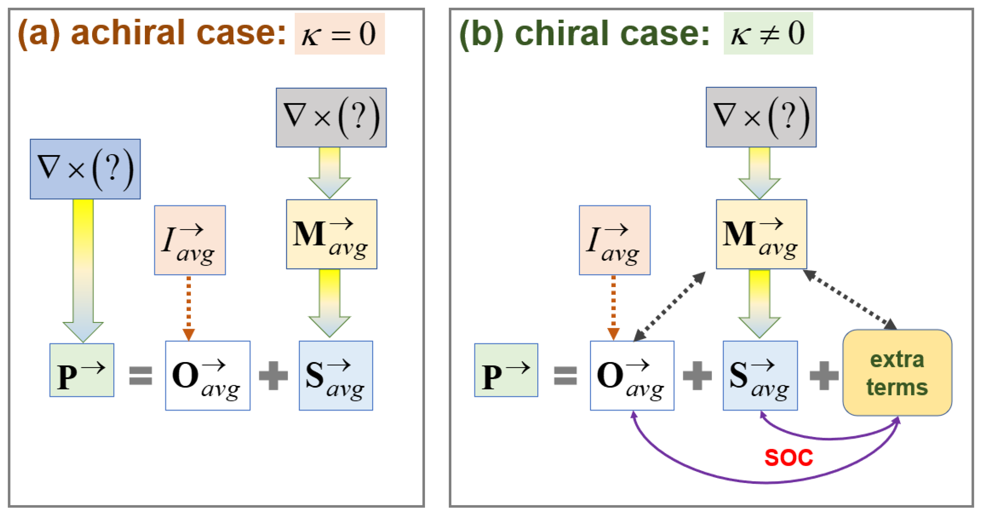
Based on the variables of the electric and magnetic fields of a certain EM wave, several key bilinear (‘quadratic’ inclusive) parameters can be formed for further analysis. Such a bilinear parameter can be formed either for an electric field or for a magnetic field. To be fair, an average parameter can be further constructed based on an electric–magnetic duality [12,13,14,15]. In this regard, the conventional, well-known parameters are here called active parameters. For instance, we recall an active field intensity, an active Poynting vector (or a linear momentum), an active spin linear momentum, an active orbital linear momentum, etc.

Of course, these active parameters are interrelated among them in a relatively straightforward manner for the EM waves through an achiral medium (often called here an ‘achiral case’). Notwithstanding, those interrelations become unbearably complicated for the EM waves propagating through a chiral medium (often called here a ‘chiral case’). A rough sketch of this distinction is presented in Figure 1.

A distinguishing feature of a chiral case is that the key bilinear parameters are interwoven by various forms of either spin–orbit coupling (SOC), spin–orbit conversion (SOC), or spin–orbit interaction (SOI) [10,16]. Figure 1b marks where SOCs might take place. The other aspect of the chiral case is that a well-organized hierarchy found for the achiral case is destroyed; namely, the key bilinear parameters are mixed up among them. This issue will be clarified later by comparing both Figure 1a,b.

Still, another aspect of the chiral case is that conservation laws become fuzzier because of the difficulty in finding suitable flux vectors that are operated on by the divergence operator $\nabla •$. In this regard, the question mark $\left(?\right)$ in Figure 1 signifies something that we could not find so far. In other words, the symbol $\nabla \times \left(?\right)$ with a downward arrow attached denotes a vector potential $\left(?\right)$, such that $\nabla •\left[\nabla \times \left(?\right)\right]=0$.

Figure 1a illustrates that an achiral medium gives rise to an orderly hierarchy, whereas Figure 1b depicts that a nonzero medium chirality renders key bilinear parameters interrelated among them. The presented key bilinear parameters include the energy density $I_{avg}^{\to }$, the Poynting vector $P^{\to }$, the linear momenta $\left\{O_{avg}^{\to },S_{avg}^{\to }\right\}$ (orbital and spin portions), and the spin angular momentum density $M_{avg}^{\to }$. These parameters are time-averaged ones for time-oscillatory fields in an unbounded space. In Figure 1b for a chiral medium, extra terms characterize spin–orbit couplings (SOCs), whereas there is a clear separation between $\left\{O_{avg}^{\to },S_{avg}^{\to }\right\}$ in Figure 1a for an achiral medium due to the absence of a SOC.

To each of these active bilinear parameters, we can associate a reactive bilinear parameter such as a reactive field intensity, a reactive Poynting vector, a reactive spin linear momentum, a reactive orbital linear momentum, etc. This set of reactive bilinear parameters has received less attention than the set of active bilinear parameters. See [15] for a recent review of reactive bilinear parameters from the viewpoint of conservation laws. There are other parameters that do not distinguish between active and reactive properties, for instance, the Stokes parameters. It is well-known that reactive bilinear parameters are more significant in the near field than in the far field [5,7]. In comparison, active bilinear parameters are dominant in the far field.

The basics of the conservation laws involving both active and reactive properties have been presented in our recent study [8] on the EM waves in chiral media. We have thus recognized several unconventional terms that arise from nonzero medium chirality while investigating obliquely propagating two-plane waves. Notwithstanding, we have missed in [8] properly recognizing the various interrelationships among those chirality-associated terms arising from nonzero medium chirality.

Therefore, this study focuses on the EM waves established in chiral dielectric media in a spatially unbounded domain. For simplicity, the chiral media are assumed to be loss-free so that the circular dichroism is not under consideration. Both active and reactive bilinear parameters are examined for their conservation laws while assuming temporally oscillatory EM fields. We will test the validity of our conservation laws with a plane wave of circular polarizations. In this way, we have identified in this study the implications of those extra chirality-associated terms in view of the interchange between the aforementioned spin and orbital linear momenta (viz., SOC). Such an SOC is known to take place across the interface between two different media if it ever took place [13]. In comparison, we discovered in this study that an SOC can take place in an unbounded chiral medium as well.

Our chiral case is one example of light–matter interactions. If a material’s response to illuminated light exhibits sign changes for certain parameters, we can then suspect that something similar to our medium chirality is involved, either in the constitutive relations of an average material or in the structure of constituent molecules. For instance, a material’s response could be different depending on the sign of the circular polarizations (clockwise versus counterclockwise) of the incident light. Such handedness-dependent responses often lead to diverse forms of Hall effects [10,16].

This paper is structured as follows. Section 2 presents the basic formulation. Section 3 handles the conservation laws focusing on a chiral case. Section 4 deals with the Poynting vector and the spin angular momentum for a chiral case, thus illustrating spin–orbit coupling. Section 5 summarizes the various formulas for the achiral case. Section 6 provides an example of a plane wave for the achiral case, thus pointing out several inconsistencies in the conservation laws for a chiral case. Section 7 considers what is necessary for well-posed electromagnetic problems. Section 8 offers discussions on various topics, including SOCs and quantum information. After a short epilogue in Section 9, Section 10 concludes our findings. We intended to make this paper self-contained; thus, we placed some details in Appendices.

2. Problem Formulation

The way of achieving dimensionless variables and parameters has already been presented in [8]. One exception is to make the temporal frequency explicit in this study [1]. We employ the overbar ¯ to denote the dimensional parameters and variables. Let $\left\{{\overline{\epsilon }}_0,{\overline{\mu }}_0\right\}$ be the dimensional electric permittivity and magnetic permeability in a vacuum. Furthermore, $\left\{{\overline{\omega }}_{ref},{\overline{t}}_{ref}\equiv 1/{\overline{\omega }}_{ref}\right\}$ are the reference frequency and the reference time. In addition, we define the reference magnitude ${\overline{E}}_{ref}$ for the electric field. We stress that only $\left\{{\overline{\omega }}_{ref},{\overline{E}}_{ref}\right\}$ are the arbitrary reference parameters at our disposal. Let us summarize the following set of reference parameters.

$$\begin{array}{l}{\overline{t}}_{ref}\equiv \frac{1}{{\overline{\omega }}_{ref}},{\overline{c}}_0\equiv \frac{1}{\sqrt{{\overline{\epsilon }}_0{\overline{\mu }}_0}},{\overline{Z}}_0\equiv \sqrt{\frac{{\overline{\mu }}_0}{{\overline{\epsilon }}_0}},{\overline{E}}_{ref},{\overline{H}}_{ref}=\frac{{\overline{E}}_{ref}}{{\overline{Z}}_0}\\ {\overline{L}}_{ref}\equiv {\overline{c}}_0{\overline{t}}_{ref}\equiv \frac{{\overline{c}}_0}{{\overline{\omega }}_{ref}}\equiv \frac{1}{{\overline{k}}_0},{\overline{k}}_0\equiv \frac{{\overline{\omega }}_{ref}}{{\overline{c}}_0}\end{array}.$$

(1)

Here, $\left\{{\overline{c}}_0,{\overline{Z}}_0\right\}$ are the light speed and impedance in a vacuum. In addition, $\left\{{\overline{L}}_{ref},{\overline{k}}_0\right\}$ are the reference length and reference wave number in a vacuum. Employing the above set of reference parameters in Equation (1), the relevant dimensionless parameters and variables are defined below.

$$\begin{array}{l}\omega \equiv \frac{\overline{\omega }}{{\overline{\omega }}_{ref}},t\equiv \frac{\overline{t}}{{\overline{t}}_{ref}},\nabla \equiv \frac{\overline{\nabla }}{{\overline{k}}_0},\epsilon \equiv \frac{\overline{\epsilon }}{{\overline{\epsilon }}_0},\mu \equiv \frac{\overline{\mu }}{{\overline{\mu }}_0}, ,\kappa \equiv {\overline{c}}_0\overline{\kappa }\\ E\equiv \frac{\overline{E}}{{\overline{E}}_{ref}},H\equiv \frac{\overline{H}}{{\overline{H}}_{ref}},D\equiv \frac{\overline{D}}{{\overline{\epsilon }}_0{\overline{E}}_{ref}},B\equiv \frac{{\overline{c}}_0\overline{B}}{{\overline{E}}_{ref}}\end{array}.$$

(2)

Therefore, the temporal oscillation factor $\exp \left(-i\overline{\omega }\overline{t}\right)$ for all of the field variables becomes $\exp \left(-i\omega t\right)$, after the dimensional frequency and time $\left\{\overline{\omega },\overline{t}\right\}$ become, respectively, the dimensionless ones $\left\{\omega ,t\right\}$. The spatial gradient is analogously made dimensionless from $\overline{\nabla }$ to $\nabla$. In addition, $\left\{\epsilon ,\mu \right\}$ are the dimensionless or relative electric permittivity and magnetic permeability, respectively. For the base dielectric, $\sqrt{\epsilon \mu }\equiv c_D^{-1}$ hence denotes a refractive index. The dimensional chirality parameter $\overline{\kappa }$ is made dimensionless to what is called a ‘chirality parameter’ $\kappa$.

The bold letters denote vectors. The dimensionless variables $\left\{E,H\right\}$ denote the electric and magnetic fields, respectively. Likewise, $\left\{D,B\right\}$ are dimensionless vectors for the electric displacement field and the magnetic induction field, respectively. Consequently, the Maxwell equations are cast into the following dimensionless forms.

$$\left\{\begin{array}{l}\nabla \times E=i\omega B\\ \nabla \times H=-i\omega D\end{array}\right.,\left\{\begin{array}{l}\nabla •D=0\\ \nabla •B=0\end{array}\right.,\left\{\begin{array}{l}D=\epsilon E+i\kappa H\\ B=\mu H-i\kappa E\end{array}\right..$$

(3)

Here, the first pair consists of the Faraday law $\nabla \times E=i\omega B$ and the Ampère law $\nabla \times H=-i\omega D$. The second pair consists of two divergence-free conditions. The third pair consists of constitutive relations [2,9,11]. By an achiral medium, we mean $\kappa =0$ in Equation (3), so that $\left\{D=\epsilon E,B=\mu H\right\}$ is obtained. We assume in this study a chiral dielectric to be loss-free, such that $\epsilon ,\mu >0$ and $\kappa \in ℝ$ so that a Pasteur medium is assumed.

Meanwhile, there is another pair of constitutive relations by the name of Drude–Born–Fedorov, which consists of $D=\epsilon \left(E+\beta \nabla \times E\right)$ and $B=\mu \left(H+\beta \nabla \times H\right)$ with $\beta$ being another kind of chirality parameter [2]. This pair of constitutive relations has been exclusively employed in [6] (pp. 181–194). Notwithstanding, our recent analysis of both types of constitutive relations in [8] confirms that both sets of constitutive relations lead to almost identical results when both $\left\{\kappa ,\beta \right\}$ are much smaller in magnitudes than unity. For this reason, we handle in this study only the constitutive relations provided in Equation (3).

The way the dimensionless governing equations are achieved in Equation (3) by use of the reference parameters listed in Equations (1) and (2) is almost identical to what was presented in [8]. In comparison to [8], the sole addition in Equation (3) is the dimensionless frequency $\omega$ such that the frequency effects can be explicitly accounted for throughout this study.

To solve the Maxwell equations in Equation (3), we introduce a pair $Q_{\pm }$ of circular vectors. The present pair of subscripts $\left\{+,-\right\}$ replaces the conventional pair of $\left\{L,R\right\}$, where a ‘left’ and a ‘right’ waves are, respectively, implied [3,6]. Let us introduce the following set of intermediaries.

$$\begin{array}{l}{c}_D\equiv \frac{1}{\sqrt{\epsilon \mu }},c_{\pm }\equiv \frac{1}{\sqrt{\epsilon \mu }\pm \kappa }\equiv \frac{c_D}{1\pm c_D\kappa },\epsilon \mu -{\kappa }^2\equiv \frac{1}{c_{+}{c}_{-}}\\ c_{avg}^{-+}\equiv \frac{1}{2}\left(c_{-}+c_{+}\right)=\frac{1}{c_D}\frac{1}{\epsilon \mu -{\kappa }^2}=\frac{c_{+}{c}_{-}}{c_D},{\Delta }_{-+}\equiv \frac{1}{2}\left(c_{-}-c_{+}\right)=\frac{\kappa }{\epsilon \mu -{\kappa }^2}\\ k_D\equiv \frac{\omega }{c_D}\equiv \omega \sqrt{\epsilon \mu },k_{\pm }\equiv \frac{\omega }{c_{\pm }}\equiv \omega \left(\sqrt{\epsilon \mu }\pm \kappa \right),\left\{\begin{array}{l}{c}_{\pm }>0\\ k_{\pm }>0\end{array}\right.\hspace{1em}\iff \hspace{1em}\left\{\begin{array}{l}\left|c_D\kappa \right|<1\\ \left|\kappa \right|<\sqrt{\epsilon \mu }\end{array}\right.\end{array}.$$

(4)

Here, the subscript ‘D’ signifies a base dielectric medium where chiral molecules might be homogeneously dispersed [2]. This pair $\left\{+,-\right\}$ of notations greatly facilitates our ensuing formulations.

It is well-established that the circular vectors $Q_{\pm }$ satisfy three conditions: (i) the divergence-free condition $\nabla •Q_{\pm }=0$, (ii) the curl condition $\nabla \times Q_{\pm }=\pm k_{\pm }{Q}_{\pm }$, and (iii) the Helmholtz equations ${\nabla }^2{Q}_{\pm }+k_{\pm }^2{Q}_{\pm }=0$. See [3] and the Supplementary Material of [8] for details. In this regard, it is often overlooked that $\left\{Q_{+},Q_{-}\right\}$ are in general neither parallel (co-polarized) nor perpendicular (cross-polarized) to each other [10,16]. In brief,

$$\nabla •Q_{\pm }=0,\nabla \times Q_{\pm }=\pm k_{\pm }{Q}_{\pm },{\nabla }^2{Q}_{\pm }+k_{\pm }^2{Q}_{\pm }=0.$$

(5)

We assume in this study that the chirality parameter is sufficiently small such that $c_{\pm }>0$ as stated in the last item of the third line of Equation (4). Therefore, both of $k_{\pm }$ are assumed positive even if $\kappa$ is allowed to take any sign.

Under such a boundedness property $\left|\kappa \right|<\sqrt{\epsilon \mu }$, $k_{\pm }>0$ implies from $\nabla \times Q_{\pm }=\pm k_{\pm }{Q}_{\pm }$ the physical circumstance that $\left\{Q_{+},Q_{-}\right\}$ are accompanied, respectively, by a positive vortex and a negative one. Such a pair of counter-rotating vortices is a hallmark of the EM waves prevailing through a chiral medium. Because of $k_{\pm }\equiv \omega \left(\sqrt{\epsilon \mu }\pm \kappa \right)$ in Equation (4), the vortex strength is linearly proportional to $\left|\kappa \right|$, while being directly proportional to $\omega$. Therefore, an optically denser medium with a larger refractive index of $\sqrt{\epsilon \mu }$ is associated with a larger vortex strength for a given $\omega$.

Once $Q_{\pm }$ are obtained, the EM fields are constructed by $E=Q_{+}-i{Z}_D{Q}_{-}$ and $H=-i{Z}_D^{-1}{Q}_{+}+Q_{-}$ [3,6]. Here, $Z_D\equiv \sqrt{\mu /\epsilon }$ is the impedance that represents the base dielectric as $c_D\equiv {\left(\epsilon \mu \right)}^{-1/2}$, defined in Equation (4). In summary,

$$Z_D\equiv \sqrt{\frac{\mu }{\epsilon }},\left\{\begin{array}{l}E=Q_{+}-i{Z}_D{Q}_{-}\\ H=-i{Z}_D^{-1}{Q}_{+}+Q_{-}\end{array}\right..$$

(6)

3. Conservation Laws for Chiral Cases

With the help of an arbitrary pair of once-differentiable vectors $A,B\in {ℂ}^3$, let us collect several vector identities that are essential to further developments.

$$\begin{array}{l}\left\{\begin{array}{l}\nabla •\left(A\times B\right)=\left(\nabla \times A\right)•B-\left(\nabla \times B\right)•A=B•\left(\nabla \times A\right)-A•\left(\nabla \times B\right)\\ A\times \left(\nabla \times B\right)=A•\left(\nabla \right)B-\left(A•\nabla \right)B\end{array}\right.\\ \nabla \times \left(A\times B\right)=\left(B•\nabla \right)A-\left(A•\nabla \right)B\begin{array}{c}\end{array}\Leftarrow \begin{array}{c}\end{array}\nabla •A=\nabla •B=0\\ A=\nabla \times B\begin{array}{c}\end{array}\iff \begin{array}{c}\end{array}\nabla •A=0\end{array}.$$

(7)

Both the first and the second vector identities do not demand the divergence-free constraints, whereas the third identity holds true under the additional constraints $\nabla •A=\nabla •B=0$. Let $\left\{x_i,{\widehat{e}}_i\right\}$ denote a generic pair of the Cartesian coordinate and its unit vector. By the Einstein summation notation for repeated indices, the convective derivative reads $\left(A•\nabla \right)B\equiv A_j\left(\partial B_i/\partial x_j\right){\widehat{e}}_i$, whereas the orbital derivative reads $A•\left(\nabla \right)B\equiv A_j\left(\partial B_j/\partial x_i\right){\widehat{e}}_i$. From physical perspectives, $\left(B•\nabla \right)A$ reads vector $A$ being transported or convected by $B$, whereas $\left(A•\nabla \right)B$ reads vector $B$ being transported by $A$.

In addition, the last identity of Equation (7) states that a solenoidal (divergence-free, incompressible) field $A$ is expressible as a vortex of a potential vector $B$. The converse also holds true as indicated by the double-head arrow ‘$\iff$’. This fundamental identity will be employed a couple of times in this study [2].

On the other hand, we can prove the following identity.

$$\mathrm{Re}\left[A^{\ast }•\left(\nabla \right)A\right]=\frac{1}{2}\mathrm{Re}\left(A_j^{\ast }\frac{\partial A_j}{\partial x_i}+A_j\frac{\partial A_j^{\ast }}{\partial x_j}\right){\widehat{e}}_i=\mathrm{Re}\left[\frac{1}{2}\frac{\partial \left(A_j^{\ast }{A}_j\right)}{\partial x_i}\right]{\widehat{e}}_i\equiv \nabla \left(\frac{1}{2}{\left|A\right|}^2\right).$$

(8)

Therefore, $\mathrm{Re}\left[A^{\ast }•\left(\nabla \right)A\right]=\nabla \left(\frac{1}{2}{A}^{\ast }•A\right)$ means that the orbital-like parameter is proportional to the spatial gradient of half the intensity. In contrast, $\mathrm{Im}\left[A^{\ast }•\left(\nabla \right)A\right]$ does not lend itself to such a neat formula. In fact, $\mathrm{Im}\left[A^{\ast }•\left(\nabla \right)A\right]$ is linked spins, as will be shortly discussed.

Let us introduce below the pair $\left\{I_{avg}^{\to },I_{avg}^{\Leftarrow }\right\}$ of the active and reactive energy densities together with the pair $\left\{M_{avg}^{\Rightarrow },M_{avg}^{\Leftarrow }\right\}$ of the active and reactive spin angular momentum (AM) densities [8,15].

$$\begin{array}{l}\left\{\begin{array}{l}{I}_E\equiv \epsilon E^{\ast }•E\\ I_H\equiv \mu H^{\ast }•H\end{array}\right.,\left\{\begin{array}{l}{M}_E^{\to }\equiv \epsilon \mathrm{Im}\left(E^{\ast }\times E\right)\\ M_H^{\to }\equiv \mu \mathrm{Im}\left(H^{\ast }\times H\right)\end{array}\right.\\ \left\{\begin{array}{l}{I}_{avg}^{\to }\equiv \frac{1}{2}\left(\epsilon E^{\ast }•E+\mu H^{\ast }•H\right)\\ J_{avg}^{\to }\equiv \frac{1}{2}\left(\epsilon E^{\ast }•E-\mu H^{\ast }•H\right)\end{array}\right.,\left\{\begin{array}{l}{M}_{avg}^{\to }\equiv \frac{1}{2}\mathrm{Im}\left(\epsilon E^{\ast }\times E+\mu H^{\ast }\times H\right)\\ M_{avg}^{\Leftarrow }\equiv \frac{1}{2}\mathrm{Re}\left(\epsilon E^{\ast }\times E+\mu H^{\ast }\times H\right)\end{array}\right.\end{array}.$$

(9)

Henceforth, we omit the factor of half that arises from time averaging. Operationally speaking, the cancellation $\exp \left(-i\omega t\right)\exp \left(i\omega t\right)=1$ applies to all bilinear (‘quadratic’ inclusive) parameters in Equation (9). In addition, these parameters are now real-valued since $\epsilon ,\mu >0$ are assumed for a base dielectric medium throughout this study. Resultantly, $I_{avg}^{\to }>0$. In addition, $\left\{I_{avg}^{\to },J_{avg}^{\to }\right\}$ are the active energy-sum (‘energy’, simply) density and the active energy-difference density, respectively. Both reactive energy densities $\left\{I_{avg}^{\Leftarrow },J_{avg}^{\Leftarrow }\right\}$ do not exist at all.

The subscripts $\left\{\to ,\Leftarrow \right\}$ in Equation (9) stand for ‘active’ and ‘reactive’, respectively. This pair $\left\{\to ,\Leftarrow \right\}$ is better readable than the symmetric pair $\left\{\Rightarrow ,\Leftarrow \right\}$, which we have worked with in [12]. Instead of ‘active’, we have employed ‘electromagnetic (EM)’ in our recent paper [8]. Ordinary readers might have been familiar with $\left\{I_{avg}^{\to },M_{avg}^{\to }\right\}$ in terms of conventional notation $\left\{I,M\right\}$, whereas $\left\{J_{avg}^{\to },M_{avg}^{\Leftarrow }\right\}$ are less discussed.

The subscripts $\left\{E,H\right\}$ in Equation (9) denote, respectively, the electric and magnetic portions, while the subscript ‘$avg$’ implies an average of the two. The three parameters $\left\{I_{avg}^{\to },M_{avg}^{\to },M_{avg}^{\Leftarrow }\right\}$ in Equation (9) are placed in the forms of the electric–magnetic duality [13,14]. In addition, most of the key bilinear parameters are expressed in terms of the modified pair $\left\{\sqrt{\epsilon }E,\sqrt{\mu }H\right\}$ instead of the pair $\left\{E,H\right\}$. Notice that $M_{avg}^{\to }$ signifies the states of polarization [5,10,12].

We further define the pair $\left\{P^{\to },P^{\Leftarrow }\right\}$ of the active and reactive Poynting vectors (also known as energy flow) and the pair $\left\{{\mathcal{C}}^{\to },{\mathcal{C}}^{\Leftarrow }\right\}$ of the active and reactive helicities [5,15].

$$\begin{array}{l}\left\{\begin{array}{l}{P}^{\to }\equiv {\omega }^{-1}\mathrm{Re}\left(E\times H^{\ast }\right)\\ P^{\Leftarrow }\equiv {\omega }^{-1}\mathrm{Im}\left(E\times H^{\ast }\right)\end{array}\right.,\left\{\begin{array}{l}{\mathcal{C}}^{\to }\equiv \mathrm{Im}\left(E•H^{\ast }\right)\\ {\mathcal{C}}^{\Leftarrow }\equiv \mathrm{Re}\left(E•H^{\ast }\right)\end{array}\right.\\ \left\{\begin{array}{l}{P}_{avg}^{\to }\equiv P^{\to }\\ P_{avg}^{\Leftarrow }\equiv P^{\Leftarrow }\end{array}\right.,\left\{\begin{array}{l}{\mathcal{C}}_{avg}^{\to }\equiv {\mathcal{C}}^{\to }\\ {\mathcal{C}}_{avg}^{\Leftarrow }\equiv {\mathcal{C}}^{\Leftarrow }\end{array}\right.\end{array}.$$

(10)

Instead of $P^{\to }\equiv \mathrm{Re}\left(E\times H^{\ast }\right)$, as previously defined in [8], we now have an explicit frequency dependence by $P^{\to }\equiv {\omega }^{-1}\mathrm{Re}\left(E\times H^{\ast }\right)$ in conformance to the formulas in [14]. Both pairs $\left\{P^{\to },P^{\Leftarrow }\right\}$ and $\left\{{\mathcal{C}}^{\to },{\mathcal{C}}^{\Leftarrow }\right\}$ are already placed in the electric–magnetic dual forms. Consequently, we have $\left\{P_{avg}^{\to },P_{avg}^{\Leftarrow }\right\}\equiv \left\{P^{\to },P^{\Leftarrow }\right\}$ and $\left\{{\mathcal{C}}_{avg}^{\to },{\mathcal{C}}_{avg}^{\Leftarrow }\right\}\equiv \left\{{\mathcal{C}}^{\to },{\mathcal{C}}^{\Leftarrow }\right\}$.

Notice in Equation (9) that $\left\{I_{avg}^{\to },J_{avg}^{\to }\right\}$ are complementary in one sense that $I_{avg}^{\to }+J_{avg}^{\to }=\epsilon E^{\ast }•E$ and $I_{avg}^{\to }-J_{avg}^{\to }=\mu H^{\ast }•H$. In comparison, we define below the complex parameters $\left\{M_{avg}^{ℂ},P^{ℂ},{\mathcal{C}}^{ℂ}\right\}$ based on Equations (9) and (10),

$$\begin{array}{l}{I}_{avg}^{ℂ}\equiv I_{avg}^{\to }+i{J}_{avg}^{\to }\\ M_{avg}^{ℂ}\equiv M_{avg}^{\Leftarrow }+i{M}_{avg}^{\to },\begin{array}{c}\end{array}{P}^{ℂ}\equiv P^{\to }+i{P}^{\Leftarrow },\begin{array}{c}\end{array}{\mathcal{C}}^{ℂ}\equiv {\mathcal{C}}^{\Leftarrow }+i{\mathcal{C}}^{\to }\end{array}.$$

(11)

We thus learn that the pair $\left\{\to ,\Leftarrow \right\}$ implies the real and imaginary parts (or vice versa) of a pertinent complex property.

Let us form the dot products $\left(\nabla \times E=i\omega B\right)•H^{\ast }$ and $\left(\nabla \times H=-i\omega D\right)•E^{\ast }$, respectively, for the Faraday and Ampère laws in Equation (3). Taking the difference and the sum of the resulting two relations, we obtain the following pair of energy conservation laws [8].

$$\begin{array}{l}\left\{\begin{array}{l}{I}_{avg}^{\to }+i\nabla •P_{avg}^{\to }+i\frac{1}{2}{g}_{+}=-\kappa {\mathcal{C}}_{avg}^{\to }\\ J_{avg}^{\to }+\nabla •P_{avg}^{\Leftarrow }-i\frac{1}{2}{g}_{-}=-i\kappa {\mathcal{C}}_{avg}^{\Leftarrow }\end{array}\right.\hspace{1em}\Rightarrow \\ I_{avg}^{ℂ}+i\nabla •P^{ℂ}+i\frac{1}{2}\left(g_{+}+i{g}_{-}\right)=-\kappa \left({\mathcal{C}}_{avg}^{\to }+{\mathcal{C}}_{avg}^{\Leftarrow }\right)\\ g_{\pm }\equiv \frac{1}{\omega }\left[E•\left(\nabla \times H^{\ast }\right)\mp H•{\left(\nabla \times E\right)}^{\ast }\right]\end{array}.$$

(12)

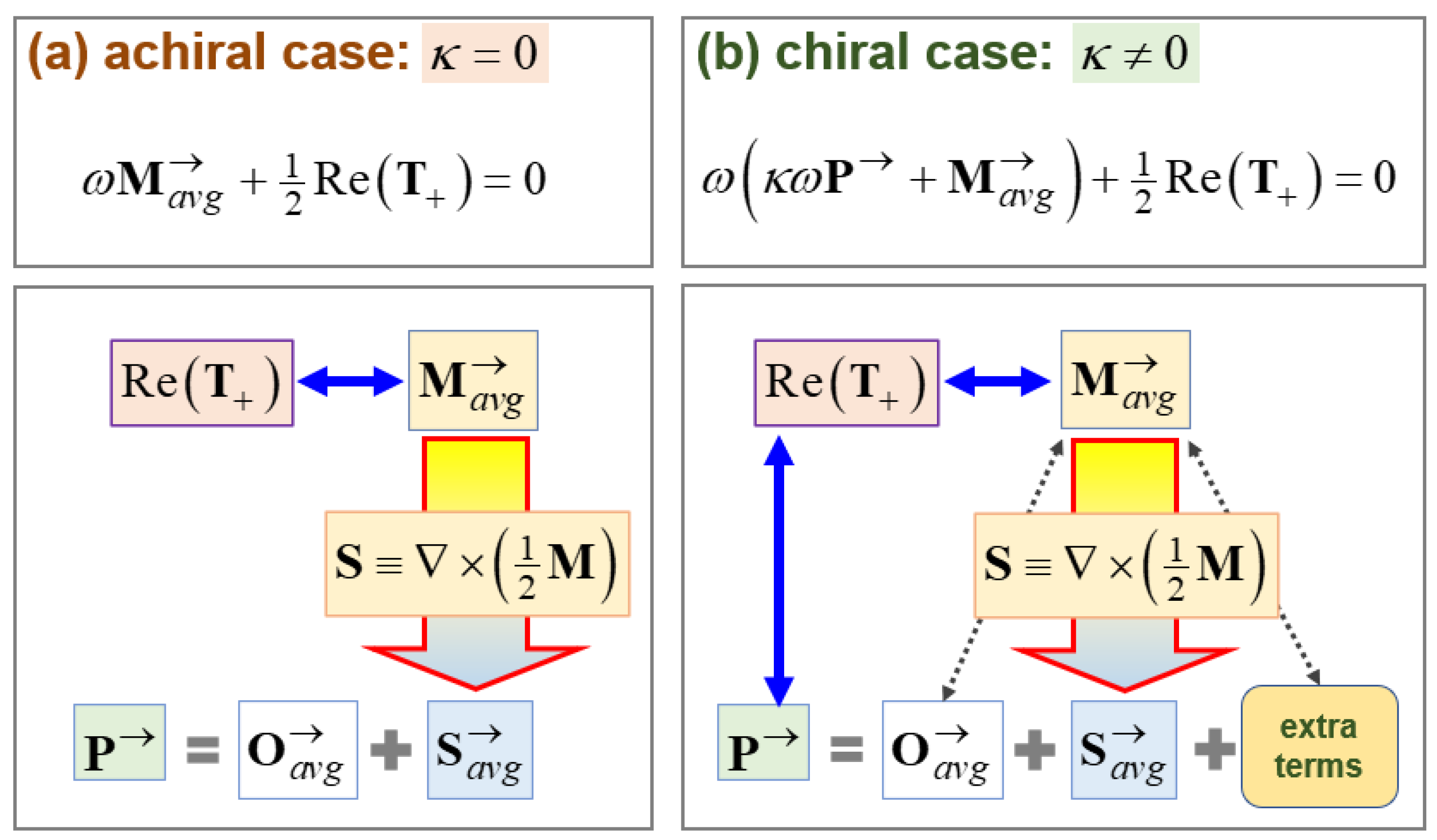
Here, we have utilized the suitable vector identities in Equation (7). In the last line of Equation (12), we encounter another complex parameter $g_{+}+i{g}_{-}$, while the combined helicity ${\mathcal{C}}_{avg}^{\to }+{\mathcal{C}}_{avg}^{\Leftarrow }$ fits neither the expected complex helicity ${\mathcal{C}}_{avg}^{\to }+i{\mathcal{C}}_{avg}^{\Leftarrow }$ nor ${\mathcal{C}}^{ℂ}\equiv {\mathcal{C}}^{\Leftarrow }+i{\mathcal{C}}^{\to }$ in Equation (11).

Reactive properties are discussed in detail by [12,15]. We could find ample applications in connection, especially with antenna theory [5,8,12]. These reactive properties play significant roles, normally in the near field of a certain nanostructure immersed in either an achiral or chiral medium. Mathematically speaking, a certain active property and its reactive property make a pair of complex conjugates so that their analytical handling becomes easier than dealing only with an active property, as seen in Equations (11) and (12). In addition, much deeper issues lie in the Lagrangian formulations of dynamical systems.

We can easily separate the two leading lines of Equation (12) into the following two pairs after some shuffling [15].

$$\left\{\begin{array}{l}\frac{1}{2}\mathrm{Re}\left(g_{+}\right)+\nabla •P^{\to }=0\\ J_{avg}^{\to }+\frac{1}{2}\mathrm{Im}\left(g_{-}\right)+\nabla •P^{\Leftarrow }=0\end{array}\right.,\left\{\begin{array}{l}{I}_{avg}^{\to }+\kappa {\mathcal{C}}^{\to }=\frac{1}{2}\mathrm{Im}\left(g_{+}\right)\\ \frac{1}{2}\mathrm{Re}\left(g_{-}\right)=\kappa {\mathcal{C}}^{\Leftarrow }\end{array}\right..$$

(13)

The most distinguishing feature in this set of conservation laws obtained for a chiral medium is the interactions among the two active energy densities $\left\{I_{avg}^{\to },J_{avg}^{\to }\right\}$, the Poynting vectors $\left\{P^{\to },P^{\Leftarrow }\right\}$, and the helicities $\left\{{\mathcal{C}}^{\to },{\mathcal{C}}^{\Leftarrow }\right\}$ [15]. In addition, Equation (13) shows that the two members $\left\{\kappa {\mathcal{C}}_{avg}^{\to },\kappa {\mathcal{C}}_{avg}^{\Leftarrow }\right\}$ carry the respective multiplier $\kappa$, which means, in turn, that $\left\{{\mathcal{C}}_{avg}^{\to },{\mathcal{C}}_{avg}^{\Leftarrow }\right\}$ are, respectively, odd in $\kappa$. This is the reason why both (active and reactive) helicities $\left\{{\mathcal{C}}_{avg}^{\to },{\mathcal{C}}_{avg}^{\Leftarrow }\right\}$ are sometimes called the (active and reactive) field chirality parameters [8].

4. Spins and Breakdown of Energy Flows

With both electric and magnetic portions $\left\{M_E^{\to },M_H^{\to }\right\}$ defined in Equation (9), let us take the divergence of the spin AM $M_{avg}^{\to }\equiv \frac{1}{2}\left(M_E^{\to }+M_H^{\to }\right)$.

$$\left\{\begin{array}{l}\nabla •M_E^{\to }=-2\omega \epsilon \mu {\mathcal{C}}^{\Leftarrow }\\ \nabla •M_H^{\to }=2\omega \epsilon \mu {\mathcal{C}}^{\Leftarrow }\end{array}\right.\hspace{1em}\Rightarrow \hspace{1em}\nabla •M_{avg}^{\to }=0.$$

(14)

Here, we have made use of the Maxwell equations in Equation (3) along with the vector identities in Equation (7). See Appendix A for the derivation of Equation (14). From a physical point of view, $\nabla •M_{avg}^{\to }=0$ signifies the conservation of $M_{avg}^{\to }$, for which we could find its potential according to the last vector identity in Equation (7). The self-cancelling feature $\nabla •M_{avg}^{\to }=0$ between $\left\{\nabla •M_E^{\to },\nabla •M_H^{\to }\right\}$ has been fully discussed with a proper example, with the EM fields induced by electric point dipoles [12]. Notice hence that Equation (14) holds true not only to an achiral case but also to a chiral case. This fact $\nabla •M_{avg}^{\to }=0$ means that we need to examine $\left\{\nabla •M_E^{\to },\nabla •M_H^{\to }\right\}$ separately for a chiral case.

Setting $A=B^{\ast }$ in the first vector identity of Equation (7) and taking the imaginary parts leads to $\mathrm{Im}\left[\nabla \times \frac{1}{2}\left(B^{\ast }\times B\right)\right]=-\mathrm{Im}\left[\left(B^{\ast }•\nabla \right)B\right]$. This vector identity is then applied to form the curl $\nabla \times M_{avg}^{\to }$ of the average spin AM $M_{avg}^{\to }\equiv \frac{1}{2}\left(M_E^{\to }+M_H^{\to }\right)$ in the following manner by consulting $\left\{M_E^{\to },M_H^{\to }\right\}$, as defined in Equation (9).

$$\begin{array}{l}\left\{\begin{array}{l}\nabla \times \left(\frac{1}{2}{M}_E^{\to }\right)=-\epsilon \mathrm{Im}\left[\left(E^{\ast }•\nabla \right)E\right]\equiv S_E^{\to }\\ \nabla \times \left(\frac{1}{2}{M}_H^{\to }\right)=-\mu \mathrm{Im}\left[\left(H^{\ast }•\nabla \right)H\right]\equiv S_H^{\to }\end{array}\right.,\left\{\begin{array}{l}{S}_E^{\Leftarrow }\equiv -\epsilon \mathrm{Im}\left[\left(E^{\ast }•\nabla \right)E\right]\\ S_H^{\Leftarrow }\equiv -\mu \mathrm{Im}\left[\left(H^{\ast }•\nabla \right)H\right]\end{array}\right.\hspace{1em}\Rightarrow \\ \left\{\begin{array}{l}{S}_{avg}^{\to }\equiv -\frac{1}{2}\mathrm{Im}\left[\epsilon \left(E^{\ast }•\nabla \right)E+\mu \left(H^{\ast }•\nabla \right)H\right]\equiv \nabla \times \left(\frac{1}{2}{M}_{avg}^{\to }\right)\\ S_{avg}^{\Leftarrow }\equiv -\frac{1}{2}\mathrm{Re}\left[\epsilon \left(E^{\ast }•\nabla \right)E+\mu \left(H^{\ast }•\nabla \right)H\right]\end{array}\right.\end{array}.$$

(15)

In this way, the average spin linear momentum $S_{avg}^{\to }$ is defined as half the curl of $M_{avg}$. The idea behind this definition $\nabla \times \left(\frac{1}{2}{M}_{avg}^{\to }\right)=S_{avg}^{\to }$ is that $S_{avg}^{\to }$ is divergence-free, namely, $\nabla •S_{avg}^{\to }=0$. In other words, $\frac{1}{2}{M}_{avg}^{\to }$ serves as a vector potential for $S_{avg}^{\to }$.

As a counterpart of $\left\{S_{avg}^{\to },S_{avg}^{\Leftarrow }\right\}$, the average orbital linear momenta $\left\{O_{avg}^{\to },O_{avg}^{\Leftarrow }\right\}$ are defined below.

$$\begin{array}{l}\left\{\begin{array}{l}{O}_E^{\to }\equiv \epsilon \mathrm{Im}\left[E^{\ast }•\left(\nabla \right)E\right]\\ O_H^{\to }\equiv \mu \mathrm{Im}\left[H^{\ast }•\left(\nabla \right)H\right]\end{array}\right.,\left\{\begin{array}{l}{O}_E^{\Leftarrow }\equiv \epsilon \mathrm{Re}\left[E^{\ast }•\left(\nabla \right)E\right]\\ O_H^{\Leftarrow }\equiv \mu \mathrm{Re}\left[H^{\ast }•\left(\nabla \right)H\right]\end{array}\right.\hspace{1em}\Rightarrow \\ \left\{\begin{array}{l}{O}_{avg}^{\to }\equiv \frac{1}{2}\mathrm{Im}\left[\epsilon E^{\ast }•\left(\nabla \right)E+\mu H^{\ast }•\left(\nabla \right)H\right]\\ O_{avg}^{\Leftarrow }\equiv \frac{1}{2}\mathrm{Re}\left[\epsilon E^{\ast }•\left(\nabla \right)E+\mu H^{\ast }•\left(\nabla \right)H\right]\end{array}\right.\end{array}.$$

(16)

Therefore, we can exploit Equation (8) in defining the following pair of average reactive orbital linear momenta $\left\{O_{avg}^{\Leftarrow },V_{avg}^{\Leftarrow }\right\}$.

$$\left\{\begin{array}{l}{O}_{avg}^{\Leftarrow }\equiv \frac{1}{2}\mathrm{Re}\left[\epsilon E^{\ast }•\left(\nabla \right)E+\mu H^{\ast }•\left(\nabla \right)H\right]=\frac{1}{2}\nabla \left(\frac{1}{2}\epsilon {\left|E\right|}^2+\frac{1}{2}\mu {\left|H\right|}^2\right)\equiv \frac{1}{2}\nabla I_{avg}^{\to }\\ V_{avg}^{\Leftarrow }\equiv \frac{1}{2}\mathrm{Re}\left[\epsilon E^{\ast }•\left(\nabla \right)E-\mu H^{\ast }•\left(\nabla \right)H\right]=\frac{1}{2}\nabla \left(\frac{1}{2}\epsilon {\left|E\right|}^2-\frac{1}{2}\mu {\left|H\right|}^2\right)\equiv \frac{1}{2}\nabla J_{avg}^{\to }\end{array}\right..$$

(17)

In this way, we invert the constitutive relations in Equation (3) to express $\left\{E,H\right\}$ in terms of their curls $\left\{\nabla \times E,\nabla \times H\right\}$ in the following fashion.

$$\left\{\begin{array}{c}E\\ H\end{array}\right\}=\frac{1}{\omega }\frac{i}{\epsilon \mu -{\kappa }^2}\left(\begin{array}{cc}i\kappa & \mu \\ -\epsilon & i\kappa \end{array}\right)\left\{\begin{array}{c}\nabla \times E\\ \nabla \times H\end{array}\right\}.$$

(18)

Furthermore, we introduce the following pair of intermediaries.

$$T_{\pm }\equiv H^{\ast }•\left(\nabla \right)E-\left(H^{\ast }•\nabla \right)E\pm \left[\left(E^{\ast }•\nabla \right)H-E^{\ast }•\left(\nabla \right)H\right].$$

(19)

Recall the complex Poynting vector $P^{ℂ}\equiv P^{\to }+i{P}^{\Leftarrow }\equiv {\omega }^{-1}E\times H^{\ast }$ defined previously in Equation (11).

Because both $\left\{E,H\right\}$ show up in $P^{ℂ}$, there are two ways of treating $P^{\to }$ by use of Equation (18). One way is to replace $H$ with its pair of curls in $P^{\to }\equiv {\omega }^{-1}\mathrm{Re}\left(E\times H^{\ast }\right)$, whereas the other way is to replace $E$ with its pair of curls in $P^{\to }\equiv {\omega }^{-1}\mathrm{Re}\left(E\times H^{\ast }\right)$. We then take the real and imaginary parts of $P^{ℂ}$ to find both $\left\{P^{\to },P^{\Leftarrow }\right\}$ as follows.

$$\left\{\begin{array}{l}{\omega }^2{P}^{\to }=c_{+}{c}_{-}\left(O_{avg}^{\to }+S_{avg}^{\to }\right)+\frac{1}{2}{\Delta }_{-+}\mathrm{Re}\left(T_{+}\right)\\ {\omega }^2{P}^{\Leftarrow }=c_{+}{c}_{-}\left(O_{avg}^{\to }+S_{avg}^{\to }\right)+\frac{1}{2}{\Delta }_{-+}\mathrm{Im}\left(T_{-}\right)\end{array}\right..$$

(20)

Here, we made use of Equations (16), (17), and (19). In addition, $\left\{c_{+},c_{-}\right\}$ and the mean speed difference ${\Delta }_{-+}$ were defined before in Equation (4) [1]. This finding in Equation (20) makes a key contribution to this study. It is noteworthy that our SOCs take place inside a single uniform chiral medium. The two terms $\left\{\frac{1}{2}{\Delta }_{-+}\mathrm{Re}\left(T_{+}\right),\frac{1}{2}{\Delta }_{-+}\mathrm{Im}\left(T_{-}\right)\right\}$ in Equation (20) signify the spin–orbit couplings (SOCs) (or conversions), respectively, in the active and reactive EM fields. In comparison, an SOC taking place across an interface between two dissimilar media is discussed in [13].

Consider next the active spin AM density $M_{avg}^{\to }$ by averaging its constituents $\left\{M_E^{\to },M_H^{\to }\right\}$ defined in Equation (9) while by expressing $\left\{E,H\right\}$ in terms of their curls $\left\{\nabla \times E,\nabla \times H\right\}$ according to Equation (18). Resultantly, we obtain the following set.

$$\begin{array}{l}\omega M_{avg}^{\to }=-{\Delta }_{-+}\left(O_{avg}^{\to }+S_{avg}^{\to }\right)-\frac{c_{+}{c}_{-}}{c_D^2}\frac{1}{2}\mathrm{Re}\left(T_{+}\right)\hspace{1em}\Rightarrow \\ \omega M_{avg}^{\to }=-{\Delta }_{-+}\left[O_{avg}^{\to }+\nabla \times \left(\frac{1}{2}{M}_{avg}^{\to }\right)\right]-\frac{c_{+}{c}_{-}}{c_D^2}\frac{1}{2}\mathrm{Re}\left(T_{+}\right)\end{array}.$$

(21)

Consequently, a medium chirality gives rise to another kind of SOC, which is the term $c_D^{-2}{c}_{+}{c}_{-}\frac{1}{2}\mathrm{Re}\left(T_{+}\right)$ in Equation (21).

Meanwhile, we have shown in Equation (15) that $S_{avg}^{\to }=\nabla \times \left(\frac{1}{2}{M}_{avg}^{\to }\right)$ holds true regardless of the medium chirality. We can think of the relation $S_{avg}^{\to }=\nabla \times \left(\frac{1}{2}{M}_{avg}^{\to }\right)$ as sort of a hierarchy since $S_{avg}^{\to }$ serving as a child (a derivative) is a spatial derivative of $M_{avg}^{\to }$ serving as a parent (an integral or a potential). The second relation in Equation (21) indicates essentially a recursive relation in $M_{avg}^{\to }$ since $M_{avg}^{\to }$ appears both as a child and as a parent. Such a mixed or confused hierarchy has already appeared in Equation (20). The last relation of Equation (21) tells that the member of the triplet $\left\{M_{avg}^{\to },O_{avg}^{\to },S_{avg}^{\to }\right\}$ now occupy the same hierarchy or level. This hierarchy issue has been discussed in our recent paper [12] for an achiral medium. We have thus extended this hierarchy structure to the chiral case in this study, thereby constituting another key contribution to it.

5. Reduction to the Achiral Case

It is helpful to separately consider an achiral case by setting $\kappa =0$ in all of the formulas presented so far. Let us now evaluate $g_{\pm }$ in Equation (12) for an achiral medium, for which $\nabla \times E=i\omega \mu H$ and $\nabla \times H=-i\omega \epsilon E$. Resultantly, we obtain $\left\{g_{+},g_{-}\right\}=2i\left\{I_{avg}^{\to },J_{avg}^{\to }\right\}$ for $\kappa =0$. Accordingly, Equation (13) is reduced to the following simpler set.

$$\kappa =0:\hspace{1em}\left\{\begin{array}{l}\nabla •P^{\to }=0\\ 2J_{avg}^{\to }+\nabla •P^{\Leftarrow }=0\end{array}\right.,\left\{\begin{array}{l}{I}_{avg}^{\to }=I_{avg}^{\to }\\ 0=0\end{array}\right..$$

(22)

In the first pair of Equation (22), $\nabla •P^{\to }=0$ is the familiar energy conservation law. In comparison, $2J_{avg}^{\to }+\nabla •P^{\Leftarrow }=0$ has been explicitly derived in [8] for the first time, although its variants have been presented elsewhere [15]. Meanwhile, the second pair of Equation (22) is trivially satisfied. The extra terms in Equation (13) in comparison to Equation (22) also been identified by [2].

Conservations laws for time-oscillatory field variables can be symbolically put into a generic form $\left(\oplus \right)+\nabla •\left(\otimes \right)=0$ for time-oscillatory fields. Here, the leaning term $\left(\oplus \right)$ refers to something to be conserved, whereas the second term $\nabla •\left(\otimes \right)$ means the spatial divergence of a flux $\left(\otimes \right)$. As an example, the relation $\nabla •P^{\to }=0$ in Equation (22) is an extreme case where $\left(\oplus \right)=0$. On the other hand, the other relation $2J_{avg}^{\to }+\nabla •P^{\Leftarrow }=0$ in Equation (22) fits perfectly into $\left(\oplus \right)+\nabla •\left(\otimes \right)=0$. This is another reason why the pair $\left\{2J_{avg}^{\to },P^{\Leftarrow }\right\}$ of the active energy-difference density and the reactive Poynting vector is endowed with a legitimate physical importance [15].

Consider Equation (13) for a chiral medium with $\kappa \ne 0$. The two relations $\frac{1}{2}\mathrm{Re}\left(A_{+}\right)+\nabla •P=0$ and $J_{avg}^{\to }+\frac{1}{2}\mathrm{Im}\left(g_{-}\right)+\nabla •R=0$ in Equation (13) still fit into the generic form $\left(\oplus \right)+\nabla •\left(\otimes \right)=0$. In comparison, the two relations $I_{avg}^{\to }=\frac{1}{2}\mathrm{Im}\left(g_{+}\right)-\kappa {\mathcal{C}}^{\to }$ and $\frac{1}{2}\mathrm{Re}\left(g_{-}\right)=\kappa \mathcal{K}$ in the second pair of Equation (13) do not fit into $\left(\oplus \right)+\nabla •\left(\otimes \right)=0$. Instead, these two relations offer couplings between the conserved parameters in the first pair of Equation (13) to the two helicity parameters $\left\{{\mathcal{C}}^{\to },{\mathcal{C}}^{\Leftarrow }\right\}$.

It is well-known for an achiral medium that the active helicity ${\mathcal{C}}^{\to }$ serves as the conserved parameter $\left(\oplus \right)$, whereas the average spin angular momentum (AM) density $M_{avg}^{\to }$ defined in Equation (9) served as the flux $\left(\otimes \right)$ [15]. In other words, the pair $\left\{{\mathcal{C}}^{\to },M_{avg}^{\to }\right\}$ constitutes what is called the ‘chirality (or helicity) conservation law’. The four relations in Equation (13) obtained for a chiral medium show complicated interrelationships among the set of various participating bilinear parameters $\left\{I_{avg}^{\to },J_{avg}^{\to },P^{\to },P^{\Leftarrow },{\mathcal{C}}^{\to },{\mathcal{C}}^{\Leftarrow },g_{\pm }\right\}$. This delicate picture leads us to looking into the spin AM $M_{avg}$ in depth.

It is useful to examine Equation (20) for an achiral medium with $\kappa =0$.

$$\kappa =0:\hspace{1em}\left\{\begin{array}{l}{\omega }^2\epsilon \mu P^{\to }\equiv k_D^2{P}^{\to }=O_{avg}^{\to }+S_{avg}^{\to }\\ {\omega }^2\epsilon \mu P^{\Leftarrow }\equiv k_D^2{P}^{\Leftarrow }=O_{avg}^{\Leftarrow }+S_{avg}^{\Leftarrow }\end{array}\right..$$

(23)

Therefore, both active and reactive Poynting vectors are completely separable into their respective spin and orbital portions. Such an achiral case has already been investigated for the free-space EM fields induced by electric point dipoles in [12]. Meanwhile, Equation (21) is reduced to $\omega M_{avg}^{\to }=-c_D^{-2}{c}_{+}{c}_{-}\frac{1}{2}\mathrm{Re}\left(T_{+}\right)$ for the achiral medium with $c_{+}{c}_{-}\propto \kappa =0$, thereby being not linked to $O_{avg}^{\to }+S_{avg}^{\to }$ in connection with Equation (23).

When comparing the reduced formulas presented in this section for the achiral case to those presented in both Section 3 and Section 4 for the chiral case, the additional terms arising from the medium chirality are linked to SOCs. This mixed-up situation for the chiral case is illustrated in Figure 1b in comparison to a relatively neat situation for the achiral case illustrated in Figure 1a.

We have already examined in [7,12] several features of both active and reactive bilinear parameters for the achiral cases. However, these two problems simultaneously share common features and distinctive differences. In [12], the EM fields induced by an electric point dipole are investigated mostly using analytical ways. Many of those analytical formulas indeed show that the reactive bilinear parameters are non-negligible only in the near field (not far field) of a singularity (i.e., an EM source) immersed in an achiral medium. Consequently, there are no SOCs in this dipole-induced EM field. In general, the reactive bilinear parameters play a greater role than active bilinear parameters in assessing light–matter interactions that are necessary for the proper designs of nano-antennas or optical nano-probes [4,5,12].

Meanwhile, we have examined in [7] the EM fields scattered off a dielectric (achiral) sphere that is immersed in another dielectric embedding medium. This Mie scattering problem is a standard subject handled in textbooks, such as [6]. We have examined in [7] its near-field behaviors, which have seldom been considered. Our findings in [7] show not only the importance of the reactive bilinear parameters but also the existence of SOCs.

How could such an achiral case in [7] exhibit SOCs, unlike the achiral case considered in [12]? The answer to this all-dielectric system in [7] for the Mie scattering lies in the existence of the interference effects arising from the interaction between the incident plane wave (this alone being examined in the next section) and the scattered field. From another perspective, we find both a transverse-magnetic (TM) mode and a transverse-electric (TE) mode in the solution to the Mie scattering. In other words, all six components of $\left\{E,H\right\}$ are nonzero generically for the Mie scatterings [6]. The Mie scattering off a dielectric sphere immersed in a chiral media considered by [3] belongs to a genuine chiral case according to the classification of this study. Therefore, we find in [3] not only the coexistence of both TM and TE modes but also nonzero SOCs. Resultantly, the Mie scatterings provide a possibility of magneto–electric coupling [15].

6. Example by a Plane Wave

For the achiral case with $\kappa =0$, consider a plane wave of a linear polarization being denoted by the subscript ‘$lin$’.

$$k_D\equiv \frac{\omega }{c_D}\equiv \omega \sqrt{\epsilon \mu },{\Pi }_D\equiv \exp \left(i{k}_{D}z\right),\left\{\begin{array}{l}{E}_{lin}=Q_{lin}\widehat{x}{\Pi }_D\\ i{Z}_D{H}_{lin}=Q_{lin}i\widehat{y}{\Pi }_D\end{array}\right..$$

(24)

Here, $\left\{x,y,z\right\}$ and $\left\{\widehat{x},\widehat{y},\widehat{z}\right\}$ denote the Cartesian coordinates and the corresponding unit vectors. Recall from Equation (4) that $k_D\equiv \omega /c_D\equiv \omega \sqrt{\epsilon \mu }$, which represents the base dielectric with $\kappa =0$. Although the magnetic field is given by $H_{lin}=Z_D^{-1}{Q}_D\widehat{y}{\Pi }_D$, it is written as $i{Z}_D{H}_{lin}=Q_{lin}i\widehat{y}{\Pi }_D$ in Equation (24) for easier comparison with others in the following. The complex magnitude parameter $Q_{lin}$ is completely at our disposal.

Along the same line of reasoning, consider a single plane wave of circular polarization being denoted by the subscript ‘$cir$’. For instance, one of its solutions is given by the following.

$$\left\{\begin{array}{l}\sqrt{2}{E}_{cir}=Q_{cir}\left(\widehat{x}+i\widehat{y}\right){\Pi }_D\\ \sqrt{2}i{Z}_D{H}_{cir}=Q_{cir}\left(\widehat{x}+i\widehat{y}\right){\Pi }_D\end{array}\right..$$

(25)

Once again, we are left with the single complex magnitude parameter of $Q_{cir}$ as the sole undetermined coefficient.

Both solutions in Equations (24) and (25) should satisfy the Faraday law $\nabla \times E=i\omega \mu H$ and the Ampère law $\nabla \times H=-i\omega \epsilon E$ reduced from Equation (3) for $\kappa =0$. Although we have conducted such proofs, they are not presented here for simplicity. Meanwhile, both divergence-free conditions $\nabla •E=\nabla •H=0$ are almost trivial to prove. Likewise, both Helmholtz equations ${\nabla }^{2}E+k_D^{2}E={\nabla }^{2}H+k_D^{2}H=0$ are satisfied by looking into the phase factor ${\Pi }_D\equiv \exp \left(i{k}_{D}z\right)$ that is common to both Equations (24) and (25).

From physical perspectives, the comparison of the solutions presented in Equations (24) and (25) is rewarding. Firstly, the fields $\left\{E_{lin},H_{lin}\right\}$ from Equation (24) are perpendicular to each other, while the fields $\left\{E_{cir},H_{cir}\right\}$ from Equation (25) are parallel to each other. Secondly, the fields $\left\{E_{lin},H_{lin}\right\}$ are in-phase with each other, while the fields $\left\{E_{cir},H_{cir}\right\}$ are out-of-phase (or in quadrature) to each other. Thirdly, both $\left\{E_{lin},H_{lin}\right\}$ and $\left\{E_{cir},H_{cir}\right\}$ are transverse to the wave-propagation $z$-direction. Fourthly, both $\left\{E_{lin},H_{lin}\right\}$ and $\left\{E_{cir},H_{cir}\right\}$ admit a single specifiable complex magnitude, namely, $Q_{lin}$ or $Q_{cir}$.

With the above backgrounds obtained for the achiral case, we turn now to the chiral case with $\kappa \ne 0$. Consider a plane wave of circular polarization inherent in the representation by the circular vector $Q_{\pm }$, as follows [2,3,6].

$$Q_{\pm }=Q_{\pm }\frac{1}{\sqrt{2}}\left(\widehat{x}\pm i\widehat{y}\right)\exp \left(i{k}_{\pm }z\right).$$

(26)

In addition, the two distinct parameters $\left\{Q_{+},Q_{-}\right\}$ are complex scalars, i.e., $Q_{\pm }\in ℂ$. Unlike Equation (24), it is stressed that no linearly polarized EM fields are meaningful for this chiral case. The circular vectors in Equation (26) satisfy all three constraints presented in Equation (5). Especially, the curl condition $\nabla \times Q_{\pm }=\pm k_{\pm }{Q}_{\pm }$ requires a bit more care, whence its proof is provided in Appendix B. In view of Equation (25), our circular vector is endowed with distinct wave numbers $\left\{k_{+},k_{-}\right\}$. We take $k_{+},k_{-}>0$ for simplicity, which translates from $k_{\pm }\equiv \omega \left(\sqrt{\epsilon \mu }\pm \kappa \right)$ in Equation (4) to the constraint on the not-quite-large chirality parameter, namely, $\left|\kappa \right|<\sqrt{\epsilon \mu }$.

The fields for this chiral case are correspondingly evaluated by use of Equation (6), as follows.

$$\left\{\begin{array}{l}{\Pi }_{\pm }\equiv \exp \left(i{k}_{\pm }z\right)\\ Z_D\equiv \sqrt{\mu /\epsilon }\end{array}\right.,\left\{\begin{array}{l}\sqrt{2}E=\left(Q_{+}{\Pi }_{+}-i{Z}_D{Q}_{-}{\Pi }_{-}\right)\widehat{x}+i\left(Q_{+}{\Pi }_{+}+i{Z}_D{Q}_{-}{\Pi }_{-}\right)\widehat{y}\\ \sqrt{2}i{Z}_{D}H=\left(Q_{+}{\Pi }_{+}+i{Z}_D{Q}_{-}{\Pi }_{-}\right)\widehat{x}+i\left(Q_{+}{\Pi }_{+}-i{Z}_D{Q}_{-}{\Pi }_{-}\right)\widehat{y}\end{array}\right..$$

(27)

Both field components are transverse to the wave-propagation $z$-direction in consideration of the full phase factor $\exp \left[i\left(k_{\pm }z-\omega t\right)\right]$. We find that only a basis pair $Q_{+}{\Pi }_{+}\pm i{Z}_D{Q}_{-}{\Pi }_{-}$ underlies all components in Equation (27), which will be fully exploited for various evaluations performed in Appendix C. In addition, notice that $\left\{E,H\right\}$ in Equation (27) are neither parallel nor perpendicular to each other, which stands in sharp contrast to those in Equations (24) and (25).

Recall that the sole pair of undetermined parameters employed for making things dimensionless is $\left\{{\overline{\omega }}_{ref},{\overline{E}}_{ref}\right\}$ as regards Equations (1) and (2). Since the dimensional frequency ${\overline{\omega }}_{ref}$ is specifiable for our time-oscillatory fields, we are left with a single scalar ${\overline{E}}_{ref}$ at our disposal. In terms of the dimensionless field variables, we are thus left with a single complex variable at our disposal. Because both field variables $\left\{E,H\right\}$ are expressed in terms of the pair $\left\{Q_{+},Q_{-}\right\}$ of complex variables, we need to specify an additional complex constraint or two real constraints. In brief,

$$f_{const}\left(Q_{+},Q_{-}\right)=0\hspace{1em}\iff \hspace{1em}\left\{\begin{array}{l}\mathrm{Re}\left[f_{const}\left(Q_{+},Q_{-}\right)\right]=0\\ \mathrm{Im}\left[f_{const}\left(Q_{+},Q_{-}\right)\right]=0\end{array}\right..$$

(28)

One additional complex constraint has been easily implemented in the case with the Mie scattering off of a single dielectric sphere immersed in a uniform surrounding achiral dielectric in the process of determining two scattering coefficients [7]. Closer to our situation in Equation (28) is the case with the Mie scattering off of a single dielectric sphere immersed in a uniform surrounding chiral dielectric, where one complex ratio between $\left\{Q_{+},Q_{-}\right\}$ is fixed in the process of determining four scattering coefficients [3,6]. This identification of an additional constraint in Equation (28) for the chiral case has seldom been explicitly stated.

We now put the predictions made in Section 3 and Section 4 to the test. To this goal, we evaluate the key bilinear parameters introduced so far according to Appendix C. Let us list them below.

$$\begin{array}{l}\left\{\begin{array}{l}{I}_{avg}^{\to }=\epsilon {\left|Q_{+}\right|}^2+\mu {\left|Q_{-}\right|}^2\\ J_{avg}^{\to }=0\end{array}\right.,\left\{\begin{array}{l}{M}_{avg}^{\to }=\left(\epsilon {\left|Q_{+}\right|}^2-\mu {\left|Q_{-}\right|}^2\right)\widehat{z}\\ M_{avg}^{\Leftarrow }=0\end{array}\right.\\ \left\{\begin{array}{l}{P}^{\to }=-\frac{\epsilon {\left|Q_{+}\right|}^2+\mu {\left|Q_{-}\right|}^2}{k_D}\widehat{z}\\ P^{\Leftarrow }=0\end{array}\right.,\left\{\begin{array}{l}{C}^{\to }=-\frac{\epsilon {\left|Q_{+}\right|}^2-\mu {\left|Q_{-}\right|}^2}{\sqrt{\epsilon \mu }}\\ C^{\Leftarrow }=0\end{array}\right.\\ \left\{\begin{array}{l}{O}_{avg}^{\to }=\left(\epsilon k_{+}{\left|Q_{+}\right|}^2+\mu k_{-}{\left|Q_{-}\right|}^2\right)\widehat{z}\\ O_{avg}^{\Leftarrow }=0\end{array}\right.,\left\{\begin{array}{l}{S}_{avg}^{\to }=0\\ S_{avg}^{\Leftarrow }=0\end{array}\right.\end{array}.$$

(29)

We see that the active Poynting vector is directed in the negative propagating direction of an EM wave, whereas the reactive Poynting vector vanishes. A feature common to all parameters in Equation (29) is that only magnitudes $\left\{\left|Q_{+}\right|,\left|Q_{-}\right|\right\}$ are involved in the absence of any interference parameters $\left\{Q_{+}^{\ast }{Q}_{-},Q_{-}^{\ast }{Q}_{+}\right\}$. See [7,16] for a relevant issue of symmetry and anti-symmetry. This feature is sort of disappointing in view of the utility of the interference effects [1,15]. In fact, it is found that ${\mathcal{C}}^{\to }\propto \mathrm{Re}\left(E_x{H}_x^{\ast }\right)$ according to Appendix C. However, the relationship between in $\left\{Q_{+},Q_{-}\right\}$ and $\left\{E,H\right\}$ given by Equation (27) made the effect of the apparent interference $E_x{H}_x^{\ast }$ to be replaced by $\left\{\left|Q_{+}\right|,\left|Q_{-}\right|\right\}$.

As we have discussed in the paragraph immediately following Equation (13), both $\left\{{\mathcal{C}}_{avg}^{\to },{\mathcal{C}}_{avg}^{\Leftarrow }\right\}$ carry $\kappa$ so that both $\left\{\nabla •M_E^{\to },\nabla •M_H^{\to }\right\}$ are also odd in $\kappa$ according to the leading pair in Equation (14). That is why we have mentioned that $\left\{\nabla •M_E^{\to },\nabla •M_H^{\to }\right\}$ are linked to the states of polarization, respectively, for the electric and magnetic fields. Nevertheless, the electric–magnetic dual parameter $\nabla •M_{avg}^{\to }$ is $\kappa$-independent thanks to the perfect cancellation. We expect that both $\left\{M_E^{\to },M_H^{\to }\right\}$ are, respectively, even in $\kappa$, according to the generic evaluation in Equation (14).

In this respect, the actual evaluation of $M_{avg}^{\to }=\left(\epsilon {\left|Q_{+}\right|}^2-\mu {\left|Q_{-}\right|}^2\right)\widehat{z}$ given in Equation (29) shows that $M_{avg}^{\to }$ is indeed $\kappa$-independent. Meanwhile, its constituents $\left\{M_E^{\to },M_H^{\to }\right\}$ are found from Equation (A10) in Appendix C to be, respectively, half of $M_{avg}^{\to }$. In other words, both $\left\{M_E^{\to },M_H^{\to }\right\}$ are $\kappa$-independent as well. Therefore, our plane wave is rather special in the sense that the spin AM densities are not properly representative of the states of polarization.

Based on Equation (29), we can thus establish the following relationships for one pair $\left\{I_{avg}^{\to },P^{\to }\right\}$ and for another pair $\left\{M_{avg}^{\to },{\mathcal{C}}^{\to }\right\}$.

$$\frac{P^{\to }}{I_{avg}^{\to }}=-\frac{1}{k_D}\widehat{z},M_{avg}^{\to }=-\sqrt{\epsilon \mu }{\mathcal{C}}^{\to }\widehat{z}=-\frac{{\mathcal{C}}^{\to }}{c_D}\widehat{z}.$$

(30)

The first relation stands for the energy conservation law, whereas the second relation stands for the chirality conservation law [15]. The first relation indicates the role of the phase speed $c_D\equiv \omega /k_D$ in the base embedding dielectric. In other words, the active Poynting vector is transported by the speed $c_D\equiv \omega /k_D$ evaluated for the base embedding dielectric, although two phase speeds $c_{\pm }\equiv \omega /k_{\pm }$ in Equation (4) are underlying the circular vectors. Therefore, the average active Poynting vector plays a role of a mixer between the left and right waves. The second relation also corroborates the importance of the role played by the phase speed $c_D\equiv \omega /k_D$, which prevails in an averaged sense for the helicity propagation.

As seen from Equation (29), a crucial difference between $\left\{P^{\to },M_{avg}^{\to }\right\}$ lies in that $P^{\to }$ remains invariant to the sign of the difference $\epsilon {\left|Q_{+}\right|}^2-\mu {\left|Q_{-}\right|}^2$, whereas $M_{avg}^{\to }$ depends on $\epsilon {\left|Q_{+}\right|}^2-\mu {\left|Q_{-}\right|}^2$. In this respect, the direction for a part of photocurrents induced within a chiral Weyl semimetal depends on the handedness of an incident circularly polarized light [16]. In some sense, the EM-energy current $P^{\to }$ of photons acts similarly to bosons, while the chirality current $M_{avg}^{\to }$ acts similarly to fermions, as do the fermions of photocurrents.

The additional parameters of $T_{\pm }$ in Equation (19) and of $g_{\pm }$ in Equation (12) are evaluated in Appendix C as follows.

$$\mathrm{Re}\left(T_{+}\right)=\mathrm{Im}\left(T_{-}\right)=0,g_{+}=0,g_{-}=\frac{2i}{k_D}\left(\epsilon k_{+}{\left|Q_{+}\right|}^2+\mu k_{-}{\left|Q_{-}\right|}^2\right).$$

(31)

In view of $\left\{I_{avg}^{\to },J_{avg}^{\to },M_{avg}^{\to },M_{avg}^{\Leftarrow }\right\}$, $\left\{P^{\to },P^{\Leftarrow },{\mathcal{C}}^{\to },{\mathcal{C}}^{\Leftarrow }\right\}$, and $\left\{O_{avg}^{\to },O_{avg}^{\Leftarrow },S_{avg}^{\to },S_{avg}^{\Leftarrow }\right\}$ listed in Equation (29) together with $\left\{g_{+},g_{-}\right\}$ listed in the above Equation (31), let us see how the four conservation laws in Equation (13) read.

$$\begin{array}{l}\left\{\begin{array}{l}\frac{1}{2}\mathrm{Re}\left(g_{+}\right)+\nabla •P^{\to }=0\\ J_{avg}^{\to }+\frac{1}{2}\mathrm{Im}\left(g_{-}\right)+\nabla •P^{\Leftarrow }=0\end{array}\right.\hspace{1em}\Rightarrow \hspace{1em}\left\{\begin{array}{l}0+0=0\\ 0+\frac{\epsilon k_{+}{\left|Q_{+}\right|}^2+\mu k_{-}{\left|Q_{-}\right|}^2}{k_D}+0\ne 0\end{array}\right.\\ \left\{\begin{array}{l}{I}_{avg}^{\to }+\kappa C^{\to }=\frac{1}{2}\mathrm{Im}\left(g_{+}\right)\\ \frac{1}{2}\mathrm{Re}\left(g_{-}\right)=\kappa C^{\Leftarrow }\end{array}\right.\hspace{1em}\Rightarrow \hspace{1em}\left\{\begin{array}{l}\epsilon {\left|Q_{+}\right|}^2+\mu {\left|Q_{-}\right|}^2-\kappa \frac{\epsilon {\left|Q_{+}\right|}^2-\mu {\left|Q_{-}\right|}^2}{\sqrt{\epsilon \mu }}\ne 0\\ 0=0\end{array}\right.\end{array}.$$

(32)

Here, $k_{\pm }\equiv \omega \left(\sqrt{\epsilon \mu }\pm \kappa \right)$ is from Equation (4). Therefore, the two conservation laws $J_{avg}^{\to }+\frac{1}{2}\mathrm{Im}\left(g_{-}\right)+\nabla •P^{\Leftarrow }=0$ and $I_{avg}^{\to }+\kappa {\mathcal{C}}^{\to }=\frac{1}{2}\mathrm{Im}\left(g_{+}\right)$ are not generally satisfied by the plane wave of the circular vectors described by Equations (26) and (27). Furthermore, $J_{avg}^{\to }+\frac{1}{2}\mathrm{Im}\left(g_{-}\right)+\nabla •P^{\Leftarrow }=0$ is never satisfied from a simple observation.

In comparison, let us check $I_{avg}^{\to }+\kappa {\mathcal{C}}^{\to }=\frac{1}{2}\mathrm{Im}\left(g_{+}\right)$ in more detail, whence we obtain the following constraint.

$$\epsilon {\left|Q_{+}\right|}^2+\mu {\left|Q_{-}\right|}^2=\kappa \frac{\epsilon {\left|Q_{+}\right|}^2-\mu {\left|Q_{-}\right|}^2}{\sqrt{\epsilon \mu }}\hspace{1em}\Rightarrow \hspace{1em}\frac{{\left|Q_{+}\right|}^2}{{\left|Q_{-}\right|}^2}=-\frac{\mu }{\epsilon }\frac{1+c_D\kappa }{1-c_D\kappa }.$$

(33)

Recall that we have taken $k_{+},k_{-}>0$ for simplicity in our analysis, which translates from $k_{\pm }\equiv \omega \left(\sqrt{\epsilon \mu }\pm \kappa \right)$ in Equation (4) to $1\pm \left|c_D\kappa \right|>0$ with $c_D\equiv {\left(\epsilon \mu \right)}^{-1/2}$. Consequently, the requirement $c_D\left|\kappa \right|>1$ in Equation (33) is hard to be satisfied in view of a usually small chirality parameter. Under such a rarely satisfiable constraint $c_D\left|\kappa \right|>1$, the magnitude ratio between $\left\{\left|Q_{+}\right|,\left|Q_{-}\right|\right\}$ is then determined. For instance, the boundary-value problems for the Mie scattering offer such constraints that lead to determining the Mie coefficients [3,6,7]. By the way, we will present elsewhere our analysis in case that $c_D\left|\kappa \right|>1$.

Since the sum $O_{avg}^{\to }+S_{avg}^{\to }$ appears in both of the leading terms of Equations (20) and (21), it can be eliminated to produce the following formula.

$$\omega \left(\kappa \omega P^{\to }+M_{avg}^{\to }\right)+\frac{1}{2}\mathrm{Re}\left(T_{+}\right)=0.$$

(34)

Therefore, it is interesting that the active Poynting vector $P^{\to }$ is related to the average spin AM density of $M_{avg}^{\to }$, but with an additional interference term of $\frac{1}{2}\mathrm{Re}\left(T_{+}\right)$. This relation represents the destruction of a well-organized hierarchy that holds true only for an achiral case.

Figure 2 illustrates how $\left\{\kappa \omega P^{\to },M_{avg}^{\to }\right\}$ is directedly interrelated with each other in the chiral case in Figure 2b, while both are apparently decoupled in the achiral case in Figure 2a. In other words, we obtain a reduced form, $M_{avg}^{\to }+\frac{1}{2}\mathrm{Re}\left(T_{+}\right)=0$, from Equation (34) for the achiral case, whereby the SOC-like term $\frac{1}{2}\mathrm{Re}\left(T_{+}\right)$ only influences $M_{avg}^{\to }$. In contrast, the SOC term $\frac{1}{2}\mathrm{Re}\left(T_{+}\right)$ in Equation (34) is shared between $\left\{\kappa \omega P^{\to },M_{avg}^{\to }\right\}$ for the chiral case, thus rendering fuzzy a demarcation between $\left\{\kappa \omega P^{\to },M_{avg}^{\to }\right\}$. Such a fuzzy demarcation between two of the key bilinear parameters is an example of what we call a destroyed hierarchy in our study. The vertical double-head arrow in blue color shown in Figure 2b indicates how the hierarchy in Figure 2a is destroyed by the medium chirality.

From Equation (29) and $\mathrm{Re}\left(T_{+}\right)=0$ in Equation (31), the constraint in Equation (34) can be described with the following.

$$\kappa \omega P^{\to }+M_{avg}^{\to }=0\hspace{1em}\Rightarrow \hspace{1em}\frac{{\left|Q_{+}\right|}^2}{{\left|Q_{-}\right|}^2}=\frac{\mu }{\epsilon }\frac{1+c_D\kappa }{1-c_D\kappa }$$

(35)

This condition in Equation (35) is the negative of that in Equation (33). Otherwise put, both Equations (33) and (35) are incompatible to each other.

7. Well-Posed Problems for Electromagnetic Waves through Chiral Media

The reflection transmission across a single planar interface between an achiral dielectric and a chiral dielectric is also handled in an analogous way [11]. Both across an achiral–chiral interface in [11] and across an achiral–achiral interface in [5] with induced surface polarizations, we find that the TM mode is coupled with the TE mode [9]. In comparison, the coupling between $\left\{E,H\right\}$, as seen from Equation (27), stems from the coupling between $\left\{Q_{+},Q_{-}\right\}$, thereby being of a different nature since only two field components appear on the $xy$-plane. Such a TM-TE coupling leads invariably to a spin–orbit coupling (SOC), as seen in Equations (13) and (20). See ‘SOC’ in the bottom of Figure 1b.

The formulas presented in Section 3 and Section 4 are largely generic to the EM waves propagating through a chiral medium. In comparison, the plane-wave EM fields in Equations (26) and (27) constitute just one possible set of solutions to the Maxwell equations summarized in Equation (3). We have not searched for all possible solutions to Equation (3). In this respect, one analytic solution has been presented in [8], where a TM–TE coupling and a SOC arise from two obliquely colliding waves. However, it turns out that the plane-wave EM fields in Equations (26) and (27) do not satisfy several conservation laws involving the bilinear parameters formed from the field variables, for instance, as seen in Equations (32), (33), and (35).

To see what kind of difficulties might occur if bilinear parameters are handled instead of the original linear parameters, consider the following series of equations.

$$\begin{array}{ll}0& =\left(a-b\right)\left(a^{\ast }+b^{\ast }\right)=a^{\ast }a-b^{\ast }b-a^{\ast }b+b^{\ast }a\\ & ={\left|a\right|}^2-{\left|b\right|}^2+b^{\ast }a-a^{\ast }b={\left|a\right|}^2-{\left|b\right|}^2+2i\mathrm{Im}\left(b^{\ast }a\right)\hspace{1em}\Rightarrow \hspace{1em}\left\{\begin{array}{l}{\left|a\right|}^2={\left|b\right|}^2\\ \mathrm{Im}\left(b^{\ast }a\right)=0\end{array}\right.\end{array}.$$

(36)

Here, $a,b\in ℂ$, namely, complex scalars and ${\left|a\right|}^2\equiv a^{\ast }a$ are the magnitude squared or intensity. The solutions to Equation (36) can be alternatively expressed as below.

$$\left\{\begin{array}{l}a=b\\ a^{\ast }=-b^{\ast }\end{array}\right.\hspace{1em}\iff \hspace{1em}\left\{\begin{array}{l}a=b\\ a=-b\end{array}\right..$$

(37)

Of course, the bilinear equation $\left(a-b\right)\left(a^{\ast }+b^{\ast }\right)=0$ admits two solutions $a=\pm b$. Suppose that $a=b$ is the sole physically meaningful solution, whereas $a=-b$ is physically meaningless. Notice that $a=\pm b$ is a pair of special solutions to ${\left|a\right|}^2={\left|b\right|}^2$, where $a=b\exp \left(i\phi \right)$ with $\phi \in ℝ$. Only a special pair $\phi =\pm \pi$ corresponds to $a=\pm b$, respectively. Therefore, selecting $\phi =\pm \pi$ from the continuous set with $\phi \in ℝ$ causes one difficulty. In addition, choosing $\phi =+\pi$ between $\phi =\pm \pi$ causes another difficulty, as we have encountered between Equations (33) and (35).

With the discussions on Equations (36) and (37) at hand, let us revisit Equations (26) and (27). We then take an achiral limit $\kappa \to 0$ for the chiral case, thereby obtaining ${\Pi }_{\pm }\equiv \exp \left(i{k}_{\pm }z\right)\to {\Pi }_D\equiv \exp \left(i{k}_{D}z\right)$ since $k_{\pm }\to k_D$, according to Equation (4). Correspondingly, Equations (26) and (27) approach the following.

$$\begin{array}{l}\kappa \to 0\begin{array}{c}\end{array}\Rightarrow \begin{array}{c}\end{array}{k}_{\pm }\to k_D\hspace{1em}\Rightarrow \hspace{1em}{\Pi }_{\pm }\equiv \exp \left(i{k}_{\pm }z\right)\to {\Pi }_D\equiv \exp \left(i{k}_{D}z\right)\\ \left\{\begin{array}{l}\sqrt{2}E\to \left[\left(Q_{+}-i{Z}_D{Q}_{-}\right)\widehat{x}+i\left(Q_{+}+i{Z}_D{Q}_{-}\right)\widehat{y}\right]{\Pi }_D\\ \sqrt{2}i{Z}_{D}H\to \left[\left(Q_{+}+i{Z}_D{Q}_{-}\right)\widehat{x}+i\left(Q_{+}-i{Z}_D{Q}_{-}\right)\widehat{y}\right]{\Pi }_D\end{array}\right.\end{array}.$$

(38)

However, we do not recover either of Equations (24) and (25), where we have only a single magnitude parameter out of $\left\{Q_{cir},Q_{cir}\right\}$. Let us take a pair of further special cases $\left\{Q_{+}=Q_{-},Q_{+}=-Q_{-}\right\}$ in the following manner.

$$\begin{array}{l}\kappa \to 0\hspace{1em}\Rightarrow \hspace{1em}{\Pi }_D\equiv \exp \left(i{k}_{D}z\right)\\ \left\{\begin{array}{l}{Q}_{+}=+Q_{-}:\hspace{1em}\left\{\begin{array}{l}\sqrt{2}E\to Q_{+}\left[\left(1-i{Z}_D\right)\widehat{x}+i\left(1+i{Z}_D\right)\widehat{y}\right]{\Pi }_D\\ \sqrt{2}i{Z}_{D}H\to Q_{+}\left[\left(1+i{Z}_D\right)\widehat{x}+i\left(1-i{Z}_D\right)\widehat{y}\right]{\Pi }_D\end{array}\right.\\ Q_{+}=-Q_{-}:\hspace{1em}\left\{\begin{array}{l}\sqrt{2}E\to Q_{+}\left[\left(1+i{Z}_D\right)\widehat{x}+i\left(1-i{Z}_D\right)\widehat{y}\right]{\Pi }_D\\ \sqrt{2}i{Z}_{D}H\to Q_{+}\left[\left(1-i{Z}_D\right)\widehat{x}+i\left(1+i{Z}_D\right)\widehat{y}\right]{\Pi }_D\end{array}\right.\end{array}\right.\end{array}.$$

(39)

Hence, either of these special forms cannot be reconciled with either of Equations (24) and (25). Both Equations (38) and (39) confirm once again that the solutions in Equations (26) and (27) for the chiral case are specially constructed such that they are not reduceable to any for the achiral case. In this respect, the reductions made in Section 5 for the achiral case from the chiral case should be understood carefully.

Instead, respectively, taking $Q_{-}=0$ and $Q_{+}=0$ in Equation (38) gives rise to the following co-propagating waves [8,17].

$$\begin{array}{l}\kappa \to 0\hspace{1em}\Rightarrow \hspace{1em}{\Pi }_D\equiv \exp \left(i{k}_{D}z\right)\\ \left\{\begin{array}{l}{Q}_{-}=0:\hspace{1em}\left\{\begin{array}{l}\sqrt{2}E\to Q_{+}\left(\widehat{x}+i\widehat{y}\right){\Pi }_D\\ \sqrt{2}i{Z}_{D}H\to Q_{+}\left(\widehat{x}+i\widehat{y}\right){\Pi }_D\end{array}\right. \hspace{1em}\hspace{1em}\Rightarrow \hspace{1em}\left\{\begin{array}{l}{C}^{\to }=-Z_D^{-1}{\left|Q_{+}\right|}^2\\ C^{\Leftarrow }=0\end{array}\right.\\ Q_{+}=0:\hspace{1em}\left\{\begin{array}{l}\sqrt{2}E\to -i{Z}_D{Q}_{-}\left(\widehat{x}-i\widehat{y}\right){\Pi }_D\\ \sqrt{2}i{Z}_{D}H\to i{Z}_D{Q}_{-}\left(\widehat{x}-i\widehat{y}\right){\Pi }_D\end{array}\right.\hspace{1em}\Rightarrow \hspace{1em}\left\{\begin{array}{l}{C}^{\to }=-Z_D^{-1}{\left|Q_{-}\right|}^2\\ C^{\Leftarrow }=0\end{array}\right.\end{array}\right.\end{array}.$$

(40)

It is interesting enough that we essentially recover the circular vector in Equation (25) solely with this very special choice of either $Q_{-}=0$ or $Q_{+}=0$. The choices in Equation (40) denote either clockwise or counterclockwise rotation. Moreover, $\left\{E,H\right\}$ in Equation (40) are parallel to each other [17,18]. In addition, there exists a nonzero active helicity in both cases, as written above. Nonetheless, notice that $\left\{E,H\right\}$ are out of phase with each other.

One significant difference lies in that the EM waves in Equation (40) are valid for propagating waves in an unbounded domain, whereas the EM waves under consideration by [17,18] handle standing waves in an enclosed region, for instance, in a cavity resonator. Hence, boundary conditions are incorporated by [17,18]. In connection with Equations (36) and (37), we have shown the necessity of contriving an additional condition so that only a single complex magnitude parameter is left undetermined.

Recall that linear partial differential equations of second order are classified into three types: parabolic, elliptic, and hyperbolic [19,20]. According to such a classification, our system of the Maxwell equations is hyperbolic if and only if the medium properties $\left\{\epsilon ,\mu ,\kappa \right\}$ for both metal and chiral media are real-valued or loss-free. When those medium properties are taken to be complex-valued or lossy, the Maxwell equations become parabolic. In an analogous way, the fluid dynamics of viscous fluids is parabolic [20], whereas that of inviscid (non-viscous) fluids is hyperbolic. Hyperbolic partial differential equations are accompanied by characteristic curves along which certain information is carried with distinct speeds [19].

In our study, Equation (4) shows two characteristics (also known as the bi-characteristic curves) $\sqrt{\epsilon \mu }\pm \kappa \equiv c_D\pm \kappa$ for $\kappa \ne 0$. The bi-characteristics in this study are transverse in the realm of the Maxwell equations, whereas the bi-characteristics in [21] are longitudinal in the realm of the Euler equations. Recall in this respect that compressible inviscid fluids support only longitudinal waves. Our chiral case considered in the preceding section involves plane waves, while the detonation waves examined in [21] involve spatially structured waves. We find structured lights either in the surface plasmon waves or in propagating beams of finite-sized cross-sectional areas.

It Is well-founded that compressible inviscid fluid flows admit bi-characteristics that consist of the reference sound speed plus and minus the fluid speed [8,19,20]. In this respect, it is illustrative to draw an analogy between our chiral case and our earlier work on fluid mechanics [21]. For the detonation flow in [21], one characteristic out of the bi-characteristics refers to the downstream propagation of signals, whereas another characteristic refers to the upstream propagation of signals. By applying a causality requirement [16,21], we were able in [21] to eliminate the unphysical upstream (or backward) signals.

In comparison, the way causality is heeded is different in our study. In other words, we kept both left and right waves $\left\{Q_{+},Q_{-}\right\}$ in Equations (26) and (27). Let us call upon a relevant concrete example by supposing that the surface plasmon waves are supported along a planar interface between a metal and a chiral medium. On the resonances for time-periodic EM fields, the wave number along the interfacial plane and the temporal frequency satisfies a certain dispersion relation [22]. A key observation is that one kind of those dispersion curves has been eliminated since the corresponding phase speed is superluminal. From a physical viewpoint, an acceptable phase speed should be lower than the phase speed of the corresponding achiral embedding medium. In the symbols, $\underset{+,-}{\min }\left|c_{\pm }\equiv \omega /k_{\pm }\right|<c_D\equiv \omega /k_D$ should be satisfied in consultation of Equation (4). For the choice of $\kappa >0$, we arrive thus at $c_{+}\equiv \omega /k_{+}<c_D\equiv \omega /k_D<c_{-}\equiv \omega /k_{-}$.

It is worthwhile stressing that the elimination of the backward signals in [21] was performed only in the far downstream location, i.e., at one of the boundaries of the semi-infinite problem domain. When interpreted for our chiral case, boundary conditions would play a key role in determining one of the complex magnitude parameters in connection with Equations (36) and (37). There have been no proper boundary conditions for our plane waves considered in the preceding section, so we encountered difficulties in Equations (32), (33), and (35).

Finding a meaningful solution to EM waves for a given problem domain and/or a specified set of boundary conditions depends on a particular wave configuration. A general theory is not yet available. With the arguments made so far in this and the preceding sections taken together, the validity of the plane-wave EM fields provided by Equations (26) and (27) is questionable.

These difficulties with the conservation laws discussed in this study are corroborated by an analogous difficulty in finding suitable reference papers related to the conservation laws dedicated to the electromagnetic fields propagating through chiral media. Instead, various point-like particles with magneto-electric polarizabilities have been extensively examined in the settings of conservation laws for both active and reactive parameters through achiral media [15].

8. Discussions

Concerning Equations (14) and (29), we have discussed either evenness or oddness of $\left\{{\mathcal{C}}_{avg}^{\to },{\mathcal{C}}_{avg}^{\Leftarrow }\right\}$ and/or $\left\{M_E^{\to },M_H^{\to }\right\}$ with respect to the chirality parameter $\kappa$. In summary, the $\kappa$-dependence of any bilinear parameter, as predicted by the generic theory in Section 3 and Section 4, cannot be ascertained until a specific example is thoroughly examined, as in Section 6 [15]. That is why we have examined $\left\{{\mathcal{C}}_{avg}^{\to },{\mathcal{C}}_{avg}^{\Leftarrow }\right\}$ and/or $\left\{M_E^{\to },M_H^{\to }\right\}$ for another chiral case with counter-propagating waves in [8]. It is noteworthy that $\left\{{\mathcal{C}}_{avg}^{\to },{\mathcal{C}}_{avg}^{\Leftarrow }\right\}$ and/or $\left\{M_E^{\to },M_H^{\to }\right\}$ are generally nonzero even for achiral cases, as we have recently examined in [7,12]. Consequently, each wave configuration needs to be closely investigated for the behaviors of $\left\{{\mathcal{C}}_{avg}^{\to },{\mathcal{C}}_{avg}^{\Leftarrow }\right\}$ and/or $\left\{M_E^{\to },M_H^{\to }\right\}$.

In addition, we have come to some questions. Both the active parameters of the Poynting vector and the average spin AM density are solenoidal, namely, $\nabla •P^{\to }=\nabla •M_{avg}^{\to }=0$. Then, what are their respective vector potentials? We need to be careful in this respect since $\nabla •P^{\to }=0$ is solely in the achiral case, as seen Equations (13) and (22), whereas $\nabla •M_{avg}^{\to }=0$ is in both achiral and chiral cases, as discussed in Equation (14). Consequently, we suppose that the vector potential to $M_{avg}^{\to }$ for the chiral case will be much harder to find than that for the achiral case [2]. In both Figure 1a,b, the symbol $\nabla \times \left(?\right)$, with a downward arrow attached, denotes such a vector potential $\left(?\right)$, whence $\nabla •\left[\nabla \times \left(?\right)\right]=0$. It will be especially challenging to find a potential, marked by $\left(?\right)$ in Figure 1a, for the Poynting vector in the achiral case such that $P^{\to }=\nabla \times \left(?\right)$ based on $\nabla •P^{\to }=0$.

The energy conservation of chiral media has also been examined by [23], where they employed not time-periodic but time-transient field variables. It is interesting that their energy density contains ‘source or sink terms’, which are SOC terms in our language. Instead of seriously discussing the SOCs as interactions or interferences, as in this study, they examined those SOC terms from the viewpoint of the zilch structure.

Spin–orbit coupling (SOC) plays crucial roles in diverse phenomena involving not only electrons [16] but also photons [10,24]. The pair $\left\{S,O\right\}$, and its variants introduced by Equations (15) and (16), refer to the spin and orbital linear momenta, respectively. Their angular momenta are obtained to be $\left\{r\times S,r\times O\right\}$ by choosing a suitable position vector $r$. Therefore, the spin angular momentum (SAM) $r\times S$ and the orbital angular momentum (OAM) $r\times O$ are obtained. The characters of SAM and OAM go, roughly speaking, hand in hand with their respective linear momenta. SAM is associated with its internal content of circular polarization through $S_{avg}^{\to }\equiv \nabla \times \left(\frac{1}{2}{M}_{avg}^{\to }\right)$ in Equation (15).

In comparison, OAM represents the beam property along its propagation direction (with some subtleties) [24]. The suitable employment of SAM and OAM for desired functionalities is key to quantum information [25]. Regarding practical optical setups, structured beams of finite sizes are normally accompanied by various SOCs [24], for which q-plates with various azimuthal patterns were employed. Interconversions between SAM and OAM can be accomplished in many ways, for instance, by altering the handedness of the q-plates [25].

SOCs have been investigated for a tightly focused right-handed circularly focused beam in [26]. Although only the electric portion $M_E^{\to }\equiv \epsilon \mathrm{Im}\left(E^{\ast }\times E\right)$ in Equation (9) has been on the agenda for the spin AM density, its two components transverse to the main propagation direction exhibit clear transitions along the longitudinal direction. In addition, the evolution of the phase angle between those two transverse components is clearly illustrated to exhibit helical structures [26]. Moreover, the spin AM density has been investigated in [27] for focused beams, where all six components of $\left\{M_E^{\to },M_H^{\to }\right\}$ in Equation (9) are discussed in more generality and rigor in view of the electric–magnetic duality.

The light spin contains the phase information because of the interference effects, as can be seen from the Stokes’ parameters. In this perspective, polarization and/or phase encoding are/is a relevant realization [28]. Recall in this respect that our study has only been concerned with the linear Maxwell equations modified in a linear fashion by the medium chirality. Notwithstanding, the spin–orbit coupling (SOC) arises from considering bilinear parameters, for instance, such as $E^{\ast }\times E$ in Equation (9). In this sense, the analytical results obtained from our study on linear problems can be exploited for linear optical elements that are known to entail many interesting quantum advantages [27].

Further, consider quantum information. Quantum information consists of a multitude of complex-valued parameters (qudits) [25]. Suppose that we are to transmit such quantum information from one place to another over a certain time duration [27,28]. A single complex-valued parameter can be represented by an amplitude and a phase. Hence, multiple parameters encompass a variety of phase relationships among their constituent complex parameters. Both amplitudes and phases undergo attenuations and dephasing, respectively, over time and distance during transports. Oftentimes, coherent phase relations are more valuable than amplitudes that undergo attenuations. Longer, faster, and more secure transports of quantum information can be facilitated by photons [25]. Especially, structured light such as beams of finite cross-sectional areas [26,29] offers various quantum advantages in comparison to the simplest plane wave considered in Section 6.

Let us take examples at the device level. For instance, chiral Weyl semimetals exhibit both longitudinal conductivity and Hall (sidewise) conductivity because of their fermionic nature that is sensitive to electron spins. As another example, the photonic spin Hall effect (PSHE) considered in [10] is suitable for quantum weak measurements, whereby tiny angular rotations of chiral molecules could be measured as in [30].

As another example, spin-momentum locking is accompanied by SOCs [31], which are often manifested by the appearance of a cut-off frequency below which solutions to a certain pertinent problem are disallowed. In the case of spoof surface-plasmon polaritons, we encounter such a low-frequency cut-off that arises from the sort of energy coupling (energy redistribution). In addition, we recognize in [31] the importance of the near-field parameters for understanding an SOC taking place along material interfaces [10,13]. In an analogous line of reasoning, a low-frequency cut-off also takes place in the case of surface plasmon polaritons at a chiral–metal interface [22], which certainly involves SOCs.

Meanwhile, a Sagnac interferometer is based on the interference effects arising from two waves with distinct phase speeds. These effects may involve matter, electrons, or photons [27,32]. Interference effects arising from the differential rotations employed by a Sagnac loop [31] bear a resemblance to the counter-rotating pair of a left wave and right wave on a circular basis, as examined in this study and [8]. By suitable Sagnac-loop-like configurations, SOCs can thus be manipulated to improve interference visibility [27]. In addition, we are interested in how an SOC, if any, enhances the lifetime of phase correlations and/or the total channel transmittance [27]. In an analogous concern, how an SOC affects phase locking will be of interest to quantum information [28].

We have seen in the preceding section that both the left and right waves in our chiral case are kept alive while forming a certain eigenvalue problem. However, the resulting dispersion behaviors are examined by selecting only one branch of solutions while deleting the other branch based on such a causality requirement on subluminal phase speeds. Stated from another perspective, the number of multiple solutions is greater than the number of independent information entities by one [19].

Having tasted the importance of the interactions in the preceding section and the spin–orbit coupling (SOC) in this section, let us generalize the coupling dynamics a little further. Figure 3 illustrates a mass–spring system with a coupling spring. For the sake of simplicity, we take an identical mass $m=m_a=m_b$ and an identical spring constant $K=K_a=K_b$. An inter-mass coupling is achieved by a coupling spring constant $\kappa$. When setting $\kappa =0$, we obtain an uncoupled system. Both masses are assumed to move only in the horizontal direction with the respective displacements $\left\{x_a,x_b\right\}$. With the linear springs assumed, the coupled system is described by the following pair ${\omega }_{\pm }$ of frequencies in the case of time-periodic motions with $\left\{x_a,x_b\right\}\propto \exp \left(i\omega t\right)$ [33].

$${\omega }_{\kappa =0}\equiv \sqrt{\frac{K}{m}}\hspace{1em}\Rightarrow \hspace{1em}{\left({\omega }_{\pm }\right)}^2={\left({\omega }_{\kappa =0}\right)}^2\pm \frac{2\kappa }{m}\equiv \frac{K\pm 2\kappa }{m}.$$

(41)

Here, it is assumed that $K>2\kappa \ge 0$ to ensure ${\left({\omega }_{\pm }\right)}^2>0$ for a loss-free system for which all frequencies are treated as positive. We encounter another pair ${\omega }_{\pm }\equiv \sqrt{m^{-1}\left(K\pm 2\kappa \right)}$ of a bi-characteristics-like feature. In Figure 3, the horizontal dotted line passing through Figure 3b–d denotes the frequency label of ${\omega }_{\kappa =0}\equiv \sqrt{K/m}$ for the uncoupled system as a reference. In comparison to this reference value, the coupled system shown in Figure 3c carries two distinct frequencies ${\omega }_{\pm }$, one being ${\omega }_{+}>{\omega }_{\kappa =0}$ and the other being ${\omega }_{-}<{\omega }_{\kappa =0}$.

For comparison, we learn from the Zeeman splitting that SOCs lead to a multitude of distinct energy levels (or frequencies) [32,34]. The selection rule considered in [34] is executed by eliminating one term from a two-term Hamiltonian. Resultantly, selection rules based on quantum mechanics render realizable only some portion of a mathematically available spectrum. Figure 3d shows that only the higher frequency ${\omega }_{+}$ is selected for the purpose of illustration. In the case of the surface-plasmon waves on resonance as discussed in the preceding section [22], the corresponding selection rule was that a physically realizable wave should be subluminal. A low-frequency portion of the spectrum is normally eliminated in favor of a high-frequency portion such that this low-frequency cut-off reflects the enhanced energy level associated with the coupling effects.

From another perspective, the selection rule for the Zeeman splitting depends, among others, on the system configuration, such as Faraday or Voigt, which determines how a system interacts with its environment [34]. In this sense, the subluminal constraint imposed in [22] is interpretable as the condition of the underlying dielectric embedding medium imposed on the chiral system. The causality restriction discussed for the detonation wave in the preceding section reflects the boundary condition far downstream as a constraint arising from its environment. Quantum dephasing takes place from environmental effects as well [25]. In this sense, Figure 3d schematically illustrates that the lower-frequency ${\omega }_{-}$ has been eliminated for some reasons, one of which is more-than-one-dimensional effects, as considered in [22].

9. Epilog

As a sidestep, the Berry phase and relevant topological concepts offer far-reaching implications over many areas of human understanding of both nature and the universe. The interests of Michael Berry spanned both fluid mechanics and optics. This study has been inspired by his papers on singularities, vortices, energy flows [35], electric–magnetic duality, curvature, geometry, bent waveguides, and even oceanographical fluid currents, among others. In this regard, the decomposition rule ${\omega }^2\epsilon \mu P^{\to }=O_{avg}^{\to }+S_{avg}^{\to }$ presented in Equation (23) for the achiral case has been discussed in [35] with the assistance of fluid-like streamlines.

Following the spirit of M. Berry, the author tried to present in this study a coherent view of several fields: fluid mechanics, optics, solid-state physics, and quantum information. By the way, the ‘coherence’ is one of the key assumptions underlying the turbulence study by W. Heisenberg for his Ph.D. degree [36]. It happens that one of the impediments to the better realization of free-space quantum communication is the turbulence-induced modal cross-talk when resorting to spatial multi-modes to enhance quantum dimensionality [25]. Those cross-talks would lead to both decays in quantum entanglements and the decoupling of SOCs (if any). Such a turbulence effect is one of the environmental effects in view of Figure 3d and its associated discussion in the preceding section.

We know the importance of ‘coherence’ in quantum information. In this aspect, ordinary researchers do not appreciate how hard it is to maintain a common ‘coherent phase factor’ $\exp \left(-i\omega t\right)$ for all of the participating multiple variables in a system of sub-problems. The proper maintenance of coherence lies at the heart of any information transports. In this connection, many Heisenbergs will be sought after either as fluid-dynamics scientists or as quantum scientists. Th theory of statistical turbulence fostered by Heisenberg will certainly be of help to guard against the detrimental turbulence effects.

From another perspective, the optical science of Mie scattering has been inspired by the need to measure how turbid a fluid solution is by dispersed small particles [6]. The optical tools (both analytical and experimental) available for Mie scatterings are also instrumental in unfolding the nature of fuel combustion, which is necessary for developing efficient transportation vehicles. We come across the concept of the orbital cannon among many ideas perceived and advanced by I. Newton. Probably, I. Newton preceded W. Heisenberg, who then preceded M. Berry, as scientists undertaking not only fluid mechanics but also optics and/or physics.

It is worth stressing again that the validity of the generic theory presented so far in this study should be checked for each concrete example with suitable side conditions. One such example is provided in [22] about the surface plasmon resonance (SPR) between a loss-free chiral medium and a loss-free metal. Notice that this SPR problem is endowed with a proper set of boundary conditions, as stressed in Section 7 [3,5,6,11].

We have reworked in [37] the same SPR from different perspectives by deriving a dispersion relation that is identical to what has been presented by [22]. In comparison to the results in [22], we have examined in [37] the attendant key bilinear parameters of the spin AM density, the electromagnetic helicity, and the Poynting vectors, among others. By scrutinizing the spatial profiles of these bilinear parameters, we were able to identify the underlying physical workings, such as translation–rotation interactions, spatial inversions of a longitudinal spin AM, etc. Specifically, we have examined both $\left\{{\mathcal{C}}_{avg}^{\to },{\mathcal{C}}_{avg}^{\Leftarrow }\right\}$ and/or $\left\{M_E^{\to },M_H^{\to }\right\}$ [37]. Notice that the achiral cases with evanescent waves have already been examined by a variety of authors [13,15].

We have so far discussed which dynamics of electromagnetic waves ensues for a prescribed chirality parameter $\kappa$, as presented in Equation (3). This process may be considered chirality-induced electromagnetic waves. The other way around is a ‘electromagnetically induced chirality (EIC)’ [38], where an atomic vapor is illuminated by a control laser and a pump laser. The resulting electromagnetically induced transparency (EIT) could be accompanied by an effective medium chirality. This situation with external excitations is distinct from the intrinsic chiral medium, where an ensemble of passive chiral nano-objects (say, either sugar or protein molecules) is dispersed into an achiral host medium [3]. There are several issues as regards implementing such an EIC into our theoretical analysis made in this study. One aspect is to examine full time-dependent (transient) Maxwell equations, unlike our time-harmonic fields.

Another interesting phenomenon arises when trying to examine a surface plasmon resonance (SPR) across a chiral–metal interface. Here, the mathematical analysis is rather simple when the chiral medium consists of passive chiral materials dispersed in an achiral medium [3,22,37,39]. In contrast, an SPR becomes more interesting if an EIC medium is taken to be a chiral medium, as considered by [40], because an SPR could take place even across a chiral–dielectric interface if a strong coupling were applied by a control field. We encounter in [40] a TM–TE coupling or an SOC, as we discussed so far in this study and [22]. What remains to be investigated for an SPR is the various conservation laws, as in Equations (12) and (13) of this study. In terms of practical realizations, a special excitation configuration should be implemented to incorporate both control and probe fields in the setting of an SPR.

10. Conclusions

We have made a thorough analysis of the electromagnetic waves propagating through loss-free and homogeneous chiral media in an unbounded space. By our choice of conservation laws, we have thus identified the importance of spin–orbit couplings. The spin–orbit couplings make the conservation laws listed by Equations (12)–(17) rather complicated and ridden with extra terms that are not present for an achiral case. Such explicit and organized forms of conservation laws have seldom been presented anywhere. The crucial role of spin–orbit couplings is illustrated in Figure 1 and Figure 2, whereby the neat hierarchy exhibited by the achiral case is destroyed by the presence of the spin–orbit couplings accompanied by the chiral case.

By testing the validity of those conservation laws with a simple plane wave of coupled circular waves, we have encountered some inconsistencies in the conservation laws. These inconsistencies stem from a pair of phase speeds or refractive indices due to nonzero medium chirality. By considering appropriate boundary conditions necessary to deal with practical wave configurations, we have found ways out of such inconsistencies. Such inconsistencies and the attendant resolutions helped us to recognize the crucial aspects of well-posed problems for electromagnetic waves. We have learned that spin–orbit couplings should take more diverse forms when material losses are included. In addition, the roles of the reactive parameters turn out to be very useful in addition to the traditional active parameters.