Article

The Role of Domain Size and Boundary Conditions in Mathematical Modeling of Railway Tracks

1
Central Campus Győr, Széchenyi István University, H-9026 Győr, Hungary
2
Vehicle Industry Research Center, Széchenyi István University, H-9026 Győr, Hungary
3
Department of Transport Infrastructure, Ukrainian State University of Science and Technologies, UA-49010 Dnipro, Ukraine
*
Author to whom correspondence should be addressed.
Appl. Mech. 2025, 6(3), 72; https://doi.org/10.3390/applmech6030072
Submission received: 29 June 2025 / Revised: 27 August 2025 / Accepted: 11 September 2025 / Published: 18 September 2025

Abstract

In developing a mathematical model of a railway track, the question of determining the dimensions of the modeling domain inevitably arises. If the modeling area is too small, boundary effects may significantly influence the results, reducing their accuracy. Conversely, excessively large areas can increase computational complexity without substantial improvements in accuracy. An optimal choice of dimensions enables the balancing of computational costs and accuracy. Solving this problem is non-trivial, as it depends on numerous factors, primarily the type of mathematical model and the problem being addressed. In most cases, preference is given to minimal domain sizes that ensure the approach’s adequacy. The aim of this study is to justify the dimensions of the modeling domain by addressing such tasks as load scaling, introducing additional boundary conditions, and making relevant assumptions. The main object of the study is the minimum adequate longitudinal length of the track for the spatial model. The research is based on the analytical application of modern approaches in the theory of elasticity. The results are analyzed using mathematical methods, such as modeling the railway track through the propagation of elastic waves and finite element modeling. These findings can be applied to a wide range of problems related to the mathematical modeling of the stress–strain state of railway tracks.

1. Introduction

The development of a mathematical model of a railway track inevitably raises the issue of defining the dimensions of the modeling domain. If the domain is too small, boundary effects can significantly influence the results, reducing their accuracy. Conversely, an excessively large domain can increase computational complexity without a corresponding improvement in accuracy. An optimal choice of domain size allows for a balance between computational cost and result precision. Solving this issue is non-trivial, as it depends on numerous factors, primarily the type of mathematical model and the specific problem being addressed. This is particularly relevant for mathematical models whose underlying principles require the definition of clear spatial boundaries. Among such widely used models for railway track analysis today are the finite element method (FEM) and railway track modeling based on the propagation of elastic waves.
These approaches are applied, for example, to modeling subgrade and embankment reinforcement. This area includes the investigation of interactions between reinforcement elements (geogrids, piles, micropiles) and the soil foundation. Such models address problems related to the assessment of the stress–strain state of soils under reinforcement [1,2,3], the comparison of different design solutions (piles, micropiles, geosynthetics) [4,5,6], the influence of the geometry, stiffness, and material properties of reinforcement elements [7,8,9], and the dynamic loading of embankments under passing trains [6,7,8,9,10].
Equally important are problems concerning the dynamic interaction between rolling stock and the track structure. These include the analysis of elastic wave propagation [11,12,13], the response of the track to high axle loads [14,15,16], and the track’s resistance to dynamic fatigue [11,13,17,18], among others.
Tasks related to vibration and noise reduction include modeling the transmission of vibrations through the track, subsoil, and surrounding structures [19,20,21], analyzing the effectiveness of damping measures [21,22,23], and developing noise mitigation solutions [19,23,24].
Tasks related to modeling ballast behavior and analyzing geotechnical properties focus on aspects such as ballast compaction, shear, and degradation [25,26,27,28,29], calibration of material models for ballast [25,26,28,30], and consideration of ballast–asphalt and ballast–slab track structures [21,29], among others.
Tasks concerning the static and dynamic analysis of railway track structures cover the modeling of individual track components (rails, baseplates, sleepers) as well as their interaction and structural integrity. This includes, for example, the analysis of stresses and displacements in rails and sleepers [21,31,32,33], the determination of contact forces and their impact on wear [32,34], and the comparison of different track types and design solutions [10,21,29,33], among many others.
In the course of numerical analysis, a prerequisite for obtaining reliable results is the creation of the model geometry [2,3,5]. The key factors that must be considered in the model are its discretization (assigning the size and number of finite elements) and the definition of constraints (applying appropriate boundary conditions) [2,7,11]. When developing the model geometry, the question of domain size is of particular importance, since in numerical analyses of railway track structures—especially the track subgrade—the computational domain does not have clear longitudinal boundaries when a given cross-section is considered [2,21,25].
Therefore, it is necessary to account for the model length in a spatial context, as an error in defining the dimensions of the computational domain can lead to a stress and deformation distribution that does not adequately represent reality. It is well known that reducing the computational domain—often performed to minimize model size and calculation time—can lead to artificial confinement of stress–strain components that, under real conditions, propagate freely.
It should be noted that changes in the dimensions of the computational domain, which affect the model length, are justified by different approaches to account for the spatial effect of the rail–sleeper grid [4,12,26,28]. Small-domain models should not be categorically disregarded, as they can also yield results that adequately reflect the actual stress–strain state.
Among the reviewed studies, one can distinguish conditionally short models, where the track length does not exceed 2 m (e.g., [1,7,23,31,32]), medium-length models with a track length in the range of 6–12 m ([5,6,12], etc.), and conditionally long models, whose length reaches 20 m or more ([8,9,14,16,22,26,33,34], etc.). However, the justification for the chosen length is usually limited to ensuring the adequacy of the specific problem being solved, without a comprehensive approach that considers other features of the railway track structure.
Considering the above, the model geometry should be developed in such a way as to ensure that the computational domain is correctly defined while simultaneously reducing the dimensionality of the problem by optimizing the number of finite elements used in the model. To address this issue, railway track models are most commonly reduced in size by exploiting symmetry and modeling only half of the structure. In this way, analyzing a half-model reduces the computational effort, provided that appropriate boundary conditions are applied to represent the excluded portion of the model.
The creation of a mathematical model that adequately reflects real conditions requires solving two key tasks [28,31,32]: (i) developing a geometry based on a justified choice of domain size and, consequently, the number of finite elements; and (ii) applying a set of boundary conditions that accurately represent the modeling scenario and allow the stress–strain state to propagate freely within the model.
The aim of this study is to justify the dimensions of the modeling domain by addressing tasks such as load scaling, introducing additional boundary conditions, and adopting appropriate assumptions. The research is based on the analytical application of contemporary approaches in elasticity theory. The results are analyzed using mathematical methods, such as railway track modeling through the propagation of elastic waves and finite element modeling. The main object of the study is the minimum adequate longitudinal length of the track for the spatial model.

2. Analytical Methods

2.1. Rail Deflection Length

In most mathematical models describing the stress–strain state of a railway track, emphasis is placed on determining the normal vertical stresses (and deformations) that arise as a reaction of the track layers to compression under the applied loads. An exception is the rail itself, whose primary response to external loading (wheel contact force) manifests as bending. This behavior is similar to the deflection of an infinitely long beam on an elastic foundation of constant stiffness. Analytically, the rail deflection is traditionally described by a fourth-order differential equation, which can be expressed in simplified form as Equation (1):
d 4 z d x 4 + 4 k 4 z = 0 ;
k = U 4 E I 4 ,
where z(x) is the vertical deflection at a distance x from the point of force application; k is the relative stiffness coefficient; U is the deformation modulus of the railway; and EI is the rail’s flexural rigidity, defined by the deformation modulus of rail steel (E) and the moment of inertia (I).
Equation (1) has a well-known solution for rail deflection along its length under a vertical force (P), given by Equations (3) and (4):
z x = P k 2 U η ;
η = e k x c o s k x + s i n k x ,
where η is the function describing the deflection variation along the rail length.
A graphical representation of Equation (4) is shown in Figure 1. It should be noted that while the amplitude of deflection naturally depends on the magnitude of the applied force, its length is determined solely by the stiffness characteristics, expressed by the product (kx).
For the creation of Figure 1, rails of the UIC60 type were considered (E = 2.1 × 10⁵ MPa, I = 3308 cm4), representing a continuous welded rail track structure with reinforced concrete sleepers in excellent condition (U = 50 MPa).
In general, the first zero crossing of the deflection function occurs at x = 3 π 4 k , the second at x = 7 π 4 k , and so on. The next local maximum of deflection (negative) lies between the first and second zero points and amounts to only about 4% ( η = 0.0432 ) of the maximum deflection at the point of force application. Therefore, it can be assumed that the primary rail deflection length is L = 3 π 2 k , or approximately L = 4.7 k . For the given numerical example, the rail deflection length is approximately L = 4 m.
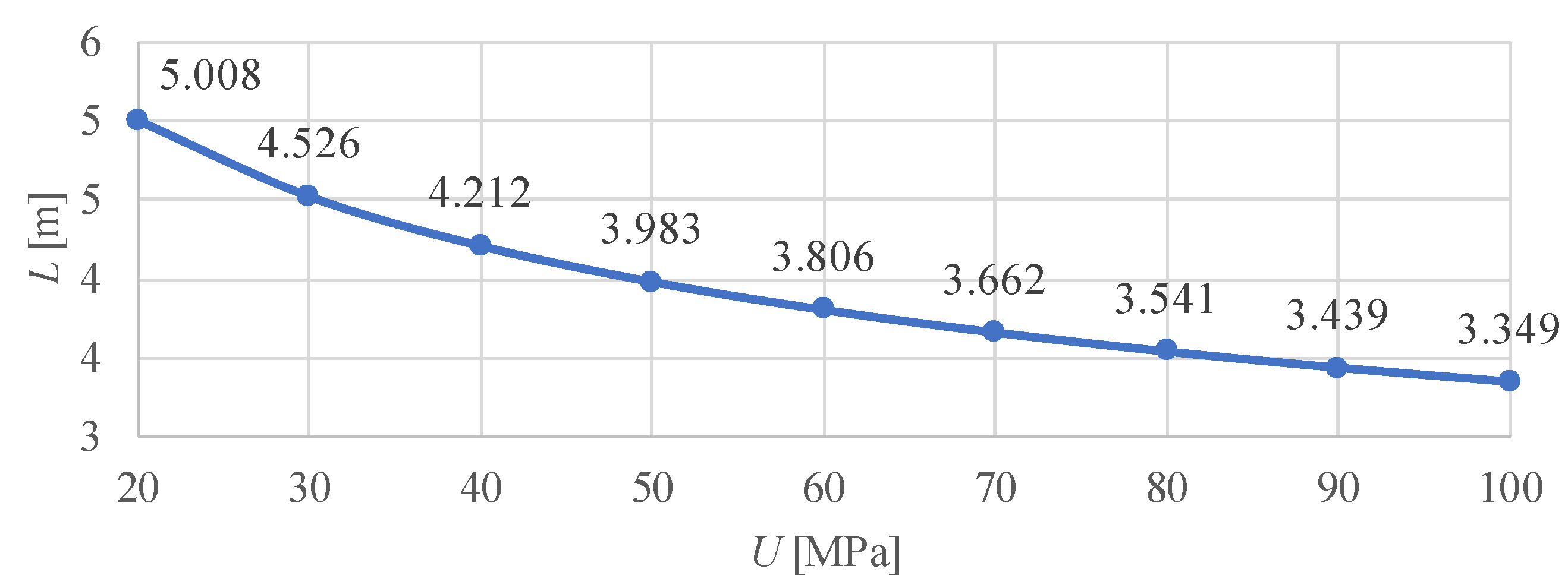
Hence, the rail deflection length depends on the track’s stiffness parameters. The deformation modulus of the sub-rail foundation can vary widely depending on the track structure (particularly the deformation moduli of the ballast layer and subgrade), its condition, and natural factors such as moisture and temperature [12]. The relationship between the calculated rail deflection length and this modulus is shown in Figure 2. The rail’s moment of inertia varies with rail type and wear, but its influence is minor and can be neglected for this purpose.
In some cases, even this length may prove insufficient. A low deformation modulus of the sub-rail foundation may result from poor ballast layer conditions (e.g., insufficient compaction, high contamination content, etc.) or inadequate subgrade strength. Such situations can become subjects of mathematical modeling aimed at investigating the consequences of degraded track conditions and/or substantiating appropriate reinforcement measures. This corresponds to a sub-rail foundation modulus of 50 MPa. For a “stiff” railway track, this length can be reduced, for example, to 3.4 m for a modulus of 100 MPa. For sections of a “softer” track, it can be increased, for example, to 4.5 m for a modulus of 30 MPa.
In cases where the stresses and deflections within the rail itself are not the focus of the study, it is feasible to create significantly shorter railway track models. For analyzing the stress–strain state of the sub-rail layers (ballast, subgrade), an adequate mathematical model can be obtained by applying an equivalent pressure directly to the investigated elements of the track structure.
The force transferred from the deflected rail to the sub-rail foundation (sleeper) can be determined analytically as a function of rail deflection in Equation (1) using the known relationship given by Equation (5):
Q = k l 2 P η
where l is the sleeper spacing; P is the wheel load applied to the rail.
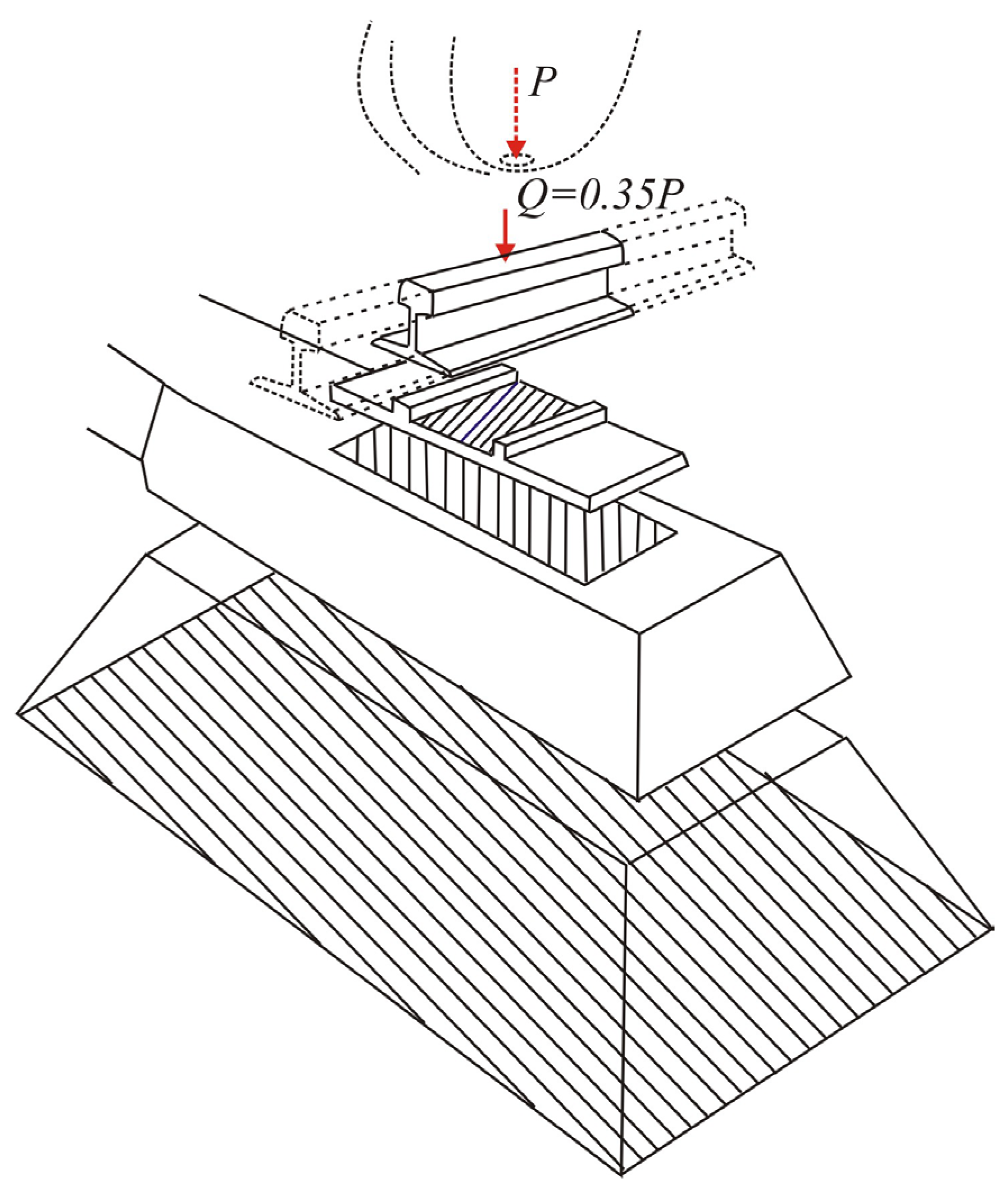
For a typical track structure with UIC60 rails, a sub-rail foundation modulus of 50 MPa, and a sleeper density of 165 per 100 m, it can be assumed that Q = 0.35 P . Thus, due to the load transfer through the deflected rail, the force transmitted to the sub-rail foundation will be approximately 35% of the wheel load applied to the rail.
It therefore makes sense to retain a “short” rail segment in the railway track model to generate realistic pressure from the sleeper base onto the rail fastening element and then onto the sleeper itself. However, when using a “short” rail, the load from the notional wheel must be reduced in accordance with Equation (5) (see Figure 3).

2.2. Number of Sleeper Units Along the Modeled Section

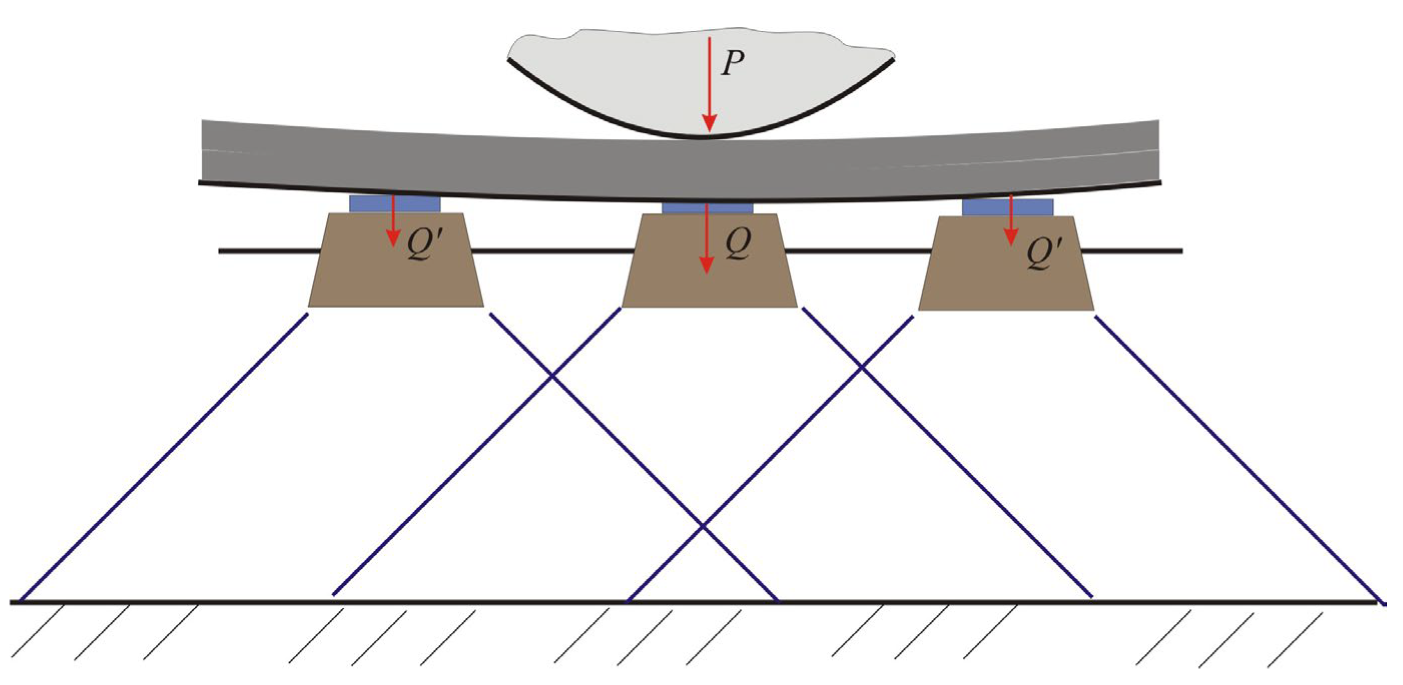
Depending on the sleeper spacing, the distance between sleeper centers typically ranges from 500 to 650 mm, and in some cases can vary even more widely. When the rail bends under the wheel load, it transmits the load not only to the central sleeper (located directly beneath the wheel contact point) but also to adjacent sleepers along the deflection length. The pressure exerted by the rail onto the sub-rail support (sleeper) can be determined analytically using Equation (5), taking into account that η = f ( x ) . The influence of the loads from neighboring sleepers begins to manifest at a certain depth within the ballast layer and continues into the subgrade. Generally, analytical calculations typically account for the load from three sleepers—the central sleeper and the two adjacent ones [35,36], as shown in Figure 4.
Accordingly, the load transfer from the rail to the sleepers, for further modeling of the stress–strain state of the sub-sleeper foundation, can be implemented in several ways, as illustrated in Figure 5.
Each of these options has its specific areas of application:
  • Option (a). The rail bends under the external load, and the deflection profile and amplitude determine the contact forces from the rail to the sleepers. This option most closely corresponds to the physical behavior of the system and, where possible, should be preferred over the others. However, its application has certain requirements. First, the rail length in the mathematical model must be sufficient to reproduce the ”complete” rail deflection with an appropriate profile and amplitude (see Section 2.1). Second, the model must include the necessary physical–mathematical tools to simulate not only compression (tension) but also bending.
  • Option (b). The rail is represented by notional short segments, with the pressure on each corresponding sleeper specified separately. This approach makes sense for models where the length of the railway track section is shorter than the full rail deflection length but long enough to include several sleepers. In this case, the external load can be specified as a distributed pressure on individual sleepers, as shown in Figure 3 and Equation (5).
  • Option (c). The rail transmits the load to the central sleeper only, while the loads on adjacent sleepers are neglected. This is reasonable for railway track models where the influence of adjacent sleepers on the stresses in the lower ballast layers and subgrade can be ignored. It should be noted that the use of very short models, whose length covers no more than one sleeper, does not automatically exclude the need to account for the additional pressure at the relevant depths beneath the sleeper foundation.

2.3. Shape and Dimensions of the Sub-Rail Domain

In the general approach of elasticity theory, the sub-rail foundation of a railway track (more precisely, the sub-sleeper foundation) is described as a half-space. Limiting the dimensions of the railway track model can be sufficient to produce a stress (or strain) distribution that deviates from what is expected for a true half-space. Considering the multilayered structure, anisotropy, and other properties characteristic of the railway track’s subgrade half-space, such an analysis requires the use of advanced contemporary mathematical models, such as the finite element method (FEM) and similar techniques. However, the use of complex mathematical models often obscures the root causes of such deviations. Therefore, for the analytical solution of the problem in this part of the study, the authors consider an isotropic medium. In Section 3 of the study, more sophisticated mathematical models are employed, in which the railway track is represented as a layered structure consisting of different elements with distinct physical properties.
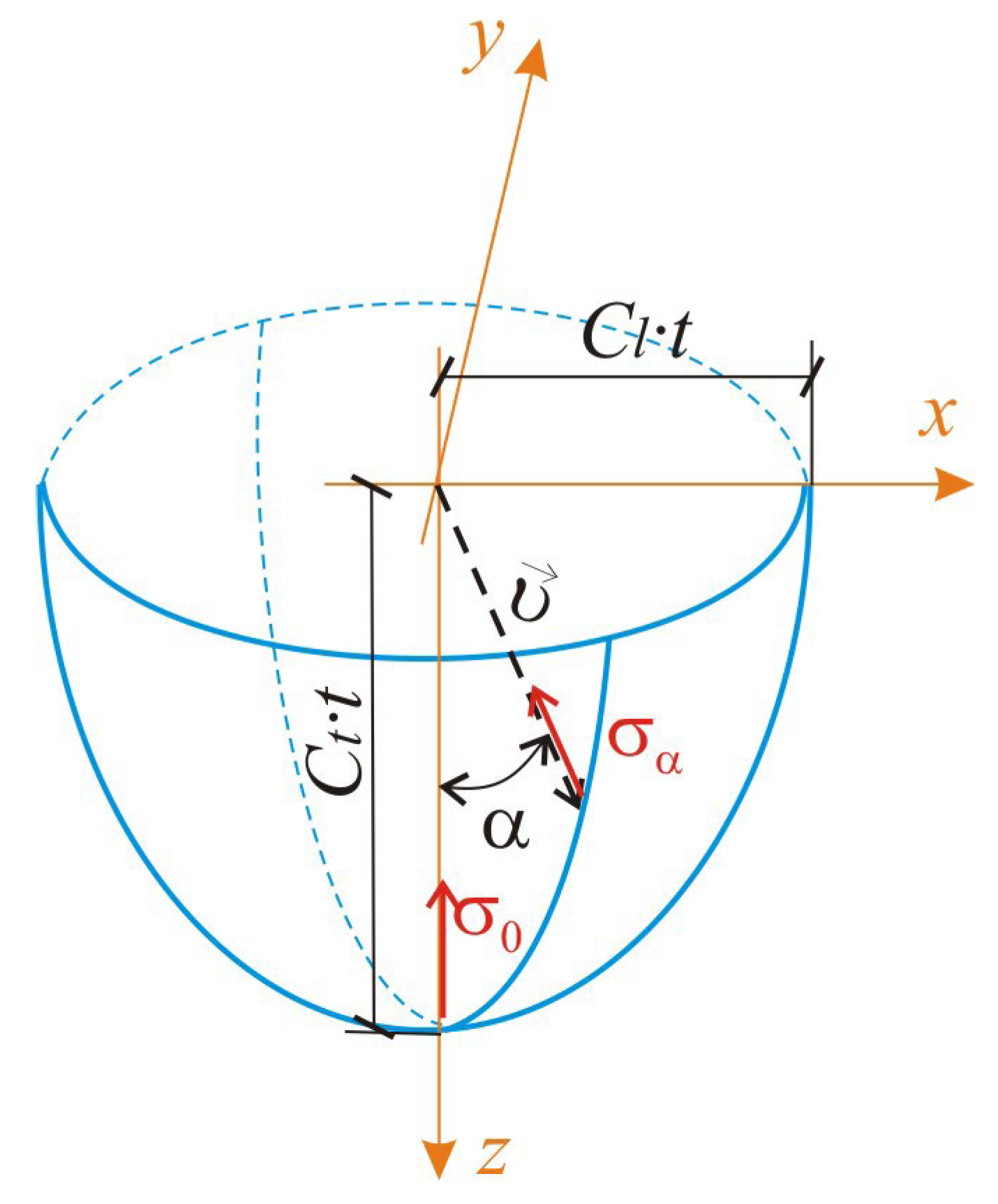
Let us consider the stress propagation in a half-space under a point load applied vertically, according to the classical Boussinesq problem. To derive the equations for stress propagation within the half-space, a number of assumptions are made: a three-dimensional space is considered in a Cartesian coordinate system; the force is applied at a point coinciding with the origin of coordinates; the direction of the force coincides with the z-axis; and the surface of the space that interacts with the force at time t corresponds to a set of points bounded by a surface forming the wave front [12,18], which can be described by ellipsoidal equations (Figure 6).
The longitudinal and transverse wave propagation velocities in a material are parameters that depend on its physical properties and can be determined using Equations (6) and (7):
C l = E 1 μ ρ 1 + μ 1 2 μ ;
C t = E 2 ρ 1 + μ ,
where E is Young’s modulus; μ is Poisson’s ratio; and ρ is the material density.
The geometric position of the points on the ellipsoidal surface (see Figure 6) is defined by the vector length in the direction α :
υ = t C α
where C α is the wave propagation velocity in the spatial direction α :
C α = C t C l C t 2 cos 2 α + C l 2 sin 2 α .
or equivalently,
C α = φ C l φ 2 + 1 φ 2 sin 2 α .
where
φ = C t C l = 1 2 μ 2 1 μ .
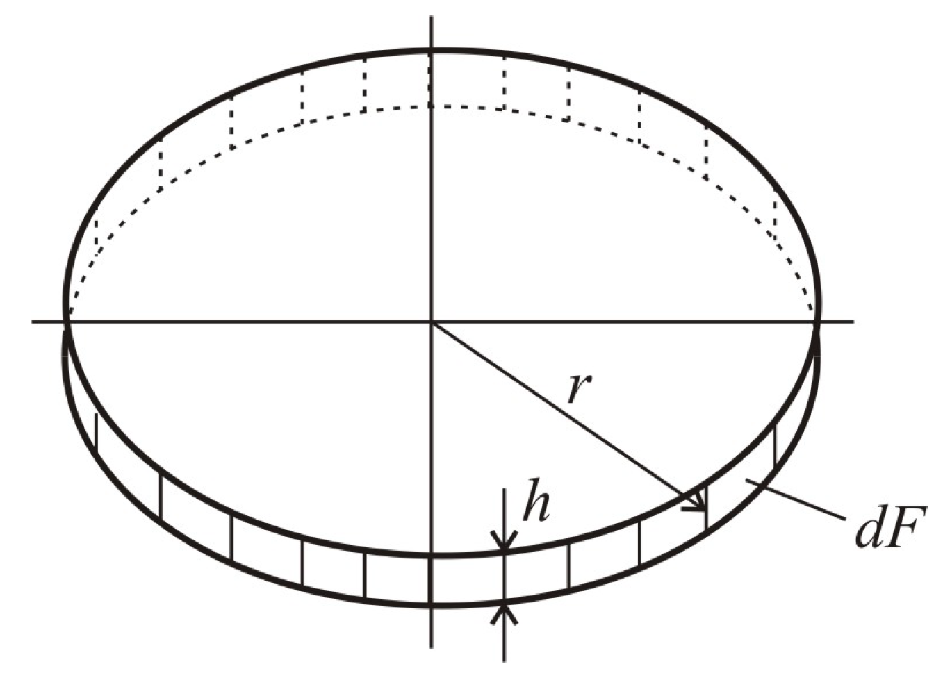
It is assumed that the surface in the space consists of discrete rings, whose radii vary according to Equation (12); see Figure 7:
r = C α t sin α ,
where α is the angle defining the position of a point on the surface, with α 0 ; π / 2 for a complete ring.
The area of such a ring is defined by Equation (13):
d F α = 2 π r h ,
where h is the nominal thickness of the ring:
h = C α t d α .
Taking Equations (12) and (14) into account, the area of the computational ring is then given by Equation (15):
d F α = 2 π C α 2 t 2 sin α d α .
In general, for any surface cut from a half-space in equilibrium under a concentrated force P , the equilibrium condition must satisfy Equation (16):
P = 0 π 2 σ α cos α d F α .
The relationship between the stresses acting on the horizontal plane of the computational surface in an arbitrary direction α ( σ α ) and the stresses aligned with the axis of force application α = 0 ( σ 0 ) is given by Equation (17); see Figure 6:
σ α = σ 0 C l 2 cos α C α 2 .
After mathematical transformations, considering Equations (15) and (17), the equilibrium condition (16) becomes the following:
P = 2 π C l 2 t 2 σ 0 0 π 2 cos 2 α sin α d α .
Given that 0 π 2 cos 2 α sin α d α = 1 3 , and denoting the computational depth as z = C l t , the solution yields the well-known Boussinesq equation for determining stress at a point on the load axis:
σ 0 = 3 P 2 π z 2 .
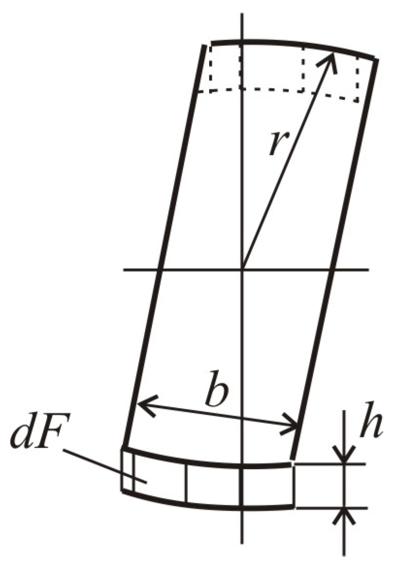
For short railway track models (see Figure 8), the computational elementary area (Figure 7) transforms into the domain shown in Figure 9.
Accordingly, for a bounded domain of length b (see Figure 9), assuming b < r , Equation (13) takes the following form:
d F α = 2 b h .
The equilibrium Equation (16), after mathematical transformations with consideration of Equations (10), (14), (17) and (20), can be written as follows:
P b = 2 σ 0 z b 1 φ 0 π 2 c o s 2 α φ 2 + 1 φ 2 s i n 2 α d α .
After numerically solving the integral for μ = 0.3 (see Equation (11)) and bringing the result into a form analogous to Equation (19), the following result is obtained:
σ 0 b = P 1.646 z b .
The influence of the model length b can be analyzed through the stress ratio at depth z:
k = σ 0 b σ 0 = 1.272 z b .
Equation (22) shows that even under a basic elasticity formulation—i.e., determining the vertical stress in an isotropic half-space along the axis of a single concentrated force—the stress level depends not only on the depth but also on the size of the bounded domain (b). If the stress level is compared to that of a conditionally unbounded half-space, it will be higher by a factor of k (Equation (23)). It should be noted that this coefficient k is not constant with depth. This fact, along with the significant simplification of the computational scheme (Figure 6) compared to the real multilayer structure of a railway track, makes it impractical to compensate for the bounded domain by simply reducing the external load by this factor. However, this insight helps to better understand the occurrence of overestimated stress levels under certain modeling configurations.

3. Results of Mathematical Modeling

The influence of the railway track length introduced into the mathematical model was analyzed using two different mathematical approaches: modeling the railway track through the propagation of elastic waves and finite element modeling. The propagation of stresses and deformations within the railway track domain—specifically within the ballast layer and the subgrade—was studied for various length constraints of the railway track, considering the different boundary condition approaches discussed in the previous section.
For the calculations, a railway track structure with UIC60 rails, reinforced concrete sleepers, and crushed stone ballast was adopted, which is currently typical for most mainline railway sections. The principal physical characteristics of the track components are presented in Table 1.
The external load was modeled as a single quasi-static point force of 100 kN applied vertically along the rail head axis. For some problems, it is possible to consider a sequence of forces corresponding to the wheel loads from a bogie, or to increase the value of the single force by accounting for the combined action of several wheels, considering the distance between them. A quasi-static representation of the force can also be ensured by increasing the static load with appropriate dynamic coefficients that reflect train speed, rolling stock type, and other factors [35].

3.1. Modeling the Railway Track Through the Propagation of Elastic Waves

Figure 10 illustrates the computational models employed to calculate stress distribution within the railway track domain for two configurations with significantly different lengths: 9.0 m and 0.2 m. The 9.0 m configuration features a full rail–sleeper system with 17 sleepers and has been validated in a series of previous studies conducted by the authors [12]. A track length of 9 m can be considered more than sufficient under the previously discussed conditions and is therefore used as the reference case for further analysis.
A specific feature of a railway track model of this class [35] is the formation of the computational domain interacting with the applied load through the step-by-step propagation of an elastic wave. The determination of the wave front accounts for the geometrical outlines of the objects and their physical characteristics, in particular those that define wave velocity. The stress–strain state of such a medium is obtained by solving a system of differential equations that describe the transfer of pressure within it as the wave propagates. In this case, the rail deflection is formed as a result of the deformation of the multilayered sub-rail foundation [12,18].
The shortest configuration analyzed has a length of 0.2 m, which is shorter than the typical width of a concrete sleeper. For this and other models containing less than one sleeper length—and thus unable to account for the elastic bending of the rail—the external force was reduced to 35 kN (see Equation (5) and Figure 3).
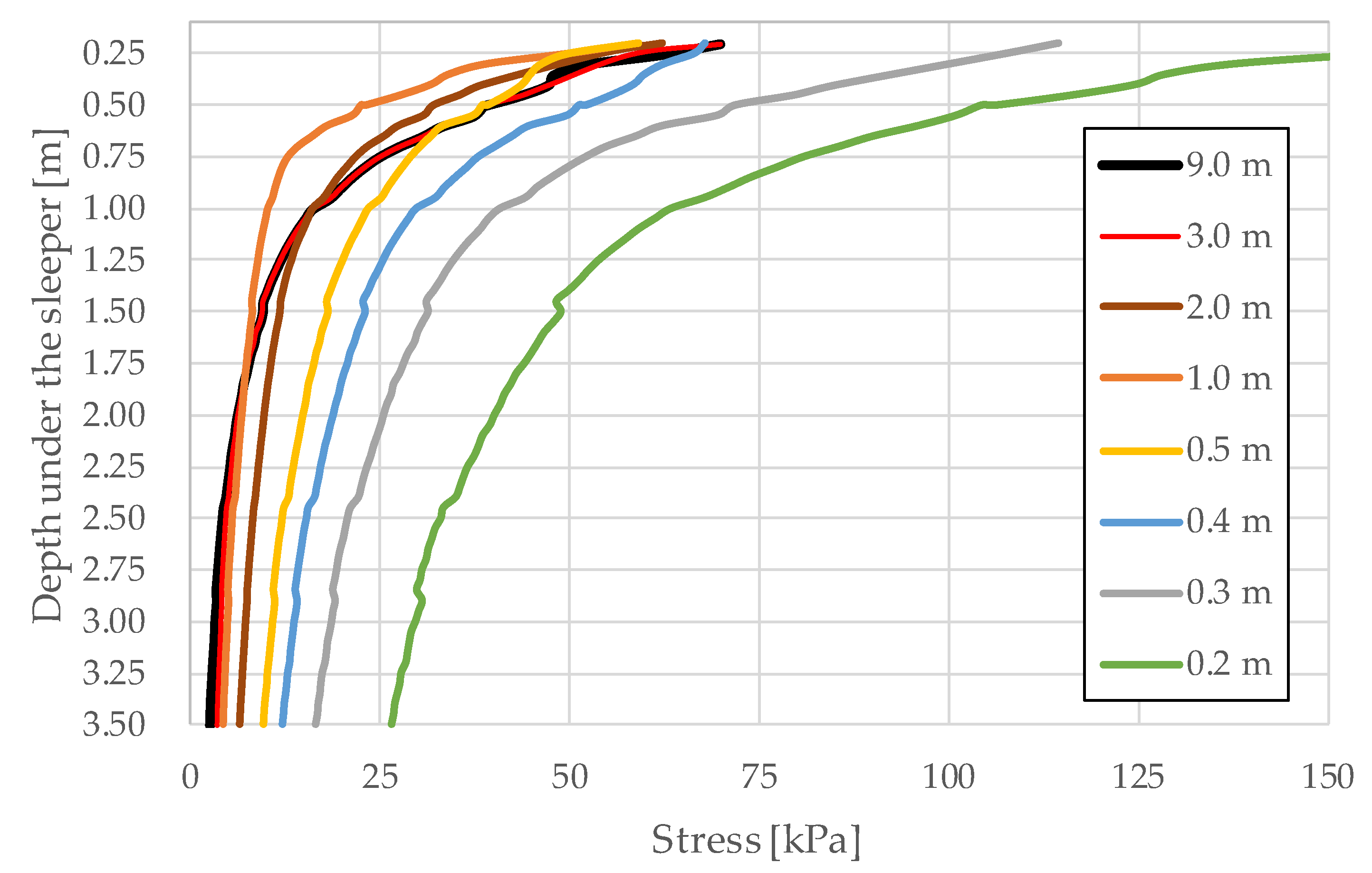
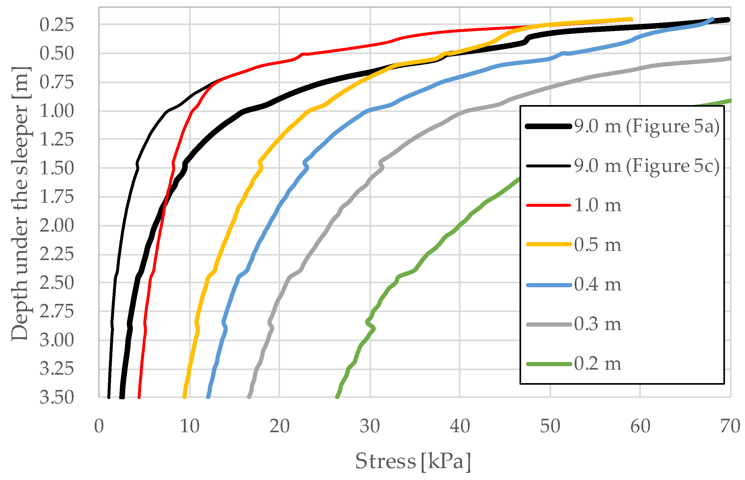
For a detailed comparison, the stress distribution was further analyzed only along the rail axis (the axis of the applied external force). Figure 11 shows the variation in vertical stresses in the sub-sleeper foundation: up to 0.5 m—the ballast layer; below—the subgrade soil. Several cases are presented for models with track lengths ranging from 0.2 m to 9.0 m.
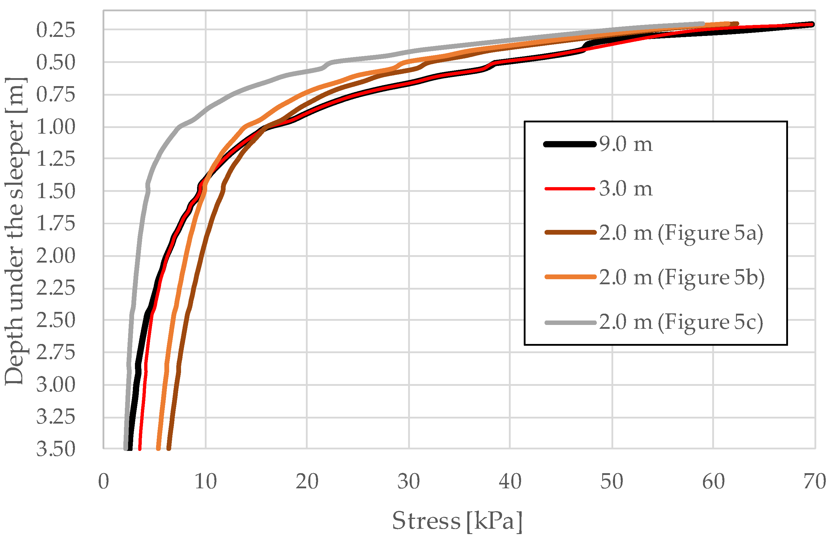
With a gradual increase in model length, a decrease in calculated stress levels is observed, which can be explained by the increase in material volume that absorbs the external load. The change in this trend for models of 2.0 m length and longer is due to the fact that such models include more than one sleeper, and thus the pressure on the ballast (and subsequently on the subgrade) from the “central” sleeper is supplemented by the pressure from adjacent sleepers. Figure 12 shows the calculation results for cases up to and including 1.0 m in length (containing one sleeper only). For comparison, the 9.0 m configuration is shown in both the full reference version and a variant where the track structure was defined with only one sleeper and a short rail fragment (see Figure 5c).
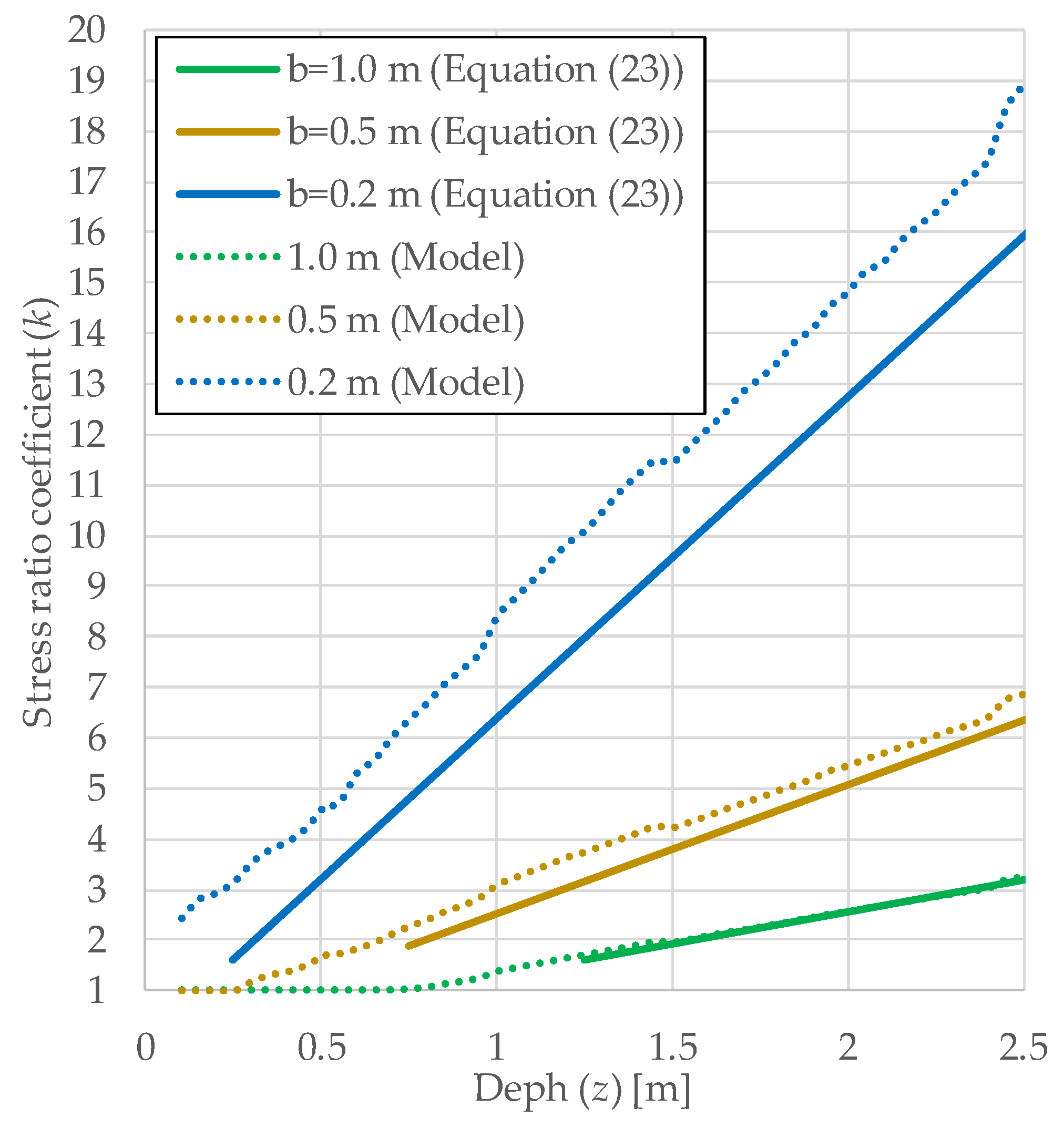
To evaluate the influence of the constrained sub-sleeper domain using the method described in Section 2.3, Figure 13 shows the calculation results according to Equation (23) alongside the results for the ratio of stresses determined for models with a defined limited length to the stresses in the 9.0 m model containing only one sleeper.
A sufficiently close match of the results shown in Figure 13 demonstrates that the main reason for the increase in calculated stresses when using short models—under the condition of identical loading—is the spatial constraint on the elastic domain that absorbs and propagates the stresses (see Figure 9). The higher stress values obtained for the 0.2 m variant—even compared to those predicted by Equation (23)—are expected and can be explained by the fact that in this case the width of the domain does not exceed the width of the load footprint (i.e., the sleeper base width). From the perspective of elasticity theory, this effectively shifts the problem from the class of semi-infinite elastic body deformation to the class of plate elasticity problems.
Further increasing the model length enables the inclusion of multiple sleepers, allowing for a more realistic representation of how the load is transferred from the rail through the sleepers to the ballast. However, if the rail length is still insufficient to develop the full bending behavior, such load transfer may require appropriate correction (see Figure 14).
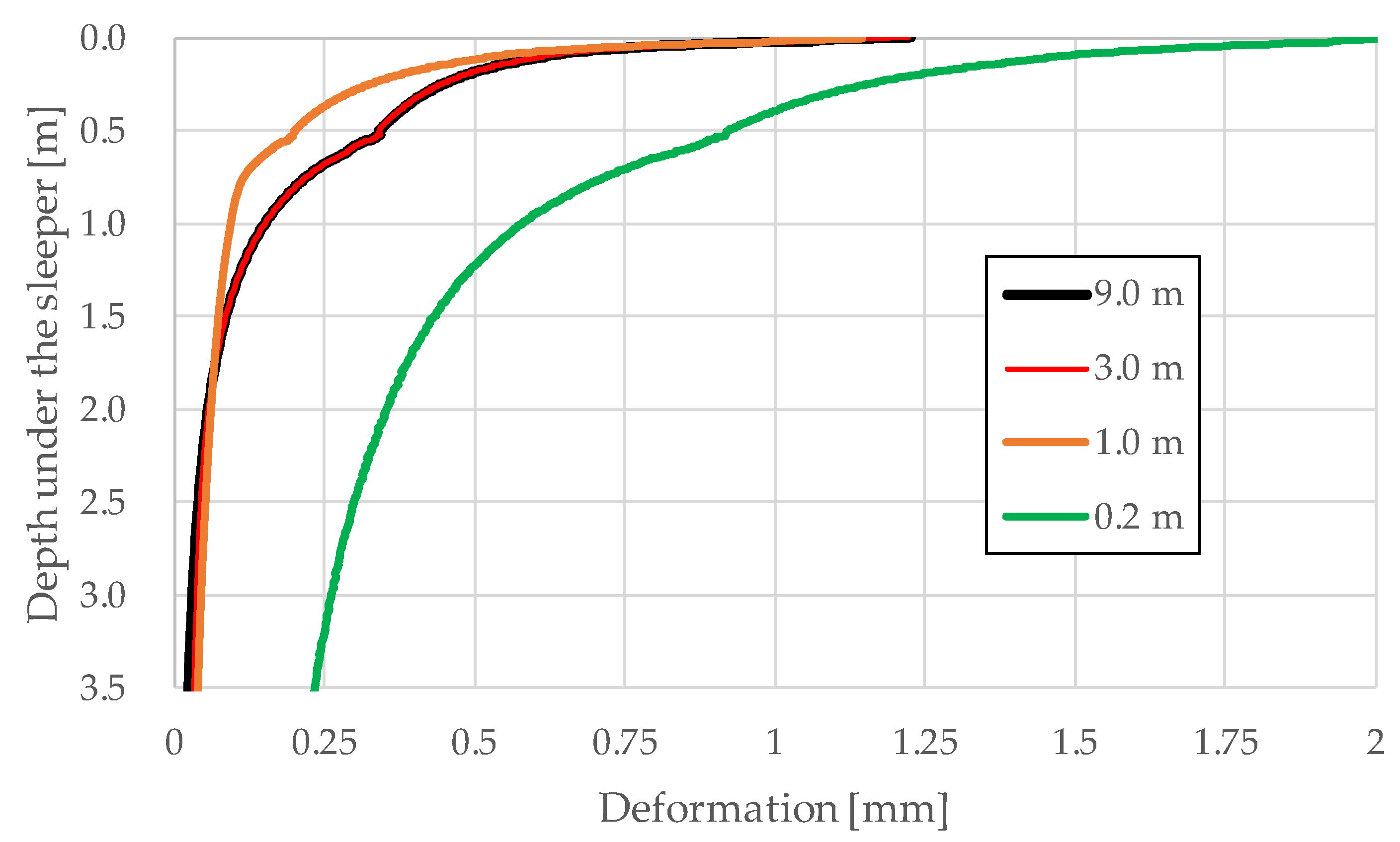
Figure 15 shows the results for rail deflections for the main modeling variants.
The calculated deflections (absolute deformations along the axis of the applied load) together with the stresses are a key indicator for interpreting the system’s behavior. In particular, the deformations serve as a clear and practical criterion for verifying whether a fully developed deformation state has formed.

3.2. Finite Element Modeling

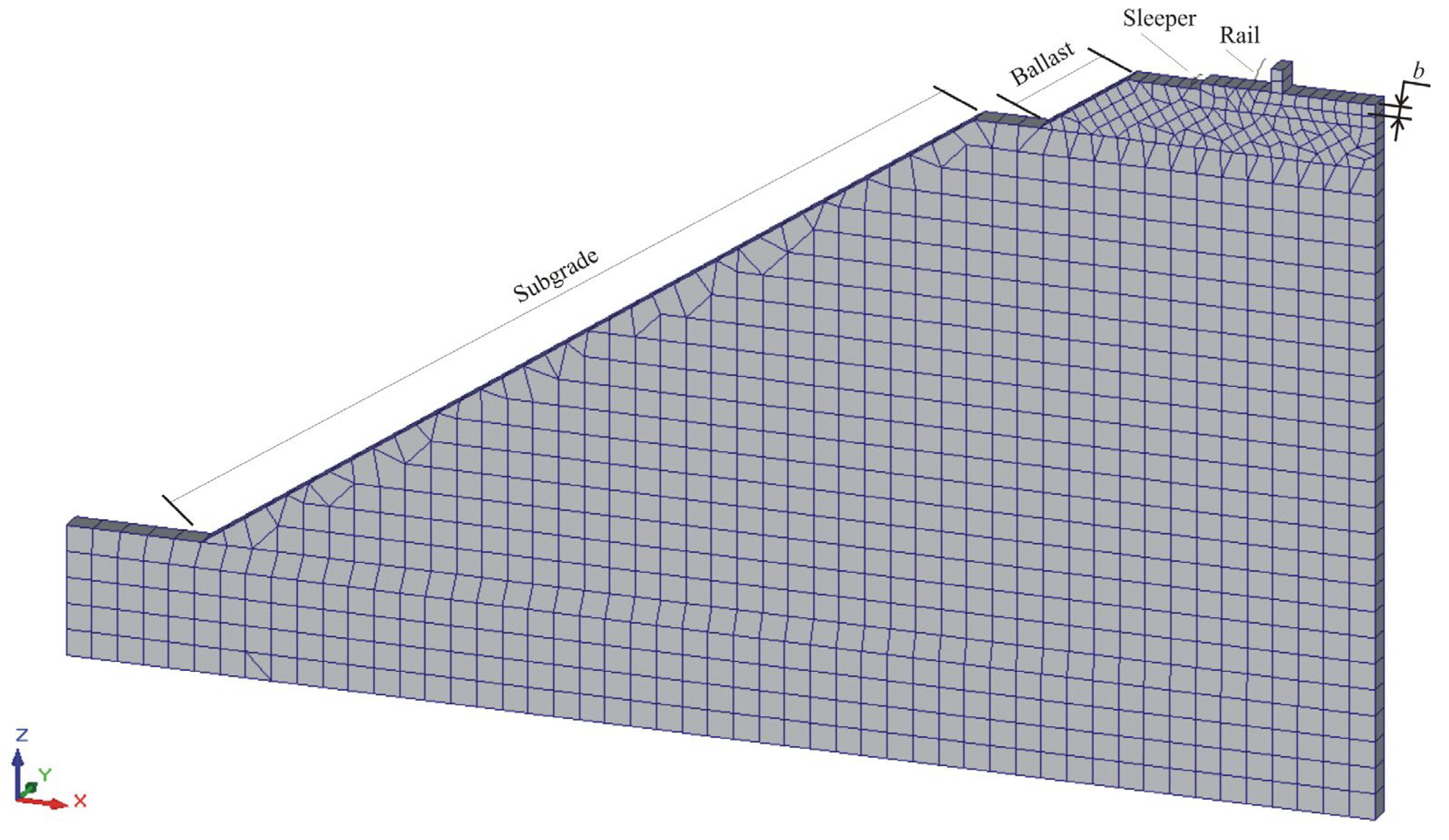
To investigate the influence of the size of the finite element model and the boundary conditions imposed on it, a numerical analysis was conducted for six finite element models of the subgrade with a height of 4.0 m. The base geometry for all the finite element models was the one shown in Figure 8, with the model characteristics as given in Section 3.1. The problem was set up in three dimensions. Accordingly, the finite elements used were solid prisms and tetrahedra (the latter accounting for no more than 5–7% of the total number of elements in the models).
Key preliminary observations regarding the impact of boundary conditions are as follows. If the lateral boundaries are left free, this is equivalent to modeling a confined plate rather than a semi-infinite half-space. As a result, the calculated stresses—especially in the central zone—will be overestimated due to edge compression effects.
Some implementations of the finite element method offer artificial tools to partially compensate for this effect. One option is to use special elastic supports (elastic foundation or spring supports), which allow the edges to move slightly while avoiding rigid clamping. This can partially reduce edge effects.
Some commercial software packages (such as ABAQUS, ANSYS) also allow the use of infinite elements (infinite elements or absorbing boundaries). These special elements dampen the stresses at the boundaries, simulating the continuation of the domain into infinity.
Another tool is non-reflecting boundary conditions (absorbing boundaries or non-reflecting boundaries). Non-reflecting conditions “transmit” the stresses through the boundary as if the domain extended further. Such approaches help to reduce boundary effects and their impact on the deformed state of the railway track domain.
Based on the real operating conditions of the railway subgrade, it is known that the upper part of the system (the rail–sleeper assembly and the upper part of the ballast) as well as the embankment slopes are free from any restraints. Therefore, boundary conditions must not be applied to these surfaces of the finite element model.
A logical step in assigning boundary conditions to the geometry is to consider that the finite element model represents only a portion of the subgrade, which has a certain length. Therefore, the end faces of the model should be constrained along the track axis solely by one boundary condition (y = 0, plane strain condition), allowing the model to deform freely in the vertical (z) and transverse (x) directions. With a correctly chosen model length, as will be shown below, this boundary condition does not affect the distribution of the stress–strain state components.
An important boundary condition is the constraint along the horizontal axis (x = 0) on the end face along the axis of symmetry that appears in the model after halving it. In this case, vertical and longitudinal deformations are not restricted (z ≠ 0, y ≠ 0) and can freely propagate within the model.
To minimize edge effects and their impact on the deformed state of the subgrade, a soil foundation with dimensions of 1.0 × 1.0 m was modeled beneath the subgrade. Its sides are constrained against horizontal and longitudinal deformations (z ≠ 0; x = y = 0), and its bottom surface is fully constrained against horizontal, longitudinal, and vertical deformations (x = y = z = 0).
The listed boundary conditions, in particular the fixation of the lower surface of the model in all degrees of freedom, the symmetry conditions which allow the dimensionality of the problem to be reduced without distorting the results, and the special tools embedded in FEM implementations (absorbing boundaries, elastic supports, etc.), are widely applied in modern studies, e.g., [1,3,5], and can already be considered classical.
Thus, the finite element models consider the portion of the system excluded by the symmetry condition as well as the plane strain condition that arises at the end faces of the model “cut” from a larger system, while still allowing the stress–strain state components to distribute freely, provided the discretization is adequate.
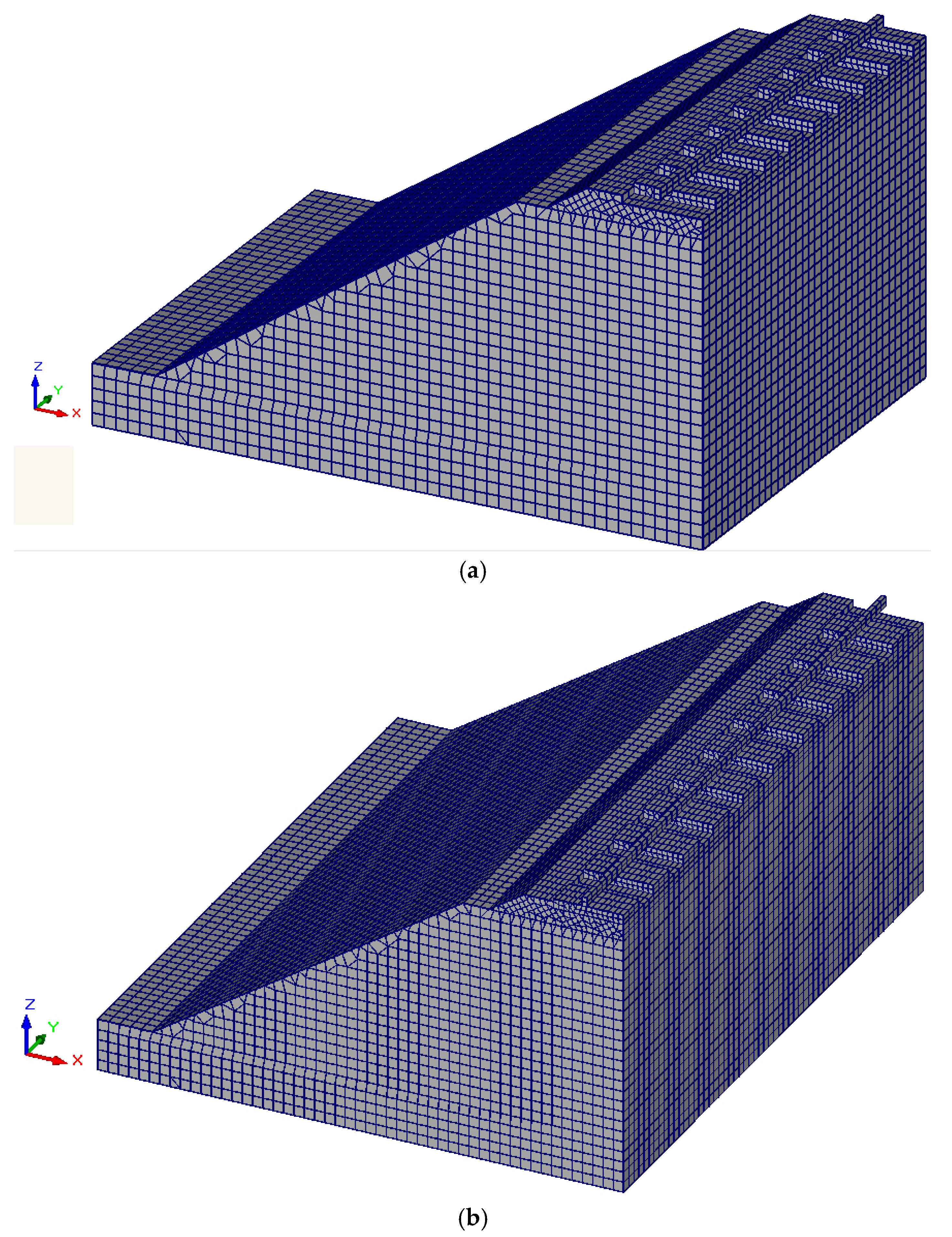
To investigate the influence of mesh size, number of finite elements, and model length, variations in the discretization of the subgrade and soil foundation were carried out. In all models, the rail, sleeper, and ballast layer were discretized using elements with dimensions of 0.1 × 0.1 × 0.1 m. This practical step in modeling is explained by the fact that finite element method recommends reducing the element size in areas subjected to point loads. Many fundamental works devoted to this numerical method emphasize that increasing the size of the finite element mesh is appropriate in parts of the model that are further from the point of load application. For the subgrade, three types of finite element meshes were used with element sizes of 0.1 × 0.1 × 0.1 m, 0.2 × 0.2 × 0.2 m, and 0.5 × 0.5 × 0.5 m, respectively. Accordingly, for these meshes, the length of the model was chosen to be a multiple of the element size: 0.2 m (Figure 8); 1.0 m; and 7.2 m.
For the third mesh, the results of the deformed state are not provided in order to save space in the manuscript and because such an element size does not provide the required calculation accuracy (a simulation with a mesh of 1.0 × 1.0 × 1.0 m was planned but was not carried out, since the analysis of the third mesh showed it to be entirely unsuitable). Therefore, the detailed analysis of the deformed state, the results of which are presented below, was carried out for two meshes with element sizes of 0.1 × 0.1 × 0.1 m and 0.2 × 0.2 × 0.2 m, with model lengths of 0.2 m and 7.2 m, respectively (Figure 16a); for the mesh with an element size of 0.2 × 0.2 × 0.2 m, a model with a length of 12.0 m was also developed (Figure 16b).
The discretization parameters for these models are as follows: 7244 finite elements and 11,160 nodes (mesh 0.1 × 0.1 × 0.1 m, length 0.2 m); 36,540 finite elements and 39,367 nodes (mesh 0.2 × 0.2 × 0.2 m, length 7.2 m); and 64,785 finite elements and 60,900 nodes (mesh 0.2 × 0.2 × 0.2 m, length 12.0 m). After the finite element models were created, calculations were performed using the StructureCAD suite, and the results are analyzed further below (Figure 17). The railway model was built using Structure CAD for Windows, version 7.29 R.3 (SCAD) (license number F755B84 (KMBKB RA 4810)).
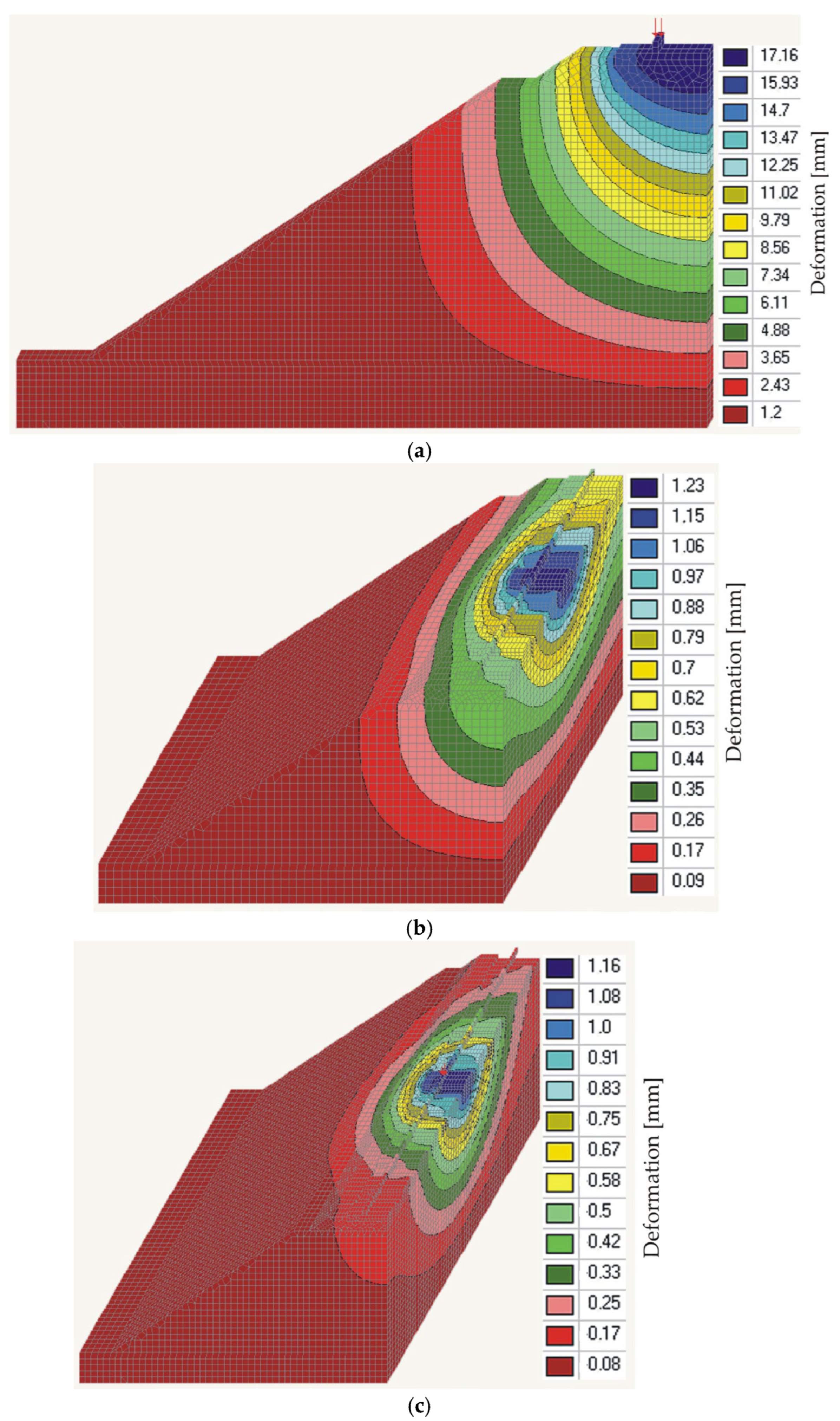
The first observation arising from the analysis of the deformed state of the three models is the fundamentally different value of the maximum vertical component in the first model compared to the second and third models, as it differs by an order of magnitude: 17.16 mm in the finite element model with a length of 0.2 m, versus 1.23 mm and 1.16 mm in the models with lengths of 7.2 m and 12.0 m, respectively. This phenomenon can be explained by the fact that the model with a length of 0.2 m corresponds to the condition of a “short” rail; that is, the model length is insufficient for the free distribution of the deformed state. To obtain deformations in such a “short” rail model that are representative of the normal situation of a moving load, the applied load must be reduced, as shown above.
Qualitatively, the deformation behavior of the 0.2 m model (Figure 17a) resembles the behavior of a strip foundation. This is an objective situation because in such a short model, even a single sleeper does not fully fit within its width. Accordingly, the rail–sleeper grid, which acts as a beam grillage rather than a foundation, is modeled here in a truncated form. This statement is easily supported by examining the deformed state of the models with lengths of 7.2 m (Figure 17b) and 12.0 m (Figure 17c).
As can be seen from Figure 17, the vertical component of the deformed state is influenced to a greater extent by the model length rather than by the discretization. The model, with a length of 0.2 m, uses a mesh that is twice as fine as that of the other two models; however, its length does not allow the deformed state to develop fully. In the model with a length of 7.2 m, the deformed state is formed more freely (Figure 17b); however, it can be observed that the model’s edge “cuts off” part of the isolines and isofields of vertical deformations. Comparison of this model with the 12.0 m long model (Figure 17c) definitively confirms this fact.
However, even in the model with a length of 12.0 m, it can be observed that the bright red deformation field is “cut off” by the model’s edge. Nevertheless, further increasing the model length can be considered impractical for a clear reason: the deformed state in a finite element model can be assumed to be fully formed if the calculation domain contains an isoline corresponding to 10% of the maximum deformation. In this specific case, the isoline with a value of approximately 0.12 mm is not directly displayed by the analysis software, but it can be roughly determined by interpolating between the 0.17 mm and 0.08 mm isolines. This isoline lies within the bright red field, indicating that it is within the computational domain, which suggests that the chosen model length is appropriate. For the 7.2 m long model, a similar isoline at about 0.12 mm is “cut off” by the model’s end, so its length needs to be increased, which was performed in the 12.0 m model.
Based on the analysis of the rail–sleeper grid deflection in the 12.0 m long model, it was found that the length over which active deformation occurs (with the limit of such deformation taken as 10% of the maximum displacement at the point of applied load) is about 9.0 to 9.4 m, which is very close to the length determined earlier in Section 3.1. To fully match the analytical solution, a parametric analysis of the 12.0 m finite element model should be conducted with varying deformation moduli of the different parts of the system. However, the numerical results obtained so far are in sufficient agreement with the analytical solution.

4. Discussion

The results of this study confirm that the model length and boundary conditions are critical factors in the development of mathematical models of railway track structures. Insufficient dimensions of the computational domain, particularly in the longitudinal direction, significantly limit the ability of the stress–strain state to propagate, resulting in overestimated stress and deformation values fully. This effect was observed both when using the wave propagation approach and in numerical analyses based on the finite element method.
An analytical assessment of rail deflection enabled the determination of the characteristic length of the influence zone, which depends on the stiffness of the rail–sub-rail system. This means that a model shorter than this length cannot reproduce the full rail deflection and therefore cannot realistically transfer loads to the sleepers and further to the ballast and subgrade.
Special attention should be given to the number of sleepers included in the model. Although analytical calculations indicate that the main load is distributed across three sleepers (the central sleeper and two adjacent ones), several possible simplifications are possible. In particular, a model can either fully reproduce the rail deflection (which is physically the most realistic approach) or implement an approximate load transfer without considering bending. As the results demonstrate, the latter approach can be acceptable for local models but requires appropriate load scaling.
The analysis of the shape of the sub-rail domain showed that shortening the model length disturbs the stress transfer conditions within the semi-infinite space. This appears as elevated stresses, especially near the point of load application. The proposed analytical method enables the estimation of the effect of this limitation, although its application to multilayered and anisotropic media remains constrained.
The results of the finite element modeling confirmed that the key factor for calculation adequacy is the model length itself, rather than only the mesh resolution. In particular, even with high mesh refinement (0.1 m), the short model (0.2 m) exhibited deformations that do not accurately reflect the real behavior of the track structure. By contrast, the models with lengths of 7.2 m and 12.0 m allowed the deformed state to develop fully, and the use of the 10% maximum deformation isoline as a practical criterion for completing the influence zone proved to be practical and reasonable.
At the same time, excessively long models result in unjustified increases in computational cost. Therefore, a balanced approach to choosing the model length and boundary conditions is required. Short models are not inherently incorrect, but they demand careful adjustment of the applied loads and boundary constraints to ensure reliable results. Future research may focus on developing unified methods for load scaling and constructing transition models that adapt short models to full-space conditions [37].

5. Conclusions

This study substantiates the importance of selecting an appropriate model length and applying suitable boundary conditions when developing mathematical models of railway track structures. The results demonstrate that an insufficiently sized domain, especially in the longitudinal direction, can significantly distort the stress–strain state due to the limited spread of deformations. Conversely, excessively large domains may reduce computational efficiency without adding accuracy.
Through an analysis based on elastic wave propagation and finite element modeling, it was demonstrated that the model length must be sufficiently long to capture the spatial distribution of deformations caused by vertical loads. In particular, models shorter than the effective rail deflection length (approximately 4–9 m, depending on the subgrade stiffness) require load scaling or additional assumptions to yield realistic results. Otherwise, they tend to overestimate stress and deformation levels.
Based on the full rail deflection implementation, the minimum longitudinal length of the model can be recommended as 3.4, 4.0, and 4.5 m for sections with a sub-rail foundation modulus of 100, 50, and 30 MPa, respectively.
The finite element analysis confirmed that for a subgrade with a height of 4.0 m, an element size of 0.2 × 0.2 × 0.2 m provides an adequate level of discretization to obtain reliable deformation results. The recommended boundary condition scheme for a half-space model of the subgrade is as follows: (i) the upper part (the rail–sleeper grid and the top ballast layer) and the slopes remain free of any restraints; (ii) the model ends are assigned a plane strain boundary condition along the track axis (y = 0), allowing vertical (z) and transverse (x) deformations; (iii) ties are applied along the horizontal axis (x = 0) at the symmetry plane, while vertical and longitudinal deformations remain unconstrained (z ≠ 0; y ≠ 0); (iv) the foundation beneath has side constraints that prevent horizontal and longitudinal deformations (z ≠ 0; x = y = 0); and the bottom plane is fixed against all displacements (x = y = z = 0).
It was also found that to adequately transfer stresses through the sleepers, at least three sleepers should be included in the model. For very short models, appropriate corrections to the applied loads, based on analytical relationships, are necessary to ensure consistency with full-scale behavior [38].
Furthermore, it was demonstrated that the use of suitable boundary conditions, especially on lateral and bottom surfaces, is crucial to avoid artificial constraints. Strategies such as symmetry conditions, absorbing boundaries, and elastic supports can improve the realism of simulations while minimizing computational demands.
These findings can assist in developing optimized, computationally efficient railway track models that remain physically accurate and robust under a wide range of geotechnical and structural conditions.

Author Contributions

Conceptualization, S.F. and M.K.; methodology, D.K.; validation, S.F., D.K. and O.T.; formal analysis, S.F., M.K. and O.T.; writing—original draft preparation, S.F., D.K., M.K. and O.T.; writing—review and editing, S.F., D.K., M.K. and O.T.; visualization, D.K. and O.T.; project administration, S.F. All authors have read and agreed to the published version of the manuscript.

Funding

This research received no external funding.

Institutional Review Board Statement

Not applicable.

Informed Consent Statement

Not applicable.

Data Availability Statement

Data are contained within the article.

Acknowledgments

The authors express gratitude to the employees of the Ukrainian State University of Science and Technologies and the members of the “SZE-RAIL” research team and the Vehicle Industry Research Center at Széchenyi István University. This research was supported by the SIU Foundation’s project ‘Sustainable Railways—Investigation of the energy efficiency of electric rail vehicles and their infrastructure’. The publishing of the paper did not receive financial support or financing for the article process charge.

Conflicts of Interest

The authors declare no conflicts of interest.

References

  1. Alkhdour, A.; Tiutkin, O.; Fischer, S.; Kurhan, D. An Analytical Method for Determining the Stress–Strain State of a Subgrade with Combined Reinforcement. Infrastructures 2024, 9, 240. [Google Scholar] [CrossRef]
  2. Petrenko, V.; Bannikov, D.; Kharchenko, V.; Tkach, T. Regularities of the deformed state of the geotechnical system “soil base—Micropile”. IOP Conf. Ser. Earth Environ. Sci. 2022, 970, 12028. [Google Scholar] [CrossRef]
  3. Jankowski, W.; Sołkowski, J. The modelling of railway subgrade strengthening foundation on weak soils. Open Eng. 2022, 12, 539–554. [Google Scholar] [CrossRef]
  4. Alsirawan, R.; Koch, E.; Alnmr, A. Proposed Method for the Design of Geosynthetic-Reinforced Pile-Supported (GRPS) Embankments. Sustainability 2023, 15, 6196. [Google Scholar] [CrossRef]
  5. Alsirawan, R.; Koch, E. The finite element modeling of rigid inclusion-supported embankment. Pollack Period. 2022, 17, 86–91. [Google Scholar] [CrossRef]
  6. Deng, Y.; Zhao, H.; Li, L.; Yao, Z.; Li, L. Research on static and dynamic loading performance of geosynthetic reinforced and pile-supported embankment. Appl. Sci. 2023, 13, 3152. [Google Scholar] [CrossRef]
  7. Guo, Q.; Li, B.; Ye, Z.; Xu, J. Finite Element Analysis on the Behavior of Solidified Soil Embankments on Piled Foundations under Dynamic Traffic Loads. Appl. Sci. 2024, 14, 4464. [Google Scholar] [CrossRef]
  8. Alsirawan, R.; Koch, E. Dynamic analysis of geosynthetic-reinforced pile-supported embankment for a high-speed rail. Acta Polytech. Hung. 2023, 21, 31–50. [Google Scholar] [CrossRef]
  9. Chango, I.V.L.; Yan, M.; Ling, X.; Liang, T.; Assogba, O.C. Dynamic response analysis of geogrid reinforced embankment supported by CFG pile structure during a high-speed train operation. Lat. Am. J. Solids Struct. 2019, 16, e214. [Google Scholar] [CrossRef]
  10. Feng, G.; Luo, Q.; Lyu, P.; Connolly, D.P.; Wang, T. An Analysis of Dynamics of Retaining Wall Supported Embankments: Towards More Sustainable Railway Designs. Sustainability 2023, 15, 7984. [Google Scholar] [CrossRef]
  11. Giner, I.G.; Alvarez, A.R.; Sánchez-Cambronero García-Moreno, S.; Camacho, J.L. Dynamic modelling of high-speed ballasted railway tracks: Analysis of the behaviour. Transp. Res. Procedia 2016, 18, 357–365. [Google Scholar] [CrossRef]
  12. Kurhan, D.; Fischer, S. Modeling of the Dynamic Rail Deflection using Elastic Wave Propagation. J. Appl. Comput. Mech. 2022, 8, 379–387. [Google Scholar] [CrossRef]
  13. Xie, H.; Luo, Q.; Wang, T.; Jiang, L.; Connolly, D.P. Stochastic analysis of dynamic stress amplification factors for slab track foundations. Int. J. Rail Transp. 2024, 12, 281–303. [Google Scholar] [CrossRef]
  14. Xu, F.; Yang, Q.; Liu, W.; Leng, W.; Nie, R.; Mei, H. Dynamic stress of subgrade bed layers subjected to train vehicles with large axle loads. Shock Vib. 2018, 2018, 2916096. [Google Scholar] [CrossRef]
  15. Fesharakifard, R.; Dequidt, A.; Tison, T.; Coste, O. Dynamics of railway track subjected to distributed and local out-of-round wheels. Mech. Ind. 2013, 14, 347–359. [Google Scholar] [CrossRef]
  16. Sayeed, M.A.; Shahin, M.A. Dynamic Response Analysis of Ballasted Railway Track–Ground System under Train Moving Loads Using 3D Finite Element Numerical Modelling. Transp. Infrastruct. Geotech. 2023, 10, 639–659. [Google Scholar] [CrossRef]
  17. Darenskiy, A.N.; Malishevskaya, A.S. Using mathematical models of dynamic systems “crew-track” powers to study the interaction of rolling stock and tracks underground. Inf. Control Syst. Rail Transp. 2017, 1, 43–51. [Google Scholar] [CrossRef][Green Version]
  18. Kurhan, D.; Kurhan, M. Modeling the Dynamic Response of Railway Track. IOP Conf. Ser. Mater. Sci. Eng. 2019, 708, 12013. [Google Scholar] [CrossRef]
  19. Auersch, L. Reduction of train-induced vibrations—calculations of different railway lines and mitigation measures in the transmission path. Appl. Sci. 2023, 13, 6706. [Google Scholar] [CrossRef]
  20. Moreno, A.G.; López, A.A.; Carrasco García, M.G.; Turias, I.J.; Ruiz Aguilar, J.J. A novel application of computational contact tools on nonlinear finite element analysis to predict ground-borne vibrations generated by trains in ballasted tracks. Modelling 2024, 5, 1454–1468. [Google Scholar] [CrossRef]
  21. Hawksbee, S.; Grossoni, I.; Bezin, Y.; Lee, B.; Watson, G.; Milne, D.; Le Pen, L.; Abadi, T.; Jorge, P. Modelling the Improved Behaviour of a Switch Installed on Ballast-Asphalt Track. Civ.-Comp Conf. 2022, 1, 5.6. [Google Scholar] [CrossRef]
  22. Hou, B.; Wang, D.; Wang, B.; Chen, X.; Pombo, J. Vibration reduction in ballasted track using ballast mat: Numerical and experimental evaluation by wheelset drop test. Appl. Sci. 2022, 12, 1844. [Google Scholar] [CrossRef]
  23. Kuchak, A.J.T.; Marinkovic, D.; Zehn, M. Parametric investigation of a rail damper design based on a lab-scaled model. J. Vib. Eng. Technol. 2021, 9, 51–60. [Google Scholar] [CrossRef]
  24. Nielsen, J.C.O.; Pieringer, A.; Thompson, D.J.; Torstensson, P.T. Wheel–Rail Impact Loads, Noise and Vibration: A Review of Excitation Mechanisms, Prediction Methods and Mitigation Measures. Notes Numer. Fluid Mech. Multidiscip. Des. 2021, 150, 3–40. [Google Scholar] [CrossRef]
  25. Farooq, M.A.; Meena, N.K.; Punetha, P.; Nimbalkar, S.; Lam, N. Experimental and computational analyses of sustainable approaches in railways. Infrastructures 2024, 9, 53. [Google Scholar] [CrossRef]
  26. Ngo, T.; Hasan, M. Finite element modelling of geogrids reinforced ballasted tracks. Transp. Infrastruct. Geotech. 2024, 11, 2425–2447. [Google Scholar] [CrossRef]
  27. Liu, X.; Xiao, J.; Cai, D.; Su, Q.; Yang, G.; Yuan, S.; Jiang, G. Recent advances in subgrade engineering for high-speed railway. ITI J. (Oxf. Univ. Press) 2023, 2, liad001. [Google Scholar] [CrossRef]
  28. Yahia Alabbasi, M.H. Geomechanical Modelling of Railroad Ballast: A Review. Arch. Comput. Methods Eng. 2019, 26, 327–365. [Google Scholar] [CrossRef]
  29. Charoenwong, C.; Connolly, D.P.; Colaço, A.; Alves Costa, P.; Woodward, P.K.; Romero, A.; Galvín, P. Railway slab vs ballasted track: A comparison of track geometry degradation. Constr. Build. Mater. 2023, 378, 131121. [Google Scholar] [CrossRef]
  30. Hua, X.; Zatar, W.; Cheng, X.; Chen, G.S.; She, Y.; Xu, X.; Liao, Z. Modeling and Characterization of Complex Dynamical Properties of Railway Ballast. Appl. Sci. 2024, 14, 11224. [Google Scholar] [CrossRef]
  31. Zulkifli, M.A.; Basaruddin, K.S.; Abdul Rahim, Y.; Afendi, M.; Gurubaran, P.; Ibrahim, I. Three-dimensional finite element analysis on railway rail. IOP Conf. Ser. Mater. Sci. Eng. 2018, 429, 012010. [Google Scholar] [CrossRef]
  32. Kukulski, J.; Jacyna, M.; Gołębiowski, P. Finite element method in assessing strength properties of a railway surface and its elements. Symmetry 2019, 11, 1014. [Google Scholar] [CrossRef]
  33. Charoenwong, C.; Connolly, D.P.; Odolinski, K.; Alves Costa, P.; Galvín, P.; Smith, A. The Effect of Rolling Stock Characteristics on Differential Railway Track Settlement: An Engineering-Economic Model. Transp. Geotech. 2022, 37, 100845. [Google Scholar] [CrossRef]
  34. Mosleh, A.; Aires Montenegro, P.; Alves Costa, P.; Calçada, R. Railway Vehicle Wheel Flat Detection with Multiple Records Using Spectral Kurtosis Analysis. Appl. Sci. 2021, 11, 4002. [Google Scholar] [CrossRef]
  35. Kurhan, D.; Fischer, S.; Khmelevskyi, V. Mathematical Modeling of the Rail Track Superstructure—Subgrade System. Geotechnics 2025, 5, 20. [Google Scholar] [CrossRef]
  36. Moretti, L.; Loprencipe, G.; Di Mascio, P. Competition in rail transport: Methodology to evaluate economic impact of new trains on track. In Proceedings of the Sustainability, Eco-Efficiency and Conservation in Transportation Infrastructure Asset Management, Pisa, Italy, 28 April 2014; pp. 669–675. [Google Scholar]
  37. Sayeed, M.A.; Shahin Mohamed, A. Three-dimensional numerical modelling of ballasted railway track foundations for high-speed trains with special reference to critical speed. Transp. Geotech. 2016, 6, 55–65. [Google Scholar] [CrossRef]
  38. Auersch, L. Site-Specific Amplitude-Distance Laws, Wave Velocities, Damping, and Transfer Functions of the Soil from Hammer Impacts and Application to Railway-Induced Ground Vibration: Similarities and Mid-Frequency Differences. J. Vib. Eng. Technol. 2023, 11, 2671–2687. [Google Scholar] [CrossRef]
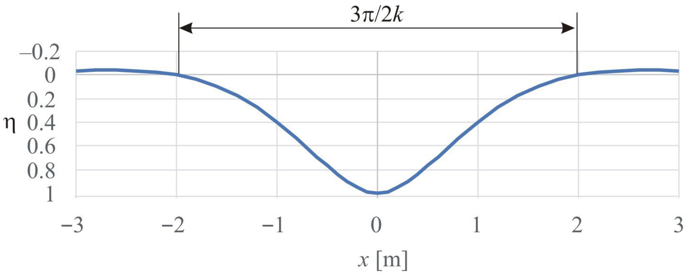
Figure 1. Outline of rail deflection represented by the function η .
Applmech 06 00072 g001
Figure 2. Dependence of the calculated rail deflection length on the deformation modulus of the sub-rail foundation.
Applmech 06 00072 g002
Figure 3. Analytical scheme of load transfer between railway track elements; figure based on [35].
Applmech 06 00072 g003
Figure 4. Stress distribution from three sleepers.
Applmech 06 00072 g004
Figure 5. Options for implementing load transfer from the rail to the sleeper in a mathematical model: (a) the rail bends under the external load, and the deflection profile and amplitude determine the contact forces from the rail to the sleepers; (b) the rail is represented by notional short segments, with the pressure on each sleeper specified separately (for example, based on Equation (5)); (c) the rail transmits the load to the central sleeper only, neglecting the load on adjacent sleepers.
Applmech 06 00072 g005
Figure 6. Computational surface in the adopted coordinate system.
Applmech 06 00072 g006
Figure 7. Computational elementary area (ring).
Applmech 06 00072 g007
Figure 8. Three-dimensional finite element model of a railway track segment (FEM).
Applmech 06 00072 g008
Figure 9. Computational elementary area for a bounded domain.
Applmech 06 00072 g009
Figure 10. Railway track assembly on a conditionally infinite subgrade for the wave propagation model: (a) track length in the model—9.0 m; (b) track length in the model—0.2 m.
Applmech 06 00072 g010
Figure 11. Variation in vertical stresses with depth from the sleeper base along the rail axis.
Applmech 06 00072 g011
Figure 12. Variation of vertical stresses with depth from the sleeper base along the rail axis (single-sleeper configurations).
Applmech 06 00072 g012
Figure 13. Increase coefficient of vertical stresses for models of different lengths.
Applmech 06 00072 g013
Figure 14. Variation in vertical stresses with depth from the sleeper base along the rail axis (multi-sleeper configurations).
Applmech 06 00072 g014
Figure 15. Variation in vertical deflections with depth from the sleeper base along the rail axis.
Applmech 06 00072 g015
Figure 16. Finite element models: (a) length 7.2 m; (b) length 12.0 m.
Applmech 06 00072 g016
Figure 17. Isolines and isofields of vertical deformations in finite element models of different lengths: (a) 0.2 m; (b) 7.2 m; (c) 12.0 m.
Applmech 06 00072 g017
Table 1. Main characteristics of the railway track structure used in the calculations.
Element (Layer)Thickness, mElastic Modulus, MPaUnit Weight, kN/m3Poisson’s Ratio
Rail0.1722.1·10577.00.3
Sleeper0.193 under rail3.6·10424.50.2
Ballast0.510020.00.2
Subgrade4.03518.50.3
Foundation 3018.00.3
Disclaimer/Publisher’s Note: The statements, opinions and data contained in all publications are solely those of the individual author(s) and contributor(s) and not of MDPI and/or the editor(s). MDPI and/or the editor(s) disclaim responsibility for any injury to people or property resulting from any ideas, methods, instructions or products referred to in the content.