Deep Neural Network-Driven Analysis of Free Vibrations in Tapered Beams

Abstract

Most physical systems exhibit nonlinear behavior while in motion, making their resolution challenging due to nonlinearity, dynamic effects, and sensitivity to parameters such as frequency and amplitude. Traditional analytical and numerical approaches can address these challenges but offer high computational costs, particularly in solving the system of free vibrations produced by the tapered beam. Predicting the behavior of this model is complicated, due to its high sensitivity and nonlinearity. Previously, standard neural network models have been used to solve dynamical systems, but they lack efficiency in handling nonlinearity. In this paper, we propose a novel deep learning model that predicts the amplitude of vibrations of a tapered beam. The primary focus of this study is to address the nonlinearity of the model and accurately predict the amplitude of vibrations. To solve this issue, we introduce a deep neural network designed to manage both nonlinearity and dynamical effects, including amplitude. The approach is significant in terms of computational and time efficiency compared to traditional numerical methods. The proposed work provides comparative results generated by the deep neural network, the backward difference formula as an analytical technique, and the Adams–Bashforth–Moulton predictor–corrector method as a numerical approach. The results demonstrate that our model outperforms existing numerical and analytical techniques. With the help of mean square error, Thiel’s inequality coefficient, and mean absolute error, the accuracy of our model can be verified; the lower these values, the more accurate our model will be. In our proposed model, the values are $8.389\times {10}^{-9}$ for mean square error, $5.563\times {10}^{-4}$ for Thiel’s inequality coefficient, and 0.347 for mean absolute error; all these values are close to zero, signifying the accuracy of our model. The conclusion confirms that our proposed approach, even with changeable hyperparameters, is more suitable and accurate than numerical and analytical methods.

1. Introduction

Dynamical systems are the study of the long-term behavior of evolving systems. The modern theory of dynamical systems [1] originated at the end of the 19th century with fundamental questions concerning the stability and evolution of the solar system. Nonlinearity in physical phenomena is a key component in most of the dynamical systems. These nonlinear models [2] are challenging to solve using conventional methods, as nonlinearity arises mainly due to the complex interactions between variables, dependence on higher-order terms, sensitivity to initial conditions, energy transfer, and dissipation [3,4]. So, to study physical phenomena like robotics [5], material sciences, and biological systems, the study of nonlinearity is of great importance. These nonlinearities are hard to solve by traditional methods because of the time management and complex structures, so we have designed a deep neural network (DNN), which performs effectively and is more suitable for oscillatory problems.

Differential equations are utilized to model nonlinearities inherent in tapered beam models, and nonlinear oscillatory differential equations [6] have gained attention. To deal with these problems, many analytical and numerical approaches have been investigated and discussed in the literature. The most useful methods for solving nonlinear equations are perturbation methods [7,8]. They are not valid for strongly nonlinear equations and have many shortcomings. To overcome these shortcomings, new techniques have appeared in the open literature such as variational iteration techniques [9,10,11,12], parameter expansion [13,14], and energy balance [15]. This study uses a novel neural network-based method to solve the free vibrations in tapered beams. The model is nonlinear and it is presented in [16]. Neural networks are created for the purpose of solving differential equations through grammatical evolution, which is the development of network topology by training the network’s parameters with the aid of standard algorithms [17].

Artificial Intelligence (AI) is the simulation of human intelligence processed by machines. In AI, scientists model machines that can think like human brains and process very effectively [18]. Neural networks (NNs) are used to deal with complex systems including real-world nonlinear phenomena [19] such as object detection [20], dynamical systems [21], biophysics [22], health awareness interventions [23], and image classification [24]. DNNs [25] emerge as efficient tools for nonlinear problems in system identification as they can analyze data and learn it without the need to explicitly model the system’s complexities and nonlinearities in any way [26].

Recently, in a variety of engineering tasks, the effective design, analysis, and structural integrity have required dynamic response prediction through linear and nonlinear vibration analysis. In composite structures and environmental disturbers, long-term vibrations [27], which require cyclical or periodic motion constituents to rise, are extremely relevant (and sometimes lead) to unpredictable dynamic behavior, which can lead to catastrophic failure. Recently, nonlinear vibrations of nano and micro [28] structures have been considered as a basic resonance.

Tapered beam vibrations have been widely analyzed using analytical, numerical, and experimental techniques. The traditional methods of Rayleigh–Ritz and Galerkin have been comprehensively employed in approximating the natural frequencies and mode shapes, while Finite Element Methods [29,30] (FEMs) have presented high accuracy when dealing with complexities in geometry and boundary conditions but at a major computational cost. Regardless of the progress made in these areas, a number of research gaps remain to be exploited. These methods are unable to predict the behavior of the underlying system when the parameters used in the dynamics are changed, whereas deep networks understand these complex patterns. Furthermore, the effects of network structure, hyperparameter choice, and training approach on model performance are yet to be explored. Closing these gaps through the application of deep learning methods has the potential to result in more effective and precise predictive models for the analysis of free vibrations in tapered beams, providing a computationally feasible alternative to existing methodologies.

However, DNNs can fit nonlinear mappings quite well, to the extent of only requiring physics-based models to perform. Classical approaches fail to capture the complex behavior of tapered beams, especially for non-uniform shapes and non-constant boundary conditions. Recently, DNNs have gained significant attention as an effective method to solve differential equations and represent dynamic systems, and physics-informed neural networks (PINNs) and fully connected neural networks (FCNNs) are found to have potential in vibration analysis. Yet, their extension to tapered beams is in its infancy, with few studies fully comparing DNN-based approaches with analytical and numerical solutions.

The problem of the nonlinear free vibrations of tapered beams involves a governing Ordinary Differential Equation (ODE) with explicit solutions which can be computed numerically and utilized as training data. Hence, in our case, it was possible to take advantage of supervised training with known solutions instead of embedding the physics in the loss function as in PINNs.

PINNs are more effective in solving systems that do not have explicit solutions but only the conditions and fewer training datasets. In our case, the ability to generate abundant synthetic data using LSODA and BDF made this a straightforward problem, and thus using a purely data-driven FCNN proved to be more efficient in terms of computation.

AI methodologies [1], through training on experimental or simulating data, may therefore be useful in providing solutions to complex systems at lower computation costs while enhancing the potential for scalability across a range of problem areas. For solving differential equations, a user-friendly program is highly beneficial, enlisting the help of a programming language like Python 3 [31], which is highly useful in machine learning [32,33,34] and deep learning [35] tasks.

Tapered beam free vibration [36] prediction and analysis, accurate to a high degree, has far-reaching applications in many fields of engineering and science. Structural engineering exploits these approaches to make stable and efficient bridges, aircraft wings, and skyscrapers by optimizing the use of materials and reducing vibration-induced failures. Aerospace engineering utilizes rigorous vibration modeling to make aerospace components more durable and efficient. In robotics and biomechanics [37], in fact, an insight into nonlinear dynamic behavior plays a fundamental role in developing soft robotic arms and prosthetics. By making effective use of deep learning to offer enhanced precision with reduced computation needs, the proposed research here opens up an elegant solution to facilitating these applications for real-world deployments, an advantage over classical numerical and analytical means.

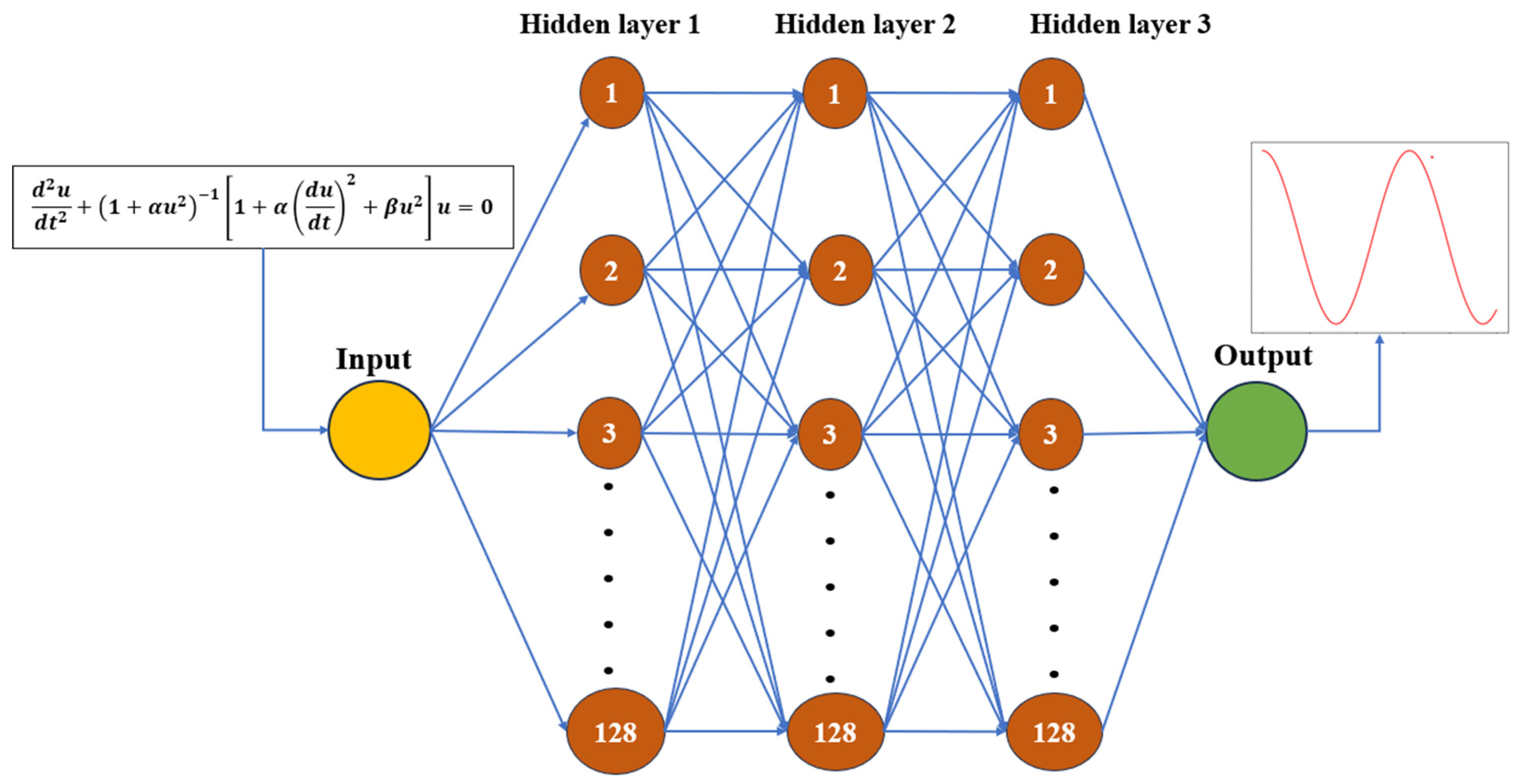
The rest of the paper discusses the nonlinear problem of the tapered beam being modeled [16] and the results generated with the help of a deep learning model. A fully connected neural network (FCNN) [38] consists of an input layer, three hidden layers with 128 neurons in each, and an output layer [39]. The sine activation function (SinActv) [40] is used to capture the periodic behaviors. It is a typical trigonometric function [41] that applies a sine to its input values. For the best optimization and training of our DNN, the Adam [42] optimizer is an appropriate choice [43]. For the model to be able to represent a variety of system behaviors, a synthetic dataset was created by numerically solving the governing differential equation with various initial parameters. We demonstrate the DNN model’s repeatability, stability, and dependability which is supported by these low error values. This study increases practical relevance and reproducibility for future work, which is achieved by combining in-depth statistical analysis [28] with effective computation. The FCNN is designed in such a way that it generates parameters like weights and biases and tunes them with the help of optimizer to obtain the best results.

In Section 2, the mathematical formulation of our problem is discussed, and in Section 3, a methodology to solve the mathematical model is proposed along with the experimental setting that includes a discussion of solutions obtained analytically, numerically, and with the help of the DNN. Section 4 presents and discusses in detail the results generated by our model, and, finally, we conclude the paper in Section 5.

2. Mathematical Formulation

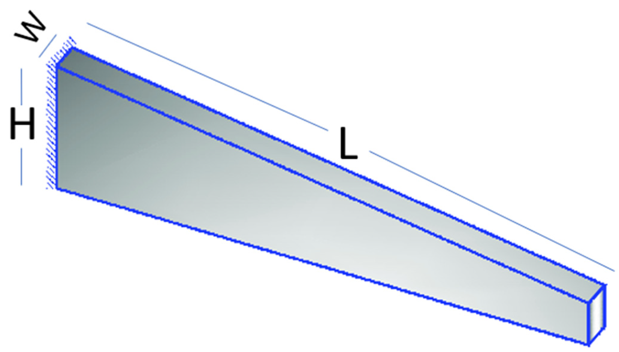
The concern of this paper is mainly the vibrations of tapered beams. In Figure 1, the model shows that the schematic diagram of the tapered beam is a dynamical system [44], which is a structural element that exhibits a variable cross-sectional profile along its length. The deflection of the beam rises with length, but also increases with breadth and height reduction, causing vibrations to occur continuously. The beam may either expand or contract in width or depth, resulting in a gradually changing cross-section. A nonlinear Partial Differential Equation (PDE) that exists in both space and time regulates the nonlinear vibration of beams [16]. The dimensionless governing differential equation is

$${\displaystyle \frac{d^{2}u}{{dt}^2}}+{\left(1+\alpha u^2\right)}^{-1}\left[1+\alpha {\left({\displaystyle \frac{du}{dt}}\right)}^2+\beta u^2\right]u=0$$

(1)

In Equation (1), u is the displacement covered by the beam in vibrational motion, where $\alpha$ and $\beta$ are arbitrary constants that can be assigned any value for the prediction of solutions, and the displacement is dependent upon time t, with the initial condition given as $u\left(0\right)=A$, where A is the highest amplitude and $u^{\prime }\left(0\right)=0$.

Figure 1. Schematic representation of a tapered beam. “H” denotes the height of the beam, “L” is the total length from the fixed point to the movable part, and “W” is the width of the clamped part.

Figure 1. Schematic representation of a tapered beam. “H” denotes the height of the beam, “L” is the total length from the fixed point to the movable part, and “W” is the width of the clamped part.

The change in arbitrary constants and initial conditions gives the change in deflection of the beam at specific time intervals, as the displacement and magnitude of vibrations depend on the initial conditions.

3. Methodology

In our proposed work, a DNN model, shown in Figure 2, is designed in such a way that it can find the solution of tapered beam vibrations (1). The task is to train the network so that it can predict the solution of a nonlinear dynamical system in an efficient and reliable way. The first task is data preparation; then, the network is configurated and the training process is performed.

3.1. Data Preparation

In order to train the FCNN, a comprehensive dataset (X, Y) is generated during the training process with the help of initial conditions (ICs) depending upon the independent variable time. For different BCs, the amplitude of the vibrational motion is different, so in order to train the network, changes in these conditions help in the training process. The dataset was created synthetically by solving the governing differential Equation (1) across a time interval of $[0,T]$ with a time increment of $\mathsf{\Delta }t=0.01$. This produces $N=1000$ time points for each simulation. By changing the parameters $\alpha , \beta$, and initial amplitude $u\left(0\right)=A$ to the values 0.1, 0.2, and 0.3 for $\alpha$, 0.1 and 0.09 for $\beta$, and 0.1, 0.4, and 1 for A, the data is uniformly sampled. This gave a total dataset. No artificial noise was introduced as the intention of this study was to validate the method with clean data before advancing to experimental data with noise.

3.2. Network Configuration

We initialize our model with an FCNN which has one input layer, one output layer, and three hidden layers; each layer is connected with weights and biases. The result from each neuron is multiplied by the weights [45] and combined with the bias term given by the formulation (2), where $x$ is the input, $w_i$ is the weight, $b_i$ is the bias term, and $z_i$ is the result from the respective neuron on which the activation function [46] is applied to stimulate the result, which then acts as the input for the next neuron.

$$z_i=\sum _{i=1}^n{w}_i\ast x+b_i$$

(2)

The activation function (3) is a change in activating neurons, used to create nonlinearity between the levels.

$$I\left(z_i\right)=Sine\left(z_i\right)$$

(3)

The activation function used in our setup, the sine activation function [47], is oscillatory and non-monotonic. This type of function (3) is used to model the periodic behavior of the vibration. This characteristic of the sine activation function enhances the ability of our network to predict the oscillations of our model. Discussing the role of the activation function, a specific threshold is used to activate the function so that the neuron is stimulated, and this process continues until the output layer is reached.

3.3. Training Procedure

In this baseline architecture of our DNN, we adjusted the hyperparameters with the help of the Adam optimizer that clamps the hyperparameter values through practical steps of combining optimization with momentums (4) and modifying the learning rates, which guarantees smooth and efficient training [48]. It maintains an exponential change in average of past gradients $\left(g_t\right)$ to help in smoothing out the changes in parameters during learning.

$$m_t={\beta }_1{m}_{t-1}+\left(1-{\beta }_1\right)g_t$$

(4)

At the same time, it keeps track of an exponential moving average of squared gradients (5) to scale learning rate adaptability with momentum ${\beta }_1$ and scaling term ${\beta }_2$.

$$u_t={\beta }_2{u}_{t-1}+\left(1-{\beta }_2\right)g_t^2$$

(5)

The bias in the estimates, particularly in the first few iterations, is corrected to ensure accuracy. The first and second momentum, here denoted as $m_t$ and $u_t$, are updated by the following technique (6). ADAM then applies model updates based on moment estimates obtained by scaling using the root of the second moment.

$$m_t^{\prime }={\displaystyle \frac{m_t}{1-{\beta }_1^t}} \& u_t^{\prime }={\displaystyle \frac{u_t}{1-{\beta }_2^t}}$$

(6)

This division guarantees that within each moment, the learning rates are reasonable for each parameter. ADAM updates the weights ${\theta }_t$ by corrected moment estimate and small learning rate $\alpha$ by using (7), and to avoid zero division, a small value parameter $ϵ$ is used; these values are generated after each iteration and are not the fixed values: as the process repeats itself, the values change and the other hyperparameters like the learning rate are modified with the optimizer.

$${\theta }_t={\theta }_{t-1}+{\displaystyle \frac{\alpha m_t^{\prime }}{\sqrt{u_t^{\prime }}+ϵ}}$$

(7)

ADAM adjusts the values to help in gradually modifying the state of the neural network while avoiding vanishing or exploding gradients; the level of error mitigation when compared to other optimizers is much higher, making it extremely productive when used in deep learning scenarios.

Table 1. Description of the DNN architecture which generates the best results.

Sr. No.	Parameters	No. of Parameters	Best
1	Neurons in each hidden layer	(128, 128, 128)	128
2	Activation function	Sine activation, ReLU, tanh, sigmoid	Sine
3	Epochs	3000, 10,000, 30,000	30,000
4	Learning rate	0.001, 0.01	0.001

shows information on the parameters of our neural network which generates optimized and accurate outcomes.

The loss is calculated with the help of mean squared error (MSE) [49], mean absolute error (MAE), and Thiel’s inequality coefficient (TIC). For MSE, the Formula (8) is used to calculate the average of difference between the actual values obtained analytically and the output values predicted by the DNN to measure the performance of the model during training.

$$MSE={\displaystyle \frac{1}{N}}\sum _{i=1}^N{\left({y_i}_{true}-{y_i}_{predicted}\right)}^2$$

(8)

Another technique to calculate the efficiency of the model is by TIC [50], which is commonly used for inequality measurements as it satisfies important axiomatic requirements such as the principle of transfer and decomposability.

$$TIC={\displaystyle \frac{\sqrt{\frac{1}{N}{\sum }_{i=1}^N{\left(A_i-P_i\right)}^2}}{\sqrt{\frac{1}{N}{\sum }_{i=1}^N{A}_i^2+\sqrt{\frac{1}{N}{\sum }_{i=1}^N{P}_i^2}}}}$$

(9)

In (9), $A_i$ is the actual value and $P_i$ is the predicted value. This provides a measure of how well a model works; the closer the value to zero, the better the model’s performance.

For measuring the accuracy of the DNN, MAE can also be implemented, which is the measure of average absolute difference between the actual $A_i$ and the predicted value $P_i$ (10). With MAE, we can actually evaluate the overall predictive accuracy of a DNN and optimize it for improved accuracy and generalization.

$$MAE={\displaystyle \frac{1}{n}}\sum _{i=1}^n|A_i-p_i|$$

(10)

The training of the DNN model for approximating the solution of a dynamical system is performed in an efficient way with the help of MSE, TIC, and MAE.

The numerical solution is obtained by the Adams–Bashforth–Moulton predictor–corrector method, indicated as (LSODA), which refines the prediction [51] using the derivative at different step sizes. In particular, using the Adams–Bashforth component as a predictor, the next value of the solution is extrapolated in linear form based on previously taken steps. When the predictor provides the solution, the Adams-Moulton component works as the corrector by adjusting the estimate with the aid of a current derivative. This corrector step is implicit and improves the stability of the algorithm, notably in the case of stiff equations [52]. The predictor and the corrector act in a harmonious balance, assuring accuracy in the solution and the efficiency of computations, making LSODA an effective method for solving ODEs.

For analytical solutions, the backward difference formula [53] is used, which is mostly useful for solving dynamical systems such as tapered beams. This method calculates the current solution by taking a linear combination of past solutions with a time derivative. Every time step needs to be solved by forming the Jacobian matrix while solving nonlinear problems [22]. Since this would be more costly in computation as compared to our DNN model, an FCNN is employed to solve the ODE. This approach is based on the neurodiffeq package, which uses automatic differentiation and custom architectures for solving differential equations.

3.4. Experimental Settings

In order to implement the FCNN over this model, we employed a Python library called neurodiffeq, which is a famous library for solving differential equations using neural networks [54]. We used different packages from this library and modified those packages according to the complexity and behavior of our model. In this section, we are going to discuss the neurodiffeq library and its packages along with the modifications made to them in detail. The dataset (X, Y), generated during the training process with the help of initial conditions (ICs) across different time intervals, does not have any noise during generation, as the goal was to first validate the model performance on clean data before applying to real-world noisy measurements, as discussed in detail in Section 3.1.

Neurodiffeq is a Python library that is designed to solve differential equations using neural networks. It pulls deep learning models, specifically neural networks, to approximate solutions to ODEs as well as partial differential equations (PDEs) [55]. It formulates solving differential equations as a neural network by considering it an optimization problem. For this purpose, it reformulates the mathematical model as

$$L{S}_i-P=0$$

(11)

In Equation (11), L is the differential operator, $S_i$ is the solution which needs to be approximated, and P are the rest of the terms.

The differential equation is represented in the form of a loss function, and then the neural network learns to minimize this loss function with the help of squared loss, as shown in Equation (12).

$$loss={\left(L{S}_i-P\right)}^2$$

(12)

In this research, the squared loss function is used to estimate the accuracy of the DNN in approximating the vibration response of the tapered beam. The squared loss in our case is MSE (8), which, when the average is taken over several data points, is the sum of the squared difference between the predicted and the reference or exact values. In solving the differential equation, the squared loss function assists in reducing the residual between the predicted displacement and the true solution to enhance the precision of the neural network. In the training process, the DNN modifies its weights and biases to reduce this loss, and it converges to zero values. Through the utilization of this loss function, this work guarantees that the DNN will learn to approximate the solution with high accuracy.

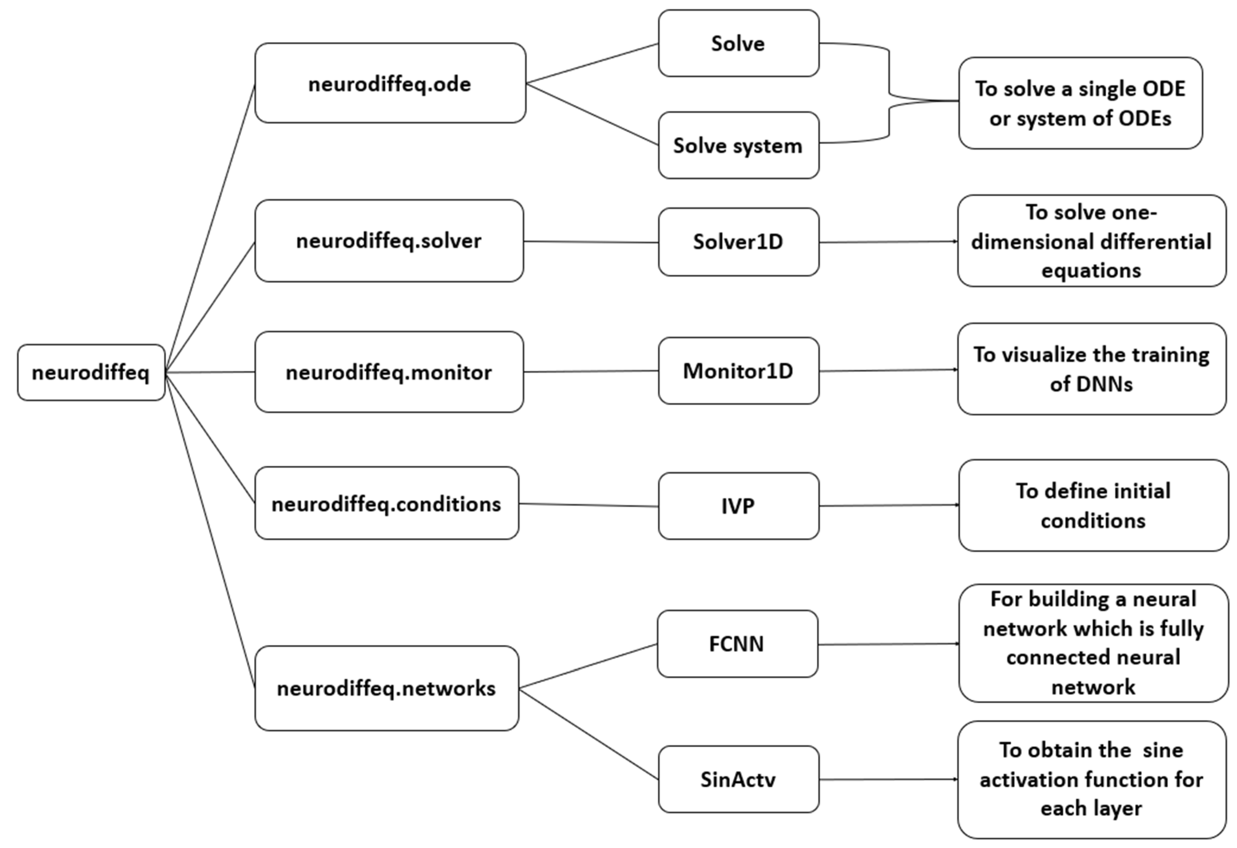
The key features of the library are given [56] with the help of a flow chart in Appendix A, indicating the use of each submodule. In our FCNN architecture, we used the packages “solve” and “solve_system”, which are used to approximate the solutions of differential equations. Another package for solving differential equations being used by FCNNs is “Solver1D”, which is specifically used for simpler, one-dimensional problems, allowing the FCNN model to focus on specific one-dimensional differential equations with efficiency and simplicity in setup. The “Monitor1D” package from neurodiffeq is a tool which helps in the visualization of the training progress of the neural network solution, tracking metrics like the loss and the neural network’s output over training epochs. This is essential for monitoring and debugging the model’s performance, and helps to understand how well the FCNN is approximating the solution. For the assignment of boundary values, a package called “IVP” is imported from “neurodiffeq. conditions” and used for solving initial value problems, as it provides the necessary conditions for the neural network to learn and approximate the solution accurately. Our model uses the “sine activation function”, which is also imported from the neurodiffeq library. The details can be seen in Appendix A.

4. Results and Discussion

This section discusses the results generated with the help of our proposed model in comparison with analytical solutions and numerical techniques. We carried out various experiments to observe how changes in parameter values of nonlinear dynamical systems i.e., $\alpha ,\beta ,A$ provided in Equation (1), and initial conditions can affect the solutions of differential equations as shown in Figure 3a, Figure 4a and Figure 5a.

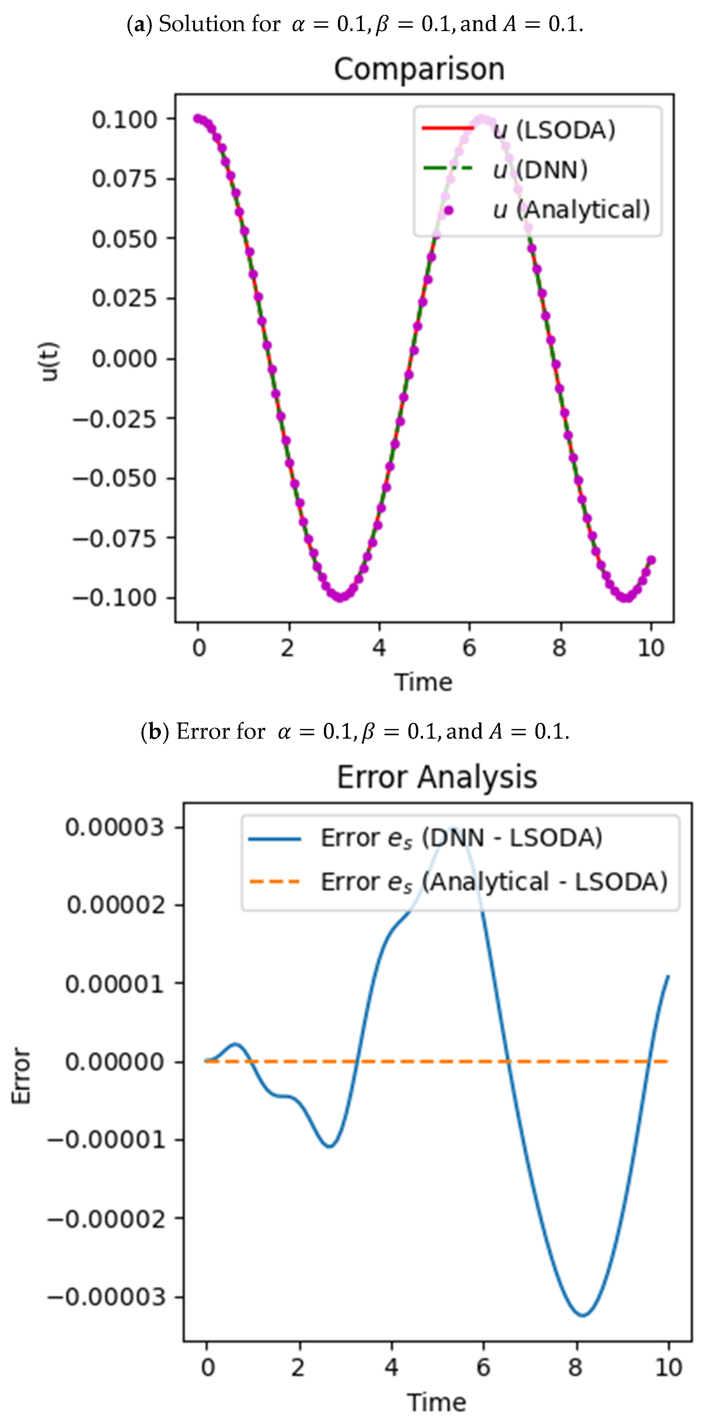
In Figure 3, the results are shown and discussed when the values are $\alpha =0.1$ and $\beta =0.1$, and the initial condition or amplitude is set to $A=0.1$

In Figure 3, we exhibit the accurate displacement of the values of parameters set to $A=0.1,\alpha =0.1,$ and $\beta =0.1$ from the analytical solution generated by BDF (shown by purple dots), the numerical solution by LSODA (shown by red solid line), and that by the DNN (shown by green dashed line) given by Figure 3a. The error shown in Figure 3b between the numerical and the analytical solution is zero, which shows that the values at each interval of time coincide, and for the DNN error, the values remain close to zero, which highlights that while the DNN introduces much less variation, its error remains small, and the analytical solution aligns more closely with the LSODA reference. For the DNN, the curve oscillates slightly but is very close to the expected solution, demonstrating the model’s capability to identify intricate nonlinear behavior. This comparison describes the relative accuracy of the two methods against the numerical solution. The loss during training for the respective values of $\alpha$ and $\beta$, which is given in Figure 3c, decreases to nano (${10}^{-9}$) values, which shows that both curves for training loss and validation loss generally follow a downward trend, indicating that the model is learning effectively. The training loss has fluctuations, typical of gradient-based optimization, but steadily declines. The validation loss closely follows the training loss, showing that the model generalizes well and avoids overfitting. At the end, both losses converge, suggesting that the model has reached a good level of performance on the training and validation data.

Below, Figure 4 describes the detailed results at $\alpha =0.2$ and $\beta =0.3$, with the amplitude set as $A=0.4$.

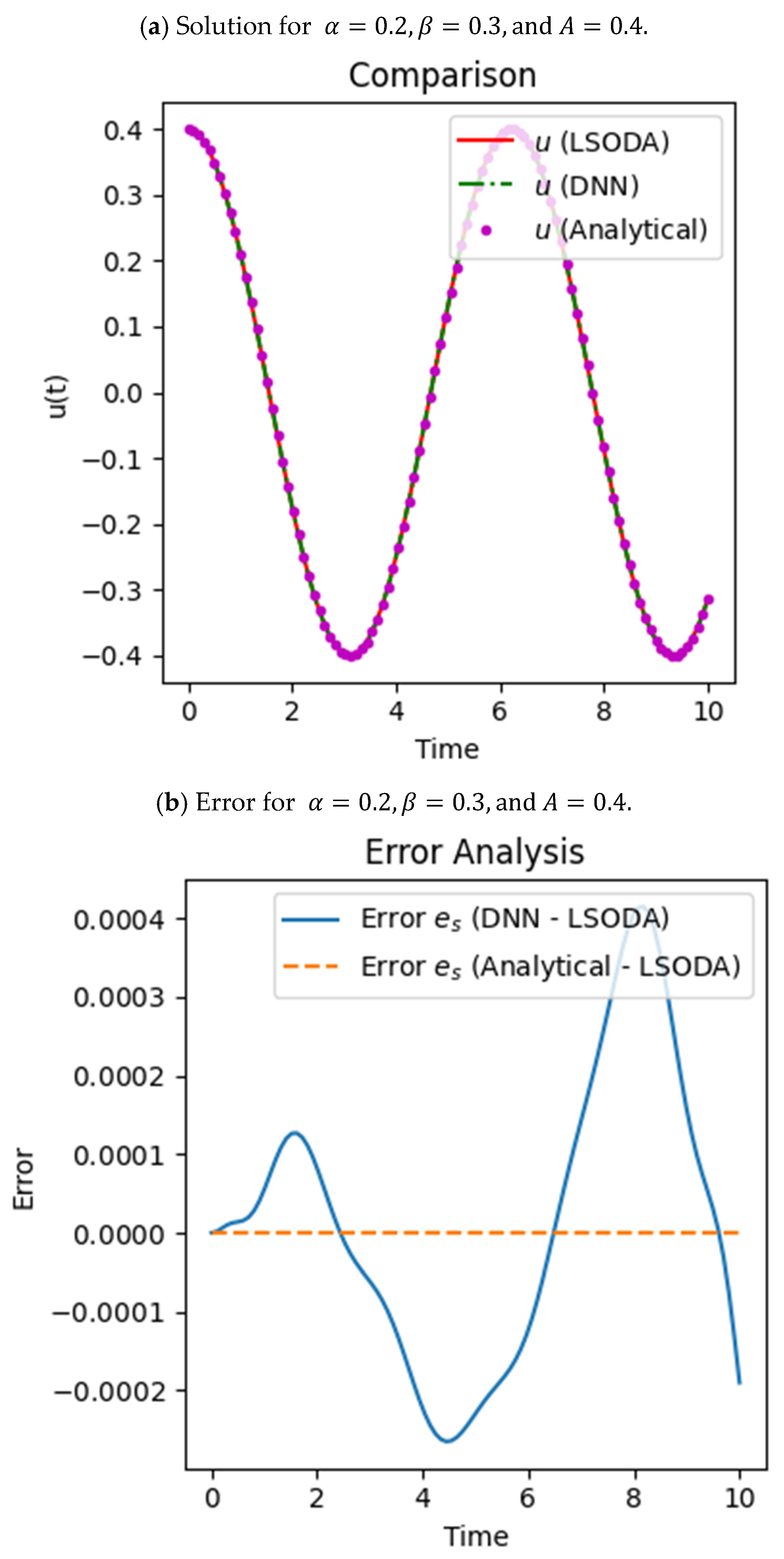
In Figure 4, the graphs are plotted for the displacement value starting from 0.4 in Figure 4a as it depends upon the initial condition $u\left(0\right)=0.4$. 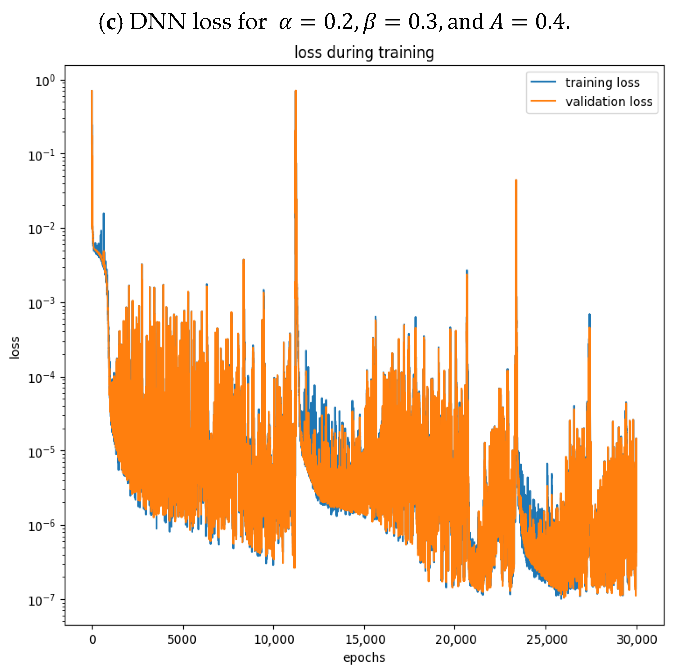It is observed that the displacement obtained from the numerical technique (the Adams–Bashforth–Moulton predictor–corrector method), i.e., LSODA, and the analytical technique (BDF) is the same, which means that the error between these two is zero, which is shown with the help of the error analysis in Figure 4b. The orange dotted line shows that the error is zero, and the blue solid line shows the error between the DNN and the other solution, which is nearly zero. This similarity proves that the trained DNN model gives a precise approximation to the system dynamics. Loss during the training of the model diminishes with epochs, guaranteeing performance improvement over time. In Figure 4c, the training loss and validation loss during training show that over 30,000 epochs, the loss decreases from 1 to ${10}^{-7}$, indicating that the model has trained effectively and can predict the solution to our problem accurately.

In Figure 5, the model is trained by setting the parameters to $\alpha =0.09$, $\beta =0.1,$ and $A=1.0$.

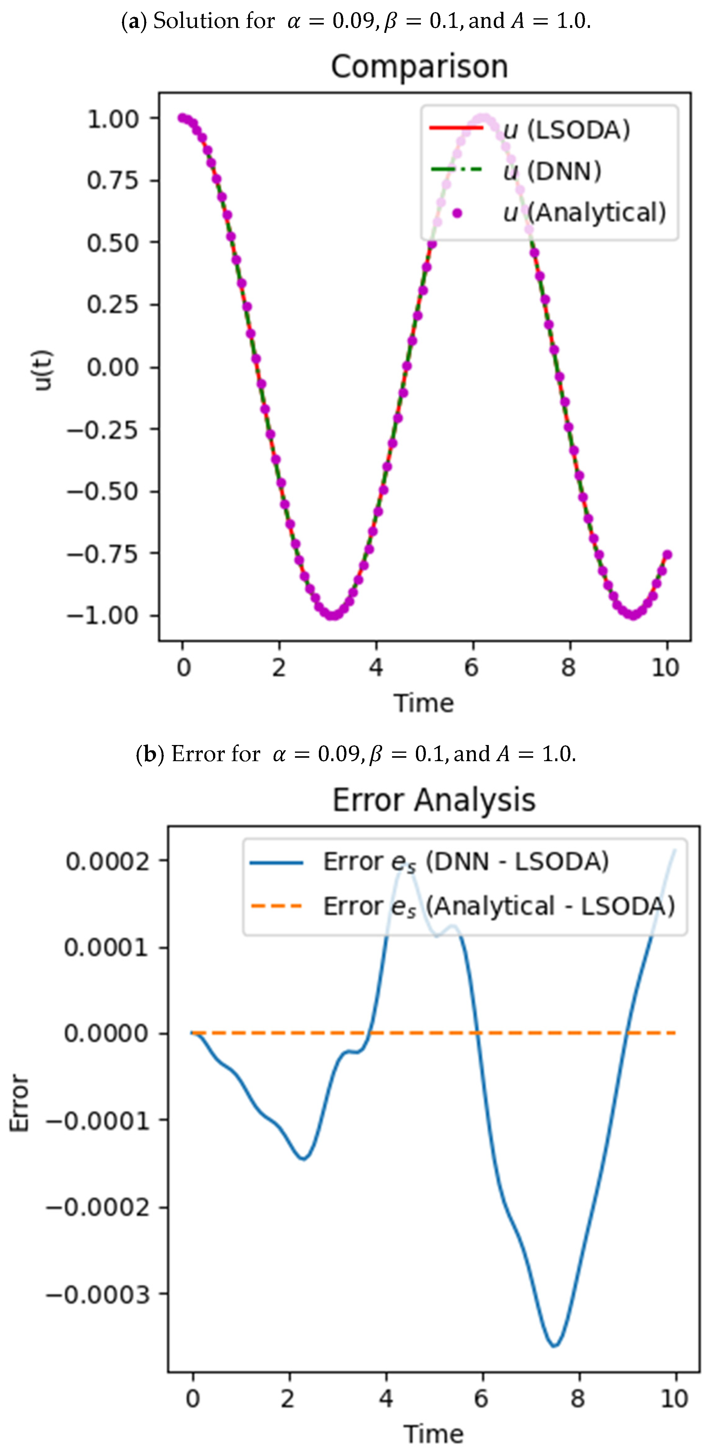
With the help of DNN parameters such as weights and biases, it seems that in Figure 5a, all results coincide with each other and the trained model gives the same results as those obtained numerically and analytically, but a more effective evaluation can be made if one performs the error analysis by calculating and comparing the error graphs between each generating technique and those obtained from our proposed DNN, as shown in 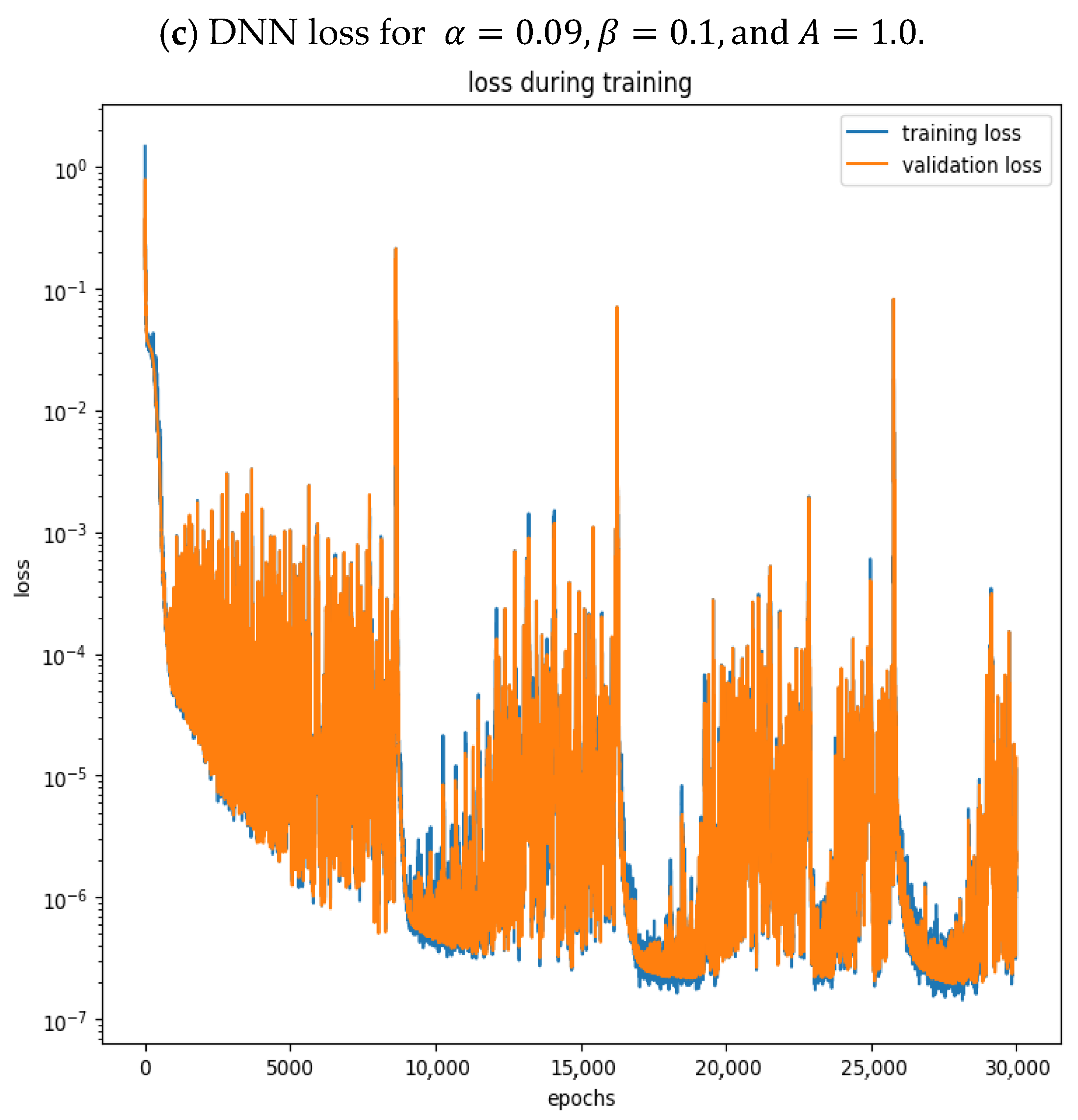Figure 5b. The training and validation losses in Figure 5c converge closely to each other with successive epochs, implying that the model is quite well trained. With the fine-tuning of these parameters, the accuracy of the model increases considerably, where both the reduction in loss and the minimization of error is significantly greater.

With the help of sine activation, the results were obtained for the DNN (Figure 3, Figure 4 and Figure 5), and a comparison with analytical and numerical methods was made along with training and validation loss. The use of oscillatory functions helps in better understanding beam vibrations and predicting the results accurately. On the other hand, if some non-oscillatory function, i.e., ReLU, tanh, and sigmoid, are used, the results get worse.

4.1. Comparison of Sine Activation Function with ReLU

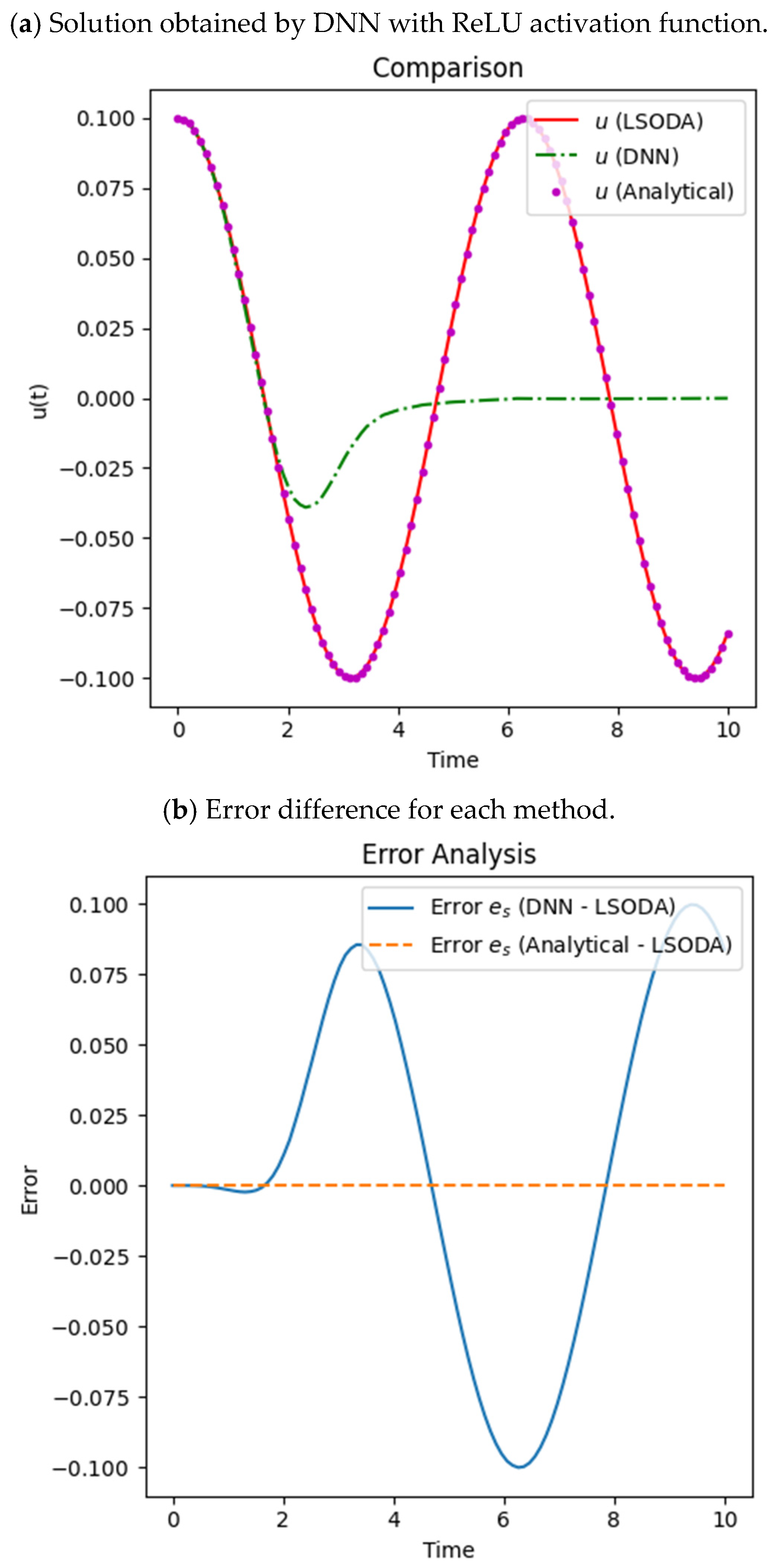
By comparing the results generated by the ReLU activation function, while keeping all the other hyperparameters the same in Figure 6, it can be seen from the error analysis (Figure 6b) and the solution curve (Figure 6a) that the DNN does not give accurate results, so we claim that the use of the ReLU activation function [57] while training the DNN resulted in insufficient performance regarding the solution of the tapered beam problem.

From the comparison plots shown earlier, it is clear that the DNN output is far greater than both the numerical and analytical results, especially after the initial time intervals where periodic behavior is expected, hence failing to capture it accurately. Furthermore, the error analysis (Figure 6b) supports this claim, where large differences are shown for the DNN results against LSODA, with the analytical solution showing close alignment. This lack of good performance is most likely due to the ReLU function being piecewise linear and thus imposing a lack of smoothness and continuity on the network for certain types of oscillatory or sinusoidal problems. Thus, for such problems, ReLU is not an optimal choice, unlike smoother alternatives like sine which would lead to improved performance, as explained in [22,25,45].

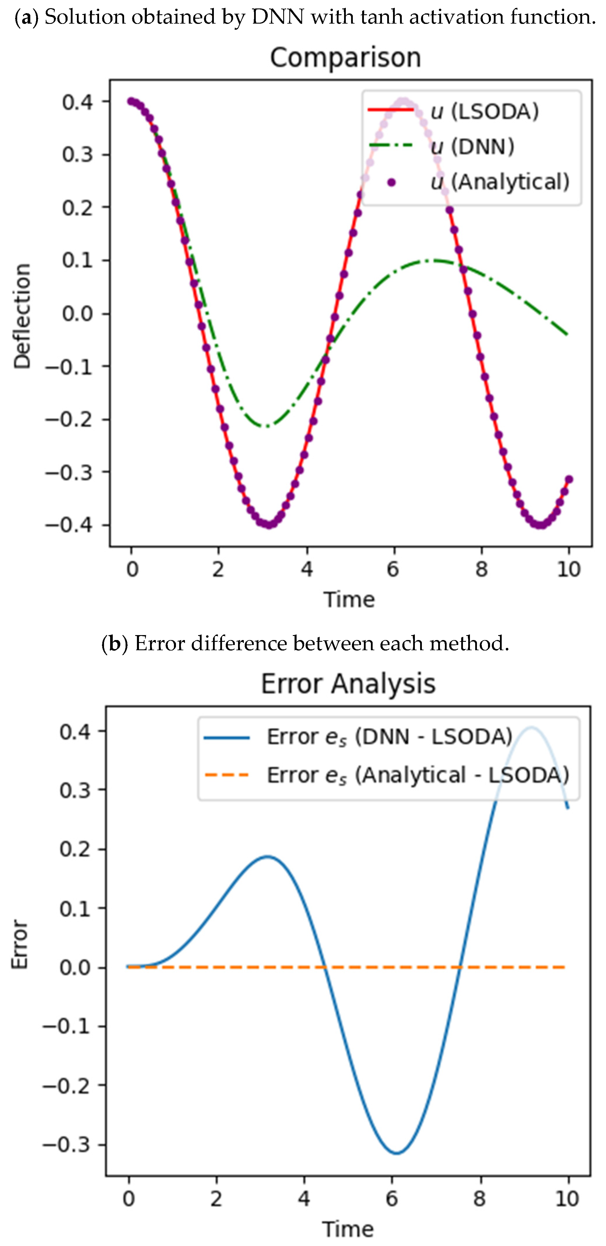
4.2. Comparison of Sine Activation Function with Tanh

The training of the DNN with the help of the tanh activation function is not accurate as it does not match with the numerical solution curve and the reference curve obtained by LSODA (Figure 7a); similarly, the error analysis (Figure 7b) shows that the highest error is obtained between the DNN and the reference curve.

From the comparison plots shown earlier, it is clear that the DNN output deviates from both the numerical and analytical results, especially after the initial time intervals where periodic behavior is expected, hence failing to capture it accurately. Furthermore, error analysis (Figure 7b) supports this claim, where large differences are shown for DNN results against LSODA, with the analytical solution showing close alignment. The DNN struggles with capturing appropriate dynamics, particularly with respect to the magnitude as well as the oscillatory phase, even when trained with tanh, which is a smooth and bounded activation function. This discrepancy results in a large prediction error (Figure 7b) in the deflection curve, indicating that the attempt to train the network with tanh in this case was not successful. These outcomes reinforce the conclusion that in this instance, the use of the tanh function resulted in a failure to converge and produced the worst outcome relative to the other approaches implemented; instead, we may use the sine function to train our model accurately.

4.3. Comparison of Sine Activation Function with Sigmoid Function

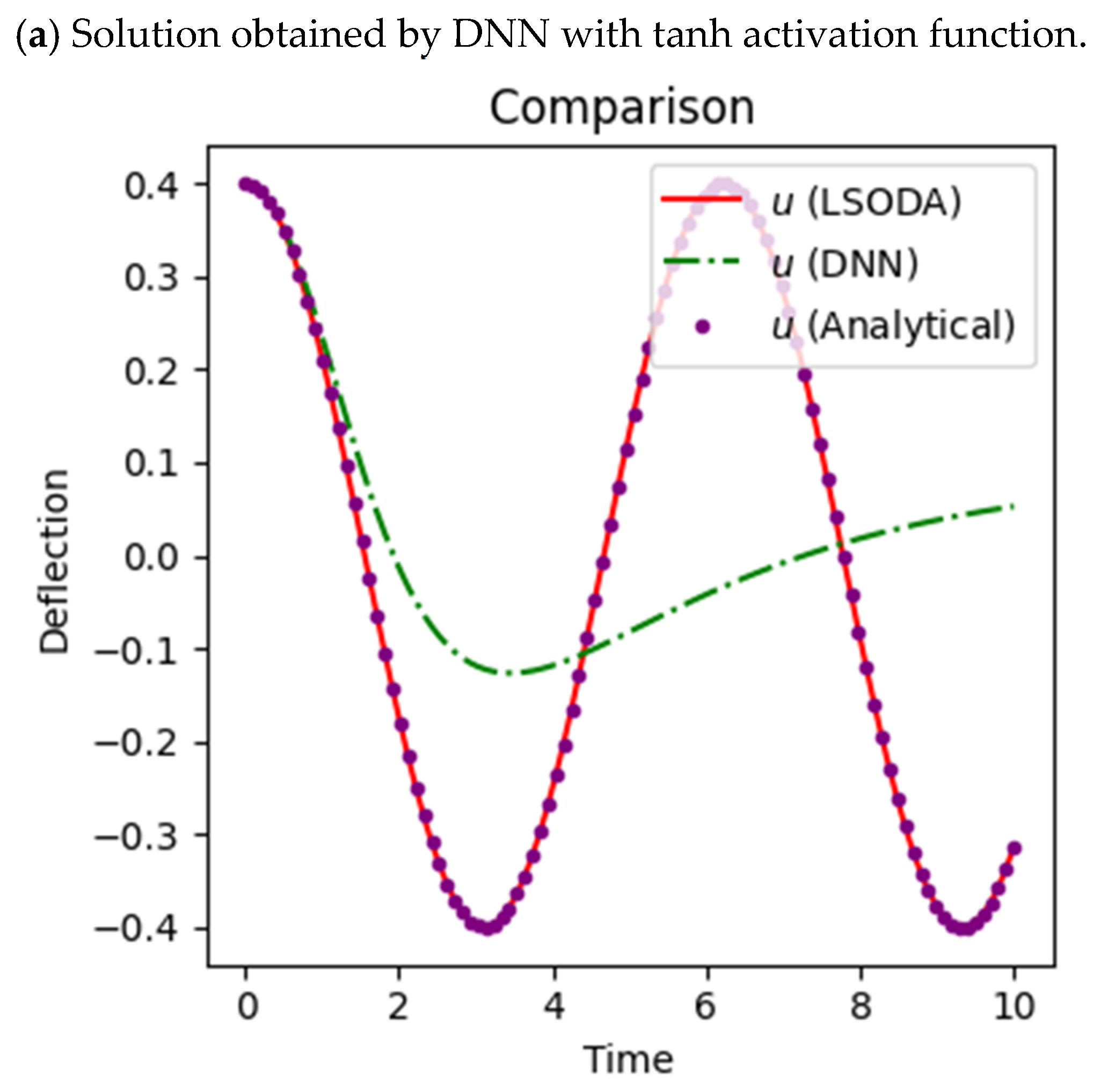
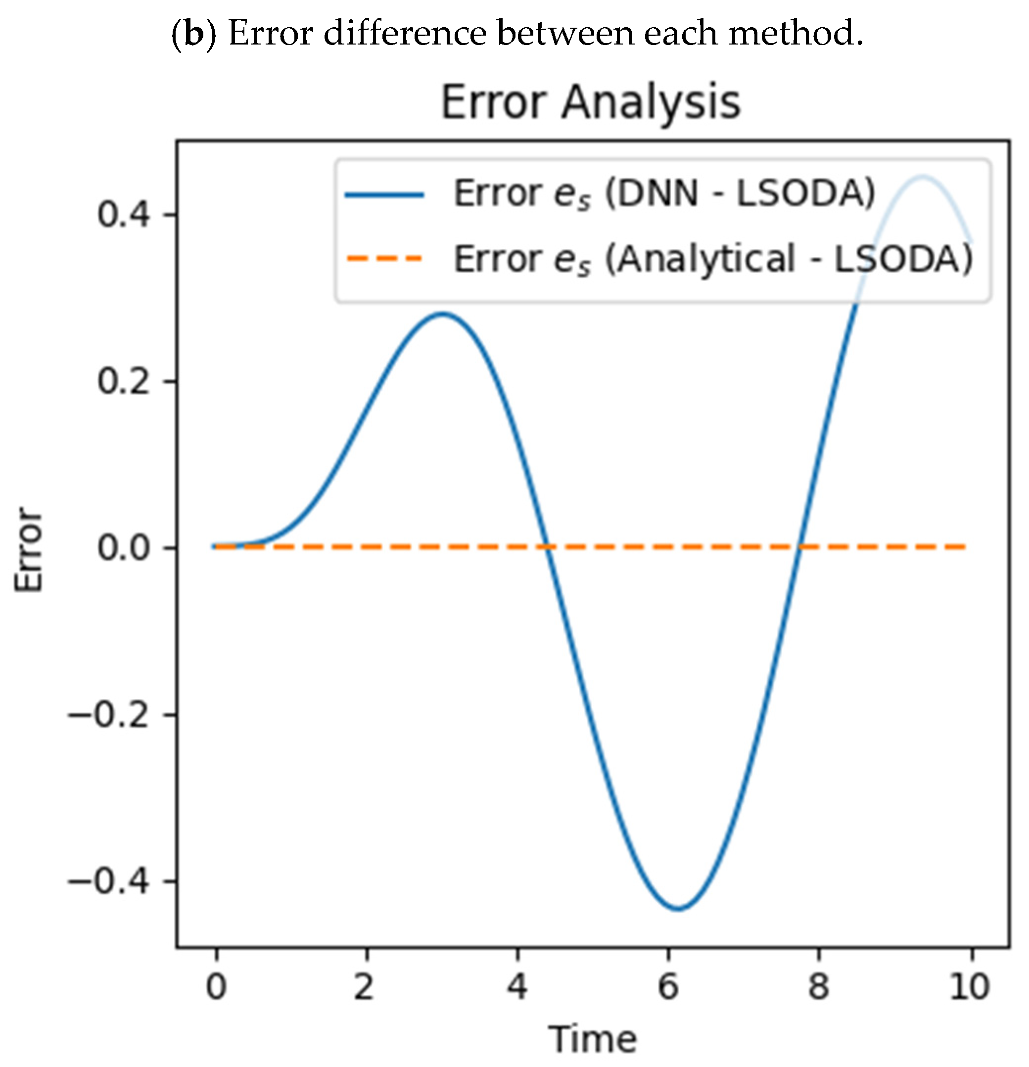
Just like tanh, LSODA and the analytical solutions worked beautifully here and captured the oscillations in the system accurately. But the DNN trained with sigmoid did not capture the correct dynamics (Figure 8a) and deviated greatly in amplitude and phase. This shows that while sigmoid is smooth and popular, it does not train models well for oscillatory problems like this one.

When training the DNN with the sigmoid activation function, it is evident from Figure 8a that the solution curve deviates from the original curves, showing poor accuracy, and this can also be seen in the error graph where the error between DNN and the reference solution (Figure 8b) is very high. It is evident that the more traditional off-the-shelf activations such ReLU, tanh, and sigmoid do not work well to model oscillatory systems. The sine activation function does quite the opposite and relies on the periodicity of the problem, allowing it to work better. The novelty of this work lies in applying sinusoidal activation functions to capture nonlinear periodic vibrations in tapered beams, and its comparison with other non-periodic activation functions given in the above figures shows the true accuracy of the model.

4.4. Statistical Analysis

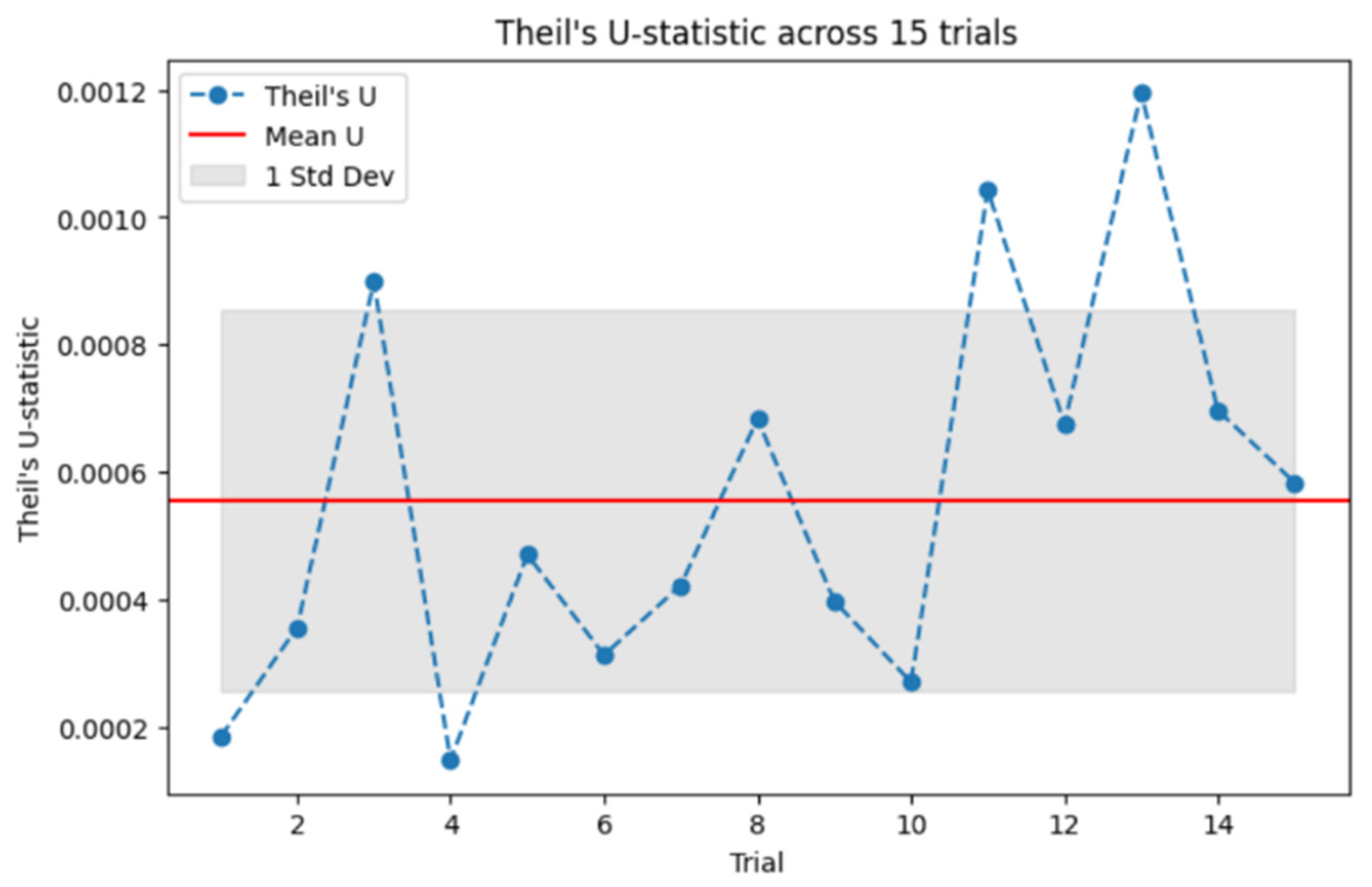
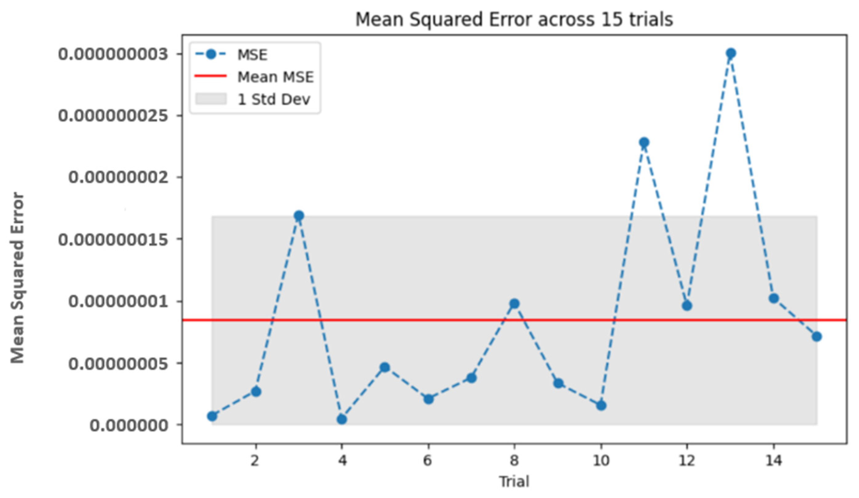
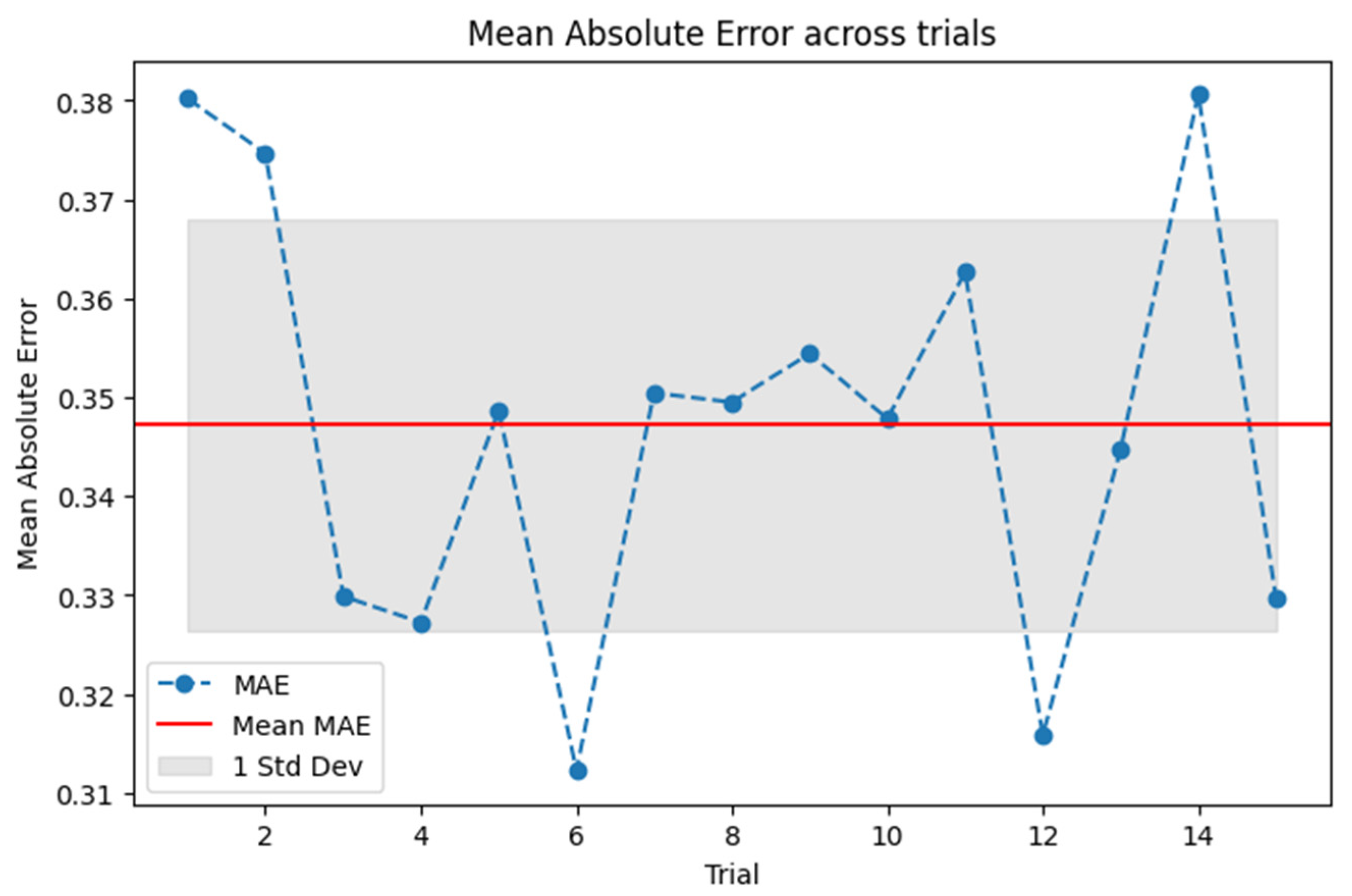
A statistical analysis [58] using 15 trials is conducted to determine the reliability and accuracy of the suggested DNN approach by utilizing TIC and MSE along with MAE. MSE and TIC are calculated through (8, 9), respectively, with the help of actual and predicted values; the analytical approach, i.e., BDF, gives the actual and the DNN generates the predicted values after each trial. Each trial is composed of 3000 epochs, and after each trial, the actual and predicted values are obtained, and TIC and MSE are calculated for all 15 trials in such a manner. After these 15 trials, the average value given by the red line in the figures indicates the average result for both measures. This repeated testing further supports the evidence of the robustness and reliability of the model.

Figure 9 gives the results for TIC; as TIC normalizes the relative error, it is most useful in analyzing the performance of the DNN model with respect to different data points. If the TIC value is very close to 0, then the model successfully describes the inherent dynamics of the vibration of the beam with a negligible prediction error. This excellent agreement between predicted and measured values makes the DNN model a trusted solution for complex nonlinear systems.

A lower MSE value indicates that the model accurately captures the nonlinear vibrational behavior, as smaller squared errors mean less deviation from observed values. Figure 10 shows the MSE between the actual results generated analytically and the predicted results generated by the DNN. This also reflects the model’s robustness in handling the complexities of tapered beam vibrations, a common challenge in nonlinear dynamics.

Figure 11 shows that the MAE value is close to zero, which indicates the accuracy of our DNN model in predicting the amplitude of vibrations. A lower MAE means that the model predicted the values that are closer to the actual values, which represents higher accuracy. MAE is especially favorable when measuring real-world deviations since it disregards all the errors equally without charging more for larger errors than small ones. It is therefore a robust measurement in applications where absolute deviations will be more important and it does not exaggerate gross errors.

Table 2. Statistical analysis of DNN after each trial, calculating TIC, MSE, and MAE.

	Statistical Measure	TIC	MSE	MAE
Trial
After 1st trial		$2\times {10}^{-4}$	$0$	$0.38$
After 2nd trial		$3\times {10}^{-4}$	$2.5\times {10}^{-8}$	$0.375$
After 3rd trial		$9\times {10}^{-4}$	$1.75\times {10}^{-8}$	$0.33$
After 4th trial		$1\times {10}^{-4}$	$0$	$0.326$
After 5th trial		$5\times {10}^{-4}$	$5\times {10}^{-8}$	$0.348$
After 6th trial		$3.8\times {10}^{-4}$	$2.5\times {10}^{-8}$	$0.31$
After 7th trial		$4.1\times {10}^{-4}$	$4\times {10}^{-8}$	$0.35$
After 8th trial		$7\times {10}^{-4}$	$1\times {10}^{-8}$	$0.349$
After 9th trial		$4\times {10}^{-4}$	$4\times {10}^{-8}$	$0.355$
After 10th trial		$3\times {10}^{-4}$	$1\times {10}^{-9}$	$0.347$
After 11th trial		$1\times {10}^{-3}$	$2.25\times {10}^{-8}$	$0.36$
After 12th trial		$7\times {10}^{-4}$	$1\times {10}^{-8}$	$0.315$
After 13th trial		$1.2\times {10}^{-3}$	$3\times {10}^{-9}$	$0.345$
After 14th trial		$7\times {10}^{-4}$	$1\times {10}^{-8}$	$0.38$
After 15th trial		$5.57\times {10}^{-4}$	$3\times {10}^{-8}$	$0.328$

displays the outcomes after each trial for TIC, MSE, and MAE, which demonstrate the insights of the statistical analysis.

In Table 2, the statistical measures TIC, MSE, and MAE are calculated over 15 independent training trials of the proposed model. The outcomes illustrate the low error values across all the trials, proving the model’s validity. The mean TIC value achieved is $5.56\times {10}^{-4}$, given in Figure 9, the mean MSE is $1.95\times {10}^{-8}$, given in Figure 10, and the mean MAE is approximately 0.347, shown in the above Figure 11. Thus, these results reinforce the conclusion that the model effectively and accurately represents the nonlinear response of tapered beams to vibrating loads, consistently achieving a tight fit between the computed and actual results. This analysis increases confidence in the flexibility and consistency of the proposed deep learning framework after multiple trials.

5. Conclusions and Future Work

In conclusion, the proposed deep neural network-based strategy has demonstrated its superiority in solving the complex nonlinear dynamical system of free vibrations in tapered beams. Through a series of experiments, we have shown that our model effectively captures nonlinearity, including parameter variations such as amplitude, surpassing the limitations of traditional numerical and analytical methods. A key novelty of this work is the integration of deep learning techniques to model nonlinearity with higher computational efficiency and accuracy compared to conventional approaches. Our comparative analysis, including error and statistical evaluations, provides critical insights into how well the model identifies deviations, trends, and the impact of parameter variations. The graphical findings further validate the effectiveness of our approach. Furthermore, the statistical analysis, performed with the help of trials for different statistical measures, explains the robustness and accuracy of the proposed method. The low values indicate the stability of our model towards highly nonlinear complex dynamical systems. Unlike traditional methods, which are often computationally expensive or less adaptable to dynamic parameter changes, our model significantly improves efficiency and prediction accuracy. This study highlights the immense potential of deep learning in addressing nonlinear dynamical systems, paving the way for future advancements in this domain. The proposed strategy can also be extended by incorporating advanced activation functions and hybrid learning techniques to further enhance performance and adaptability. Our findings contribute to the ongoing evolution of AI-driven approaches in physics-based modeling, offering a robust foundation for future research in solving complex nonlinear systems. Future research may aim to enrich the suggested model by adding deeper activation functions and hybrid learning methodologies to enhance performance and adaptability. Investigating attention mechanisms or physics-informed constraints may even further enhance precision. Further extension of the technique to multi-dimensional and time-varying systems would make it more versatile. Incorporating methods for uncertainty quantification may even be used to estimate model robustness under diverse conditions.