Article

Impact of Far- and Near-Field Records on the Seismic Fragility of Steel Storage Tanks

by
Giammaria Gabbianelli
1,
Aldo Rapone
2,
Riccardo R. Milanesi
3 and
Roberto Nascimbene
2,*
1
Department of Civil Engineering and Architecture, University of Pavia, 27100 Pavia, Italy
2
Department of Science, Technology and Society, University School for Advanced Studies IUSS Pavia, 27100 Pavia, Italy
3
European Centre for Training and Research in Earthquake Engineering, EUCENTRE, 27100 Pavia, Italy
*
Author to whom correspondence should be addressed.
Appl. Mech. 2025, 6(2), 24; https://doi.org/10.3390/applmech6020024
Submission received: 20 February 2025 / Revised: 24 March 2025 / Accepted: 28 March 2025 / Published: 30 March 2025

Abstract

:
Liquid-storage tanks are critical components in industrial plants, especially during seismic events. Tank failures can cause significant economic losses, operational disruptions, and environmental damage. Therefore, accurate design and performance evaluation are essential to minimize these risks. However, past earthquakes have highlighted the need for a better understanding of tanks’ seismic behavior. This requires selecting the appropriate seismic input and ground motion records to properly simulate tank responses. This study examines the seismic behavior of various tank types using different earthquake record sets, including both far-field and near-field events. The tanks were modelled with varying geometries, such as diameter–height ratios, wall thickness, liquid height, and radius. Time-history analyses were conducted to generate fragility curves and evaluate the seismic performance of the tanks based on specific limit states. The findings show that the choice between far- and near-field records significantly influences seismic response, particularly in terms of fragility curve variation. The fragility curves derived from this analysis can serve as valuable tools for risk assessments by governments and stakeholders, helping to improve the safety and resilience of industrial plants.

1. Introduction

Recent studies and post-earthquake inspections have highlighted the effectiveness of modern building codes in minimizing human casualties during intense seismic events. With life safety essentially ensured, research efforts have shifted towards assessing economic losses, particularly those caused by downtime and damage to nonstructural elements, which are especially critical in industrial facilities [1,2,3].
Steel storage tanks are among the most common structures in industrial plants for liquid storage, playing a vital role in functionality and safety. Following past earthquakes, numerous studies have been conducted to analyze and monitor the behavior of these tanks and their stored liquids [4,5]. Typical damage mechanisms include localized buckling at the base of the tank wall, known as elephant-foot buckling (Figure 1a), fluid sloshing and its associated impacts (Figure 1b), failure or disconnection of attached piping systems (Figure 1c), and vertical uplift or overall structural instability of the tank (Figure 1d). Past studies [2,3,4,5,6,7] have noted that these failures are primarily attributed to the standardized nature of tank fabrication rather than to deficiencies or delays in the development and application of seismic design codes and guidelines. It should be noted that the failure or damage of a tank—whether due to sloshing effects, pipes, buckling, uplift, or instability—can lead to hazardous substance spills, resulting in facility downtime and, in severe cases, catastrophic environmental pollution and human casualties.
To better understand the seismic response of storage tanks, Malhotra [8,9] developed a simplified model that predicts the behavior of cylindrical tanks under seismic loads. This model employs a mechanics-based mass-spring-dashpot analogy to account for impulsive and convective motion components separately.
However, it should be noted that for more insight into the assessment of EFB damages in steel storage tanks, several studies developed refined 3D models [10,11,12,13,14,15,16,17].
This study aims to assess the seismic vulnerability of Italian industrial plants by analyzing a large set of steel tanks using Malhotra’s model, considering both anchored and unanchored configurations. The investigation covers three Italian seismic zones—low, medium, and high seismicity—examining the impact of different ground-structure connection types on tank performance.

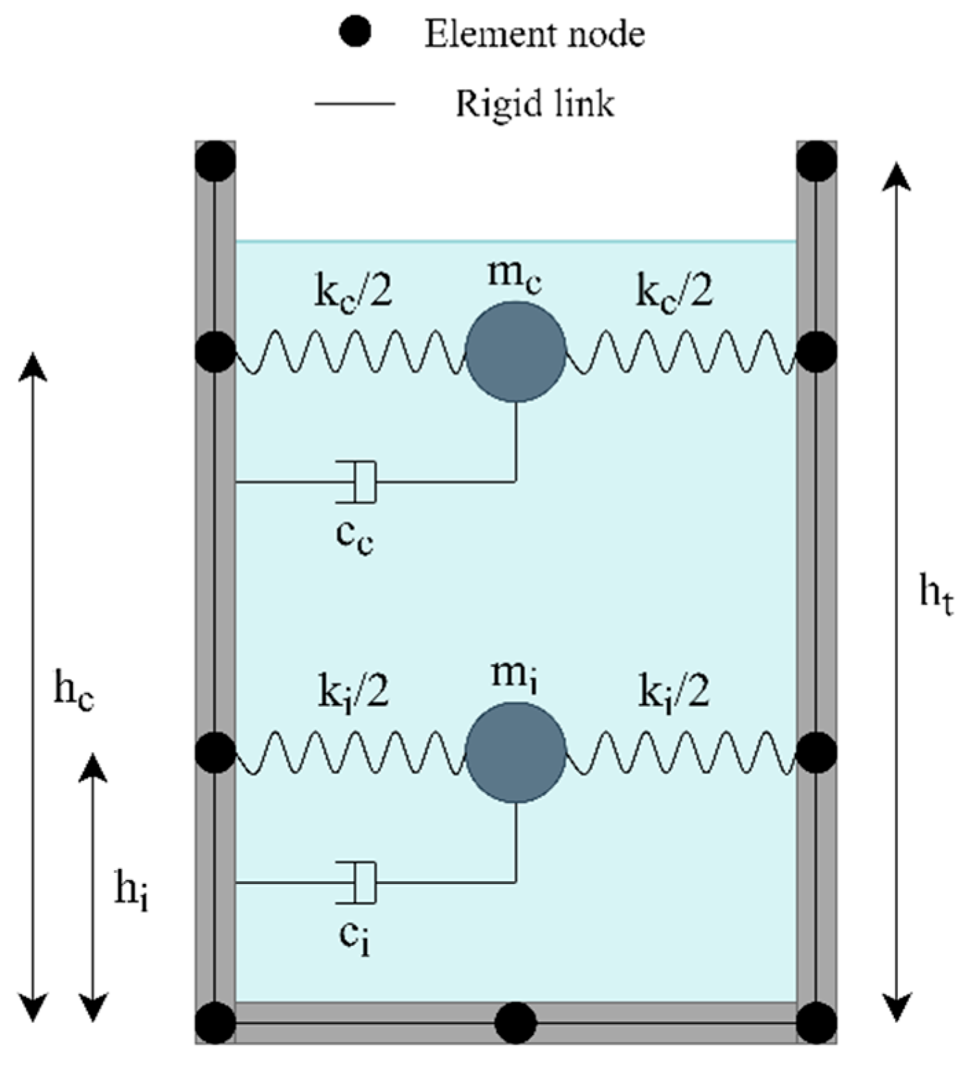
2. Tank Numerical Models

2.1. Anchored Steel Storage Tanks

For this study, a set of 60 anchored cylindrical steel storage tanks was selected for each seismic zone. These tanks have a diameter-to-height (D/H) ratio ranging from 0.8 to 3.5 and feature varying wall thicknesses along their height. The tanks were designed in accordance with EC8 Part 4 [18] and EC3-1-6 [19]. The complete list of the designed tanks adopted in this study is presented in Appendix A. The tank models were developed based on Malhotra’s [8,9] simplified model for cylindrical tanks, with numerical simulations conducted in OpenSeesPy [20] to perform dynamic time-history analyses. Notably, Malhotra’s model is also incorporated into European seismic design standards, specifically EC8 Part 4—Annex A [18].
Malhotra’s [8,9] system employs a small number of uncoupled degrees of freedom, each representing a different vibration mode of the fluid-structure system (Figure 2). These modes are analyzed independently, and their responses are then combined using a selected modal combination rule in case of response spectrum analysis or summed up if time-history analyses are performed. The single-degree-of-freedom (SDoF) model accounts for the impulsive mass (representing the impulsive mode), convective masses (sufficient to capture at least 98% of the participating mass of liquid inside the tank), and the mass of the steel tank structure. Each of these masses is assigned a specific height, as defined by the simplified model, and is connected to the tank walls via springs and dashpots. These equivalent heights are necessary to consider the overturning effects. Meanwhile, the tank walls and base plate are modeled using rigid links. The periods of the impulsive and first convective component are defined as follows:
T i m p = C i ρ H t w / R E
T c o n , 1 = C c R
where R is the radius of the tank, H represents the design height of the liquid, ρ is the mass density of the stored liquid, tw denotes the uniform equivalent thickness of the tank wall, and E is the elastic modulus of the tank material. The coefficients Ci and Cc can be derived from [9] or [18].
A key distinction between Malhotra’s original model [8,9] and the one adopted in this study is that the latter includes three convective modes, enhancing its accuracy.
Hence, the total base shear F is defined as
F = ( m i + m w + m r ) a i m p + m c , i a c o n , i
where mi represents the mass of the impulsive component of the fluid, mc,i is the i-th convective component mass of the fluid, mw is the tank wall mass, mr is the mass of the tank roof, aimp is the impulsive acceleration, and acon,i is the acceleration associated with the i-th convective mode of vibration.
In addition, the overturning moments above and below the base plate can be computed by means of Equations (4) and (5), respectively:
M = ( m i h i + m w h w + m r h r ) a i m p + m c , i h c , i a c o n , i
M = ( m i h i + m w h w + m r h r ) a i m p + m c h c , i a c o n , i
In which hi and hc,i are the height of the centroid of the impulsive and i-th convective hydrodynamic wall pressures above the base plate; h’i and h’c,i are the height of the centroid of the impulsive and i-th convective hydrodynamic wall pressures below the base plate; hw and hr are the height of the centre of gravity of tank wall and roof, respectively. Both hi and hc, as well as h’i and h’c,i can be obtained from either [9] or [18].
Then, the wave height of the liquid surface due to sloshing is obtained by [18]:
d = 0.84 R a c o n , 1 / g
where g is the gravitational acceleration. It should be noted that the coefficient 0.84 is adopted for considering the first convective mode. If, instead of 0.84, a value of 1.0 is adopted, then the computed vertical displacement (wave height) will take into account the whole sloshing liquid moves in the first convective mode [21].
It should be noted that Equation (6) is based on a simplified representation of the first convective mode and does not account for the possible amplification effects due to higher-mode excitations. As highlighted in [22], such effects can significantly increase the vertical displacement of the liquid surface.
All tanks in the study set are made of S235 steel, and water is the stored liquid with a density (ρ) of 1.0 t/m3. Since the tanks are considered anchored to the ground, the base nodes are fully fixed to prevent uplift.

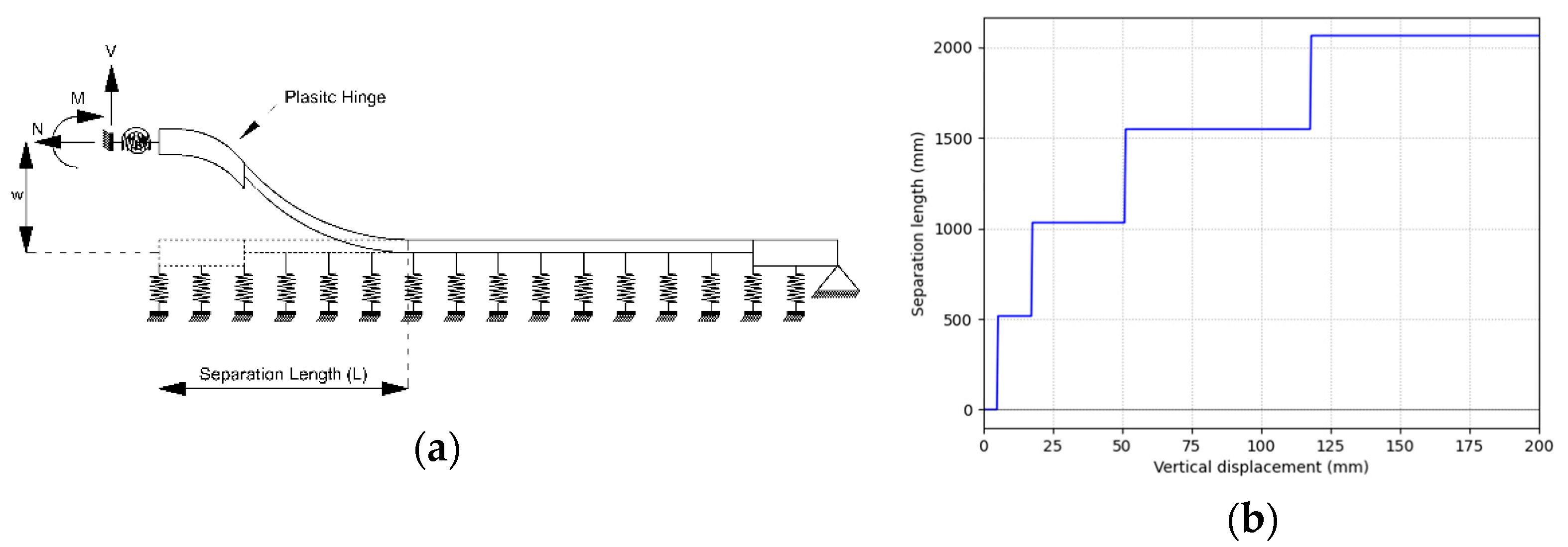
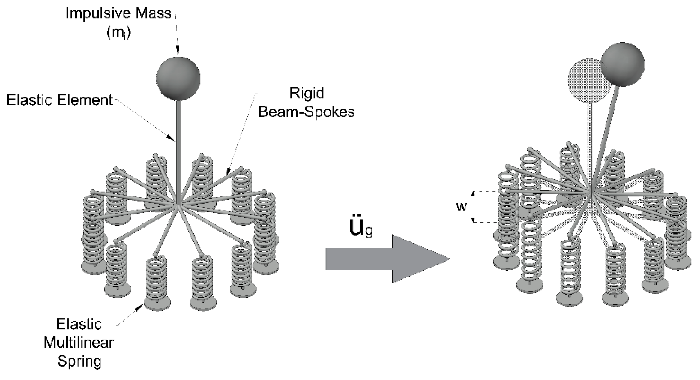
2.2. Unanchored Steel Storage Tanks

The second ground-structure connection configuration is modeled following the approach described by Bakalis et al. [23,24]. In this case, a set of 60 tanks, for each seismic zone, was analyzed without specific consideration of the D/H ratio, as unanchored configurations generally require squat tanks due to their inherent overturning stability. As well as for the anchored tanks, these sets of unanchored tanks were designed in accordance with EC8 Part 4 [18] and EC3-1-6 [19]. The complete list of the designed tanks adopted in this study is presented in Appendix A.
This model incorporates a multilinear relationship for the spring elements at the tank base to capture the uplift behavior of the base plate. To calibrate these multilinear springs, a detailed nonlinear analysis was performed for each tank’s base plate. The process begins with a static pushover analysis, in which a strip of the base plate is modelled using fiber elements (Figure 3a) to characterize its uplift response (Figure 3b). To simulate the interaction between the tank wall and the base plate, axial and rotational springs are introduced at one the strip’s end. The other end is instead hinged, since it represents the centroid of the tank’s base plate; taking advantage of the system symmetry, only half part of the base plate can be modeled.
The connection to the ground is represented by vertical springs that exhibit tensionless soil/foundation behavior. The pushover analysis results—specifically, the force-displacement and uplift-separation length curves (Figure 3b)—were used to calibrate the springs in the “Joystick” 3D tank model (Figure 4). In this model, the impulsive and convective masses are represented in the same manner as in the anchored tank configuration. Proper discretization of the base plate strip in the joystick model enhances the understanding of ground-tank interaction, particularly in three-dimensional simulations where seismic excitation occurs simultaneously in both horizontal directions.
It is important to note that, while the described model is suitable for capturing the nonlinearities associated with the uplift of the tank, it does not allow for accurate simulation of the dynamic impact effect occurring when the base plate lifts off and subsequently strikes the foundation.

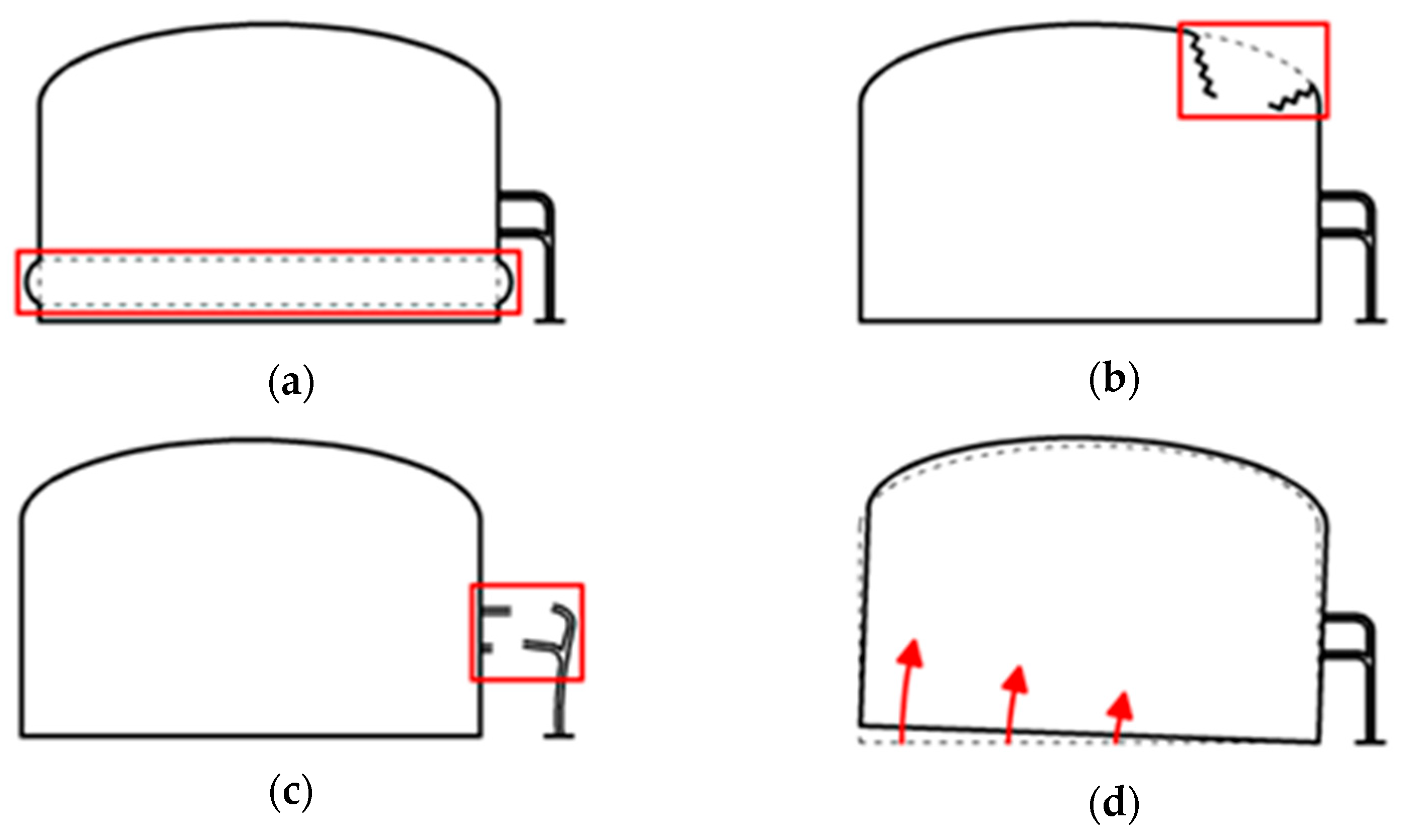
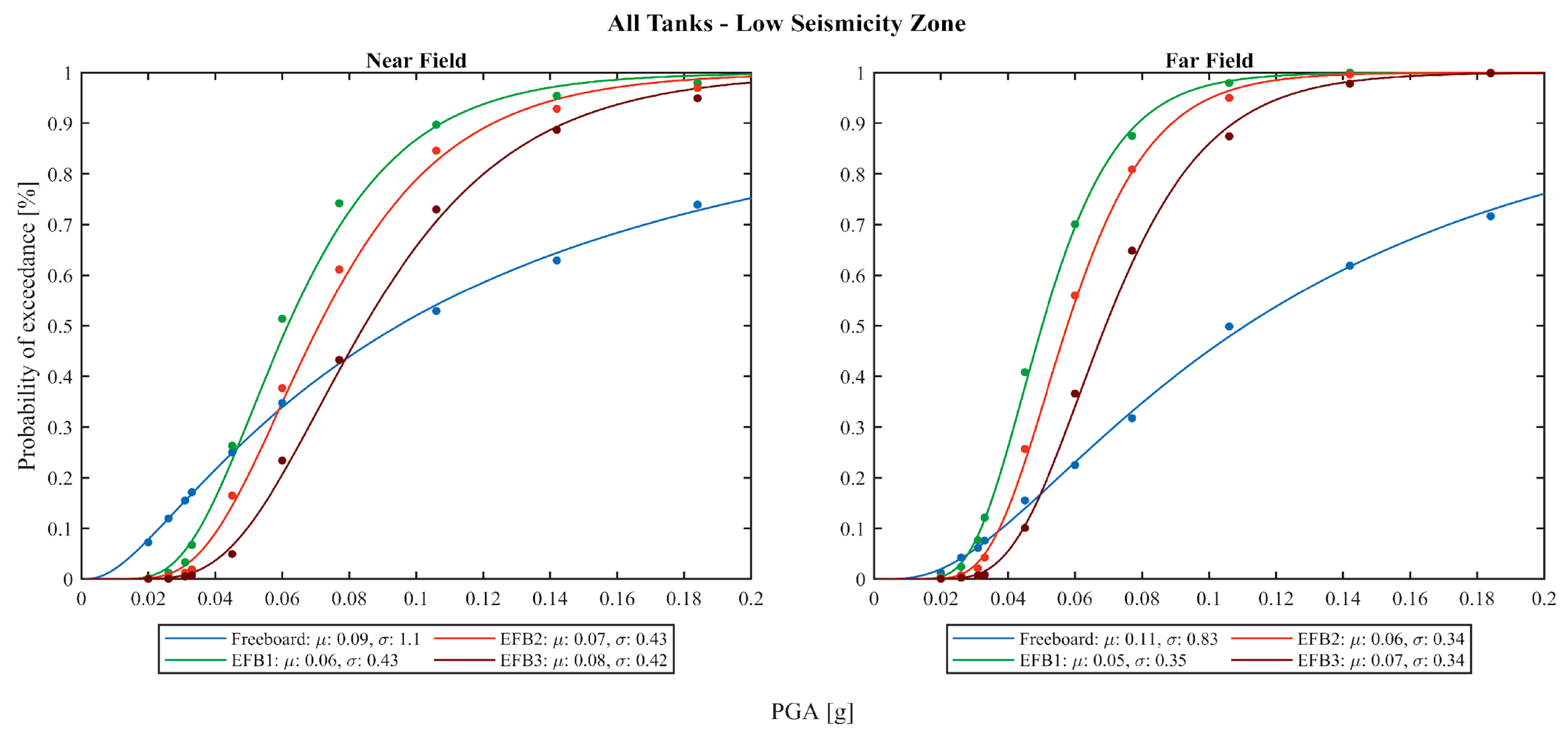
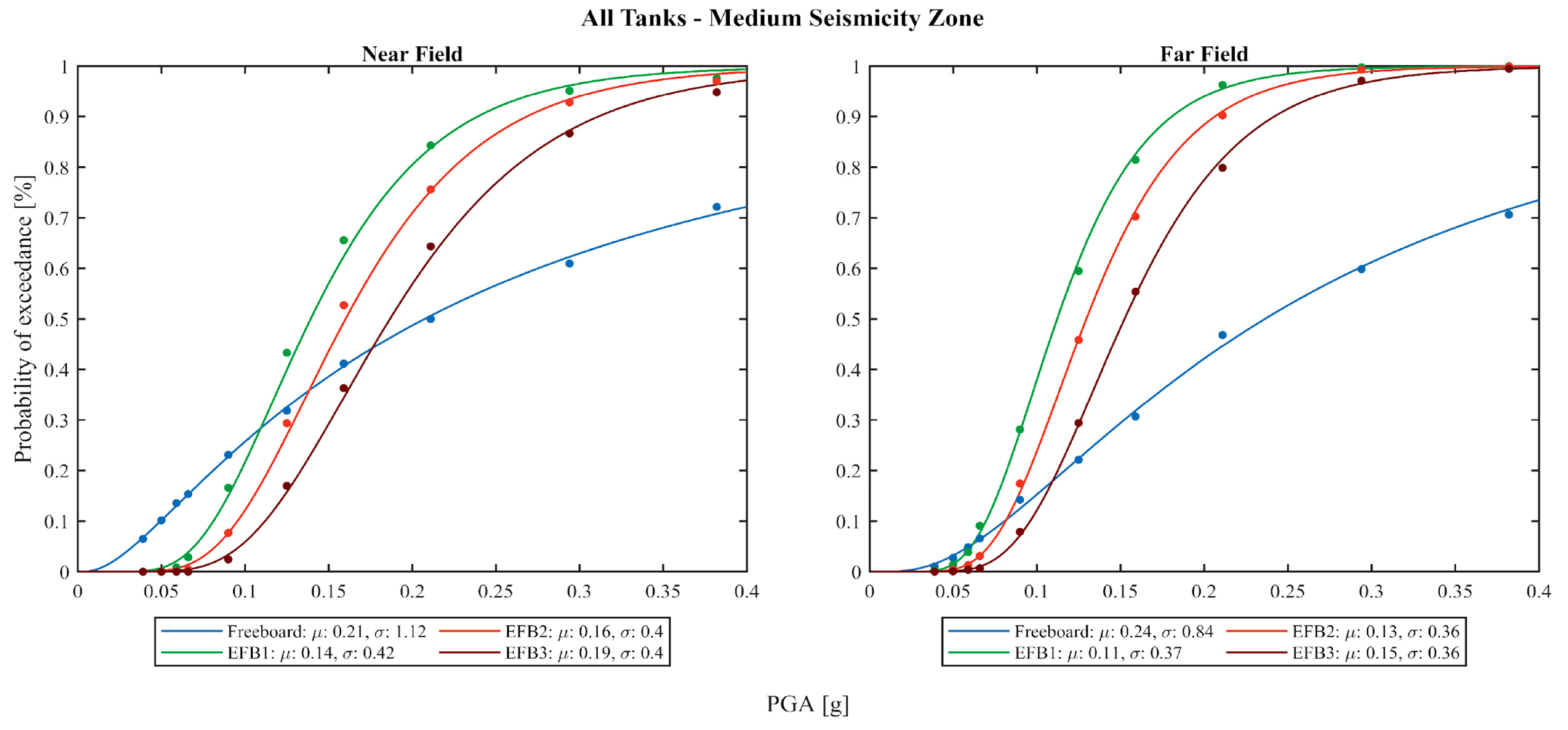
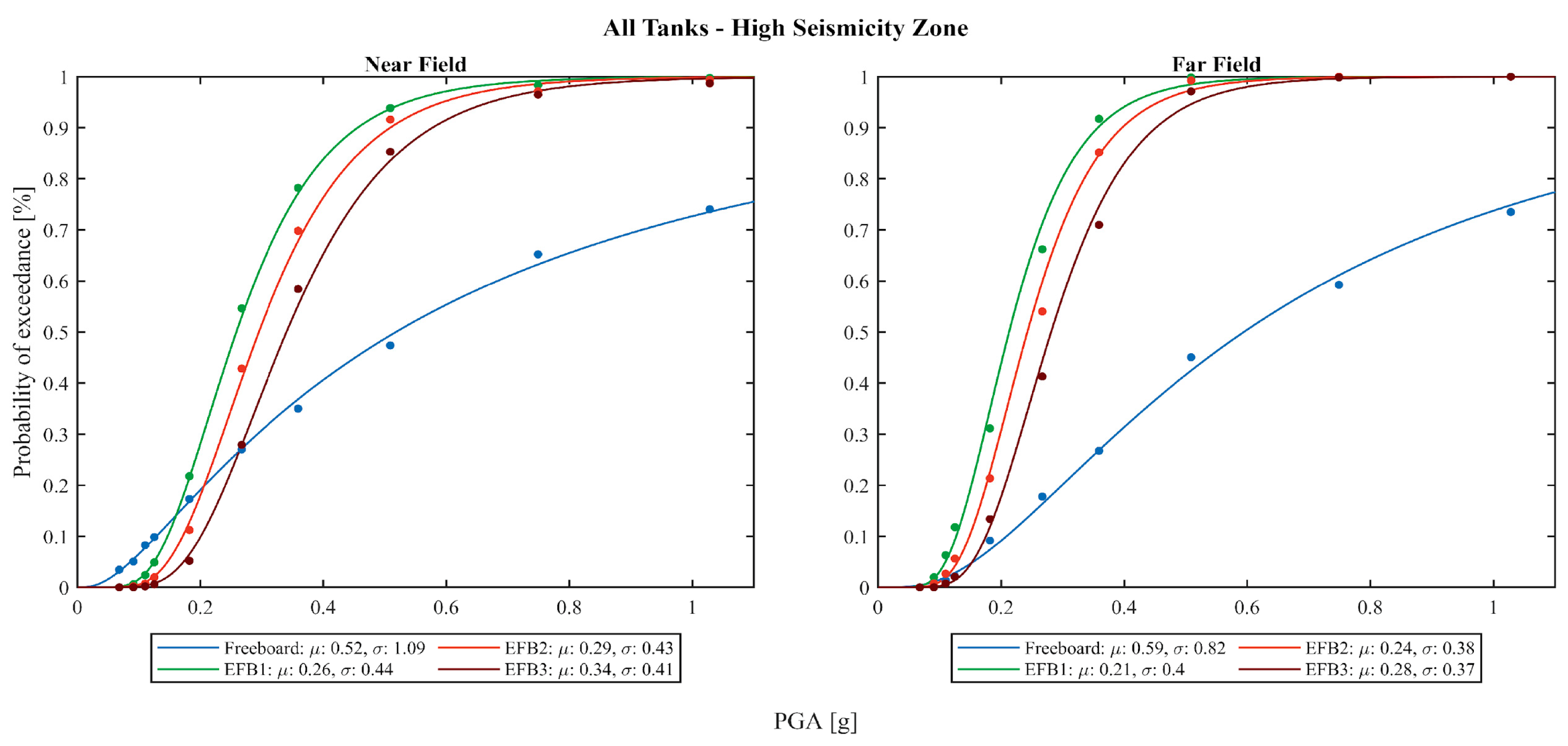
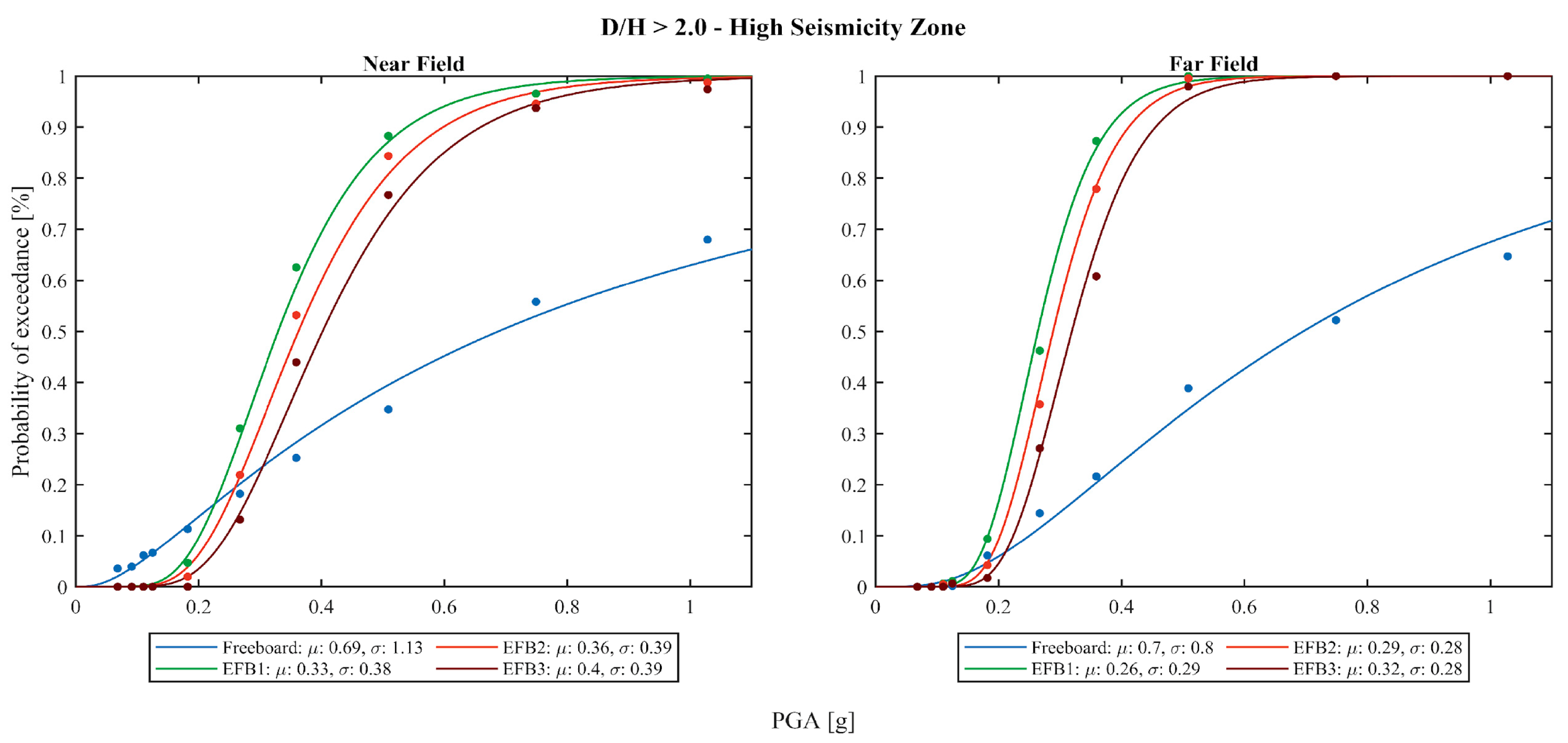
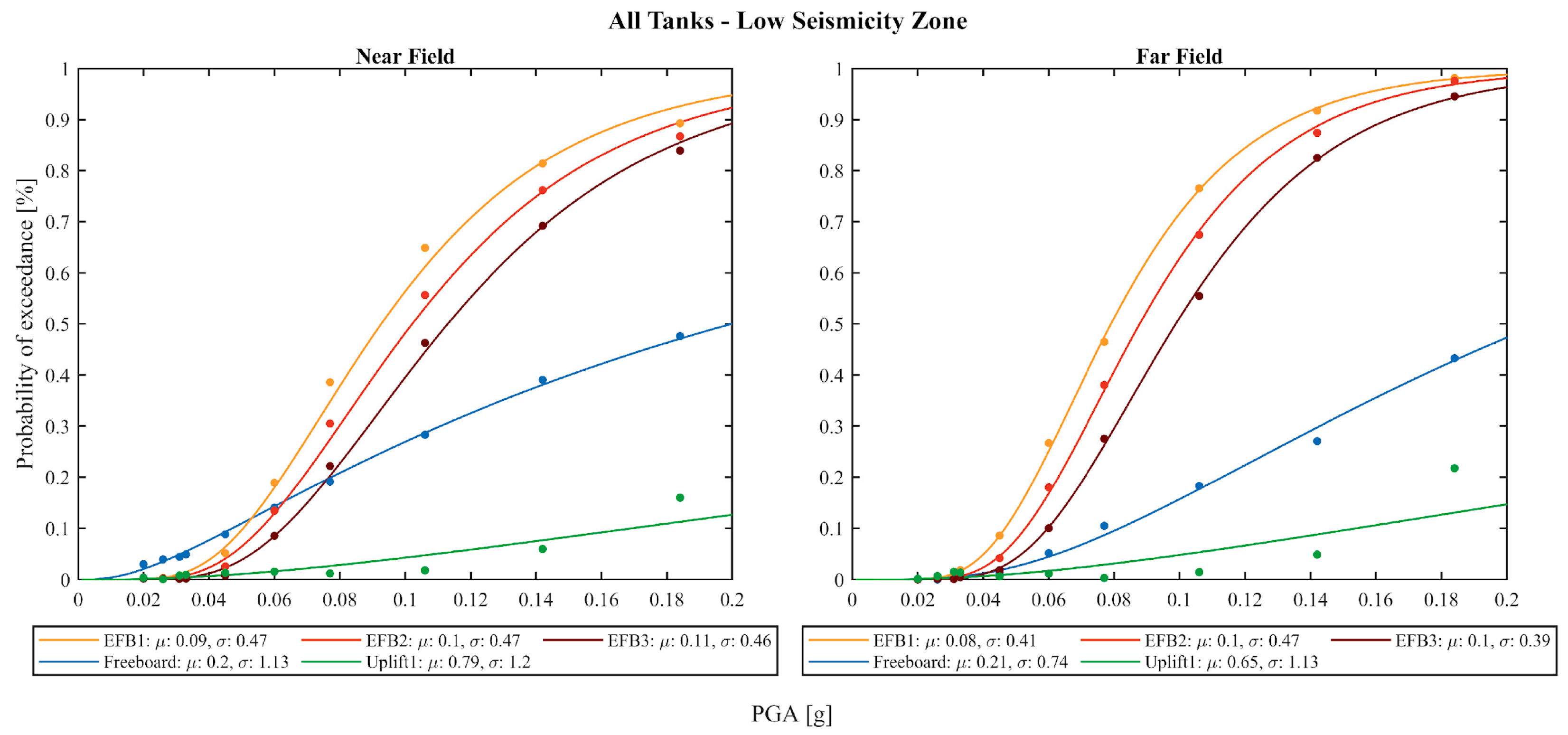
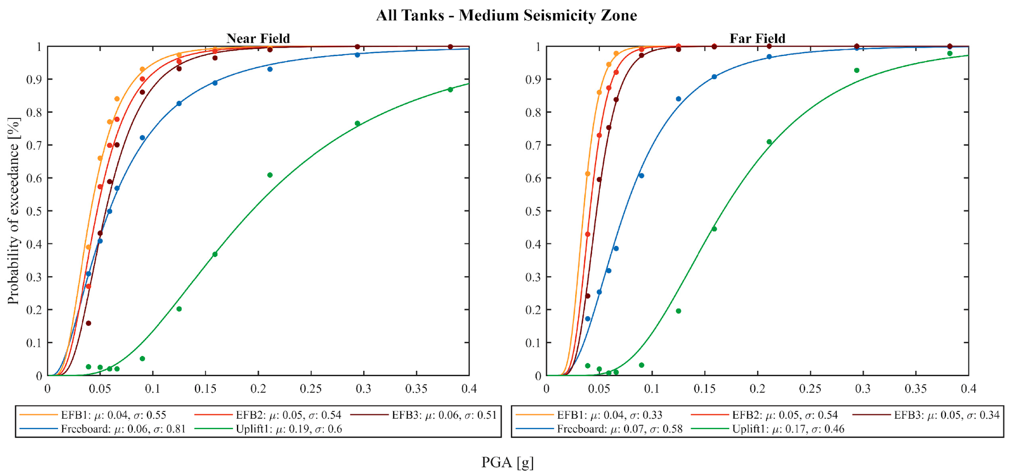
2.3. Damage States Definition

Numerous past studies have extensively investigated and identified the typical structural damages that commonly affect tank systems during seismic events [2,3,4,5,6]. These studies, based on both experimental and numerical analyses, as well as post-earthquake field observations, provide a comprehensive understanding of the vulnerabilities associated with such structures. Specifically, research conducted by Brunesi et al. [25] and Merino Vela et al. [26] highlighted that storage tanks are particularly susceptible to damage due to several key failure mechanisms. These include the formation of convective waves in the stored liquid (sloshing), yielding or complete failure of the anchorage system, and the development of localized wall instabilities, such as the well-documented elephant’s foot buckling (EFB).
In addition to damage characterization, further studies have also focused on defining appropriate criteria for the establishment of ad hoc limit states, which are essential for assessing seismic vulnerability [23,26,27,28,29,30]. For example, Bakalis et al. [23] and Merino Vela et al. [26] proposed specific limit state thresholds that account for different dominant failure mechanisms, including buckling-induced instabilities, damage resulting from excessive sloshing, and failures related to the anchorage system.
Building upon this existing body of knowledge, the present study adopts six distinct limit states (LSs) for the seismic vulnerability assessment of storage tanks:
  • Convective wave exceeding the freeboard;
  • Exceeding 80% of the Elephant Foot Buckling threshold (EFB1);
  • Exceeding 100% of the Elephant Foot Buckling threshold (EFB2);
  • Exceeding 140% of the Elephant Foot Buckling threshold (EFB3);
  • Tank uplift (for the unanchored configuration);
  • Tank overturning (for the unanchored configuration).
It is important to note that the last damage state—tank overturning—has not been observed within the considered PGA range. These limit states were carefully selected to comprehensively capture the critical failure modes that influence the structural integrity of tanks subjected to seismic loads.
Notably, sloshing waves are associated with the excitation of convective modes, whereas impulsive and convective modes influence wall stresses. However, elephant foot buckling has been found to correlate strongly with impulsive mode excitation [28].
The first LS pertains to the scenario in which the sloshing wave height reaches or surpasses the freeboard height. When this occurs, it can result in structural damage to the upper sections of the tank due to the impact of fluid against the tank’s shell or roof. Additionally, in the case of open-top tanks, this phenomenon can lead to fluid spillover, posing further risks. Previous studies, such as the investigation by Merino Vela et al. [31], identified this mechanism as a key driver of fragility in the analyzed special concentrically braced frame-tank system. Notably, this study evaluated the tanks as non-structural elements, where seismic demand is significantly influenced by the response of the primary building [6,26,31,32].
According to this framework, the sloshing wave height can be determined using Equation (6). Meanwhile, the freeboard height—considered the “capacity” parameter for evaluating the attainment of this limit state—is assumed to be the difference between the height of the tank (ht) and liquid height (H). Based on this formulation, the freeboard height (f) is determined for each tank, as expressed in Equation (7).
d = 0.84 R a c o n , 1 g < f
Concerning the Elephant Foot Buckling LSs, it should be noted that this is verified by changing the recorded seismic forces into stresses for comparison with the critical buckling stress limit. The development of the elephant’s foot buckling (EFB) mechanism, typically occurring near the base of the tank’s wall, can lead to severe consequences, including irreversible deformation of the tank walls and potential leakage of hazardous substances or stored fluids. This failure mode, which exhibits elastic–plastic behavior, has been widely observed during seismic events [2,3,4,5,6,25] and is primarily attributed to the combined effects of axial compression and internal pressure. These interacting forces generate circumferential tension perpendicular to the axial compression, a condition that is further exacerbated by earthquake-induced inertial forces acting on the structure.
Design provisions aimed at mitigating EFB failure are well-established and have been incorporated into various international standards governing the design of tanks and silos [18,19]). These standards commonly rely on analytical formulations originally developed by Rotter [33] to assess and predict the onset of this failure mechanism. In addition to design considerations, several strengthening techniques have been proposed to enhance the structural resilience of tanks against EFB [7,34], with these methodologies being grounded in detailed analytical evaluations. Specifically, the EFB verification can be determined using the following equations, as prescribed in EN-1993-1-6 [19].
σ i d , E d = σ x , E d σ x , R d k x k i σ x , E d σ x , R d σ θ , E d σ θ , R d + σ θ , E d σ θ , R d k θ + τ x θ , E d τ x θ , R d k τ 1
where k x , k θ , and k τ are interaction buckling factors, σ θ , E d , σ x , E d , and τ x θ , E d represent the design maximum values of the membrane stresses in compression and shear, determined using a linear elastic analysis of the tank and, under axisymmetric conditions, also the membrane theory. The design buckling resistances for the meridional stress σ x , R d , the circumferential stress σ θ , R d , and the shear stress τ x θ , R d are respectively
σ x , R d = σ x , R k γ M
σ θ , R d = σ θ , R k γ M
τ x θ , R d = τ x θ , R k γ M
where γ M ≥ 1.1 is the partial resistance factor, and σ x , R k is the characteristic buckling stress for the meridional stress, σ θ , R k for the circumferential stress, and τ x θ , R k for the shear stress. More information on this approach can be found in EC3-1-6 [19]. To account for varying degrees of structural damage, three threshold levels were defined for the EFB failure mode, corresponding to 80%, 100%, and 140% of the critical buckling stress. This approach allows for a more detailed assessment of seismic vulnerability, as it captures both initial yielding and severe buckling conditions. Similar multi-level definitions, although for different LSs, have been adopted in previous fragility-based studies [25,26,31] to better represent the progressive nature of damage.
Finally, the limit states related to uplift and overall instability of the tanks due to structural overturning have been defined by calculating the anchorage ratio J -factor, following the API Standard 650 [35]. It is important to note that, despite its simplified nature, this approach is the only one that allows for considering and simulating the uplift and overall instability of the tank when adopting the Malhotra model. The anchorage ratio J is determined using Equation E.6.2.1.1.1-1 from API Standard 650 [35], which is also presented in Equation (12).
J = M b D 2 w t 1 0.4 A v + w a F p w i n t
where M b denotes the bending moment acting beneath the tank’s base (as given in Equation (5)), D refers to the diameter of the tank, and A v represents the vertical earthquake acceleration parameter, which is assumed to be 90% of the impulsive acceleration in this study [36]. The term w a is the force resisting uplift in the annular region, while F p indicates the ratio of nominal operating pressure to design pressure, with a minimum value of 0.4. Additionally, w i n t refers to the calculated design uplift load per unit circumferential length due to design pressure, which is zero for tanks that are unpressurized. The total weight per unit length along the circumference w t is calculated using Equation (13).
w t = W s π D + w r s
where W s is the total weight of the tank walls, and w r s is the roof load acting on the walls. The calculation of the anchorage ratio J (Equation (12)) helps determine the occurrence of uplift or global instability based on specific thresholds outlined in Table E.6 of API Standard 650 [35], which are also presented in Table 1.

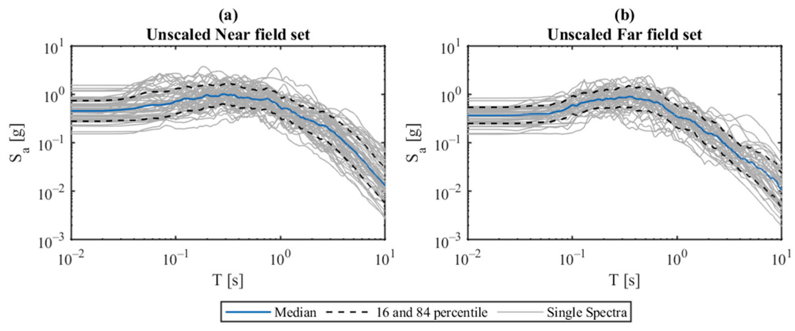
3. Seismic Hazard and Record Selection

As previously mentioned, the two sets of tanks (anchored and unanchored) were analyzed for three Italian seismic zones, representing low, medium, and high seismicity. These zones correspond to peak ground acceleration (PGA) values of 0.06 g, 0.125 g, and 0.267 g, respectively, for a return period of 475 years, as specified by the Italian National Standard [37].
To maximize the excitation of different periods as the impulsive and convective ones, and consequently, their associated damage states, the Far-field and Near-field ground motion sets from FEMA P695 [38] were used (Figure 5). These sets consist of 22 and 28 records, respectively. Each accelerogram was scaled to match the PGA values defined by the NTC18 [37]. In this study, PGA was chosen as the intensity measure (IM). It should be mentioned that not all the selected ground motions, after PGA scaling, fully conform to the expected spectral shapes of Near-field and Far-field events, which may influence the results. In addition to the adoption of different IMs, future studies will also consider the aforementioned aspect to enhance consistency. However, it is well known that selecting a different IM could yield varying results. For instance, adopting PGA or spectral acceleration at the impulsive period, Sa(Timp), effectively excites the impulsive component, leading to a suitable evaluation of the EFB. Conversely, sloshing is associated with the convective component, making the use of spectral acceleration at convective period, Sa(Tconv), more appropriate. Regarding the latter IM, it should be noted that Tconv varies significantly across different tanks, making a seismic assessment based on a taxonomy of tanks challenging. In contrast, Timp typically falls within a narrower range, allowing it to be more readily used as an IM. With this in mind, future research will explore alternative IMs, such as the Average Spectral Acceleration (AvgSA) or Peak Ground Velocity (PGV).
For the vulnerability analysis, 10 return periods were considered: 30, 50, 72, 98, 224, 475, 975, 2475, 4975, and 9975 years. Nonlinear time-history analyses were then performed using 50 pairs of records (22 for the Far-field and 28 for the Near-field sets) across the 10 return periods for the three seismic zones, resulting in a total of 90,000 simulations. The analyses were carried out in OpenSeesPy [20], using the implicit Hilber–Hughes–Taylor (HHT) time integration method with an alpha coefficient of 0.9. Convergence at each iteration was verified through the energy-based convergence criterion available in OpenSeesPy [20]. During each analysis step, the accelerations at the defined masses were recorded. These were used to compute the seismic forces and overturning moments, from which the pressure distribution along the height of the tank’s walls was derived. With the seismic demand fully characterized, the exceedance of each defined LS was assessed. Each simulation provided information on the number and type of LS exceeded, enabling the construction of fragility functions. These functions were fitted using a maximum likelihood method, assuming a lognormal distribution defined by median (μ) and standard deviation (σ). In addition, it should be noted that the analyses were performed under the conditions of small deformations.

4. Results of the Dynamic Analyses

Based on the results of the time-history analyses, fragility curves were developed for both tank configurations. The intensity measure (IM) used was PGA (in g), and the previously defined damage states (Section 2.3) were adopted as limit states (LSs). The resulting fragility curves follow a lognormal distribution, which describes the probability of exceeding a given LS. Two key parameters are provided: the median (μ), representing the IM value at which there is a 50% probability of exceeding the LS; and the dispersion (σ), indicating the variability of the curve.
The results are first disaggregated by diameter-to-height (D/H) ratio and then presented as an overall dataset incorporating all tanks. Results for all seismic zones are shown by aggregating the different D/H configurations. However, for the high-seismicity zone, additional results are provided specifically for tanks with D/H ratios greater than 2.
It is important to note that, for both tank types, the Freeboard LS represents a minor damage level, as it corresponds to the liquid impacting the tank’s roof. While this impact may cause damage to the roof structure, it does not indicate a complete tank failure. Therefore, the following discussion primarily focuses on the elephant foot buckling limit states.

4.1. Anchored Tanks Results

Across all analyses conducted, the fragility curves for the different levels of elephant foot buckling (EFB1, EFB2, and EFB3) exhibit an expected trend: the intensity measure (IM) required to reach each limit state (LS) increases as the severity of the LS increases.
For the low-seismicity zone (Figure 6), the Freeboard LS is characterized by median (μ) values of 0.09 g and 0.11 g, with dispersions (σ) of 1.1 and 0.83 for the Near-field and Far-field sets, respectively. The EFB1 LS is reached at μ values of 0.06 g and 0.05 g, with σ values of 0.43 and 0.35 for Near-field and Far-field, respectively. Similar but slightly higher values are observed for EFB2 and EFB3. In both sets of records, EFB represents the most vulnerable LS, consistent with findings from similar studies [23].
For the medium-seismicity zone (Figure 7), a comparable pattern is observed. EFB1 occurs at μ = 0.14 g and 0.11 g, with σ = 0.42 and 0.37 for Near-field and Far-field, respectively. The EFB2 and EFB3 LSs have μ values of 0.16 g and 0.19 g with σ = 0.4 for the Near-field set, while the Far-field set yields μ = 0.13 g and 0.15 g, with σ = 0.36. The Freeboard LS is reached at μ = 0.21 g and 0.24 g, with σ = 1.12 and 0.84 for Near-field and Far-field, respectively. Notably, the dispersion of results is lower for the Far-field set, indicating that it more consistently excites the different damage states of the tanks.
In the high-seismicity zones (Figure 8 and Figure 9), the trend of LS exceedance remains consistent. The most vulnerable LS—80% of elephant foot buckling (EFB1)—has a 50% probability of being reached at a PGA of 0.21 g for the Far-field set and 0.26 g for the Near-field set (Figure 8). While the PGA difference between the two sets is not significant, the Far-field set exhibits lower dispersion, particularly for tanks with a D/H ratio greater than 2 (Figure 9). For these tanks, the Freeboard LS occurs at similar μ values (0.69 g and 0.7 g), but the dispersion (σ) decreases from 1.13 for the Near-field set to 0.8 for the Far-field set.
Overall, these results highlight the impact of accelerogram selection. This underscores that seismic demand is not solely dependent on the PGA value but is strongly influenced by the spectral characteristics of each accelerogram. Therefore, selecting records that are representative of the seismic scenario is essential for robust fragility assessment. The FEMA Far-field set, characterized by a higher frequency content, primarily excites the impulsive mass of the liquid, leading to lower μ values for a given PGA. Conversely, the Near-field set induces slightly greater excitation of the convective masses, albeit with higher dispersion in the results.

4.2. Unanchored Tanks Results

For the low-seismicity zone (Figure 10), the combination of conservative design and low seismic demand resulted in very few exceedances of the Uplift and Freeboard limit states (LSs). Given that the maximum PGA for this site is below 0.19 g and the median (μ) values for these LSs exceed 0.2 g (e.g., 0.79 g for Uplift in the Near-field case), the probability of reaching these LSs is minimal. However, the median values for the Elephant Foot Buckling (EFB) LSs are around 1 g, indicating that unanchored tanks are significantly prone to this failure mode.
For tanks in the medium-seismicity zone, the fragility curves exhibit a steep trend for all LSs except for Uplift. As shown in Figure 11, Uplift occurs at μ values of 0.17 g and 0.19 g, whereas other LSs fall within the range of 0.04 g to 0.07 g. This suggests that, in terms of probability, Uplift remains significantly lower compared to other LSs.
For tanks in the high-seismicity zone (Figure 12), the Freeboard LS has a 50% probability of exceedance at μ values of 0.49 g and 0.56 g, which is notably higher than the Uplift LS, occurring at μ = 0.35 g and 0.32 g for the Near-field and Far-field sets, respectively. This shift in the sequence of LS exceedance—where Uplift becomes more vulnerable than Freeboard compared to the medium-seismicity zone—can be attributed to the conservative design approach for Freeboard height under high seismic demands. In fact, Freeboard height directly influences the Freeboard LS, and the standard methods used for defining this height tend to be oversimplified. Time-history analyses, however, provide a more accurate representation of the seismic response.
In general, unanchored tanks exhibit trends similar to anchored tanks, with greater susceptibility to Elephant Foot Buckling than to Freeboard or Uplift LSs. Additionally, higher dispersion (σ) is observed for the Near-field set, along with minor variations in median (μ) values.

5. Conclusions

This study aimed to evaluate the impact of different ground motion record sets—Far-field and Near-field, as defined in FEMA P695 [38]—on seismic vulnerability assessment of steel storage tanks. The identified damage states are closely linked to the tank’s vibration modes, namely the impulsive mode (associated with short periods) and the convective mode (associated with longer periods). The impulsive mode is typically excited by ground motions with higher frequency content (as in Far-field records), whereas convective modes are more affected by low-frequency components or long-duration pulses (often found in Near-field records).
Two tank configurations were considered: anchored and unanchored. In the latter case, overturning stability is ensured by the tank’s self-weight.
Preliminary results indicate that seismic vulnerability, in terms of the median values of fragility curves, does not exhibit significant variations between the two record sets. However, the dispersion of results is notably lower when using Far-field records. The greater dispersion observed for Near-field records is attributed to their irregular spectral content and the presence of velocity pulses, which can lead to highly variable structural responses in liquid-storage tanks. This behavior particularly affects the convective and impulsive modes, resulting in increased variability in the seismic demand across the record set.
Further analyses are needed to validate these findings, including the incorporation of alternative intensity measures such as the Average Spectral Acceleration (AvgSA) or Peak Ground Velocity (PGV) in combination with both Near- and Far-field records.

Author Contributions

Conceptualization, G.G. and R.R.M.; methodology, G.G. and R.N.; software, G.G. and A.R.; validation, G.G. and R.R.M.; formal analysis, A.R.; investigation, G.G. and A.R.; resources, R.N.; data curation, R.R.M.; writing—original draft preparation, G.G. and A.R.; writing—review and editing, G.G., A.R., R.R.M. and R.N.; visualization, A.R.; supervision, G.G.; project administration, R.N.; funding acquisition, R.N. All authors have read and agreed to the published version of the manuscript.

Funding

The authors gratefully acknowledge the Italian Department of Civil Protection (DPC) for their financial contributions to this study through the 2023−2024 Project (Work Package 15).

Institutional Review Board Statement

Not applicable.

Informed Consent Statement

Not applicable.

Data Availability Statement

The original contributions presented in this study are included in the article. Further inquiries can be directed to the corresponding author.

Conflicts of Interest

The authors declare no conflicts of interest.

Appendix A

This section presents the complete list of tanks designed and adopted for the analyses performed. In the following tables (Table A1 and Table A2), D is the diameter, H is the liquid height, t is the equivalent thickness of the tank’s walls, and fy is the yielding strength of the steel adopted for the tank.
Table A1. Designed anchored tanks.
Anchored TankLow Seismic ZoneMedium Seismic ZoneHigh Seismic Zone
D [m]H [m]t [mm]fy [N/mm2]D [m]H [m]t [mm]fy [N/mm2]D [m]H [m]t [mm]fy [N/mm2]
15.05.02.02355.04.83.02355.04.43.0235
26.06.03.02356.05.83.02356.05.34.0235
37.07.03.02357.06.84.02357.06.35.0235
48.08.04.02358.07.85.02358.07.26.0235
59.09.05.02359.08.86.02359.08.27.0235
610.010.05.023510.09.87.023510.09.28.0235
711.011.06.023511.010.88.023511.010.210.0235
812.012.07.023512.011.89.023512.010.710.0235
913.013.08.023513.012.810.023513.011.210.8235
1014.014.09.023514.013.812.023514.012.112.0235
1115.015.010.023515.014.813.023515.012.412.7235
1216.016.011.023516.015.814.023516.013.213.7235
1317.017.012.023517.016.815.023517.014.115.0235
1418.018.013.023518.016.215.023518.013.414.7235
1519.019.014.023519.017.116.023519.014.216.0235
1620.020.015.023520.017.116.723520.014.016.3235
1721.021.016.023521.018.018.023521.013.816.6235
1822.022.017.023522.018.819.023522.014.518.6235
1923.023.018.023523.018.619.623523.015.120.0235
2024.024.019.023524.018.319.623524.014.719.6235
2125.024.921.023525.019.121.023525.015.321.0235
2226.025.922.023526.019.822.023526.014.820.7235
2327.025.722.123527.019.322.123527.015.321.6235
2428.026.623.523528.020.023.523528.015.923.0235
2529.027.625.023529.020.724.523529.016.424.0235
2630.027.125.023530.020.024.023530.015.623.5235
2731.026.625.523531.020.725.523531.016.124.4235
2832.027.426.523532.021.327.023532.016.625.9235
2933.028.328.023533.021.928.023533.017.126.9235
3034.027.527.823534.021.027.323534.017.528.4235
3135.028.329.423535.021.628.823535.018.029.4235
3236.027.428.823536.022.230.023536.016.928.2235
3337.028.230.423537.021.029.123537.017.329.1235
3438.028.932.023538.021.630.123538.017.730.7235
3539.027.831.723539.022.131.723539.018.233.0235
3640.028.532.623540.022.732.623540.016.830.6235
3741.029.234.323541.023.234.323541.017.232.2235
3842.027.933.323542.021.832.223542.017.533.6235
3943.028.534.623543.022.333.823543.017.934.6235
4044.029.236.323544.022.834.823544.018.336.3235
4145.029.838.023545.023.336.523545.018.738.0235
4246.030.539.023546.023.838.223546.019.139.0235
4347.028.937.623547.024.239.223547.017.336.0235
4448.029.539.223548.022.536.823548.017.636.8235
4549.030.141.023549.022.938.523549.018.038.5235
4650.028.339.523550.023.439.523550.018.339.5235
4751.028.840.423551.023.841.323551.018.741.3235
4852.029.442.223552.024.242.223552.019.043.1235
4953.029.944.123553.024.744.123553.019.344.1235
5054.030.545.023554.022.640.523554.017.239.6235
5155.028.443.223555.023.042.323555.017.440.5235
5256.028.944.223556.023.343.223556.017.742.3235
5357.029.446.123557.023.745.123557.018.043.2235
5458.029.947.023558.024.146.123558.018.345.1235
5559.030.449.023559.024.548.023559.018.647.0235
5660.030.950.023560.024.949.023560.018.948.0235
5761.028.446.923561.022.445.023561.019.250.0235
5862.028.948.923562.022.846.823562.019.551.0235
5963.029.349.823563.023.147.723563.019.853.0235
6064.029.851.823564.023.448.623564.020.154.0235
Table A2. Designed unanchored tanks.
Unanchored TankLow Seismic ZoneMedium Seismic ZoneHigh Seismic Zone
D [m]H [m]t [mm]fy [N/mm2]D [m]H [m]t [mm]fy [N/mm2]D [m]H [m]t [mm]fy [N/mm2]
15.04.83.02355.05.02.02355.04.43.0235
26.05.83.02356.06.03.02356.05.34.0235
37.06.84.02357.07.03.02357.06.35.0235
48.07.85.02358.08.04.02358.07.26.0235
59.08.86.02359.09.05.02359.08.27.0235
610.09.87.023510.010.05.023510.09.28.0235
711.010.88.023511.011.06.023511.010.210.0235
812.011.89.023512.012.07.023512.010.710.0235
913.012.810.023513.013.08.023513.011.210.8235
1014.013.812.023514.014.09.023514.012.112.0235
1115.014.813.023515.015.010.023515.012.412.7235
1216.015.814.023516.016.011.023516.013.213.7235
1317.016.815.023517.017.012.023517.014.115.0235
1418.016.215.023518.018.013.023518.013.414.7235
1519.017.116.023519.019.014.023519.014.216.0235
1620.017.116.723520.020.015.023520.014.016.3235
1721.018.018.023521.021.016.023521.013.816.6235
1822.018.819.023522.022.017.023522.014.518.6235
1923.018.619.623523.023.018.023523.015.120.0235
2024.018.319.623524.024.019.023524.014.719.6235
2125.019.121.023525.024.921.023525.015.321.0235
2226.019.822.023526.025.922.023526.014.820.7235
2327.019.322.123527.025.722.123527.015.321.6235
2428.020.023.523528.026.623.523528.015.923.0235
2529.020.724.523529.027.625.023529.016.424.0235
2630.020.024.023530.027.125.023530.015.623.5235
2731.020.725.523531.026.625.523531.016.124.4235
2832.021.327.023532.027.426.523532.016.625.9235
2933.021.928.023533.028.328.023533.017.126.9235
3034.021.027.323534.027.527.823534.017.528.4235
3135.021.628.823535.028.329.423535.018.029.4235
3236.022.230.023536.027.428.823536.016.928.2235
3337.021.029.123537.028.230.423537.017.329.1235
3438.021.630.123538.028.932.023538.017.730.7235
3539.022.131.723539.027.831.723539.018.233.0235
3640.022.732.623540.028.532.623540.016.830.6235
3741.023.234.323541.029.234.323541.017.232.2235
3842.021.832.223542.027.933.323542.017.533.6235
3943.022.333.823543.028.534.623543.017.934.6235
4044.022.834.823544.029.236.323544.018.336.3235
4145.023.336.523545.029.838.023545.018.738.0235
4246.023.838.223546.030.539.023546.019.139.0235
4347.024.239.223547.028.937.623547.017.336.0235
4448.022.536.823548.029.539.223548.017.636.8235
4549.022.938.523549.030.141.023549.018.038.5235
4650.023.439.523550.028.339.523550.018.339.5235
4751.023.841.323551.028.840.423551.018.741.3235
4852.024.242.223552.029.442.223552.019.043.1235
4953.024.744.123553.029.944.123553.019.344.1235
5054.022.640.523554.030.545.023554.017.239.6235
5155.023.042.323555.028.443.223555.017.440.5235
5256.023.343.223556.028.944.223556.017.742.3235
5357.023.745.123557.029.446.123557.018.043.2235
5458.024.146.123558.029.947.023558.018.345.1235
5559.024.548.023559.030.449.023559.018.647.0235
5660.024.949.023560.030.950.023560.018.948.0235
5761.022.445.023561.028.446.923561.019.250.0235
5862.022.846.823562.028.948.923562.019.551.0235
5963.023.147.723563.029.349.823563.019.853.0235
6064.023.448.623564.029.851.823564.020.154.0235

References

  1. Van Loenhout, J.; Below, R. Human Cost of Disasters: An Overview of the Last 20 Years 2000–2019; Centre of Research on the Epidemiology of Disasters—United Nations Office for Disaster Risk Reduction: Brussels, Belgium, 2021. [Google Scholar]
  2. Yazdanian, M.; Ingham, J.M.; Lomax, W.; Wood, R.; Dizhur, D. Damage observations and remedial options for approximately 1500 legged and flat-based liquid storage tanks following the 2016 Kaikōura earthquake. Structures 2020, 24, 357–376. [Google Scholar] [CrossRef]
  3. Grajales-Ortiz, C.; Melissianos, V.E.; Bakalis, K.; Kohrangi, M.; Vamvatsikos, D.; Bazzurro, P. Relationships between earthquake-induced damage and material release for liquid storage tanks. In Proceedings of the 18th World Conference on Earthquake Engineering, Milan, Italy, 30 June–5 July 2024. [Google Scholar]
  4. Bevere, L.; Ewald, M.; Wunderlich, S. A Decade of Major Earthquakes: Lessons for Business; Swiss Re Institute: Zurich, Switzerland, 2019. [Google Scholar]
  5. Campedel, M. Analysis of Major Industrial Accidents Triggered by Natural Events Reported in the Principal Available Chemical Accident Databases. JRC Scientific and Technical Reports JRC42281. 2008. Available online: https://publications.jrc.ec.europa.eu/repository/handle/JRC42281 (accessed on 13 January 2025).
  6. Gabbianelli, G.; Perrone, D.; Brunesi, E.; Monteiro, R. Seismic acceleration demand and fragility assessment of storage tanks installed in industrial steel moment-resisting frame structures. Soil Dyn. Earthq. Eng. 2022, 152, 107016. [Google Scholar]
  7. Gabbianelli, G.; Milanesi, R.R.; Gandelli, E.; Dubini, P.; Nascimbene, R. Seismic vulnerability assessment of steel storage tanks protected through sliding isolators. Earthq. Eng. Struct. Dyn. 2023, 52, 2597–2618. [Google Scholar] [CrossRef]
  8. Malhotra, P.K. Seismic Response of Soil-Supported Unanchored Liquid-Storage Tanks. J. Struct. Eng. 1997, 123, 440–450. [Google Scholar]
  9. Malhotra, P.K. Practical Nonlinear Seismic Analysis. Earthq. Spectra 2000, 16, 473–492. [Google Scholar]
  10. Vasquez Munoz, L.; Dolšek, M. A risk-targeted seismic performance assessment of elephant-foot buckling in walls of unanchored steel storage tanks. Earthq. Eng. Struct. Dyn. 2024, 52, 3915–4299. [Google Scholar] [CrossRef]
  11. Vasquez Munoz, L.; Dolšek, M. Parametric seismic fragility model for elephant-foot buckling in unanchored steel storage tanks. Bull. Earthq. Eng. 2024, 22, 5775–5804. [Google Scholar] [CrossRef]
  12. Moreno, M.; Colombo, J.; Wilches, J.; Reyes, S.; Almazán, J. Buckling of steel tanks under earthquake loading: Code provisions vs FEM comparison. J. Constr. Steel Res. 2023, 209, 108042. [Google Scholar] [CrossRef]
  13. Bakalis, K.; Karamanos, S.A. Uplift mechanics of unanchored liquid storage tanks subjected to lateral earthquake loading. Thin-Walled Struct. 2021, 158, 107145. [Google Scholar]
  14. Kilic, S.; Akbas, B.; Shen, J.; Paolacci, F. Seismic behavior of liquid storage tanks with 2D and 3D base isolation systems. Struct. Eng. Mech. 2022, 83, 627–644. [Google Scholar]
  15. Tsipianitis, A.; Tsompanakis, Y.; Psarropoulos, P.N. Impact of Dynamic Soil–Structure Interaction on the Response of Liquid-Storage Tanks. Front. Built Environ. 2020, 6, 140. [Google Scholar] [CrossRef]
  16. Jiang, Y.; Zhang, B.; Wang, L.; Wei, J.; Wang, W. Dynamic response of polyurea coated thin steel storage tank to long duration blast loadings. Thin-Walled Struct. 2021, 163, 107747. [Google Scholar] [CrossRef]
  17. Kalemi, B.; Caputo, A.C.; Corritore, D.; Paolacci, F. A probabilistic framework for the estimation of resilience of process plants under Na-Tech seismic events. Bull. Earthq. Eng. 2024, 22, 75–106. [Google Scholar] [CrossRef]
  18. EN 1998-4; Eurocode 8: Design of Structures for Earthquake Resistance—Part 4: Silos, Tanks and Pipelines. European Committee for Standardisation: Brussels, Belgium, 2006.
  19. EN 1993-1-6; Eurocode 3: Design of Steel Structures—Part 1–6: Strength and Stability of Shell Structures. European Committee for Standardisation: Brussels, Belgium, 2007.
  20. Zhu, M.; McKenna, F.; Scott, M.H. OpenSeesPy: Python library for the OpenSees finite element framework. SoftwareX 2018, 7, 6–11. [Google Scholar] [CrossRef]
  21. Housner, G.W. Dynamic Analysis of Fluids in Containers Subject to Acceleration. In Nuclear Reactors and Earthquakes; Report No. TID 7024; United States Atomic Energy Commission, Division of Reactor Development: Washington, DC, USA, 1963. [Google Scholar]
  22. Caprinozzi, S.; Paolacci, F.; Dolšek, M. Seismic risk assessment of liquid overtopping in a steel storage tank equipped with a single deck floating roof. J. Loss Prev. Proc. Ind. 2020, 67, 104269. [Google Scholar] [CrossRef]
  23. Bakalis, K.; Vamvatsikos, D.; Fragiadakis, M. Seismic risk assessment of liquid storage tanks via a nonlinear surrogate model. Earthq. Eng. Struct. Dyn. 2017, 46, 2851–2868. [Google Scholar] [CrossRef]
  24. Bakalis, K.; Fragiadakis, M.; Vamvatsikos, D. Surrogate modelling of liquid storage tanks for seismic performance design and assessment. In Proceedings of the 5th International Conference on Computational Methods in Structural Dynamics and Earthquake Engineering (COMPDYN 2015), Athens, Greece, 25–27 May 2015. [Google Scholar]
  25. Brunesi, E.; Nascimbene, R.; Pagani, M.; Beilic, D. Seismic Performance of Storage Steel Tanks during the May 2012 Emilia, Italy, Earthquakes. J. Perform. Constr. Facil. 2015, 29, 04014137. [Google Scholar] [CrossRef]
  26. Merino Vela, R.J.; Brunesi, E.; Nascimbene, R. Seismic assessment of an industrial frame-tank system: Development of fragility functions. Bull. Earthq. Eng. 2019, 17, 2569–2602. [Google Scholar] [CrossRef]
  27. Phan, H.N.; Paolacci, F.; Di Filippo, R.; Bursi, O.S. Seismic vulnerability of above-ground storage tanks with unanchored support conditions for Na-tech risks based on Gaussian process regression. Bull. Earthq. Eng. 2020, 18, 6883–6906. [Google Scholar] [CrossRef]
  28. Phan, H.N.; Paolacci, F.; Alessandri, S. Enhanced Seismic Fragility Analysis of Unanchored Steel Storage Tanks Accounting for Uncertain Modeling Parameters. J. Press. Vessel Technol. Trans. ASME 2019, 141, 010903. [Google Scholar] [CrossRef]
  29. Wu, J.Y.; Yu, Q.Q.; Peng, Q.; Gu, X.L. Seismic responses of liquid storage tanks subjected to vertical excitation of near-fault earthquakes. Eng. Struct. 2023, 289, 116284. [Google Scholar]
  30. Luo, D.; Liu, C.; Sun, J.; Cui, L.; Wang, Z. Sloshing effect analysis of liquid storage tank under seismic excitation. Structures 2022, 43, 40–58. [Google Scholar]
  31. Merino Vela, R.J.; Brunesi, E.; Nascimbene, R. Derivation of floor acceleration spectra for an industrial liquid tank supporting structure with braced frame systems. Eng. Struct. 2018, 171, 105–122. [Google Scholar]
  32. Quinci, G.; Nardin, C.; Paolacci, F.; Bursi, O.S. Modelling of non-structural components of an industrial multi-storey frame for seismic risk assessment. Bull. Earthq. Eng. 2023, 21, 6065–6089. [Google Scholar]
  33. Rotter, J.M. Local Collapse of Axially Compressed Pressurized Thin Steel Cylinders. J. Struct. Eng. 1990, 116, 1955–1970. [Google Scholar]
  34. Chen, J.F.; Rotter, J.M.; Teng, J.G. A simple remedy for elephant’s foot buckling in cylindrical silos and tanks. Adv. Struct. Eng. 2006, 9, 409–420. [Google Scholar]
  35. API650; API Standard 650, Welded Tanks for Oil Storage, American Petroleum Institute, 13th ed. American Petroleum Institute: Washington, DC, USA, 2021.
  36. EN 1998-1; Eurocode 8: Design of Structures for Earthquake Resistance—Part 1: General Rules, Seismic Actions and Rules for Buildings. European Committee for Standardisation: Brussels, Belgium, 2011.
  37. Italian Ministry of Infrastructure and Transport. Norme Tecniche per Le Costruzioni (NTC18), Ministerial Decree on 17/1/2018; Gazzetta Ufficiale della Repubblica Italiana: Rome, Italy, 2018. [Google Scholar]
  38. Federal Emergency Management Agency (FEMA). Quantification of Building Seismic Performance Factors (FEMA P695); Federal Emergency Management Agency: Washington, DC, USA, 2009.
Figure 1. Typical earthquake-induced damages in steel storage tanks include: (a) elephant-foot buckling (EFB) of the tank wall, (b) sloshing-induced forces, (c) damage to the piping systems attached to the tank, and (d) uplifting or instability of the tank structure.
Applmech 06 00024 g001
Figure 2. Mechanics-based numerical model of the steel storage tanks.
Applmech 06 00024 g002
Figure 3. (a) Strip model with equivalent springs; (b) Vertical displacement (uplift) and separation length values calculated, in this study, from pushover analyses and used to calibrate the tanks’ uplift behavior.
Applmech 06 00024 g003
Figure 4. Three-dimensional joystick model to simulate unanchored steel storage tanks.
Applmech 06 00024 g004
Figure 5. Unscaled spectra [14] of the near (a) and far (b) field set in a logarithmic format adopted for the study.
Applmech 06 00024 g005
Figure 6. Near-field and Far-field fragility functions for all tanks in the low seismic zone and anchored configuration.
Applmech 06 00024 g006
Figure 7. Near-field and Far-field fragility functions for all tanks in the medium seismic zone and anchored configuration.
Applmech 06 00024 g007
Figure 8. Near-field and Far-field fragility functions for all tanks in the high seismic zone and anchored configuration.
Applmech 06 00024 g008
Figure 9. Near-field and Far-field fragility functions for tanks with a D/H ratio higher than 2.0 in the high seismic zone and anchored configuration.
Applmech 06 00024 g009
Figure 10. Near-field and Far-field fragility functions for all tanks in the low seismic zone and unanchored configuration.
Applmech 06 00024 g010
Figure 11. Near-field and Far-field fragility functions for all tanks in the medium seismic zone and unanchored configuration.
Applmech 06 00024 g011
Figure 12. Near-field and Far-field fragility functions for all tanks in the high seismic zone and unanchored configuration.
Applmech 06 00024 g012
Table 1. Criteria for the anchorage ratio (Table E.6 of API Standard 650 [35]).
Anchorage Ratio JCriteria
J 0.785 No calculated uplift was detected during the analysis; the tank is self-anchored tanks to its own weight.
0.785 < J 1.54 Partial uplift of the bottom base, but the tank is still considered stable.
J > 1.54 Tank is not stable and overturns; it is necessary to mitigate this risk by introducing anchoring systems or increasing the dimension of the annular ring.
Disclaimer/Publisher’s Note: The statements, opinions and data contained in all publications are solely those of the individual author(s) and contributor(s) and not of MDPI and/or the editor(s). MDPI and/or the editor(s) disclaim responsibility for any injury to people or property resulting from any ideas, methods, instructions or products referred to in the content.

